TS-TCD: Triplet-Level Cross-Modal Distillation for Time-Series Forecasting Using Large Language Models

Abstract

In recent years, large language models (LLMs) have shown great potential in time-series analysis by capturing complex dependencies and improving predictive performance. However, existing approaches often struggle with modality alignment, leading to suboptimal results. To address these challenges, we present a novel framework, TS-TCD, which introduces a comprehensive three-tiered cross-modal knowledge distillation mechanism. Unlike prior work that focuses on isolated alignment techniques, our framework systematically integrates: 1) Dynamic Adaptive Gating for Input Encoding and Alignment, ensuring coherent alignment between time-series tokens and QR-decomposed textual embeddings; 2) Layer-Wise Contrastive Learning, aligning intermediate representations across modalities to reduce feature-level discrepancies; and 3) Optimal Transport-Driven Output Alignment, which ensures consistent output predictions through fine-grained cross-modal alignment. Extensive experiments on benchmark time-series datasets demonstrate that TS-TCD achieves state-of-the-art results, outperforming traditional methods in both accuracy and robustness.

I Introduction and Related Work

Time-series forecasting plays a pivotal role in various domains such as finance [1], healthcare[2], environmental monitoring[3], and industrial processes[4]. Capturing complex temporal dependencies and dynamics is challenging, especially when handling high-dimensional, multimodal data. Traditional time-series models, such as CNN-based methods [5, 6, 7], transformer-based methods [8, 9, 10, 11, 12, 13], and MLP-based methods [14, 15], often encounter challenges in effectively addressing these complexities due to their limited capacity to model long-term dependencies and the lack of support for multimodal inputs. The recent success of large language models (LLMs) in capturing intricate dependencies in text has motivated their application in time-series forecasting, potentially overcoming some limitations of traditional methods [16].

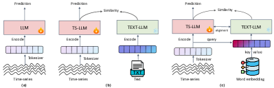
Figure 1: Comparison on LLMs for Time Series frameworks. (a) Sequential Structure (b) Parallel Structure (c) TS-TCD (ours).

The introduction of LLMs into time-series forecasting has led to two primary strategies in the literature: sequential approaches and parallel approaches. In the sequential approach, time-series data is tokenized and transformed into a format that LLMs can process, such as discrete tokens. Works such as [17, 18, 19, 20, 21, 22] employ this strategy, leveraging the strong sequence modeling capabilities of LLMs to extract complex temporal patterns. However, the challenge of modality mismatch—the inherent difference between time-series data and natural language—poses a significant barrier, often leading to performance degradation and catastrophic forgetting during fine-tuning [23, 21]. These works highlight the need for improved modality alignment, especially when adapting pre-trained LLMs to non-linguistic data like time series. In contrast, parallel approaches simultaneously encode both time-series data and textual modalities, enabling a more semantically rich representation. Prior works [24, 25, 26, 27, 28, 29] have explored multimodal learning frameworks where paired data across modalities allows for mutual knowledge transfer. While this method can enhance representation learning, it faces the limitation of requiring paired textual data, which is scarce in time-series applications. Time-series data is often collected directly by sensors or smart devices, with little or no accompanying textual information. Although some methods [30, 31] for textualizing time-series data have been proposed, they lack diversity and flexibility. Previous efforts to overcome this limitation have been constrained by their reliance on synthetic or manually generated text, which often lacks temporal coherence with the underlying time-series data.

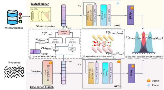
Figure 2: Overview of our method TS-TCD. During training stage, the time series branch is trained online using LoRA [32], while the language branch remains fixed. In inference stage, predictions are made solely from the time series branch.

In this paper, we address these challenges by introducing a novel triplet-level cross-modal knowledge distillation framework that merges the adaptability of sequential methods with the multi-level distillation capabilities of parallel approaches. Unlike existing methods, our framework does not rely on real paired textual data. Instead, we propose a dynamic adaptive gating mechanism to generate virtual text tokens by combining time-series data with QR-decomposed word embeddings from the LLM’s vocabulary. This novel mechanism ensures temporal coherence and alignment between modalities, overcoming the limitations of prior parallel approaches. Furturemore, we adopt layer-wise contrastive learning, and optimal transport loss to ensure consistent knowledge transfer and alignment at all stages. While contrastive learning has been used in cross-modal settings to maintain feature consistency [33, 34], its application to align intermediate layers of LLMs and time-series models remains unexplored. Moreover, the combination of contrastive loss with optimal transport for output alignment is a novel contribution in cross-modal distillation, particularly in the context of time-series forecasting. The main contributions of this paper are as follows:

• We propose a novel cross-modal knowledge distillation framework that integrates dynamic adaptive gating to align and generate virtual text.

• We introduce the combination of layer-wise contrastive learning and optimal transport loss to align intermediate representations and output distributions, a novel approach in the context of time-series forecasting.

• We demonstrate the effectiveness of the proposed framework through extensive experiments, achieving near state-of-the-art performance on both long-term and short-term forecasting tasks across benchmark time-series datasets.

II Preliminaries

In this study, we employ a dual-tower architecture to facilitate the transfer of knowledge from the textual domain ($\mathcal{D}_{text}$) to the time-series domain ($\mathcal{D}_{time}$) via a transformation function $T$:

$$T:\mathcal{D}_{text}\to\mathcal{D}_{time}$$

We define the domains as follows:

$$\mathcal{D}=\{p(\mathbf{X}),p(\mathbf{X},\mathbf{y}),p(\mathbf{y})\}$$

Introducing the intermediate layer representation $h$, In the model, we have $p(\mathbf{X},\mathbf{y})=\int p(\mathbf{y}\mid\mathbf{h})\,p(\mathbf{h}\mid\mathbf{X})\,p(\mathbf{X})\,d\mathbf{h}$ and $p(\mathbf{y})=\int\int p(\mathbf{y}\mid\mathbf{h})\,p(\mathbf{h}\mid\mathbf{X})\,p(\mathbf{X})\,d\mathbf{h}\,d\mathbf{X}$.

III Method Overview

As shown in fig. 2, we propose a dual-tower cross-modal knowledge distillation framework for time series forecasting using a language model. Both the time series student and language teacher branches share the same architecture and pre-trained weights. First, the time-series is encoded (section III-A1). Then, virtual text tokens are generated by combining the encoded time-series and the QR-decomposed language model vocabulary section III-A2 via dynamic adaptive gating (section III-A3). layer-wise contrastive learning (section III-B) and optimal transport loss (section III-C) ensure alignment between the time series and virtual text representations, with the overall loss defined in section III-D.

III-A Dynamic Adaptive Gating for Input Encoding and Alignment

In the input phase, we encode time-series data into tokens, apply QR decomposition to the word embeddings, and generate virtual text tokens using a dynamic adaptive gating mechanism.

III-A1 Time-Series Encoding

Given a multivariate time series $I\in\mathbb{R}^{L\times P}$, where $L$ is the sequence length and $P$ is the number of variables, an embedding layer maps each variable across timestamps into a shared latent space[9]. Multi-Head Self-Attention (MHSA) is then applied to obtain the time series tokens $X_{\text{time}}=\text{MHSA}(\text{Embedding}(I))\in\mathbb{R}^{P\times M}$, with $M$ as the feature dimension of the pre-trained large language models (LLMs). The resulting token set is $X_{\text{time}}=\{x_{i}^{\text{time}}\mid i=1,2,\ldots,P\}$, where $x_{i}^{\text{time}}$ are ordered tokens, and $i$ denotes their position in the sequence.

III-A2 QR-decomposed Word Embedding

In pre-trained LLMs, word embeddings serve as pivotal anchors, structuring and expanding the input distribution within the feature space. To leverage this structured distribution, the vocabulary of the language model $\hat{D}=\{v_{1}^{\text{text}},v_{2}^{\text{text}},\ldots,v_{Q}^{\text{text}}\}$ is derived by performing QR decomposition on the word embedding dictionary $D\in\mathbb{R}^{|A|\times M}$ to reduce its dimensionality. Specifically, the QR decomposition factorizes the matrix $D$ into an orthogonal matrix $Q$ and an upper triangular matrix $R$. By selecting the first $d$ vectors from $Q$ (corresponding to the rank of $R$), we construct a reduced principal embedding matrix $\hat{D}=Q_{[:,:d]}\in\mathbb{R}^{d\times M}$, where $d\ll|A|$. The orthogonality of $Q$ ensures that the selected vectors are linearly independent, unlike those obtained through PCA [31] or representative selection [22], allowing them to effectively span a subspace of the language model’s feature space.

III-A3 Virtual Text Generation via Dynamic Adaptive Gating

The text representation $X_{text}\in\mathbb{R}^{P\times M}$ is generated from $X_{time}$ by applying self-attention within the time series token and prompt-enhanced cross-attention with $\hat{D}$. The attention mechanism is described by:

$$X_{att} ={\rm Softmax}\left(\frac{QK^{T}}{\sqrt{C}}\right)V,$$ (1)

$$Q =X_{time}W_{q},$$

$$\mathbf{K}_{\text{self}},\mathbf{V}_{\text{self}} =X_{time}\mathbf{W}_{k}^{\text{self}},X_{time}\mathbf{W}_{v}^{\text{self}}\text{ (self-attention)},$$

$$\mathbf{K}_{\text{cross}},\mathbf{V}_{\text{cross}} =[\mathbf{P}_{k};\hat{\mathbf{D}}\mathbf{W}_{k}^{\text{cross}}],[\mathbf{P}_{v};\hat{\mathbf{D}}\mathbf{W}_{v}^{\text{cross}}]\text{(Cross-Attention)},$$

The primary difference between self-attention and cross-attention lies in the source of the keys ($\mathbf{K}$) and values ($\mathbf{V}$), resulting in $\mathbf{X}_{\text{self}}$ and $\mathbf{X}_{\text{cross}}$ being obtained. $P_{k}\in\mathbb{R}^{L_{p}\times d_{k}}$ and $P_{v}\in\mathbb{R}^{L_{p}\times d_{k}}$ are the learnable prompt matrices with $L_{p}$ being the prompt length and $d_{k}$ being the dimensionality of each attention head. The prompts guide the cross-attention process, aligning time series data with text representations by focusing on task-relevant features[35], and compensating for the possible absence of key-value pairs, ensuring effective handling of unseen time-series tokens. The final text representation $X_{text}$ is obtained by adaptively combining the outputs from self-attention and cross-attention:

$$g=\text{Sigmoid}\left(W_{\text{gate}}^{T}[X_{cross};X_{self}]\right)$$ (2)

$$X_{text}=X_{cross}\odot g+X_{self}\odot(1-g),$$

Here $W_{\text{gate}}^{T}\in\mathbb{R}^{2d_{k}\times d_{k}}$ and $g\in\mathbb{R}^{d_{k}\times d_{k}}$. This dual attention effectively integrates the time series and language information, enabling the generation of virtual text data based on time-series features, thereby facilitating cross-modal learning and downstream applications.

III-B Layer-Wise Contrastive Learning for Intermediate Network Alignment

To align the outputs of each intermediate layer in the temporal student branch with those in the textual teacher branch, we use a layer-wise contrastive learning method. This approach enhances the alignment of semantically congruent information between modalities by optimizing relative similarity in the feature space, rather than minimizing absolute differences[31]. Specifically, we apply the InfoNCE loss at each layer:

$$L_{\text{InfoNCE}}^{m}=-\frac{1}{N}\sum_{i=1}^{N}\log\frac{\exp\left(\text{sim}\left(F_{\text{time}}^{i},F_{\text{text}}^{i}\right)/\tau\right)}{\sum_{j=1}^{K}\exp\left(\text{sim}\left(F_{\text{time}}^{i},F_{\text{text}}^{j}\right)/\tau\right)},$$ (3)

where $\text{sim}(\cdot,\cdot)$ denotes the similarity function, and $\tau$ is the temperature parameter. The terms $F_{\text{time}}^{i}(\cdot)$ and $F_{\text{text}}^{i}(\cdot)$ represent the aggregated intermediate features from the temporal and textual modalities, respectively, where average pooling has been applied to combine all tokens within each layer. The overall feature loss $\mathcal{L}_{\text{feature}}$ integrates these losses across layers:

$$\mathcal{L}_{\text{feature}}=\sum_{m=1}^{L}\gamma^{(L-m)}L_{\text{InfoNCE}}^{m},$$ (4)

where a decay factor $\gamma^{(L-m)}$ is applied to give more weight to losses from layers closer to the input, reflecting their importance in the alignment process. This ensures that corresponding time-series and language token representations are closely aligned, while non-corresponding tokens are pushed apart.

III-C Optimal Transport-Driven Alignment in the Output Layer

To achieve coherent and unified predictions from both the time-series and language modalities, we adpot optimal transport (OT) [36] to ensure distribution consistency in the output layer. Unlike the traditional $L_{2}$ loss, which captures pointwise differences, OT aligns these distributions holistically, making it more effective at capturing semantic relationships between the two modalities. The loss function is defined as:

$$\mathcal{L}_{\text{ot}}=\sum_{i,j}P_{ij}\,W_{ij}+\mu H(P_{ij})$$ (5)

Where $P_{ij}$ represents the optimal transport plan, and $W_{ij}=W(Y_{\text{time}},Y_{\text{text}})$ is the cost matrix based on the pairwise distances between $Y_{\text{time}}$ and $Y_{\text{text}}$. The entropy term $H(P_{ij})$ regularizes the transport plan, with $\mu$ controlling the trade-off between minimizing transport cost and encouraging smoother solutions. The Sinkhorn algorithm [37] is employed to solve this problem. By using this $\mathcal{L}_{\text{ot}}$ loss, we ensure that the different modalities converge, maintaining a consistent semantic space for high-level tasks in multimodal learning.

III-D Total Loss Function for Cross-Modal Distillation

To ensure effective training and alignment of the model across modalities, we employ a combined loss function that integrates various components. Specifically, the total loss for the textural student branch, following [38, 31], is a weighted sum of the supervised loss of task $\mathcal{L}_{\text{task}}$, the feature alignment loss $\mathcal{L}_{\text{feature}}$, and the output consistency loss $\mathcal{L}_{\text{ot}}$. The total loss $\mathcal{L}_{\text{total}}$ is given by:

$$\mathcal{L}_{\text{total}}=\mathcal{L}_{\text{task}}+\alpha\mathcal{L}_{\text{feature}}+\beta\mathcal{L}_{\text{ot}}$$ (6)

where $\alpha$ and $\beta$ are hyperparameters that balance the contributions.

TABLE I: Multivariate long-term forecasting results with input length $T=96$. Results are averaged over 4 prediction lengths $H\in\{96,192,336,720\}$. A lower value indicates better performance, and this applies to all subsequent tables.

Models	Ours		CALF[31]		TimeLLM[20]		GPT4TS[23]		PatchTST[8]		iTransformer[9]		Crossformer[10]		FEDformer[12]		TimesNet		MICN[6]		DLinear[14]		TiDE[15]
Metric	MSE	MAE	MSE	MAE	MSE	MAE	MSE	MAE	MSE	MAE	MSE	MAE	MSE	MAE	MSE	MAE	MSE	MAE	MSE	MAE	MSE	MAE	MSE	MAE
ETTm1	0.383	0.373	0.395	0.390	0.410	0.409	0.389	0.397	0.381	0.395	0.407	0.411	0.502	0.502	0.448	0.452	0.400	0.406	0.392	0.413	0.403	0.407	0.412	0.406
ETTm2	0.276	0.301	0.281	0.321	0.296	0.340	0.285	0.331	0.285	0.327	0.291	0.335	1.216	0.707	0.305	0.349	0.291	0.333	0.328	0.382	0.350	0.401	0.289	0.326
ETTh1	0.423	0.405	0.432	0.428	0.460	0.449	0.447	0.436	0.450	0.441	0.455	0.448	0.620	0.572	0.440	0.460	0.458	0.450	0.558	0.535	0.456	0.452	0.445	0.432
ETTh2	0.351	0.361	0.349	0.382	0.389	0.408	0.381	0.408	0.366	0.394	0.381	0.405	0.942	0.684	0.437	0.449	0.414	0.427	0.587	0.525	0.559	0.515	0.611	0.550
Weather	0.248	0.260	0.250	0.274	0.274	0.290	0.264	0.284	0.258	0.280	0.257	0.279	0.259	0.315	0.309	0.360	0.259	0.287	0.242	0.299	0.265	0.317	0.271	0.320
Electricity	0.164	0.254	0.175	0.265	0.223	0.309	0.205	0.290	0.216	0.304	0.178	0.270	0.244	0.334	0.214	0.327	0.192	0.295	0.186	0.294	0.212	0.300	0.251	0.344
Traffic	0.425	0.285	0.439	0.281	0.541	0.358	0.488	0.317	0.555	0.361	0.428	0.282	0.550	0.304	0.610	0.376	0.620	0.336	0.541	0.315	0.625	0.383	0.760	0.473
1st Place	10		2		0		0		1		0		0		0		0		1		0		0

IV Experiments

TABLE II: Short-term forecasting results on the M4 dataset. Input lengths are $[12,96]$ and corresponding predictions are $[6,48]$. The results are weighted averages across datasets under different sampling intervals.

Models		Ours	CALF[31]	TimeLLM[20]	GPT4TS[23]	PatchTST[8]	ETSformer[11]	FEDformer[12]	Autoformer[13]	TimesNet[7]	TCN[5]	N-HiTS[39]	N-BEATS[40]	DLinear[14]
Average	SMAPE	11.651	11.765	11.983	11.991	12.059	14.718	12.840	12.909	11.829	13.961	11.927	11.851	13.639
	MASE	1.563	1.567	1.595	1.600	1.623	2.408	1.701	1.771	1.585	1.945	1.613	1.599	2.095
	OWA	0.837	0.844	0.859	0.861	0.869	1.172	0.918	0.939	0.851	1.023	0.861	0.855	1.051
1st Place		3	0	0	0	0	0	0	0	0	0	0	0	0

We evaluated our framework on standard time-series forecasting benchmarks, comparing it with state-of-the-art models for both long-term table I and short-term forecasting table II, in line with competitive research [31, 20, 7]. Ablation studies (table III) were conducted to assess the impact of individual components. All experiments were conducted under uniform settings across models, adhering to established protocols [7], with evaluation pipelines available online.

IV-A Implementation Details.

Following [23], we used GPT-2 [41] with its first six Transformer layers as the backbone. The Adam optimizer [42] was applied with a learning rate of $5\times 10^{-4}$. Loss hyperparameters were set to $\alpha=0.1$, and $\beta=0.01$. Task loss is smooth $L1$ for long-term forecasting, and smape for shot-term forecasting. The Optimal Transport parameter is set to $\mu=0.1$, and the number of iterations is set to 100. InfoNCE is implemented based on the Lightly toolbox. The decay factor is set to $\gamma=0.8$ to balance the lower and higher layers.

IV-B Experiment Results

Overall Performance. 1) Long-term Forecasting: TS-TCD outperforms baseline models like TimeLLM[20] and CALF[31], as shown in table I. On the ETTm2 dataset, it achieves an MAE of 0.301, a 6.2% improvement over CALF (0.321). For Electricity, TS-TCD achieves an MSE of 0.164, 6.3% lower than CALF’s 0.175. It also demonstrates superior performance on Weather and Electricity datasets, effectively capturing long-term dependencies.

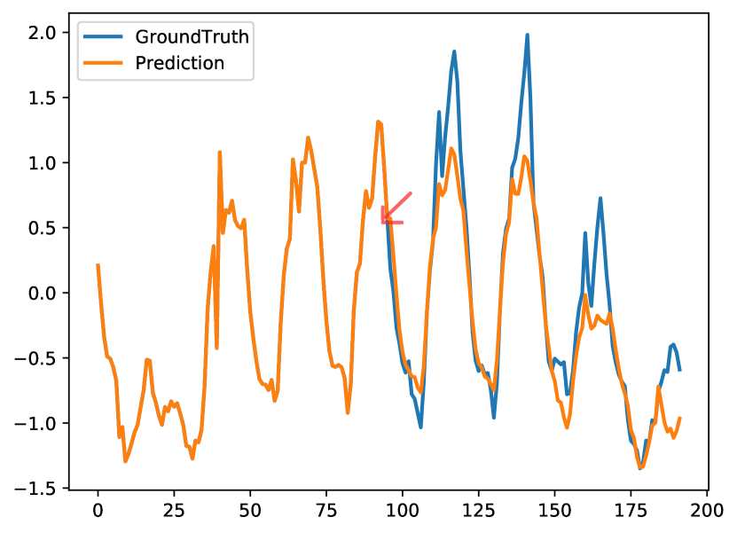
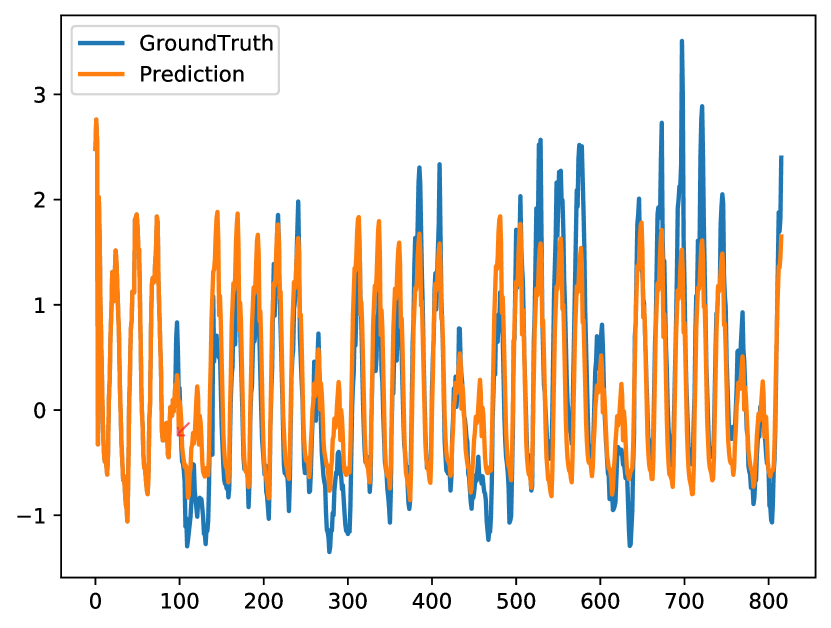
Figure 3: Long-term forecasting visualization cases for Electricity. The blue lines represent the actual values, while the orange lines indicate the model’s predictions.

2) Short-term Forecasting: In short-term tasks, TS-TCD leads with the lowest SMAPE (11.651), MASE (1.563), and OWA (0.837) across average intervals table II, improving on CALF by 3.5%. Overall, LLM-based methods[31, 20, 23] outperform traditional MLP-based[14, 15], CNN[5, 6, 7], and Transformer models[8, 9, 10, 11, 12, 13], due to their enhanced ability to capture contextual information and generalize across diverse tasks. TS-TCD demonstrates higher accuracy and resilience across both long- and short-term forecasting, making it a versatile solution for time-series data.

Ablation Studies. We performed ablation studies to assess the impact of each component: Dynamic Adaptive Gating (DAG), feature loss ($\mathcal{L}{feature}$), and optimal transport loss ($\mathcal{L}{ot}$). Table III shows that removing DAG increases SMAPE by 3.4% (+0.394), proving its importance. The full model achieves the best SMAPE (11.651), confirming the necessity of all components. Alignment modules roughly have the greatest impact at the input stage and the least at the output stage.

Visualization. fig. 3 shows long-term forecasting results for the Electricity dataset. On the left, the prediction is for 96 time steps, while on the right, it extends to 720 time steps. In both cases, our model consistently performs well, closely aligning its predictions with the ground truth.

TABLE III: Ablation study on the M4 dataset using average interval metrics. DAG represents dynamic adaptive gating.

Model	DAG	$\mathcal{L}_{feature}$	$\mathcal{L}_{ot}$	M4
				SMAPE	MASE	OWA
1	✓	$-$	$-$	11.821	1.678	0.892
2	$-$	✓	$-$	11.844	1.567	0.864
3	$-$	$-$	✓	11.956	1.621	0.881
Ours	✓	✓	✓	11.651	1.563	0.837

V Conclusion

In this paper, we proposed TS-TCD, a novel framework designed to enhance time-series forecasting by integrating LLMs through a triplet-level cross-modal distillation process. Unlike existing methods that focus on individual alignment components, TS-TCD provides a holistic approach by aligning input, feature, and output layers across modalities. Our dynamic adaptive gating mechanism addresses input modality mismatch by generating virtual text tokens that are coherently aligned with time-series data. Additionally, layer-wise contrastive learning ensures intermediate feature consistency, while optimal transport-driven output alignment reduces discrepancies at the task level. Experimental results highlight the framework’s superior performance across multiple benchmarks, confirming the value of integrating these mechanisms.

References

- [1] A. Muhammed, K. S. Olaosun, S. J. Popoola, and J. Byers, “Deep learning in finance: Time series prediction,” 2024.
- [2] P. Gao, T. Liu, J.-W. Liu, B.-L. Lu, and W.-L. Zheng, “Multimodal multi-view spectral-spatial-temporal masked autoencoder for self-supervised emotion recognition,” in ICASSP 2024 - 2024 IEEE International Conference on Acoustics, Speech and Signal Processing (ICASSP), 2024, pp. 1926–1930.
- [3] P. Liu, B. Wu, N. Li, T. Dai, F. Lei, J. Bao, Y. Jiang, and S.-T. Xia, “Wftnet: Exploiting global and local periodicity in long-term time series forecasting,” in ICASSP 2024-2024 IEEE International Conference on Acoustics, Speech and Signal Processing (ICASSP). IEEE, 2024, pp. 5960–5964.
- [4] J. Pan, W. Ji, B. Zhong, P. Wang, X. Wang, and J. Chen, “Duma: Dual mask for multivariate time series anomaly detection,” IEEE Sensors Journal, vol. 23, no. 3, pp. 2433–2442, 2022.
- [5] S. Bai, J. Z. Kolter, and V. Koltun, “An empirical evaluation of generic convolutional and recurrent networks for sequence modeling,” arXiv preprint arXiv:1803.01271, 2018.
- [6] H. Wang, J. Peng, F. Huang, J. Wang, J. Chen, and Y. Xiao, “MICN: Multi-scale local and global context modeling for long-term series forecasting,” in International Conference on Learning Representations, 2022.
- [7] H. Wu, T. Hu, Y. Liu, H. Zhou, J. Wang, and M. Long, “Timesnet: Temporal 2d-variation modeling for general time series analysis,” ArXiv, vol. abs/2210.02186, 2022.
- [8] Y. Nie, N. H. Nguyen, P. Sinthong, and J. Kalagnanam, “A time series is worth 64 words: Long-term forecasting with transformers,” in International Conference on Learning Representations, 2023.
- [9] Y. Liu, T. Hu, H. Zhang, H. Wu, S. Wang, L. Ma, and M. Long, “itransformer: Inverted transformers are effective for time series forecasting,” arXiv preprint arXiv:2310.06625, 2023.
- [10] Y. Zhang and J. Yan, “Crossformer: Transformer utilizing cross-dimension dependency for multivariate time series forecasting,” in International Conference on Learning Representations, 2023.
- [11] G. Woo, C. Liu, D. Sahoo, A. Kumar, and S. C. H. Hoi, “ETSformer: Exponential smoothing transformers for time-series forecasting,” arXiv preprint arXiv:2202.01381, 2022.
- [12] T. Zhou, Z. Ma, Q. Wen, X. Wang, L. Sun, and R. Jin, “FEDformer: Frequency enhanced decomposed transformer for long-term series forecasting,” in International Conference on Machine Learning. PMLR, 2022, pp. 27 268–27 286.
- [13] H. Wu, J. Xu, J. Wang, and M. Long, “Autoformer: Decomposition transformers with Auto-Correlation for long-term series forecasting,” in Advances in Neural Information Processing Systems, 2021.
- [14] A. Zeng, M. Chen, L. Zhang, and Q. Xu, “Are transformers effective for time series forecasting?” in Proceedings of the AAAI conference on artificial intelligence, vol. 37, 2023, pp. 11 121–11 128.
- [15] A. Das, W. Kong, A. Leach, R. Sen, and R. Yu, “Long-term forecasting with TiDE: Time-series dense encoder,” arXiv preprint arXiv:2304.08424, 2023.
- [16] Y. Liang, H. Wen, Y. Nie, Y. Jiang, M. Jin, D. Song, S. Pan, and Q. Wen, “Foundation models for time series analysis: A tutorial and survey,” in Proceedings of the 30th ACM SIGKDD Conference on Knowledge Discovery and Data Mining, 2024, pp. 6555–6565.
- [17] H. Xue and F. D. Salim, “Promptcast: A new prompt-based learning paradigm for time series forecasting,” IEEE Transactions on Knowledge and Data Engineering, 2023.
- [18] D. Cao, F. Jia, S. O. Arik, T. Pfister, Y. Zheng, W. Ye, and Y. Liu, “Tempo: Prompt-based generative pre-trained transformer for time series forecasting,” arXiv preprint arXiv:2310.04948, 2023.
- [19] C. Chang, W.-C. Peng, and T.-F. Chen, “Llm4ts: Two-stage fine-tuning for time-series forecasting with pre-trained llms,” arXiv preprint arXiv:2308.08469, 2023.
- [20] M. Jin, S. Wang, L. Ma, Z. Chu, J. Y. Zhang, X. Shi, P.-Y. Chen, Y. Liang, Y.-F. Li, S. Pan et al., “Time-llm: Time series forecasting by reprogramming large language models,” arXiv preprint arXiv:2310.01728, 2023.
- [21] Z. Pan, Y. Jiang, S. Garg, A. Schneider, Y. Nevmyvaka, and D. Song, “ip-llm: Semantic space informed prompt learning with llm for time series forecasting,” arXiv preprint arXiv:2403.05798, 2024.
- [22] C. Sun, Y. Li, H. Li, and S. Hong, “Test: Text prototype aligned embedding to activate llm’s ability for time series,” arXiv preprint arXiv:2308.08241, 2023.
- [23] T. Zhou, P. Niu, X. Wang, L. Sun, and R. Jin, “One fits all: Power general time series analysis by pretrained lm,” arXiv preprint arXiv:2302.11939, 2023.
- [24] Z. Wang and H. Ji, “Open vocabulary electroencephalography-to-text decoding and zero-shot sentiment classification,” in Proceedings of the AAAI Conference on Artificial Intelligence, vol. 36, no. 5, 2022, pp. 5350–5358.
- [25] J. Qiu, W. Han, J. Zhu, M. Xu, D. Weber, B. Li, and D. Zhao, “Can brain signals reveal inner alignment with human languages?” in Findings of the Association for Computational Linguistics: EMNLP 2023, 2023, pp. 1789–1804.
- [26] J. Li, C. Liu, S. Cheng, R. Arcucci, and S. Hong, “Frozen language model helps ecg zero-shot learning,” in Medical Imaging with Deep Learning. PMLR, 2024, pp. 402–415.
- [27] F. Jia, K. Wang, Y. Zheng, D. Cao, and Y. Liu, “Gpt4mts: Prompt-based large language model for multimodal time-series forecasting,” in Proceedings of the AAAI Conference on Artificial Intelligence, vol. 38, no. 21, 2024, pp. 23 343–23 351.
- [28] H. Yu, P. Guo, and A. Sano, “Ecg semantic integrator (esi): A foundation ecg model pretrained with llm-enhanced cardiological text,” arXiv preprint arXiv:2405.19366, 2024.
- [29] J. W. Kim, A. Alaa, and D. Bernardo, “Eeg-gpt: Exploring capabilities of large language models for eeg classification and interpretation,” arXiv preprint arXiv:2401.18006, 2024.
- [30] Y. Wang, R. Jin, M. Wu, X. Li, L. Xie, and Z. Chen, “K-link: Knowledge-link graph from llms for enhanced representation learning in multivariate time-series data,” arXiv preprint arXiv:2403.03645, 2024.
- [31] P. Liu, H. Guo, T. Dai, N. Li, J. Bao, X. Ren, Y. Jiang, and S.-T. Xia, “Taming pre-trained llms for generalised time series forecasting via cross-modal knowledge distillation,” arXiv preprint arXiv:2403.07300, 2024.
- [32] E. J. Hu, Y. Shen, P. Wallis, Z. Allen-Zhu, Y. Li, S. Wang, L. Wang, and W. Chen, “Lora: Low-rank adaptation of large language models,” arXiv preprint arXiv:2106.09685, 2021.
- [33] Z. Wang and C. Ma, “Dual-contrastive dual-consistency dual-transformer: A semi-supervised approach to medical image segmentation,” in Proceedings of the IEEE/CVF International Conference on Computer Vision, 2023, pp. 870–879.
- [34] J. Wu, W. Sun, T. Gan, N. Ding, F. Jiang, J. Shen, and L. Nie, “Neighbor-guided consistent and contrastive learning for semi-supervised action recognition,” IEEE Transactions on Image Processing, vol. 32, pp. 2215–2227, 2023.
- [35] Y.-L. Lee, Y.-H. Tsai, W.-C. Chiu, and C.-Y. Lee, “Multimodal prompting with missing modalities for visual recognition,” in Proceedings of the IEEE/CVF Conference on Computer Vision and Pattern Recognition, 2023, pp. 14 943–14 952.
- [36] C. Villani, Topics in optimal transportation. American Mathematical Soc., 2021, vol. 58.
- [37] M. Cuturi, “Sinkhorn distances: Lightspeed computation of optimal transport,” Neural Information Processing Systems,Neural Information Processing Systems, Dec 2013.
- [38] Y. Liu, G. Qin, X. Huang, J. Wang, and M. Long, “Autotimes: Autoregressive time series forecasters via large language models,” arXiv preprint arXiv:2402.02370, 2024.
- [39] C. Challu, K. G. Olivares, B. N. Oreshkin, F. Garza, M. Mergenthaler, and A. Dubrawski, “N-HiTs: Neural hierarchical interpolation for time series forecasting,” arXiv preprint arXiv:2201.12886, 2022.
- [40] B. N. Oreshkin, D. Carpov, N. Chapados, and Y. Bengio, “N-BEATS: Neural basis expansion analysis for interpretable time series forecasting,” International Conference on Learning Representations, 2019.
- [41] A. Radford, J. Wu, R. Child, D. Luan, D. Amodei, I. Sutskever et al., “Language models are unsupervised multitask learners,” 2019.
- [42] D. P. Kingma and J. Ba, “Adam: A method for stochastic optimization,” arXiv preprint arXiv:1412.6980, 2014.