Evaluating Machine Learning Models for Supernova Gravitational Wave Signal Classification

Abstract

We investigate the potential of using gravitational wave (GW) signals from rotating core-collapse supernovae to probe the equation of state (EOS) of nuclear matter. By generating GW signals from simulations with various EOSs, we train machine learning models to classify them and evaluate their performance. Our study builds on previous work by examining how different machine learning models, parameters, and data preprocessing techniques impact classification accuracy. We test convolutional and recurrent neural networks, as well as six classical algorithms: random forest, support vector machines, naïve Bayes, logistic regression, $k$-nearest neighbors, and eXtreme gradient boosting. All models, except naïve Bayes, achieve over 90 per cent accuracy on our dataset. Additionally, we assess the impact of approximating the GW signal using the general relativistic effective potential (GREP) on EOS classification. We find that models trained on GREP data exhibit low classification accuracy. However, normalizing time by the peak signal frequency, which partially compensates for the absence of the time dilation effect in GREP, leads to a notable improvement in accuracy.

I Introduction

Gravitational waves (GWs) are ripples in the fabric of space-time that travel at the speed of light. GWs can traverse the cosmos without significant disturbance, reaching Earth mostly unchanged and providing a clear view of their sources. To date, GW detections have come from black hole mergers [1], neutron star mergers [2], and black hole-neutron star mergers [3], offering unprecedented insights into these phenomena. Another promising source of GWs is core-collapse supernovae (CCSNe), which could greatly enhance our understanding of these events [4, 5, 6, 7, 8, 9]. Current GW observatories can detect supernova signals from within our Galaxy, expected once or twice per century [10, 11]. Future detectors will have higher sensitivity, enabling them to observe more distant events [12].

CCSNe are powerful explosions that mark the death of massive stars. As these stars age, they undergo successive stages of nuclear fusion, ultimately forming a dense core of iron-group nuclei. Once the core reaches large enough mass, the electron degeneracy pressure can no longer support it against gravity, causing it to collapse. The collapse is abruptly halted upon reaching nuclear densities, triggering a rebound that generates a shock wave. For a supernova explosion to occur, the shock must expel the star’s outer layers, leaving behind a stable neutron star. Otherwise, a black hole forms [13, 14, 15]. The precise mechanisms behind this process is a focus of ongoing research [16, 17, 18, 19, for recent reviews].

Neutrinos play a key role in CCSNe. The protoneutron star (PNS) cools by emitting vast numbers of neutrinos [20, 21]. A small fraction of them are absorbed behind the shock, depositing their energy and heating the region [22, 23]. This heating induces convection [24, 25, 26], which, along with the potential development of standing accretion shock instability (SASI) [27, 28], helps push the shock front outward, driving the explosion.

In rare cases, stars are rapidly rotating and the PNSs are born with substantial rotational kinetic energy [29, 30, 31, 32, 33]. Magnetic fields can transfer this energy to the shock, potentially causing more powerful hypernova explosions [34] and possibly triggering long gamma-ray bursts [35, 36].

The supernova GWs are predominantly emitted by the PNS dynamics [37, 38, for recent reviews]. Neutrino-driven convection and SASI perturb the flow, driving PNS oscillations [39, 40, 41, 42, 43]. In rapidly rotating stars, the centrifugal force causes the collapse to become deformed, resulting in a core bounce with quadrupolar deformation. This excites oscillations of the PNS that last for $\sim 10$ ms after bounce [44]. This type of signal is usually called the rotating bounce GW signal.

Gravitational waves originating from the PNS oscillations carry valuable information about its structure [45, 46, 40, 47, 48, 49]. In particular, the signal depends on the poorly understood properties of high-density nuclear matter [50, 6, 51, 52]. This offers an opportunity to constrain the parameters of the nuclear equation of state (EOS) using GW data [53, 54].

Recently, machine learning (ML) has shown significant promise in inferring source parameters from GW signals [53, 55, 56, 57, 58, 59, 60, 61, 62, 63, 64]. It has proven particularly effective for rotating bounce signals, which are easier to model and cost-efficient to simulate, allowing the generation of large GW datasets necessary for ML training [65]. In [53, 54], convolutional neural networks were applied to EOS classification using the GW database from [50]. Mitra et al. [65] extended this work by incorporating uncertainties in electron capture rates during collapse, which influence the dynamics and, consequently, the GW signal.

In this work, we expand on previous studies in two key ways. First, we investigate how classification accuracy is affected by different ML model types, parameters, and data preprocessing techniques. Second, we examine the impact of a GW signal approximation based on the general relativistic effective potential (GREP) [66, 67, 68], which modifies the gravitational potential to approximate general relativistic (GR) effects within a Newtonian framework. The main advantage of this method is its simplicity and lower computational cost compared to full GR simulations. However, the main drawback is that while GREP can mimic GR gravity, it does not capture other relativistic effects, such as time dilation or length contraction. We assess how well ML models trained on the GW signals generated using the GREP approximation can classify the EOS from the rotational bounce GW signal.

This paper organized as following. In Section II, we describe our dataset, ML methods, and accuracy evaluation criteria. In Section III, we present our results. Finally, in Section IV, we summarize our results and provide conclusions.

II Methodology

In this section, we describe the dataset, the ML algorithms, hyperparameter selection, training process, and the evaluation method for EOS classification.

II.1 Data

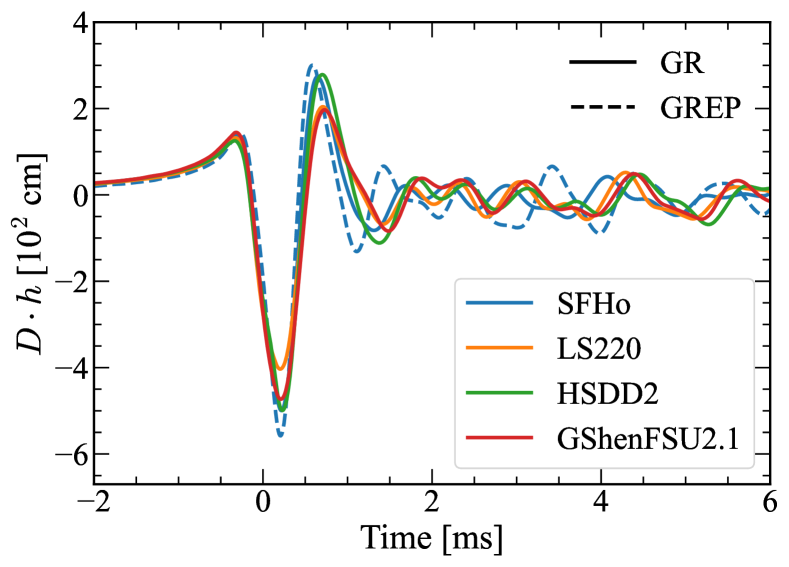
Figure 1: Gravitational wave strain as a function of time for models with $T/|W|\approx 0.09$. The blue, yellow, green, and red curves represent SHFo, LS220, HSDD2, and GShenFSU2.1 EOSs, respectively. Solid and dashed lines correspond to GR and GREP waveforms, respectively. The zero time corresponds to the time of bounce.

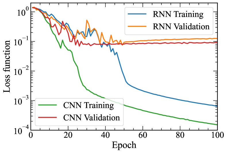
Figure 2: The training and validation losses as a function of epochs are shown as blue and orange curves for the RNN, and green and red curves for the CNN. In this particular train-test split case, the minimal validation loss occurs at epoch 26 for the CNN and at epoch 49 for the RNN. After these points, the validation loss stops improving while the training loss continues to decrease, indicating overfitting.

Table 1: Architecture of the CNN model used in the study. The model consists of ten layers, starting with an Input layer, followed by three Convolutional layers, each paired with Max Pooling layers, and ending with three Dense layers after a Flatten layer. The table provides information on the type of each layer, the number of filters or units, the kernel size, the pooling size, the output shape at each layer, and the corresponding activation functions. The final Dense layer with 4 units and a Softmax activation function is used for classification.

Layer	Type	Parameters	Output Shape	Activation
0	Input		(81)
1	Convolution 1D	32 filters, kernel size 3	(79, 32)	ReLU
2	Max Pooling 1D	Pool size 2	(39, 32)
3	Convolution 1D	64 filters, kernel size 3	(37, 64)	ReLU
4	Max Pooling 1D	Pool size 2	(18, 64)
5	Convolution 1D	128 filters, kernel size 3	(16, 128)	ReLU
6	Max Pooling 1D	Pool size 2	(8, 128)
7	Flatten		(1024)
7	Dense	512 units	(512)	ReLU
8	Dense	256 units	(256)	ReLU
9	Dense	4 units	(4)	Softmax

Table 2: Architecture of the RNN model employed in this study. The model consists of four layers: two SimpleRNN layers followed by two Dense layers. The SimpleRNN layers contain 64 and 128 units, respectively, while the Dense layers include 64 units with ReLU activation and 4 units with Softmax activation, facilitating the final classification output.

Layer	Type	Parameters	Output Shape	Activation
0	SimpleRNN	64 units	(81, 64)
1	SimpleRNN	128 units	(128)
2	Dense	64 units	(64)	ReLU
3	Dense	4 units	(4)	Softmax

Table 3: Grid of hyperparameters used for tuning classical machine learning models. The optimal hyperparameters are highlighted in bold.

Random Forest	Support Vector Machines	Naïve Bayes
’n_estimators’: [50, 75, 100, 125, 150] ’max_depth’: [None, 10, 15, 20] ’min_samples_split’: [2, 5, 10] ’min_samples_leaf’: [1, 2, 4]	’C’: [0.1, 1, 10] ’kernel’: [’linear’, ’rbf’, ’poly’] ’gamma’: [’scale’, ’auto’] ’degree’: [2, 3, 4]	’var_smoothing’: [$10^{-9}$, $10^{-8}$, $10^{-7}$,                               $10^{-6}$, $10^{-5}$]
Logistic Regression	$k$-Nearest Neighbors	eXtreme Gradient Boosting
’C’: [0.01, 0.1, 1, 10, 100] ’penalty’: [’l1’, ’l2’, ’none’] ’solver’: [’lbfgs’, ’liblinear’, ’saga’] ’max_iter’: [100, 200, 300]	’n_neighbors’: [3, 5, 7, 9, 11] ’weights’: [’uniform’, ’distance’] ’metric’: [’euclidean’,                   ’manhattan’,                   ’minkowski’] ’p’: [1, 2]	’n_estimators’: [50, 100, 200] ’max_depth’: [3, 5, 7] ’learning_rate’: [0.01, 0.1, 0.2] ’subsample’: [0.8, 0.9, 1.0] ’colsample_bytree’: [0.8, 0.9, 1.0] ’gamma’: [0, 0.1, 0.2] ’reg_alpha’: [0, 0.01, 0.1] ’reg_lambda’: [1, 0.1, 0.01]

We obtain GWs from numerical simulations using the code CoCoNuT [69, 70]. We perform two sets of simulations. In the first set, we use GR with the conformal-flatness condition (CFC) [71, 72, 73], which yields excellent accuracy in the context of CCSNe [e.g., 74, 75, 76]. In the second set, we use Newtonian hydrodynamics with GR effective potential. We use the so-called “case A” formulation, which was found to better reproduce GR results [67] (see Appendix A for details).

The rest of the parameters are the same in both sets of simulations. We impose axisymmetry as the stellar core remains largely axisymmetric up to $\sim\!10\,\mathrm{ms}$ after bounce [76]. Magnetic fields are neglected since they do not influence the dynamics within this timescale [e.g., 31]. We use 250 logarithmical radial cells spanning $3,000$ km and 40 uniform angular cells covering the upper half of the meridional plane, assuming equatorial reflection symmetry. To model neutrino processes during collapse, we use the $Y_{e}(\rho)$ deleptonization scheme [77]. The $Y_{e}(\rho)$ profiles are obtained from 1D radiation-hydrodynamics calculations using GR1D [78]. We perform simulations for four different equations of state (EOS): SFHo [79], LS220 [80], GShenFSU2.1 [81], and HSDD2 [82, 83]. Among the 18 EOSs in the database of [50], these four EOSs best match observational and experimental constraints.

For every EOS, we consider about 100 rotational configurations of the s12 model [84], ranging from slow to rapid rotation [85]. We quantify the rotation at bounce using the parameter $T/|W|$, where $T$ is the rotational kinetic energy and $W$ is the potential binding energy. We focus on a rotation range of $0.02<T/|W|<0.18$. For $T/|W|<0.02$, the rotation is too slow to cause significant quadrupole deformations, resulting in a weak bounce signal. Conversely, for $T/|W|>0.18$, the centrifugal force becomes dominant, inhibiting the core from reaching the high densities where differences in EOS are most pronounced. In total, we have 452 GR waveforms, with 116, 120, 108, and 108 for SFHo, LS220, HSDD2, and GShenFSU2.1, respectively. For GREP, we have 412 waveforms, with 105, 105, 103, and 99 for SFHo, LS220, HSDD2, and GShenFSU2.1, respectively. As an example, Fig. 1 shows GWs for these EOSs in GR and for SFHo EOS in GREP for models with $T/|W|\simeq 0.09$.

The waveforms are sampled at a rate of 10 kHz, as the signal around or above this frequency does not have any significant physical component [e.g., 50]. Moreover, at high frequencies, quantum noise becomes the dominant factor for terrestrial detectors, making it challenging to observe signals above the noise threshold [86]. We concentrate on the time interval from $-2$ ms to $6$ ms, with zero time corresponding to the bounce. This range is selected because the GW signal before $-2$ ms contains little energy, and the signal after $6$ ms includes contributions from prompt convection, which is not accurately captured in our model [65].

II.2 Algorithms

We use two deep learning algorithms, Convolutional Neural Networks (CNN) and Recurrent Neural Networks (RNN), and six classical ML algorithms: Random Forest (RF), Support Vector Machines (SVM), Naïve Bayes (NB), Logistic Regression (LR), $k$-Nearest Neighbors ($k$-NN), and eXtreme Gradient Boosting (XGB). Before the ML analysis, all waveforms are normalized by dividing them by their amplitudes $D\cdot\Delta h$. We train our models and optimize their hyperparameters using the GR data.

CNN and RNN: We use the architecture shown in Table 1 for the CNN and Table 2 for the RNN. The dataset is split into training, validation, and test sets with a 64:16:20 ratio, maintaining the class distribution across all sets. For training, we employ the sparse categorical cross-entropy loss function, commonly used in multiclass classification, along with the Adam optimizer. Fig. 2 illustrates the loss function across epochs for both the CNN and RNN models.

During training, we apply the early stopping strategy to prevent overtraining. If the validation loss does not improve for 20 consecutive epochs in the case of the CNN, or for 40 consecutive epochs in the case of the RNN, we stop training and retain the model that achieved the minimum validation loss. We set a maximum of 100 epochs for the CNN and 200 epochs for the RNN.

Classical ML algorithms: We split our dataset with an 80:20 ratio, using the larger portion for hyperparameter tuning through the Grid Search Cross-Validation (GridSearchCV) technique [87]. GridSearchCV is a powerful tool in ML that optimizes model performance by systematically exploring a predefined hyperparameter space. It assesses the model’s performance across various parameter combinations using 5-fold cross-validation to identify the optimal settings.

In this approach, the dataset is divided into five folds. For each combination of hyperparameters, the model is trained on four of these folds and validated on the remaining fold. This process is repeated five times, with each fold serving as the validation set exactly once. The cross-validation scores, which represent EOS classification accuracy, from these iterations are averaged to evaluate the effectiveness of each parameter combination. The combination yielding the highest average performance is selected as the optimal set of hyperparameters.

To ensure that the model is neither overfitting nor underfitting, we compare the average accuracy on the validation set with the accuracy on the smaller portion of the dataset set aside initially as the test set. If the test set performance closely matches the validation set performance, it indicates that the model generalizes well. A significant drop in test accuracy would suggest potential overfitting, prompting further adjustments.

Table 3 displays the hyperparameter space for the machine learning algorithms. The optimal hyperparameters are highlighted in bold. These optimal parameters were tested on the test set and were consistent with the validation set results. We use this optimal set of hyperparameters in our analysis.

After determining the optimal set of hyperparameters, we split the dataset into training, validation, and test sets with a 64:16:20 ratio. Note that, for classical ML algorithms, the validation set is not utilized. We use 64% of the data for training and 20% for testing. This approach aligns with the data allocation used for CNN and RNN models, allowing for a fair comparison of performance across all algorithms.

To evaluate the performance of the EOS classification, we use accuracy, recall, and precision metrics. Our evaluation process involves repeating the calculations 100 times, with each iteration involving a random train-test split. We compute the average performance across all iterations and use the standard deviation as a measure of error. This methodology helps us obtain results that are independent of specific train-test split realizations, thereby demonstrating the robustness of our findings.

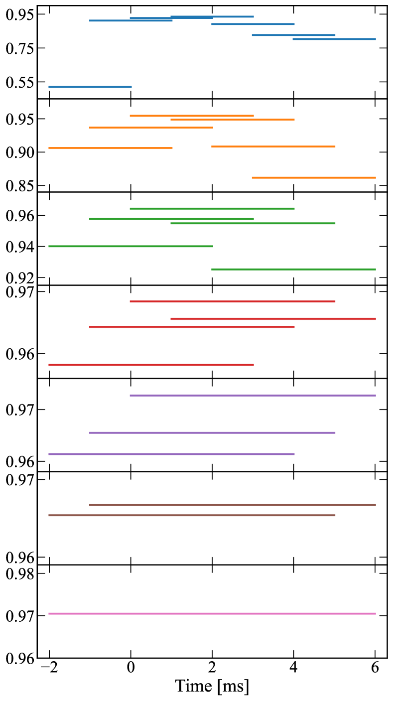
Figure 3: Classification accuracy of the Random Forest (RF) model across various signal lengths and locations, using a sliding window approach. Each signal is represented as a horizontal line, with its start and end points marking the signal’s duration. The sliding window progresses in 1 ms increments. The vertical position of each line corresponds to the classification accuracy value.

III Results

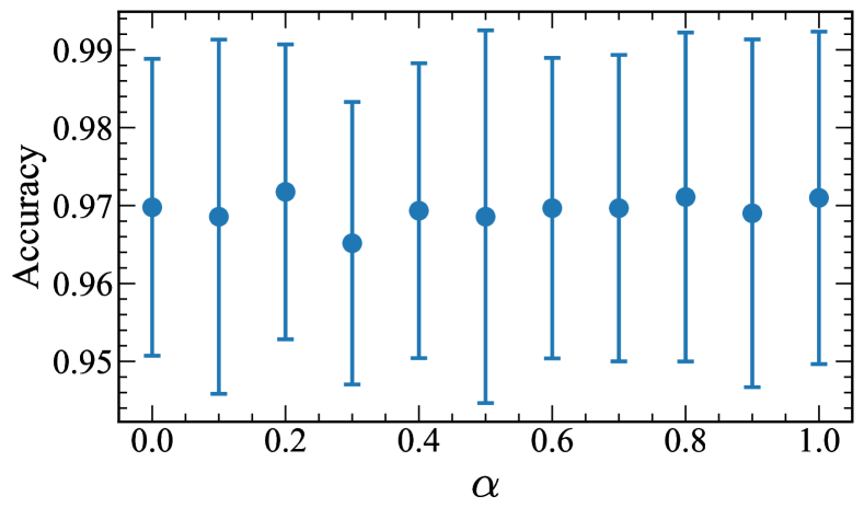
Figure 4: Classification accuracy of the EOS model as a function of the tapering parameter of the Tukey window. The dots represent the mean accuracy, and the error bars indicate the standard deviation.

Figure 1 shows the GW strain as a function of time for four different EOSs from $-2$ until $6$ ms after bounce. The variations between EOSs are approximately 5-10 %. Also shown is the signal for the SFHo EOS using the GREP approximation, which exhibits a similar 5-10 % variation but with a noticeably higher frequency due to the absence of time dilation in this approximation [67, 68]. The objective of the machine learning (ML) model is to distinguish the EOS of these signals. Unless stated otherwise, in the following we use the RF method for the time range of -2 to 6 ms, with a 10 kHz sampling rate.

III.1 Time range

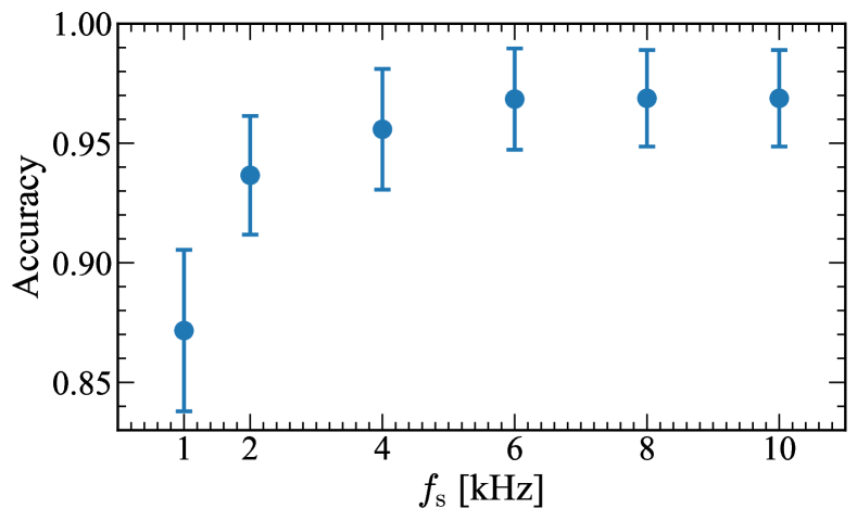
Figure 5: Classification accuracy of the EOS model as a function of the signal’s sampling frequency. The dots represent the mean accuracy, and the error bars indicate the standard deviation.

We first study the influence of the signal length and duration on the accuracy of the classifier using a sliding window approach. We consider signal lengths from 2 to 8 ms, with each length increasing in 1 ms increments. For each signal length, a sliding window moves across the entire signal in 1 ms steps. This is shown in Fig. 3, where each horizontal line represents a signal length and location in units of ms. The vertical position of each line corresponds to the classification accuracy value.

As we can see, accuracy varies with both signal length and location. For shorter signals, up to 5 ms, accuracy is more sensitive to the position of the window. This is because shorter windows do not capture the whole region that contains all key information. For example, for the signal from -2 to 0 ms, the classification accuracy is below 55 %, while for region from 0 to 2 ms, it raises to about 93 %. The highest accuracy of 94 % is achieved between 1 and 3 ms (cf. top panel of Fig. 3). This suggests that PNS oscillations in the early post-bounce phase carry the most inferrable information about the EOS.

In contrast, longer signals are less affected by window position, resulting in relatively stable accuracy across different signal locations. For the signal with the widest range from $-2$ to $6$ ms, we obtained accuracy of $96.8\pm 2.4\,\%$ (cf. bottom panel of Fig. 3). Note that this accuracy exceeds the 87 % reported in our previous work [65], as here we focus on waveforms with $0.02<T/|W|<0.18$, where distinguishing the EOS is easier.

In the following analysis, we use the entire signal from $-2$ to $6$ ms to ensure that the classifier has access to the maximum amount of information.

Table 4: Classification accuracy (mean $\pm$ standard deviation) in percentage (%) of various ML models on GR and GREP datasets. Each row shows the accuracy for the indicated dataset. GREP$\rightarrow$GR (GREP$\rightarrow$GR^∗) indicates training on the GREP dataset (with frequency normalization) and testing on GR, while GR$\rightarrow$GREP indicates the reverse. SVM shows the highest accuracy when trained and tested on the same dataset. All ML models trained on GREP data and tested on GR data (or vice versa) exhibit significantly lower accuracy. Values in bold highlight the best performance for each row.

Dataset	CNN	RNN	RF	SVM	NB	LR	$k$-NN	XGB
GR	97.4 $\pm$ 2.0	97.7 $\pm$ 1.9	96.8 $\pm$ 2.4	99.5 $\pm$ 1.0	48.9 $\pm$ 5.0	95.8 $\pm$ 2.1	93.8 $\pm$ 2.6	96.6 $\pm$ 2.3
GREP	97.2 $\pm$ 2.0	97.7 $\pm$ 1.8	96.2 $\pm$ 1.9	99.1 $\pm$ 1.0	56.2 $\pm$ 6.6	97.4 $\pm$ 2.0	91.2 $\pm$ 3.7	95.9 $\pm$ 2.3
GREP$\rightarrow$GR	37.9 $\pm$ 6.5	30.5 $\pm$ 5.5	35.2 $\pm$ 3.1	29.9 $\pm$ 2.5	38.8 $\pm$ 4.2	41.4 $\pm$ 3.1	33.1 $\pm$ 3.5	34.5 $\pm$ 3.1
GREP$\rightarrow$GR∗	62.0 $\pm$ 4.8	67.5 $\pm$ 5.2	43.6 $\pm$ 4.5	68.0 $\pm$ 4.3	36.4 $\pm$ 4.7	57.1 $\pm$ 4.8	57.8 $\pm$ 4.4	43.6 $\pm$ 4.6
GR$\rightarrow$GREP	25.9 $\pm$ 2.1	30.1 $\pm$ 6.0	26.0 $\pm$ 2.0	26.4 $\pm$ 2.0	45.4 $\pm$ 4.7	32.9 $\pm$ 3.2	27.3 $\pm$ 2.6	26.8 $\pm$ 3.1

III.2 Window function

Edwards (2017) [53] used a Tukey window to mitigate spectral leakage after downsampling the GW signal. In this section, we investigate the impact of the window on the classification accuracy. Fig. 4 shows the classification accuracy for varying $\alpha$, the tapering parameter of the Tukey window. As we can see, the accuracy is insensitive to $\alpha$. This can be attributed to the fact that, as indicated by the top panel in Fig. 3, all key information for EOS classification is concentrated in the middle part of the signal. Since the Tukey window primarily affects the tails, it has little impact on the classification accuracy.

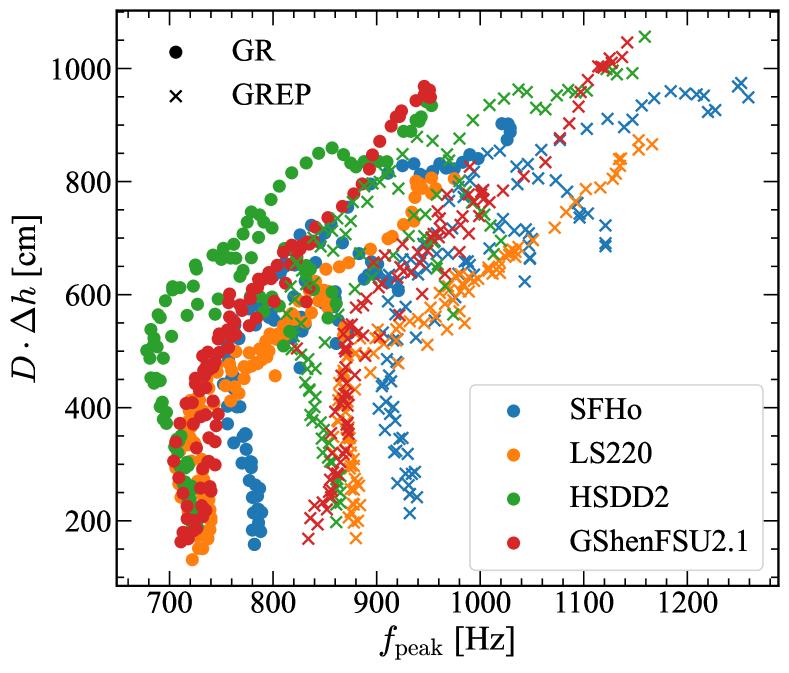
Figure 6: Relationship between the amplitude $D\cdot\Delta h$ and the peak frequency $f_{\mathrm{peak}}$ of the bounce GW signal for different EOSs (see [50] for definitions of these two quantities). The circles (crosses) correspond to GR (GREP) data. For a given $D\cdot\Delta h$, the values of $f_{\mathrm{peak}}$ are generally higher in the GREP dataset compared to GR. This is expected since GREP lacks the time dilation effect.

III.3 Sampling rate

Figure 5 shows the average classification accuracy as a function of the sampling frequency $f_{\mathrm{s}}$ of the signal. When the frequency exceeds $6\,\mathrm{kHz}$, the classification accuracy stabilizes at around $0.97$, becoming largely insensitive to further increases. This behavior is expected, as GW signals lack significant physical content above $\sim 6\,\mathrm{kHz}$ [e.g., 50]. This is consistent with our previous work [65], where a similar stabilization in accuracy was observed for sampling rates of 100 kHz, 10 kHz, and 5 kHz. However, for frequencies below $\sim 4\,\mathrm{kHz}$, the classification accuracy gradually declines, reaching about $0.87$ at $1\,\mathrm{kHz}$, suggesting that some of EOS-specific information lies outside this sampling rate. In the following, we use the signal with $10\,\mathrm{kHz}$ sampling rate.

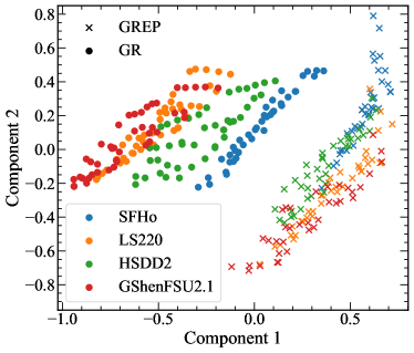
(a)

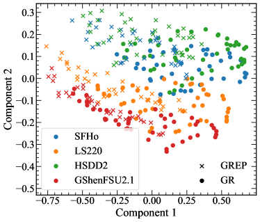
(b)

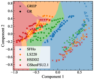
(c)

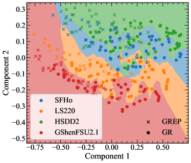
(d)

Figure 7: Visualization of the first two principal components of the GR and GREP datasets. The panels display the distribution of waveforms for the original dataset (left) and the time-normalized dataset (right). In the left panel, the GR data (circles) and GREP data (crosses) are clearly separated and form distinct groups. However, in the right panel, after time normalization, this distinction fades, and the data points cluster based on the equation of state (EOS), rather than the method (GR or GREP). The bottom panels show the decision boundaries formed by the $k$-NN algorithm, with GR used for training and GREP for testing. The colored regions (blue for SFHo, orange for LS220, green for HSDD2, and red for GShenFSU2.1) indicate the classification regions.

III.4 ML models

Table 4 presents the classification accuracy results across different ML models. Each entry in the table represents the mean accuracy and the corresponding standard deviation.

The SVM model consistently outperforms other models, achieving the highest mean accuracy of 99.5% ± 1.0%. The strong performance of the SVM model is likely due to its configuration and the nature of the GW data. The polynomial kernel with a degree of 4 allows the SVM to capture complex, non-linear relationships necessary for classifying different EOSs. The regularization parameter $C=10$ effectively balances the decision boundary margin with a controlled level of misclassification, enhancing the model’s ability to generalize without overfitting. These factors together likely contribute to the SVM model’s high classification accuracy.

Along with SVM, both RNN and CNN achieve strong performance, with average accuracies surpassing 97 %. RF, XGB, LR, and k-NN exhibit slightly lower but still high average accuracies of 96.8, 96.6, 95.8, 93.8, respectively (cf. Table 4). In contrast, Naïve Bayes shows a significantly lower accuracy of $48.9\pm 5\,\%$, primarily due to its assumption of feature independence, which overlooks the correlations and temporal patterns that exist in time series data. Overall, except for Naïve Bayes, all models demonstrate strong performance in this classification task.

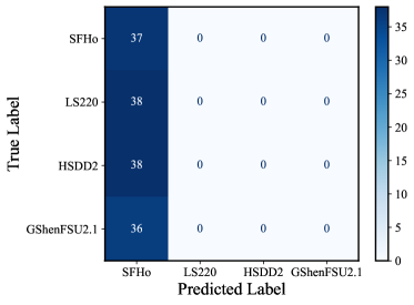
(a)

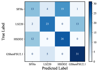
(b)

Figure 8: Confusion matrices illustrating the performance of the $k$-NN algorithm in classifying GREP data when trained on GR data. The left panel shows the confusion matrix for the original dataset. The right panel displays the confusion matrix after frequency normalization. In the original dataset, substantial misclassifications, particularly as SFHo, result in lower classification accuracy of $\sim 25\,\%$. After frequency normalization, accuracy improves to $\sim 62\,\%$.

III.5 GR vs effective potential

Next, we assess the ability of ML models trained on GREP data to classify the EOS from realistic GW signals, which are obtained from GW simulations. While all ML methods discussed in this paper were applied, for brevity and the reasons outlined below, we focus on the results obtained with the $k$-NN method.

The model trained and tested on GREP data achieves an accuracy of $91.2\pm 3.7\%$, which is comparable to the $93.8\pm 2.6\%$ accuracy obtained for the model trained and tested on GR data. However, when the model trained on GREP data is used to classify the GR data, the accuracy drops to $33.1\pm 3.5\%$, and similarly, the model trained on the GR data classifies the GREP signals with only $27.3\pm 2.6\%$ accuracy. This is expected, as GREP and GR waveforms differ by $\sim$ 5-10$\,\%$, which is of the same order as the difference between different EOSs, as can be gleaned from Fig. 1. For this reason, the model trained on GREP (GR) struggles to classify GR (GREP) signals.

Another factor contributing to the lower accuracy is the frequency difference. Since GREP lacks the time dilation effect, it produces dynamics with higher frequencies [68]. This is evident in Fig. 6, which plots the GW amplitude $D\cdot\Delta h$ against the peak frequency $f_{\mathrm{peak}}$ for both GR and GREP datasets (see [50] for definitions of these two quantities). As we can see, the GREP waveforms have $\sim 15\,\%$ higher frequencies compared to the GR models.

To gain deeper insight, we design a simple experiment. We select waveforms with $T/|W|$ below 0.06, where the amplitude-normalized waveforms are similar to each other [50]. We then generate another dataset by normalizing time by $f_{\mathrm{peak}}$, as done in [88]. Next, we apply Principal Component Analysis (PCA) to reduce the dimensionality of the waveforms in both datasets from 81 to 2. We then analyze the resulting data.

The upper panel of Fig. 7 shows each waveform as the first two principal components. The left panel corresponds to the original dataset, while the right panel corresponds to the time-normalized dataset. In the left panel, the GR and GREP data points are distinctly grouped and clearly separated from each other. In contrast, the right panel demonstrates that after the temporal normalizing, the distinction between GR and GREP becomes less pronounced and the data points cluster into somewhat distinct groups based on their EOSs.

We apply the $k$-Nearest Neighbors algorithm to gain a deeper understanding of the impact of the temporal normalization. The blue, orange, green, and red regions in the bottom panels of Fig. 7 correspond to the SFHo, LS220, HSDD2, and GShenFSU2.1 EOSs, respectively. These regions represent the decision boundaries formed by the $k$-NN model. Any point within this region will be classified according to the EOS associated with that region. Most GR points fall within the decision boundaries of their respective EOSs. In contrast, all GREP points are located within the regions corresponding to the SFHo EOS for the GR data, meaning all GREP signals will be classified as SFHo. However, the time-normalized GREP data points, shown in the right panel, align better with the decision boundaries. Thus improves classification accuracy to $\sim 60\,\%$. Despite this, the accuracy remains substantially lower than the $93.8\pm 2.6\,\%$ achieved when using GR data for both training and testing.

The left and right panels of Fig. 8 show the corresponding confusion matrices for the original and time-normalized data. For the original data, all GREP points fall within the SFHo EOS region of the GR data, leading to their classification as SFHo (left panel). The precision and recall for SFHo are $\sim$ 0.25 and 1, respectively. For all other EOSs, precision is undefined due to the division by zero, while recall is equal to zero. For the time-normalized data (right panel), GShenFSU2.1 has the highest recall and precision, making it the best-classified EOS, while SFHo performs the worst. Notably, SFHo is often misclassified as HSDD2.

To verify the robustness, we conduct a similar test on the full data without applying the PCA reduction. We achieve a comparable accuracy. The accuracy of all ML models is provided in Table 4. These results indicate that the time normalization partially mitigates the absence of time dilation effects in GREP, leading to improved classification accuracy. However, even the best-performing model, SVM, reaches only $68.0\pm 4.3\,\%$ accuracy. This suggests that GREP waveforms lack the precision required to capture subtle EOS-related features.

IV Conclusion

In this study, we evaluated the impact of various machine learning models, parameter configurations, and data preprocessing techniques on the accuracy of equation-of-state (EOS) classification using bounce gravitational wave (GW) data from rotating core-collapse supernovae.

As expected, we find that the signal length has a significant impact on accuracy: longer signals provide more information, enhancing the model’s ability to classify accurately (cf. Section III.1 for details). Applying a Tukey window has little impact on classification accuracy, as most EOS-sensitive information is concentrated in the middle part of the signal, while the window primarily affects the signal’s tails (cf. Section III.2). We find that the sampling frequency does not influence accuracy as long as it exceeds 6 kHz or above, which is unsurprising since the GW signal lacks substantial components at these or higher frequencies (cf. Section III.3 for details).

Our results show that Support Vector Machines (SVM), Recurrent Neural Networks (RNN), and Convolutional Neural Networks (CNN) achieve the highest classification accuracy, exceeding 97 % for a set of four EOSs. Random Forest (RF), XGBoost (XGB), Logistic Regression (LR), and $k$-Nearest Neighbors ($k$-NN) also perform well, with average accuracies of 96.8 %, 96.6 %, 95.8 %, and 93.8 %, respectively. In contrast, the Naïve Bayes method demonstrates the lowest accuracy, falling below 50 % (cf. Section III.4 for details).

We also assess the impact of approximating the gravitational wave (GW) signal using the general relativistic effect potential (GREP) on classification performance. Models trained on GREP data classify waveforms based on general relativity (GR) with an average accuracy of approximately 35 %, which is significantly lower than the over 90 % accuracy achieved by models trained on GR signals. This outcome is expected, as GREP can approximate GR gravity but does not capture other relativistic effects, such as time dilation, leading to a generally higher frequency in GREP. However, when the GW signal is normalized by the peak GW frequency, the classification accuracy improves substantially, but still remains below 70 % (cf. Section III.5 for details). This suggests that the GREP approximation produces waveforms lacking the precision necessary to capture subtle signal characteristics, such as the EOS.

Our work has a number of limitations. In particular, we consider only one progenitor model. While different progenitors are expected to produce similar bounce GW signals for the same angular momentum distribution [44], variations of a few percent can still occur. Moreover, we do not include detector noise. Both factors may interfere with the ML models’ ability to identify the EOS. We will address these issues in future work.

DATA AVAILABILITY

The gravitational waveforms are publicly accessible at https://doi.org/10.5281/zenodo.13774509.

Appendix A General relativistic effective potential

The GR effective potential is obtained by replacing the spherically symmetric part ${\bar{\Phi}}$ of the Newtonian potential $\Phi$ with the relativistic Tolman-Oppenheimer-Volkoff (TOV) solution ${\bar{\Phi}}_{\mathrm{TOV}}$ [89, 66]:

$$\Phi_{\mathrm{GREP}}=\Phi-{\bar{\Phi}}+{\bar{\Phi}}_{\mathrm{TOV}}.$$ (1)

The TOV potential is obtained as

$${\bar{\Phi}}_{\mathrm{TOV}}=\int_{\infty}^{r}\left[{m}_{\mathrm{TOV}}+4\pi r^{\prime 3}\left(P+P_{\nu}\right)\right]\frac{h}{\Gamma^{2}}\frac{dr^{\prime}}{r^{\prime 2}},$$ (2)

where $h=1+\epsilon+P/\rho$ is the specific enthalpy, $\epsilon$ is the specific internal energy, $P$ is pressure, and $P_{\nu}$ is the neutrino pressure. Parameter $\Gamma$ is given by

$$\Gamma=\left(1+\upsilon_{r}^{2}-\frac{2m_{\mathrm{TOV}}}{r}\right)^{0.5},$$ (3)

where $\upsilon_{r}$ is the angle-averaged radial velocity. Following [67], we define the enclosed mass as

$$m_{\mathrm{TOV}}=4\pi\int_{0}^{r}\left(\rho+\rho\epsilon+E_{\nu}+\frac{\upsilon_{i}F^{i}_{\nu}}{\Gamma}\right)\Gamma r^{\prime 2}dr^{\prime}.$$ (4)

This choice of $m_{\mathrm{TOV}}$, referred to as ”case A”, was found to better reproduce exact GR results [67]. Here, $E_{\nu}$ and $F_{\nu}$ and the energy and momentum density of neutrinos. Since the $Y_{e}(\rho)$ deleptonization scheme we employ does not explicitly evolve the neuntiro momentum density [77], we set it to zero in both GR and GREP versions of the code. Since parameter $\Gamma$ depends on $m_{\mathrm{TOV}}$ and vice versa, we can obtain these quantities either by solving equations (3) and (4) iteratively [90] or through ODE integration [68].

This method relies on the spherically symmetric component of the GR potential, but because rotation breaks this symmetry, its accuracy may decrease with increasing rotation. Rotational corrections, as suggested by Müller et al. [68] and recently used in Müller and Varma [91], Varma et al. [92], can partially mitigate the issue. However, these corrections have not been implemented in our work, as our goal is to investigate the most commonly used formulation of GREP found in the literature.

References

- Abbott et al. [2016] B. P. Abbott, R. Abbott, T. Abbott, M. Abernathy, F. Acernese, K. Ackley, C. Adams, T. Adams, P. Addesso, R. Adhikari, et al., GW150914: The Advanced LIGO detectors in the era of first discoveries, Physical review letters 116, 131103 (2016).
- Abbott et al. [2017] B. P. Abbott, R. Abbott, T. Abbott, F. Acernese, K. Ackley, C. Adams, T. Adams, P. Addesso, R. X. Adhikari, V. B. Adya, et al., GW170817: observation of gravitational waves from a binary neutron star inspiral, Physical review letters 119, 161101 (2017).
- Abbott et al. [2021] R. Abbott, T. D. Abbott, S. Abraham, F. Acernese, K. Ackley, A. Adams, C. Adams, R. Adhikari, V. Adya, C. Affeldt, et al., Observation of gravitational waves from two neutron star–black hole coalescences, The Astrophysical journal letters 915, L5 (2021).
- Kotake [2013] K. Kotake, Multiple physical elements to determine the gravitational-wave signatures of core-collapse supernovae, Comptes Rendus Physique 14, 318 (2013), arXiv:1110.5107 [astro-ph.HE] .
- Hayama et al. [2018] K. Hayama, T. Kuroda, K. Kotake, and T. Takiwaki, Circular polarization of gravitational waves from non-rotating supernova cores: a new probe into the pre-explosion hydrodynamics, MNRAS 477, L96 (2018), arXiv:1802.03842 [astro-ph.HE] .
- Schneider et al. [2019] A. S. Schneider, L. F. Roberts, C. D. Ott, and E. O’Connor, Equation of state effects in the core collapse of a 20 -M⊙ star, Phys. Rev. C 100, 055802 (2019), arXiv:1906.02009 [astro-ph.HE] .
- Abbott et al. [2020] B. Abbott, R. Abbott, T. Abbott, S. Abraham, F. Acernese, K. Ackley, C. Adams, V. Adya, C. Affeldt, M. Agathos, et al., Optically targeted search for gravitational waves emitted by core-collapse supernovae during the first and second observing runs of advanced ligo and advanced virgo, Physical Review D 101, 084002 (2020).
- Szczepańczyk et al. [2024] M. J. Szczepańczyk, Y. Zheng, J. M. Antelis, M. Benjamin, M.-A. Bizouard, A. Casallas-Lagos, P. Cerdá-Durán, et al., Optically targeted search for gravitational waves emitted by core-collapse supernovae during the third observing run of Advanced LIGO and Advanced Virgo, Phys. Rev. D 110, 042007 (2024), arXiv:2305.16146 [astro-ph.HE] .
- Powell and Müller [2022] J. Powell and B. Müller, Inferring astrophysical parameters of core-collapse supernovae from their gravitational-wave emission, Phys. Rev. D 105, 063018 (2022), arXiv:2201.01397 [astro-ph.HE] .
- Gossan et al. [2016] S. E. Gossan, P. Sutton, A. Stuver, M. Zanolin, K. Gill, and C. D. Ott, Observing gravitational waves from core-collapse supernovae in the advanced detector era, Phys. Rev. D 93, 042002 (2016), arXiv:1511.02836 [astro-ph.HE] .
- Adams et al. [2013] S. M. Adams, C. S. Kochanek, J. F. Beacom, M. R. Vagins, and K. Z. Stanek, Observing the Next Galactic Supernova, Astrophys. J. 778, 164 (2013), arXiv:1306.0559 [astro-ph.HE] .
- Srivastava et al. [2019] V. Srivastava, S. Ballmer, D. A. Brown, C. Afle, A. Burrows, D. Radice, and D. Vartanyan, Detection prospects of core-collapse supernovae with supernova-optimized third-generation gravitational-wave detectors, Phys. Rev. D 100, 043026 (2019), arXiv:1906.00084 [gr-qc] .
- O’Connor and Ott [2011] E. O’Connor and C. D. Ott, Black Hole Formation in Failing Core-Collapse Supernovae, Astrophys. J. 730, 70 (2011), arXiv:1010.5550 [astro-ph.HE] .
- Cerdá-Durán et al. [2013] P. Cerdá-Durán, N. DeBrye, M. A. Aloy, J. A. Font, and M. Obergaulinger, Gravitational Wave Signatures in Black Hole Forming Core Collapse, ApJL 779, L18 (2013), arXiv:1310.8290 [astro-ph.SR] .
- Burrows et al. [2023] A. Burrows, D. Vartanyan, and T. Wang, Black Hole Formation Accompanied by the Supernova Explosion of a 40 M ⊙ Progenitor Star, Astrophys. J. 957, 68 (2023), arXiv:2308.05798 [astro-ph.SR] .
- Janka et al. [2016] H.-T. Janka, T. Melson, and A. Summa, Physics of Core-Collapse Supernovae in Three Dimensions: A Sneak Preview, Annual Review of Nuclear and Particle Science 66, 341 (2016), arXiv:1602.05576 [astro-ph.SR] .
- Burrows [2013] A. Burrows, Colloquium: Perspectives on core-collapse supernova theory, Reviews of Modern Physics 85, 245 (2013), arXiv:1210.4921 [astro-ph.SR] .
- Müller [2020] B. Müller, Hydrodynamics of core-collapse supernovae and their progenitors, Living Reviews in Computational Astrophysics 6, 3 (2020), arXiv:2006.05083 [astro-ph.SR] .
- Mezzacappa et al. [2020] A. Mezzacappa, E. Endeve, O. E. B. Messer, and S. W. Bruenn, Physical, numerical, and computational challenges of modeling neutrino transport in core-collapse supernovae, Living Reviews in Computational Astrophysics 6, 4 (2020), arXiv:2010.09013 [astro-ph.HE] .
- O’Connor and Ott [2013] E. O’Connor and C. D. Ott, The Progenitor Dependence of the Pre-explosion Neutrino Emission in Core-collapse Supernovae, Astrophys. J. 762, 126 (2013), arXiv:1207.1100 [astro-ph.HE] .
- Müller and Janka [2014] B. Müller and H.-T. Janka, A New Multi-dimensional General Relativistic Neutrino Hydrodynamics Code for Core-collapse Supernovae. IV. The Neutrino Signal, Astrophys. J. 788, 82 (2014), arXiv:1402.3415 [astro-ph.SR] .
- Lentz et al. [2012] E. J. Lentz, A. Mezzacappa, O. E. B. Messer, W. R. Hix, and S. W. Bruenn, Interplay of Neutrino Opacities in Core-collapse Supernova Simulations, Astrophys. J. 760, 94 (2012), arXiv:1206.1086 [astro-ph.SR] .
- Müller et al. [2012] B. Müller, H.-T. Janka, and A. Marek, A New Multi-dimensional General Relativistic Neutrino Hydrodynamics Code for Core-collapse Supernovae. II. Relativistic Explosion Models of Core-collapse Supernovae, Astrophys. J. 756, 84 (2012), arXiv:1202.0815 [astro-ph.SR] .
- Herant et al. [1994] M. Herant, W. Benz, W. R. Hix, C. L. Fryer, and S. A. Colgate, Inside the Supernova: A Powerful Convective Engine, Astrophys. J. 435, 339 (1994), arXiv:astro-ph/9404024 [astro-ph] .
- Burrows et al. [1995] A. Burrows, J. Hayes, and B. A. Fryxell, On the Nature of Core-Collapse Supernova Explosions, Astrophys. J. 450, 830 (1995), arXiv:astro-ph/9506061 [astro-ph] .
- Janka and Mueller [1995] H. T. Janka and E. Mueller, The First Second of a Type II Supernova: Convection, Accretion, and Shock Propagation, Astrophys. J. 448, L109 (1995), arXiv:astro-ph/9503015 [astro-ph] .
- Blondin et al. [2003] J. M. Blondin, A. Mezzacappa, and C. DeMarino, Stability of Standing Accretion Shocks, with an Eye toward Core-Collapse Supernovae, Astrophys. J. 584, 971 (2003), arXiv:astro-ph/0210634 [astro-ph] .
- Foglizzo et al. [2006] T. Foglizzo, L. Scheck, and H. T. Janka, Neutrino-driven Convection versus Advection in Core-Collapse Supernovae, Astrophys. J. 652, 1436 (2006), arXiv:astro-ph/0507636 [astro-ph] .
- Burrows et al. [2007] A. Burrows, L. Dessart, E. Livne, C. D. Ott, and J. Murphy, Simulations of Magnetically Driven Supernova and Hypernova Explosions in the Context of Rapid Rotation, Astrophys. J. 664, 416 (2007), arXiv:astro-ph/0702539 .
- Winteler et al. [2012] C. Winteler, R. Käppeli, A. Perego, A. Arcones, N. Vasset, N. Nishimura, M. Liebendörfer, and F. K. Thielemann, Magnetorotationally Driven Supernovae as the Origin of Early Galaxy r-process Elements?, ApJL 750, L22 (2012), arXiv:1203.0616 [astro-ph.SR] .
- Mösta et al. [2014] P. Mösta, S. Richers, C. D. Ott, R. Haas, A. L. Piro, K. Boydstun, E. Abdikamalov, C. Reisswig, and E. Schnetter, Magnetorotational Core-collapse Supernovae in Three Dimensions, ApJL 785, L29 (2014), arXiv:1403.1230 [astro-ph.HE] .
- Obergaulinger and Aloy [2020] M. Obergaulinger and M. Á. Aloy, Magnetorotational core collapse of possible GRB progenitors - I. Explosion mechanisms, MNRAS 492, 4613 (2020), arXiv:1909.01105 [astro-ph.HE] .
- Kuroda et al. [2020] T. Kuroda, A. Arcones, T. Takiwaki, and K. Kotake, Magnetorotational Explosion of a Massive Star Supported by Neutrino Heating in General Relativistic Three-dimensional Simulations, Astrophys. J. 896, 102 (2020), arXiv:2003.02004 [astro-ph.HE] .
- Woosley and Bloom [2006] S. E. Woosley and J. S. Bloom, The Supernova Gamma-Ray Burst Connection, Annual Review of Astronomy and Astrophysics 44, 507 (2006), arXiv:astro-ph/0609142 [astro-ph] .
- Woosley and Heger [2006] S. E. Woosley and A. Heger, The Progenitor Stars of Gamma-Ray Bursts, Astrophys. J. 637, 914 (2006), arXiv:astro-ph/0508175 [astro-ph] .
- Metzger et al. [2011] B. D. Metzger, D. Giannios, T. A. Thompson, N. Bucciantini, and E. Quataert, The protomagnetar model for gamma-ray bursts, MNRAS 413, 2031 (2011), arXiv:1012.0001 [astro-ph.HE] .
- Abdikamalov et al. [2022] E. Abdikamalov, G. Pagliaroli, and D. Radice, Gravitational Waves from Core-Collapse Supernovae, in Handbook of Gravitational Wave Astronomy, edited by C. Bambi, S. Katsanevas, and K. D. Kokkotas (2022) p. 21.
- Mezzacappa and Zanolin [2024] A. Mezzacappa and M. Zanolin, Gravitational Waves from Neutrino-Driven Core Collapse Supernovae: Predictions, Detection, and Parameter Estimation, arXiv e-prints , arXiv:2401.11635 (2024), arXiv:2401.11635 [astro-ph.HE] .
- Murphy et al. [2009] J. W. Murphy, C. D. Ott, and A. Burrows, A Model for Gravitational Wave Emission from Neutrino-Driven Core-Collapse Supernovae, Astrophys. J. 707, 1173 (2009), arXiv:0907.4762 [astro-ph.SR] .
- Radice et al. [2019] D. Radice, V. Morozova, A. Burrows, D. Vartanyan, and H. Nagakura, Characterizing the Gravitational Wave Signal from Core-collapse Supernovae, ApJL 876, L9 (2019), arXiv:1812.07703 [astro-ph.HE] .
- Andresen et al. [2017] H. Andresen, B. Müller, E. Müller, and H. T. Janka, Gravitational wave signals from 3D neutrino hydrodynamics simulations of core-collapse supernovae, MNRAS 468, 2032 (2017), arXiv:1607.05199 [astro-ph.HE] .
- Mezzacappa et al. [2023] A. Mezzacappa, P. Marronetti, R. E. Landfield, E. J. Lentz, R. D. Murphy, W. Raphael Hix, J. A. Harris, S. W. Bruenn, J. M. Blondin, O. E. Bronson Messer, J. Casanova, and L. L. Kronzer, Core collapse supernova gravitational wave emission for progenitors of 9.6, 15, and 25M, Phys. Rev. D 107, 043008 (2023), arXiv:2208.10643 [astro-ph.SR] .
- Vartanyan et al. [2023] D. Vartanyan, A. Burrows, T. Wang, M. S. B. Coleman, and C. J. White, Gravitational-wave signature of core-collapse supernovae, Phys. Rev. D 107, 103015 (2023), arXiv:2302.07092 [astro-ph.HE] .
- Ott et al. [2012] C. D. Ott, E. Abdikamalov, E. O’Connor, C. Reisswig, R. Haas, P. Kalmus, S. Drasco, A. Burrows, and E. Schnetter, Correlated gravitational wave and neutrino signals from general-relativistic rapidly rotating iron core collapse, Phys. Rev. D 86, 024026 (2012), arXiv:1204.0512 [astro-ph.HE] .
- Müller et al. [2013] B. Müller, H.-T. Janka, and A. Marek, A New Multi-dimensional General Relativistic Neutrino Hydrodynamics Code of Core-collapse Supernovae. III. Gravitational Wave Signals from Supernova Explosion Models, Astrophys. J. 766, 43 (2013), arXiv:1210.6984 [astro-ph.SR] .
- Morozova et al. [2018] V. Morozova, D. Radice, A. Burrows, and D. Vartanyan, The Gravitational Wave Signal from Core-collapse Supernovae, Astrophys. J. 861, 10 (2018), arXiv:1801.01914 [astro-ph.HE] .
- Pajkos et al. [2019] M. A. Pajkos, S. M. Couch, K.-C. Pan, and E. P. O’Connor, Features of Accretion-phase Gravitational-wave Emission from Two-dimensional Rotating Core-collapse Supernovae, Astrophys. J. 878, 13 (2019), arXiv:1901.09055 [astro-ph.HE] .
- Pajkos et al. [2021] M. A. Pajkos, M. L. Warren, S. M. Couch, E. P. O’Connor, and K.-C. Pan, Determining the Structure of Rotating Massive Stellar Cores with Gravitational Waves, Astrophys. J. 914, 80 (2021), arXiv:2011.09000 [astro-ph.HE] .
- Powell et al. [2024] J. Powell, A. Iess, M. Llorens-Monteagudo, M. Obergaulinger, B. Müller, A. Torres-Forné, E. Cuoco, and J. A. Font, Determining the core-collapse supernova explosion mechanism with current and future gravitational-wave observatories, Phys. Rev. D 109, 063019 (2024), arXiv:2311.18221 [astro-ph.HE] .
- Richers et al. [2017] S. Richers, C. D. Ott, E. Abdikamalov, E. O’Connor, and C. Sullivan, Equation of state effects on gravitational waves from rotating core collapse, Phys. Rev. D 95, 063019 (2017), arXiv:1701.02752 [astro-ph.HE] .
- Wolfe et al. [2023] N. E. Wolfe, C. Fröhlich, J. M. Miller, A. Torres-Forné, and P. Cerdá-Durán, Gravitational Wave Eigenfrequencies from Neutrino-driven Core-collapse Supernovae, Astrophys. J. 954, 161 (2023), arXiv:2303.16962 [astro-ph.HE] .
- Powell and Müller [2024] J. Powell and B. Müller, The gravitational-wave emission from the explosion of a 15 solar mass star with rotation and magnetic fields, MNRAS 532, 4326 (2024), arXiv:2406.09691 [astro-ph.HE] .
- Edwards [2021] M. C. Edwards, Classifying the equation of state from rotating core collapse gravitational waves with deep learning, Phys. Rev. D 103, 024025 (2021), arXiv:2009.07367 [astro-ph.IM] .
- Chao et al. [2022] Y.-S. Chao, C.-Z. Su, T.-Y. Chen, D.-W. Wang, and K.-C. Pan, Determining the Core Structure and Nuclear Equation of State of Rotating Core-collapse Supernovae with Gravitational Waves by Convolutional Neural Networks, Astrophys. J. 939, 13 (2022), arXiv:2209.10089 [astro-ph.HE] .
- Astone et al. [2018] P. Astone, P. Cerdá-Durán, I. Di Palma, M. Drago, F. Muciaccia, C. Palomba, and F. Ricci, New method to observe gravitational waves emitted by core collapse supernovae, Phys. Rev. D 98, 122002 (2018).
- Chan et al. [2020] M. L. Chan, I. S. Heng, and C. Messenger, Detection and classification of supernova gravitational wave signals: A deep learning approach, Phys. Rev. D 102, 043022 (2020).
- Iess et al. [2020] A. Iess, E. Cuoco, F. Morawski, and J. Powell, Core-collapse supernova gravitational-wave search and deep learning classification, Machine Learning: Science and Technology 1, 025014 (2020).
- López et al. [2021] M. López, I. Di Palma, M. Drago, P. Cerdá-Durán, and F. Ricci, Deep learning for core-collapse supernova detection, Phys. Rev. D 103, 063011 (2021).
- Antelis et al. [2022] J. M. Antelis, M. Cavaglia, T. Hansen, M. D. Morales, C. Moreno, S. Mukherjee, M. J. Szczepańczyk, and M. Zanolin, Using supervised learning algorithms as a follow-up method in the search of gravitational waves from core-collapse supernovae, Phys. Rev. D 105, 084054 (2022), arXiv:2111.07219 [gr-qc] .
- Saiz-Pérez et al. [2022] A. Saiz-Pérez, A. Torres-Forné, and J. A. Font, Classification of core-collapse supernova explosions with learned dictionaries, MNRAS 512, 3815 (2022), arXiv:2110.12941 [gr-qc] .
- Mitra et al. [2023] A. Mitra, B. Shukirgaliyev, Y. S. Abylkairov, and E. Abdikamalov, Exploring supernova gravitational waves with machine learning, MNRAS 520, 2473 (2023), arXiv:2209.14542 [astro-ph.HE] .
- Eccleston and Edwards [2024] T. Eccleston and M. C. Edwards, A generative adversarial network for stellar core-collapse gravitational-waves, arXiv e-prints , arXiv:2408.02895 (2024), arXiv:2408.02895 [gr-qc] .
- Morales et al. [2024] M. D. Morales, J. M. Antelis, and C. Moreno, Residual neural networks to classify the high frequency emission in core-collapse supernova gravitational waves, arXiv e-prints , arXiv:2406.00422 (2024), arXiv:2406.00422 [astro-ph.HE] .
- Nunes et al. [2024] S. Nunes, G. Escrig, O. G. Freitas, J. A. Font, T. Fernandes, A. Onofre, and A. Torres-Forné, Deep-Learning Classification and Parameter Inference of Rotational Core-Collapse Supernovae, arXiv e-prints , arXiv:2403.04938 (2024), arXiv:2403.04938 [astro-ph.HE] .
- Mitra et al. [2024] A. Mitra, D. Orel, Y. S. Abylkairov, B. Shukirgaliyev, and E. Abdikamalov, Probing nuclear physics with supernova gravitational waves and machine learning, MNRAS 529, 3582 (2024), arXiv:2310.15649 [astro-ph.HE] .
- Rampp and Janka [2002] M. Rampp and H. T. Janka, Radiation hydrodynamics with neutrinos. Variable Eddington factor method for core-collapse supernova simulations, A&A 396, 361 (2002), arXiv:astro-ph/0203101 [astro-ph] .
- Marek et al. [2006] A. Marek, H. Dimmelmeier, H.-T. Janka, E. Müller, and R. Buras, Exploring the relativistic regime with Newtonian hydrodynamics: an improved effective gravitational potential for supernova simulations, A&A 445, 273 (2006), arXiv:astro-ph/0502161 .
- Müller et al. [2008] B. Müller, H. Dimmelmeier, and E. Müller, Exploring the relativistic regime with Newtonian hydrodynamics. II. An effective gravitational potential for rapid rotation, A&A 489, 301 (2008).
- Dimmelmeier et al. [2002] H. Dimmelmeier, J. A. Font, and E. Müller, Relativistic simulations of rotational core collapse I. Methods, initial models, and code tests, A&A 388, 917 (2002), arXiv:astro-ph/0204288 [astro-ph] .
- Dimmelmeier et al. [2005] H. Dimmelmeier, J. Novak, J. A. Font, J. M. Ibáñez, and E. Müller, Combining spectral and shock-capturing methods: A new numerical approach for 3D relativistic core collapse simulations, Phys. Rev. D 71, 064023 (2005), astro-ph/0407174 .
- Isenberg [2008] J. A. Isenberg, Waveless approximation theories of gravity, International Journal of Modern Physics D 17, 265 (2008), https://doi.org/10.1142/S0218271808011997 .
- Wilson et al. [1996] J. R. Wilson, G. J. Mathews, and P. Marronetti, Relativistic numerical model for close neutron-star binaries, Phys. Rev. D 54, 1317 (1996), arXiv:gr-qc/9601017 [gr-qc] .
- Cordero-Carrión et al. [2009] I. Cordero-Carrión, P. Cerdá-Durán, H. Dimmelmeier, J. L. Jaramillo, J. Novak, and E. Gourgoulhon, Improved constrained scheme for the Einstein equations: An approach to the uniqueness issue, Phys. Rev. D 79, 024017 (2009), arXiv:0809.2325 [gr-qc] .
- Cerdá-Durán et al. [2005] P. Cerdá-Durán, G. Faye, H. Dimmelmeier, J. A. Font, J. M. Ibáñez, E. Müller, and G. Schäfer, CFC+: improved dynamics and gravitational waveforms from relativistic core collapse simulations, A&A 439, 1033 (2005), arXiv:astro-ph/0412611 [astro-ph] .
- Shibata and Sekiguchi [2004] M. Shibata and Y.-I. Sekiguchi, Gravitational waves from axisymmetric rotating stellar core collapse to a neutron star in full general relativity, Phys. Rev. D 69, 084024 (2004), arXiv:gr-qc/0402040 [gr-qc] .
- Ott et al. [2007] C. D. Ott, H. Dimmelmeier, A. Marek, H. T. Janka, B. Zink, I. Hawke, and E. Schnetter, Rotating collapse of stellar iron cores in general relativity, Classical and Quantum Gravity 24, S139 (2007), arXiv:astro-ph/0612638 [astro-ph] .
- Liebendörfer et al. [2005] M. Liebendörfer, M. Rampp, H.-T. Janka, and A. Mezzacappa, Supernova Simulations with Boltzmann Neutrino Transport: A Comparison of Methods, Astrophys. J. 620, 840 (2005), arXiv:astro-ph/0310662 .
- O’Connor [2015] E. O’Connor, An Open-source Neutrino Radiation Hydrodynamics Code for Core-collapse Supernovae, Astrophys. J. Suppl. S. 219, 24 (2015), arXiv:1411.7058 [astro-ph.HE] .
- Steiner et al. [2013] A. W. Steiner, M. Hempel, and T. Fischer, Core-collapse Supernova Equations of State Based on Neutron Star Observations, Astrophys. J. 774, 17 (2013), arXiv:1207.2184 [astro-ph.SR] .
- Lattimer and Swesty [1991] J. M. Lattimer and F. D. Swesty, A generalized equation of state for hot, dense matter, Nucl. Phys. A 535, 331 (1991).
- Shen et al. [2011] G. Shen, C. J. Horowitz, and E. O’Connor, Second relativistic mean field and virial equation of state for astrophysical simulations, Phys. Rev. C 83, 065808 (2011).
- Hempel and Schaffner-Bielich [2010] M. Hempel and J. Schaffner-Bielich, A statistical model for a complete supernova equation of state, Nucl. Phys. A 837, 210 (2010), arXiv:0911.4073 [nucl-th] .
- Hempel et al. [2012] M. Hempel, T. Fischer, J. Schaffner-Bielich, and M. Liebendörfer, New Equations of State in Simulations of Core-collapse Supernovae, Astrophys. J. 748, 70 (2012), arXiv:1108.0848 [astro-ph.HE] .
- Woosley and Heger [2007] S. E. Woosley and A. Heger, Nucleosynthesis and remnants in massive stars of solar metallicity, Physics Reports 442, 269 (2007), arXiv:astro-ph/0702176 [astro-ph] .
- Abdikamalov et al. [2014] E. Abdikamalov, S. Gossan, A. M. DeMaio, and C. D. Ott, Measuring the angular momentum distribution in core-collapse supernova progenitors with gravitational waves, Phys. Rev. D 90, 044001 (2014), arXiv:1311.3678 [astro-ph.SR] .
- Martynov et al. [2016] D. V. Martynov, E. Hall, B. Abbott, R. Abbott, T. Abbott, C. Adams, R. Adhikari, R. Anderson, S. Anderson, K. Arai, et al., Sensitivity of the advanced ligo detectors at the beginning of gravitational wave astronomy, Physical Review D 93, 112004 (2016).
- Pedregosa et al. [2011] F. Pedregosa, G. Varoquaux, A. Gramfort, V. Michel, B. Thirion, O. Grisel, M. Blondel, P. Prettenhofer, R. Weiss, V. Dubourg, J. Vanderplas, A. Passos, D. Cournapeau, M. Brucher, M. Perrot, and Édouard Duchesnay, Scikit-learn: Machine learning in python, Journal of Machine Learning Research 12, 2825 (2011).
- Pastor-Marcos et al. [2024] C. Pastor-Marcos, P. Cerdá-Durán, D. Walker, A. Torres-Forné, E. Abdikamalov, S. Richers, and J. A. Font, Bayesian inference from gravitational waves in fast-rotating, core-collapse supernovae, Phys. Rev. D 109, 063028 (2024), arXiv:2308.03456 [astro-ph.HE] .
- Keil [1997] W. Keil, Ph.D. thesis, Technische Universität München, Munich, Germany (1997).
- O’Connor and Couch [2018] E. P. O’Connor and S. M. Couch, Two-dimensional Core-collapse Supernova Explosions Aided by General Relativity with Multidimensional Neutrino Transport, Astrophys. J. 854, 63 (2018), arXiv:1511.07443 [astro-ph.HE] .
- Müller and Varma [2020] B. Müller and V. Varma, A 3D simulation of a neutrino-driven supernova explosion aided by convection and magnetic fields, MNRAS 498, L109 (2020), arXiv:2007.04775 [astro-ph.HE] .
- Varma et al. [2023] V. Varma, B. Müller, and F. R. N. Schneider, 3D simulations of strongly magnetized non-rotating supernovae: explosion dynamics and remnant properties, MNRAS 518, 3622 (2023), arXiv:2204.11009 [astro-ph.HE] .