A New Twist on Low-Complexity Digital Backpropagation

Abstract

This work proposes a novel low-complexity digital backpropagation (DBP) method, with the goal of optimizing the trade-off between backpropagation accuracy and complexity. The method combines a split step Fourier method (SSFM)-like structure with a simplifed logarithmic perturbation method to obtain a high accuracy with a small number of DBP steps. Subband processing and asymmetric steps with optimized splitting ratio are also employed to further reduce the number of steps required to achieve a prescribed performance.

The first part of the manuscript is dedicated to the derivation of a simplified logaritmic-perturbation model for the propagation of a dual-polarization multiband signal in an optical fiber, which serves as a theoretical background for the development of the proposed coupled-band enhanced split step Fourier method (CB-ESSFM) and for the analytical calculation of the model coefficients. Next, the manuscript presents a digital signal processing algorithm for the implementation of DBP based on a discrete-time version of the model and an overlap-and-save processing strategy. Practical approaches for the optimization of the coefficients used in the algorithm and of the splitting ratio of the asymmetric steps are also discussed. A detailed analysis of the computational complexity of the algorithm is also presented.

Finally, the performance and complexity of the proposed DBP method are investigated through numerical simulations and compared to those of other methods. In a wavelength division multiplexing system over a $15\times 80\,\mathrm{km}$ single mode fiber link, the proposed CB-ESSFM achieves a gain of about 1 dB over simple dispersion compensation with only 15 steps (corresponding to about 680 real multiplications per 2D symbol), with an improvement of 0.9 dB w.r.t. conventional SSFM and almost 0.4 dB w.r.t. our previously proposed ESSFM. Significant gains and improvements are obtained also at lower complexity. For instance, the gain reduces to a still significant value of 0.34 dB when a single DBP step is employed, requiring just 75 real multiplications per 2D symbol. A similar analysis is performed also for longer links, confirming the good performance of the proposed method w.r.t. the others.

I Introduction

The ever-increasing demand for high data rate in global communications is pushing the optical network to its limits and numerous solutions are currently being investigated [1, 2]. Among these, the possibility of improving the performance of currently deployed long-haul links by simply modifying the digital signal processing (DSP) of the transmitter and receiver is particularly attractive due its low cost, feasibility and immediate applicability [1, 2]. A major limitation to the data rate of current fiber optic coherent systems is Kerr nonlinearity, which causes the performance to decrease as power increases [3]. So far, various digital signal processing (DSP) techniques have been proposed for the mitigation of nonlinear impairments in optical fibers [4, 5], for example maximum-likelihood sequence equalization (MLSE) [6], Volterra series [7], and digital back-propagation (DBP). In particular, DBP attempts to digitally invert the effects of channel propagation, which comprises interacting linear and nonlinear effects. The split step Fourier method (SSFM) can be used to digitally backpropagate the signal through several independent linear and nonlinear steps, successfully mimicking (back-)propagation with simple operations. However, to accurately perform DBP, a huge number of simple SSFM-steps may be required, with a significant increase in computational complexity that hampers its practical implementation.

Several SSFM-based methods have been proposed to achieve a good trade-off between performance and complexity. A simplified filtered-DBP algorithm has been proposed in [8] to account for correlations among neighboring symbols with customized time-domain filters. The enhanced SSFM (ESSFM) proposed in [9, 10] allows reducing the number of SSFM-like steps by improving the accuracy of the nonlinear step to account for the impact of intra-channel nonlinearity with dispersion, essentially extending the degrees of freedom of filtered DBP avoiding the use of a filter. Coupled-channel ESSFM (CC-ESSFM) further improves on ESSFM by also accounting for inter-channel nonlinear effects in wavelength division multiplexing (WDM) systems when the channels are processed jointly [11, 12]. Recently, machine learning (ML) based techniques have also been actively investigated for nonlinearity compensation, such as learned DBP [13]. ML is also used for coefficient optimization for subband processing DBP [14], and for nonlinearity mitigation based on carrier phase recovery [15]. A fully learned structure for DBP has also been recently proposed [16].

In this work, we propose a novel single-channel DBP technique, referred to as coupled-band ESSFM (CB-ESSFM), which uses subband processing with an ESSFM-like method with optimized nonlinear step location. In a nutshell, we propose to use subband processing to reduce the number of SSFM-like steps and, therefore, the computational complexity, while taking into account the interaction of the subbands using the CC-ESSFM. Furthermore, we improve the proposed method by optimizing the location of the nonlinear step. As we will show in the following, the proposed CB-ESSFM allows to significantly improve the performance of state-of-the-art DBP method, while maintaining a low computational complexity.

The manuscript is organized as follows. In Section II, we provide the theoretical background for the proposed CB-ESSFM method, which also serves as a theoretical model for ESSFM and CC-ESSFM. Furthermore, we derive an analytical formula for the CB-ESSFM coefficients. Section III provides a detailed description of the implementation of CB-ESSFM using the overlap and save method and the optimization of the location of the nonlinear step, a technique for the numerical optimization of the CB-ESSFM coefficients, and a detailed analysis of the computational cost. Next, Section IV describes the simulation setup, compares the CB-ESSFM coefficients obtained by numerical optimization with those obtained with the analytical derivation, and provides simulations results to assess the performance of the proposed CB-ESSFM method in different scenarios. Finally, Section V draws some conclusions.

II Theoretical Model

In this Section, we present the theoretical background for the derivation of the proposed DBP technique. In particular, we derive a fiber propagation model based on the frequency resolved logarithmic perturbation (FRLP) [17, 18], starting from a single-polarization single-band scenario, and then extending it to the dual-polarization and multi-band cases. This model establishes a general theoretical framework for deriving the enhanced SSFM (ESSFM) and its variants [9, 10, 11, 12, Ch. 2]—including the DBP method that will be described in Section III-A—and for evaluating the coefficients of the method.

II-A Single-Polarization Single-Band model

In the single-polarization single-band scenario, the propagation of the optical signal is governed by the nonlinear Schrödinger equation (NLSE) [3, 19, Ch. 2]

$$\frac{\partial u(z,t)}{\partial z}=j\frac{\beta_{2}}{2}\frac{\partial^{2}u(z,t)}{\partial t^{2}}-j\gamma Pg(z)|u(z,t)|^{2}u(z,t)$$ (1)

where $u(z,t)$ is the lowpass equivalent representation of the propagating signal, normalized to have unit power at any distance $z$ in the link; $\beta_{2}$ the fiber dispersion parameter; $\gamma$ the nonlinear coefficient; $g(z)$ the power profile along the link (due to attenuation and amplification) normalized to the reference power $P$ (typically taken as the launch power), so that $\sqrt{Pg(z)}u(z,t)$ is the actual lowpass equivalent representation of the optical signal at distance $z$, with power $Pg(z)$.

As shown in Fig. 1(a), we consider the propagation through a step of length $L$ and, without loss of generality, set the origin $z=0$ in the middle of the step, dividing the propagation into two half steps. The step represents a generic portion of the link that possibly includes one or more spans of fibers (or fractions of them) and optical amplifiers.

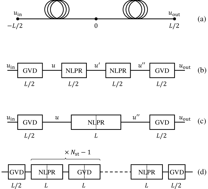
Figure 1: Derivation of the ESSFM model: (a) each propagation step of length $L$ is divided into two halves; (b) the approximated FRLP model is applied to each half (in reverse order in the second half); (c) the two adjacent NLPR blocks are combined into a single NLPR block; (d) the overall link of length $N_{\mathrm{st}}L$ is divided into $N_{\mathrm{st}}$ steps, each modelled as above, and pairs of adjacent GVD blocks are combined into single GVD blocks.

We approximate the propagation from $u_{\mathrm{in}}(t)\triangleq u(-L/2,t)$ to $u^{\prime}(t)\triangleq u(0,t)$ by applying an approximated version of the FRLP model [18, 5], which is derived in Appendix A and consists of a group-velocity dispersion (GVD) block followed by a nonlinear phase rotation (NLPR). On the other hand, using the same expedient employed in the symmetric version of the classical SSFM [20, Sec. 2.4.1], we approximate the propagation from $u^{\prime}(t)$ to $u_{\mathrm{out}}(t)\triangleq u(L/2,t)$ by applying the same model of the first half but in reverse order, obtaining the block diagram in Fig. 1(b). The cascade of the direct and reverse FRLP models ensures that error terms with an odd symmetry around $z=0$ cancel out, resulting in higher overall accuracy, and yields the symmetric configuration in Fig. 1(c), where the two half-length NLPR blocks are combined into a single NLPR block. After some calculation reported in Appendix A, we obtain the following model

$$u(t) =\int_{-\infty}^{+\infty}U_{\mathrm{in}}(f)H(L/2,f)e^{j2\pi ft}df$$ (2)

$$u^{\prime\prime}(t) =u(t)e^{-j\theta(t)}$$ (3)

$$u_{\mathrm{out}}(t) =\int_{-\infty}^{+\infty}U^{\prime\prime}(f)H(L/2,f)e^{j2\pi ft}df$$ (4)

where

$$H(z,f)=\exp\left(-j2\pi^{2}\beta_{2}f^{2}z\right)$$ (5)

is the transfer function due to the accumulated GVD after a propagation distance $z$;

$$\theta(t)=P\iint_{\mathbb{R}^{2}}K(\mu,\nu)U(\mu)U^{*}(\nu)e^{j2\pi(\mu-\nu)t}d\mu d\nu$$ (6)

is the NLPR due to Kerr nonlinearity (and its interaction with GVD); and

$$K(\mu,\nu)=\int_{-L/2}^{L/2}\gamma g(z)H(z,\mu)H^{*}(z,\nu)H(-z,\mu-\nu)dz$$ (7)

is a frequency-domain second-order Volterra kernel that accounts for the efficiency with which pairs of frequency components of the propagating signal contribute to the NLPR. A closed-form expression for (7) is given in Section II-D.

As in the classical SSFM, the propagation through a long link is usually handled by dividing it into $N_{\mathrm{st}}$ steps, where $N_{\mathrm{st}}$ is selected to obtain the desired tradeoff between complexity and accuracy. When modelling each step as in Fig. 1(c), pairs of adjacent half-length GVD blocks combine into single full-length GVD blocks, yielding the overall block diagram in Fig. 1(d).

For a practical implementation of the model for the development of DBP methods, which will be discussed in detail in Section III, it is convenient to consider a discrete-time representation of the signals. As shown in Appendix B, by assuming a sufficiently large sampling rate $R=1/T$, we obtain a discrete-time version of (6), in which the NLPR samples $\theta[k]\triangleq\theta(k/R)$ are related to the time-domain samples of the linearly propagated signal $u[k]\triangleq u(k/R)$ through a discrete-time second-order Volterra kernel. The corresponding expression is calculated in Appendix B and, as shown in (46), still involves the computation of an infinite number of terms. In practice, however, the discrete-time second-order Volterra kernel, whose coefficients $d[m,n]$ are defined in (47), has a limited duration that depends mainly on the GVD accumulated over the step length $L$ and (in minor part) on the pulse duration. This means that it can be practically truncated to a finite number of terms. Moreover, to further simplify the computation, we consider only the diagonal terms of the kernel, represented by the coefficients $c[m]\triangleq d[m,m]$ and neglect the (usually smaller) off-diagonal terms $d[m,n]$, with $m\neq n$. In this way, letting $N_{c}$ be the number of relevant pre- and post-cursor coefficients, (46) simplifies to

$$\theta[k]=\sum_{m=-N_{c}}^{N_{c}}c[m]|u[k-m]|^{2}$$ (8)

where

$$c[m]=\frac{P}{R^{2}}\int\limits_{-R/2}^{R/2}\int\limits_{-R/2}^{R/2}K(\mu,\nu)e^{j2\pi(\mu-\nu)m/R}d\mu d\nu$$ (9)

can be seen as the coefficients of the discrete-time impulse response that relates the signal intensity to the NLPR. Equations (2)–(4), (8), and (9) form the theoretical foundation for deriving the ESSFM and for analytically computing its coefficients. The necessary model extensions to derive the CC-ESSFM [11, 12] and the CB-ESSFM are detailed in the upcoming sections.

II-B Single-Polarization Multiband Signal

The accuracy of the ESSFM model in Fig. 1(d) depends on the amount of dispersion accumulated in each step, hence on the number of steps $N_{\mathrm{st}}$ in which the link is divided. The accumulated dispersion increases with the signal bandwidth, so that wider bandwidth signals typically requires more steps to achieve a prescribed accuracy. At the same time, more steps entails a higher computational complexity for DBP implementation, as detailed in Section III-D. Therefore, a possible solution to reduce computational complexity while maintaining high accuracy is to divide wide-band signals into subbands.

The calculations carried out for the single-band case can be readily extended to the multi-band scenario. In this context, the propagating signal $u(z,t)$, with bandwidth $B$, is partitioned into $N_{\mathrm{sb}}$ subbands and expressed as

$$u(z,t)=\sum_{i=1}^{N_{\mathrm{sb}}}u_{i}(z,t)$$ (10)

where $u_{i}(z,t)$ is the signal portion contained in the $i$th subband, centered at frequency $f_{i}$ and with a bandwidth $B/N_{\mathrm{sb}}$.

Since the impact of dispersion within each subband is significantly less pronounced than across the entire signal bandwidth, we can increase the step size $L$ of the model (thereby using fewer steps for the entire link) without sacrificing accuracy. At the same time, when dividing the signal into subbands, we need to decide how to handle the nonlinear interaction between them. The simplest option is to neglect it, applying the ESSFM separately to each subband as if it were the only propagating signal. In this way, we reduce the overall complexity (thanks to the increased step size), but we also lose accuracy (due to the neglected interband nonlinearity). An alternative option is to replace (10) in (1), hence expanding the nonlinear term in the latter into several sub-terms, typically categorized as self-phase modulation (SPM), cross-phase modulation (XPM), and four-wave mixing (FWM) terms [3]. Taking into account all sub-terms in the model would significantly amplify the complexity of each step, potentially nullifying the effort made to reduce it. However, the various terms have varying degrees of significance in contributing to the overall nonlinearity, particularly in the presence of dispersion. The strategy, therefore, is to discard less relevant terms, such as FWM ones, to strike the optimal balance between accuracy and complexity.

By replacing (10) in (1), and neglecting (non-degenerate) FWM terms, we obtain a set of $N_{\text{sb}}$ coupled NLSEs

$$\begin{gathered}\frac{\partial u_{i}}{\partial z}=j\frac{\beta_{2}}{2}\frac{\partial^{2}u_{i}}{\partial t^{2}}-j\gamma Pg(z)\biggl{(}|u_{i}|^{2}+2\sum_{\ell\neq i}|u_{\ell}|^{2}\biggr{)}u_{i}\\ i=1,\ldots,N_{\mathrm{sb}}\end{gathered}$$ (11)

each including an SPM term and $N_{\mathrm{sb}}-1$ XPM terms.

As in the single-channel case, we approximate the propagation through the step of length $L$ depicted in Fig. 1(a) by using the FRLP model in a split-step symmetric configuration, including this time also the XPM terms in the NLPR [5, eq. (9)]. The solution for the signal $u_{i}$ in the $i$th subband, whose derivation is omitted due to its similarity with the single-band case, can still be expressed as in (2)–(4) and visualized by the block diagram in Fig. 1(c) (adding the subscript $i$ to all involved signals), but with a different NLPR that includes both SPM and XPM terms

$$\theta_{i}(t) =P\biggl{(}\iint_{\mathbb{R}^{2}}K(\mu,\nu)U_{i}(\mu)U_{i}^{*}(\nu)e^{2\pi j(\mu-\nu)t}d\mu d\nu$$

$$\quad+\sum_{\ell\neq i}\iint_{\mathbb{R}^{2}}2K(\mu,\nu)U_{\ell}(\mu)U_{\ell}^{*}(\nu)e^{2\pi j(\mu-\nu)t}d\mu d\nu\biggr{)}$$ (12)

Considering a discrete-time representation of the signals; letting $u_{i}[k]\triangleq u_{i}(k/R^{\prime})$ and $\theta_{i}[k]\triangleq\theta_{i}(k/R^{\prime})$ be the samples of the signal and NLPR, respectively, taken at rate $R^{\prime}=R/N_{\mathrm{sb}}$; truncating the discrete-time Volterra kernel; and neglecting its off-diagonal terms as in the single-band case, we eventually obtain

$$\theta_{i}[k] =\sum_{m=-N_{c}}^{N_{c}}c_{ii}[m]|u_{\ell}[k-m]|^{2}$$

$$\quad+2\sum_{\ell\neq i}\sum_{m=-N_{c}}^{N_{c}}c_{i\ell}[m]|u_{\ell}[k-m]|^{2}$$ (13)

where

$$c_{i\ell}[m]=\frac{P}{R^{\prime 2}}\int\limits_{f_{i\ell}-R^{\prime}/2}^{f_{i\ell}+R^{\prime}/2}\int\limits_{f_{i\ell}-R^{\prime}/2}^{f_{i\ell}+R^{\prime}/2}K(\mu,\nu)e^{j2\pi(\mu-\nu)m/R^{\prime}}d\mu d\nu$$ (14)

is the $m$-th coefficient of the impulse response that accounts for the impact of the intensity of the $\ell$th subband on the NLPR of the $i$th subband, and $f_{i\ell}=f_{\ell}-f_{i}$ is the frequency separation between the two subbands. For $i=\ell$, $f_{i\ell}=0$ and (14) reduces to (9).For a larger frequency separation $f_{i\ell}$, the walk-off between subbands induced by dispersion increases. Numerically, this effect results in a more compact kernel $K(\mu,\nu)$ in frequency domain and, in turn, in a slower decay of the magnitude of the coefficients $c_{i\ell}[m]$ with $m$, i.e., in a wider impulse response of the filter. This implies that, in general, the impulse response can be truncated to a number of coefficients $N_{c}$ that depends on $\ell-i$, though we omitted this dependence in (13) to keep the notation simple. For the same reason, the NLPR generated by distant (with large $f_{i\ell})$ subbands varies slowly with time, meaning that its effect is more easily compensated for by the carrier phase recovery algorithm and can be neglected when using the ESSFM algorithm for DBP.

II-C Dual-Polarization Multiband System

The previous model can be eventually extended to the case of a dual-polarization signal, whose propagation is governed by the Manakov equation [21]—formally equal to (1) but considering $u=(x,y)$ as the Jones vector collecting the normalized complex envelopes of the two polarization components, $x$ and $y$, and $|u|^{2}=|x|^{2}+|y|^{2}$ as the squared-norm of the vector. As in (10), we divide the signal into $N_{\mathrm{sb}}$ subbands, where each subband contains two polarization components $u_{i}=(x_{i},y_{i})$, and replace them in (1). In this case, besides SPM, XPM, and FWM, we obtain also cross-polarization modulation (XPolM) terms [22]. Though XPolM can typically be as relevant as XPM, its effect cannot be simply represented as an NLPR, and its inclusion in the model significantly increases the complexity. In this case, we consider two possible solutions to obtain a good trade-off between accuracy and complexity. The first solution is obtained by omitting both FWM and XPolM terms, obtaining a set of $N_{\text{sb}}$ coupled Manakov equations

$$\begin{gathered}\frac{\partial u_{i}}{\partial z}=j\frac{\beta_{2}}{2}\frac{\partial^{2}u_{i}}{\partial t^{2}}-j\gamma Pg(z)\left(|u_{i}|^{2}+\frac{3}{2}\sum_{\ell\neq i}|u_{\ell}|^{2}\right)u_{i}\\ i=1,\ldots,N_{\mathrm{sb}}\end{gathered}$$ (15)

formally equivalent to (11) but for the 3/2 degeneracy factor in front of the XPM terms (instead of 2) and for the vector interpretation as explained above. Consequently, the propagation of the $i$th subband over the step of length $L$ depicted in Fig. 1(a) can still be expressed as in (2)–(4) and visualized by the block diagram in Fig. 1(c), provided that the signals are interpreted as two-component vectors, and the GVD and NLPR are applied to each polarization component. In this case, considering a discrete-time representation of the signals, the NLPR in the $i$th subband can be expressed as

$$\theta_{i}[k] =\sum_{m=-N_{c}}^{N_{c}}c_{ii}[m]|u_{i}[k-m]|^{2}$$

$$\quad+\frac{3}{2}\sum_{\ell\neq i}\sum_{m=-N_{c}}^{N_{c}}c_{i\ell}[m]|u_{\ell}[k-m]|^{2}$$ (16)

i.e., as in the single-polarization case (13), but with the squared norm replacing the squared modulus, and a 3/2 degeneracy factor in front of the XPM terms. The coefficients are the same as in (14). This solution allows to describe the reduced complexity CC-ESSFM in [12] and will be used for the development of the CB-ESSFM in III-A.

On the other hand, the second solution is obtained by neglecting FWM terms and incorporating only certain XPolM terms in the multi-band expansion of the vector form of (1). Specifically, to avoid a significant increase in computational complexity, we include only those terms that can still be expressed as an NLPR, albeit of a different entity for the two polarizations. In this case, it is necessary to represent the evolution of the two polarization components of each subband with two coupled equations, obtaining a set of $2N_{\mathrm{sb}}$ coupled differential equations [23]

$$\frac{\partial x_{i}}{\partial z} =j\beta_{2}\frac{\partial^{2}x_{i}}{\partial t^{2}}-j\gamma Pg(z)$$

$$\quad+\biggl{(}|x_{i}|^{2}+|y_{i}|^{2}+\sum_{\ell\neq i}2|x_{\ell}|^{2}+|y_{\ell}|^{2}\biggr{)}x_{i}$$ (17)

$$\frac{\partial y_{i}}{\partial z} =j\beta_{2}\frac{\partial^{2}y_{i}}{\partial t^{2}}-j\gamma Pg(z)$$

$$\quad+\biggl{(}|x_{i}|^{2}+|y_{i}|^{2}+\sum_{\ell\neq i}|x_{\ell}|^{2}+2|y_{\ell}|^{2}\biggr{)}y_{i}$$ (18)

$$i=1,\ldots,N_{\mathrm{sb}}$$

The equations above imply that the XPM induced by co-polarized subbands is twice as effective as the XPM resulting from orthogonally-polarized subbands. This stands in contrast to the simpler model in (15), where the same XPM affects both polarizations, corresponding to the average XPM affecting the two polarizations in (17) and (18). For the rest, the equations are similar to those in (11), and the application of the FRLP method, whose development is omitted due to its similarity with the previous cases, yields a similar model. The propagation of the $i$th subband over the step of length $L$ depicted in Fig. 1(a) can still be expressed as in (2)–(4), but replacing the NLPR in (3) with different NLPRs $\theta_{i}^{x}(t)$ and $\theta_{i}^{y}(t)$ for the two polarization components

$$x_{i}^{\prime\prime}(t) =x_{i}(t)\exp\bigl{(}j\theta_{i}^{x}(t)\bigr{)}$$ (19)

$$y_{i}^{\prime\prime}(t) =y_{i}(t)\exp\bigl{(}j\theta_{i}^{y}(t)\bigr{)}$$ (20)

Eventually, considering a discrete-time representation of the signals and letting $x_{i}[k]=x_{i}(k/R^{\prime})$, $y_{i}[k]=y_{i}(k/R^{\prime})$, $\theta_{i}^{x}[k]=\theta_{i}^{x}(k/R^{\prime})$, and $\theta_{i}^{y}[k]=\theta_{i}^{y}(k/R^{\prime})$, the NLPRs can be expressed as

$$\theta_{i}^{x}[k] =\sum_{m=-N_{c}}^{N_{c}}c_{ii}[m]\bigl{(}x_{i}^{2}[k+m]+y_{i}^{2}[k+m]\bigr{)}$$

$$\quad+\sum_{\ell\neq i}\sum_{m=-N_{c}}^{N_{c}}c_{i\ell}[m]\bigl{(}2x_{\ell}^{2}[k+m]+y_{\ell}^{2}[k+m]\bigr{)}\!$$ (21)

$$\theta_{i}^{y}[k] =\sum_{m=-N_{c}}^{N_{c}}c_{ii}[m]\bigl{(}x_{i}^{2}[k+m]+y_{i}^{2}[k+m]\bigr{)}$$

$$\quad+\sum_{\ell\neq i}\sum_{m=-N_{c}}^{N_{c}}c_{i\ell}[m]\bigl{(}x_{\ell}^{2}[k+m]+2y_{\ell}^{2}[k+m]\bigr{)}$$ (22)

The coefficients $c_{i\ell}[m]$ are as in (14) and do not depend on the particular polarization. This solution allows to describe the full-complexity CC-ESSFM [11, 12] and may be used also for the CB-ESSFM, though not done in this paper.

II-D Evaluation of the CB-ESSFM Coefficients

In this Section, we provide an analytical expression for the kernel function (7) and a numerical procedure for the evaluation of the CB-ESSFM coefficients defined in (14). For simplicity, we assume that the step in Fig. 1(a) consists of $N_{\text{sp}}$ identical spans of fiber of length $L/N_{\text{sp}}$, with attenuation coefficient $\alpha,$ dispersion parameter $\beta_{2}$, nonlinear coefficient $\gamma$, and periodic amplification at the end of each span which exactly compensates for the span loss. In this case, letting $a=\alpha/2$ and $b\triangleq 2\pi^{2}\beta_{2}\nu(\mu-\nu)$, after a few calculations reported in Appendix C, the kernel function can be expressed as

$$K(\mu,\nu)=\gamma e^{-aL/N_{\mathrm{sp}}}\frac{\sinh\bigl{(}(a+jb)L/N_{\mathrm{sp}}\bigr{)}\sin(bL)}{(a+jb)\sin(bL/N_{\mathrm{sp}})}$$ (23)

The expression (23) can be used also when the step is just a fraction of a span. In this case, it is sufficient to set $N_{\mathrm{sp}}=1$, $L$ to the actual length of the step (not the whole span), and the reference power $P$ in (14) to the power at the input of the step. For instance, if a span of length $L_{\mathrm{sp}}$ is divided into three equal steps, the kernel function is the same for all the steps and is obtained by setting $L=L_{\mathrm{sp}}/3$ in (23), while the power $P$ to be used in (14) is different: it equals the launch power in the first step, is attenuated by $\exp(-\alpha L)$ in the second step, and by $\exp(-2\alpha L)$ in the third step. The approach can easily be extended to derive more general closed-form expressions for steps that include several pieces of fiber with different length and propagation parameters.

Given the kernel function (23), the coefficients $c_{i\ell}[m]$ can be evaluated numerically from (14), e.g., as the diagonal terms of the two-dimensional FFT of the kernel function (23), evaluated over a grid of $(2N_{c}+1)\times(2N_{c}+1)$ frequency values in the range $\mu,\nu\in[f_{i\ell}-R^{\prime}/2,f_{i\ell}+R^{\prime}/2]$. Alternatively, as discussed in Section III, the CB-ESSFM coefficients can also be obtained through a numerical optimization procedure aimed at minimizing/maximizing some loss/performance metric (e.g., the mean square error).

Here we report some general properties of the coefficients $c_{i\ell}[m]$, which can be inferred from (14) and (23) and can be used to simplify their evaluation and optimization, as discussed in greater detail in Section III:

• they are linearly proportional to the product $\gamma P$;

• they are independent of the modulation format (e.g., they are the same for 16-QAM and 64-QAM, with and without shaping);

• they depend on the frequency distance $f_{\ell}-f_{i}$ between the interfering channel and the observed channel, not on their absolute position, meaning that, for equally spaced channels, they depend on $i$ and $\ell$ only through the difference $\ell-i$, so that

  $$c_{i,\ell}[m]=c_{i+k,\ell+k}[m],\quad\forall k\in\mathbb{Z}$$ (24)

• they satisfy the symmetry condition

  $$c_{i,\ell}[m]=c_{\ell,i}[-m]$$ (25)

  implying that the SPM coefficients have always an even symmetry

  $$c_{i,i}[m]=c_{i,i}[-m].$$ (26)

III Implementation

This Section discusses the practical implementation of the proposed DBP method and is divided into four parts. The first part describes the signal processing algorithm. The second part explains the procedure for the numerical optimization of the CB-ESSFM coefficients; the third part introduces an alternative implementation based on asymmetric steps and discusses the optimization of their splitting ratio. Finally, the last part provides information about the computational complexity of the method.

III-A The Coupled-Band ESSFM (CB-ESSFM)

The proposed DBP algorithm is based on the theoretical model described in the previous section and on the overlap-and-save technique [24], as schematically depicted in Fig. 2. First, the received signal is sampled at $n$ samples per symbol, where the oversampling factor $n\geq 1+r$ is selected to account for the roll-off factor $r$ of the modulation pulses and the bandwidth expansion induced by nonlinearity.

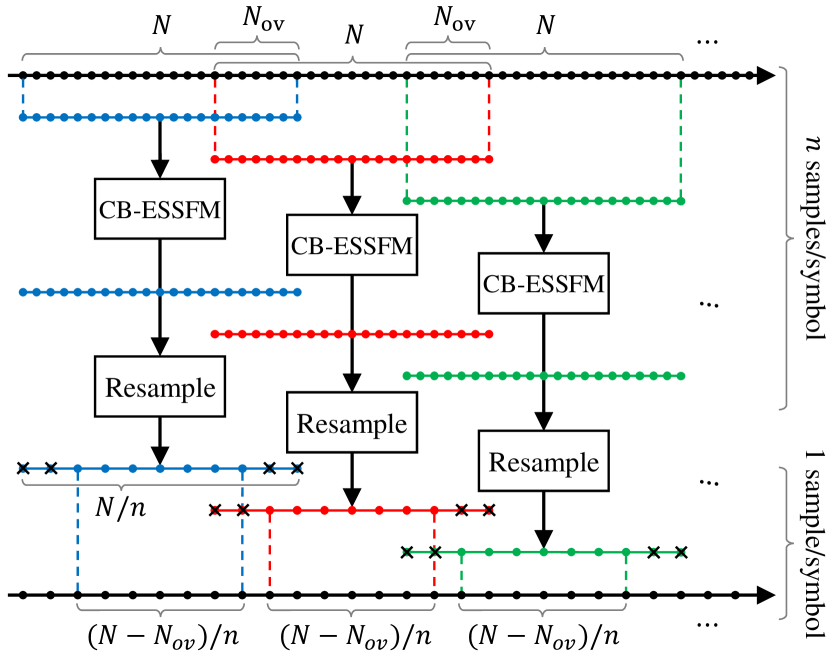
Figure 2: The received signal is processed by the CB-ESSFM algorithm by using oversampling and overlap and save.

The sequence of 4D samples (two polarizations and two quadratures per sample) is then processed block-wise by using the overlap-and-save technique [24]. In practice, the sequence is divided into partially overlapping blocks of $N$ samples, with an overlap of $N_{\mathrm{ov}}$ samples. The overlap should at least equal the duration of the overall channel response, which is mainly determined by the accumulated GVD. Each block is processed by the CB-ESSFM algorithm, obtaining the corresponding $N$ output samples, and then resampled at one sample per symbol, obtaining $N/n$ samples. Eventually, the overlapping samples are discarded—$N_{\mathrm{ov}}/2n$ on each side of each block—while the remaining $(N-N_{\mathrm{ov}})/n$ per block are saved and recombined to form the whole output sequence.

The processing performed by the CB-ESSFM algorithm on each block of $N$ 4D samples follows the scheme in Fig. 1(d), with the dual-polarization multiband processing described in Section II-C and the NLPR in (16). The algorithm is further detailed in Fig. 3 and 4.

Figure 3: CB-ESSFM algorithm with $N_{\mathrm{st}}$ steps and $N_{\mathrm{sb}}$ subbands.

At the input, two complex FFTs (CFFTs)—one for each polarization—are performed on the whole block of $N$ samples, followed by a demultiplexer (DEMUX) that divides the signal into $N_{\mathrm{sb}}$ subbands (at no cost in the frequency domain), each represented by $N^{\prime}=N/N_{\mathrm{sb}}$ samples. Then, GVD compensation and nonlinear phase rotation (NLPR) are iteratively performed $N_{\mathrm{st}}$ times, each followed, respectively, by $2N_{\mathrm{sb}}$ (one per each subband and polarization) inverse and direct CFFTs of size $N^{\prime}$ to perform GVD compensation in the frequency domain and nonlinear phase rotation in the time domain. Finally, one additional GVD compensation is performed, followed by a multiplexer (MUX) that recombines the subbands and two inverse CFFTs of size $N$.

The GVD compensation block consists in the multiplication of both polarizations of each signal component (at frequency $f_{k}$) by the corresponding value of the fiber transfer function $h_{k}=\exp(j2\pi^{2}\beta_{2}\Delta zf_{k}^{2})$, where $\Delta z$ is the fiber length for which GVD compensation is applied. In the configuration shown in Fig. 1(d), the link is divided into $N_{\mathrm{st}}$ steps of length $L$, and each step is symmetrically split into two halves of length $L/2$, so that $\Delta z=L/2$ in the first and last GVD compensation blocks, while $\Delta z=L$ in all the others. If necessary, the method could be easily adjusted to accommodate a variable step size and a different splitting ratio, with no significant changes to the implementation scheme and complexity. The benefits of an asymmetric configuration with an optimized splitting ratio are discussed in Section III-C.

The NLPR block follows the process shown in Fig. 4.

Figure 4: Nonlinear phase rotation (NLPR) of the CB-ESSFM algorithm with $N_{\mathrm{sb}}$ subbands.

First, the intensity (squared norm) of the $N^{\prime}$ 4D samples on each subband is computed. Then, MIMO filtering of the $N_{\mathrm{sb}}$ real intensity signals is implemented in frequency domain to compute the $N_{\mathrm{sb}}$ NLPRs. This operation, described in (16) in the time domain, is equivalently but more efficiently implemented in the frequency domain by performing $N_{\mathrm{sb}}$ RFFT of size $N^{\prime}$, multiplying the resulting vector of $N_{\mathrm{sb}}$ samples at each frequency component by the corresponding $N_{\mathrm{sb}}\times N_{\mathrm{sb}}$ MIMO transfer matrix, and then performing $N_{\mathrm{sb}}$ inverse RFFTs of size $N^{\prime}$ to go back to the time domain. The MIMO transfer matrix is obtained offline by transforming (through FFT) the MIMO impulse response matrix, whose elements correspond to the CB-ESSFM coefficients in (14). Finally, each 4D output sample is obtained by multiplying each polarization component by the corresponding complex-exponential term (the same for both polarizations).

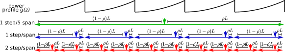
Figure 5: Attenuation profile (in the backpropagation configuration) with different SSFM configurations.

III-B Optimization of the CB-ESSFM Coefficients

The CB-ESSFM coefficients (or their FFT) needed for implementing the MIMO filter in Fig. 4 can be obtained analytically as explained in Section II-D, with minor modifications required to account for non-uniform span lengths or asymmetric splitting ratios.

Alternatively, they can also be found by numerical (offline) optimization, in order to maximize the system performance and/or consider unknown or complex system configurations. In the remainder of the paper, unless otherwise stated, we will use the latter approach, selecting the coefficients that minimize the mean square error between the transmitted and received symbols. To reduce the complexity of the optimization (which is, however, done offline and does not affect the complexity of the DSP) we

• assume that the coefficients are the same in each step, but for rescaling them proportionally to the signal power at the input of each step when more than one step per span is used;

• assume the symmetries in (24)–(26);

• consider a finite number of coefficients, which depends on the channel memory: the number of coefficients for the interaction of the subbands $\ell$ and $\ell+h$ is $2N_{c}(h)+1\approx\pi L\beta_{2}(nR/N_{\text{sb}})^{2}(h+1)$.

Given the above assumptions, letting $\mathbf{c}_{h}$ be the vector that collects the $2N_{c}(h)+1$ coefficients that determine the interaction between subbands $\ell$ and $\ell+h$ (the same for any $\ell$), the optimization problem consists in finding the vectors $\mathbf{c}_{0},\mathbf{c}_{1},\ldots,\mathbf{c}_{N_{\mathrm{sb}}-1}$ that minimize the mean square error between the received symbols (after DBP, matched filtering, resampling, and mean phase rotation removal) and the transmitted symbols. To simplify the problem, we optimize the $N_{\mathrm{sb}}$ vectors separately, in $N_{\mathrm{sb}}$ iterations: in the $i$th iteration, we optimize $\mathbf{c}_{i-1}$, keeping $\mathbf{c}_{0},\ldots,\mathbf{c}_{i-2}$ fixed at the values obtained at the previous iterations, and setting $\mathbf{c}_{i},\ldots,\mathbf{c}_{N_{\mathrm{sb}}-1-2}$ to zero. The optimization of $\mathbf{c}_{i-1}$ is performed by using Matlab’s solver for nonlinear least squares problems based on the trust-region-reflective algorithm. In our simulations, we did not observe substantial convergence issues nor a critical dependence of the solution on the initial values, which were simply set to the values corresponding to a standard SSFM (all zeros, but for the central coefficient of $\mathbf{c}_{0}$ equal to the average nonlinear phase rotation over the step).

The assumptions made above could be relaxed to improve the performance of the DBP algorithm. For instance, one could use a different set of CB-ESSFM coefficients in each nonlinear step. However, this change may lead to a more complex training phase. This possibility has not been investigated in this work and is left for future study..

III-C Optimization of the splitting ratio

In the symmetric configuration shown in Fig. 1(a)–(d), the NLPR is positioned in the middle of the step, sandwiched between two equal GVD steps of length $L/2$. For a short piece of fiber with negligible attenuation, this configuration ensures high accuracy thanks to the cancellation of error terms with an odd symmetry around $z=0$. This happens if the amount of nonlinearity and dispersion accumulated in the two half steps is comparable. However, the ESSFM is designed to reduce the number of propagation steps compared to the SSFM, with each step possibly encompassing one or more fiber spans, so that the power profile $g(z)$ (hence the accumulated nonlinearity) may be highly asymmetric with respect to the middle of the step. In this situation, an asymmetric configuration that divides the span in two portions with comparable accumulated nonlinearity is expected to yield better results.

Therefore, we consider the more general configuration illustrated in Fig. 5(a), in which the NLPR is preceded by a GVD block of length $(1-\rho)L$ and followed by a GVD block of length $\rho L$, where $\rho$ is referred to as splitting ratio. As an example, Fig.5(b) shows the power profile $g(z)$ in a five-span (backward) link and, below, three different DBP configurations: a single step for the whole link; one step per span; and two steps per span. The vertical arrows indicate the NLPR position within each step. With a single step, a balanced division of nonlinear effects is approximately obtained with a symmetric configuration ($\rho=0.5$)—the approximation becoming more accurate for a higher number of spans. For instance, a symmetric configuration was shown to be optimal for the single-step DBP algorithm employed in [8]. On the other hand, with one step per span, nonlinear effects take place mostly in the last portion of each step, so that an asymmetric configuration with $\rho<0.5$ results in a more balanced distribution of nonlinear effects in the two portions of the step. Finally, with two steps per span, a balanced distribution is still obtained with splitting ratio $\rho<0.5$, but higher (approximately doubled) than in the previous case. Further increasing the number of steps makes the attenuation in each step less and less relevant, requiring the optimal $\rho$ to approach again the symmetric configuration (as typically done in the conventional SSFM). These heuristic considerations will be verified numerically in Section IV-C.

With asymmetric steps, the overall DBP implementation changes only slightly with respect to the symmetric case shown in Fig. 1(d). In fact, couple of GVD blocks from adjacent steps can still be combined to form a single GVD block of length $L$, and only the length of the first and last GVD blocks must be modified to $(1-\rho)L$ and $\rho L$, respectively.

III-D Complexity

The computational complexity of the algorithm is assessed based on by the number of real multiplications (RMs) and real additions (RAs) required for each 2D symbol. In our analysis, we assume that each complex addition is carried out with two RAs, while each complex multiplication (CM) requires three RMs and five RAs [25]. If one of the multipliers of a CM is known in advance, only three out of the five RAs need to be computed in real-time, as two of them can be precomputed offline. Analogously, if a couple of CMs involve the same complex multiplier, two RAs can be computed only once and used for both the CMs, so that each CM requires, on average, three RMs and four RAs. Finally, if one of the multipliers is real, the CM reduces to just two RMs. Moreover, we assume that the CFFT of $N$ complex samples is implemented by the split-radix algorithm [26], which requires $N\log_{2}N-3N+4$ RMs and $3N\log_{2}N-3N+4$ RAs, and that the RFFT requires approximately half the RMs and RAs of the CFFT [26].

At the output of the CB-ESSFM, each 4D output sample corresponds to a couple of 2D symbols—one per polarization. Thus, the overall computational complexity, is given by the following equations

$$C_{M} =\frac{n\cdot N_{\mathrm{RM}}(N,N_{\mathrm{st}},N_{\mathrm{sb}})}{2\cdot(N-N_{\mathrm{ov}})}$$ RM/2D symb. (27)

$$C_{A} =\frac{n\cdot N_{\mathrm{RA}}(N,N_{\mathrm{st}},N_{\mathrm{sb}})}{2\cdot(N-N_{\mathrm{ov}})}$$ RA/2D symb. (28)

where $N_{\mathrm{RM}}$ and $N_{\mathrm{RA}}$ denote, respectively, the number of RMs and RAs required by the CB-ESSFM to process a block of $N$ 4D samples, and we have made explicit their dependence on $N$ and on the number of steps $N_{\mathrm{st}}$ and of subbands $N_{\mathrm{sb}}$ employed by the algorithm.

The expression for $N_{\mathrm{RM}}$ and $N_{\mathrm{RA}}$ is derived here. The CB-ESSFM in Fig. 3 applied to a block of $N$ samples, with $N_{\text{sb}}$ bands, and $N_{\text{st}}$ steps uses $4$ (direct or inverse) CFFTs of size $N$, $4N_{\mathrm{sb}}N_{\mathrm{st}}$ CFFTs of size $N^{\prime}=N/N_{\mathrm{sb}}$, $N_{\mathrm{st}}+1$ GVD compensations, and $N_{\mathrm{st}}$ NLPRs. Concerning GVD compensation, it requires only $2N$ CMs—two per each polarization of each 4D sample—with a reduced complexity due to the fixed multiplier, and because the factor $h_{k}$ is fixed and can be precomputed offline. This corresponds to $6N$ RMs and $6N$ RAs for each GVD compensation step.

Regarding the cost of each NLPR, the computation of the intensity of the $N^{\prime}$ 4D samples uses $4N$ RMs and $3N$ RAs. For what concerns the MIMO filtering, by exploiting the Hermitian symmetry of the $N^{\prime}$ frequency components (both the signal intensity and the CB-ESSFM coefficients are real in time domain), only half ($N^{\prime}/2$) matrix–vector multiplications need to be actually implemented. Considering that the elements of the MIMO transfer matrix can be precomputed offline, and that the diagonal elements are real due to the even symmetry of the SPM coefficients in (26), each matrix–vector multiplication requires $N_{\mathrm{sb}}(N_{\mathrm{sb}}-1)$ CMs with one fixed multiplier, $N_{\mathrm{sb}}$ CMs with one real multiplier, and $N_{\mathrm{sb}}(N_{\mathrm{sb}}-1)$ complex additions. Overall, MIMO filtering requires

$$N\log_{2}N^{\prime}+\frac{N}{2}(3N_{\mathrm{sb}}-7)+4N_{\mathrm{sb}} \mathrm{RM}$$

$$3N\log_{2}N^{\prime}+\frac{N}{2}(5N_{\mathrm{sb}}-11)+4N_{\mathrm{sb}} \mathrm{RA}$$

For the computation of the complex exponential terms, we assume a look-up-table implementation or similar approach, so we neglect its complexity. The multiplication by the complex-exponential term requires a couple of CMs with a common multiplier, resulting in $6N$ RMs and $8N$ RAs to obtain the $N$ 4D samples ($N^{\prime}$ on each subband). Overall, by combining the cost of intensity computation, MIMO filtering, and output CMs, the NLPR step in Fig. 4 requires

$$N\log_{2}N^{\prime}+\frac{N}{2}(3N_{\mathrm{sb}}+13)+4N_{\mathrm{sb}} \mathrm{RM}$$

$$3N\log_{2}N^{\prime}+\frac{N}{2}(5N_{\mathrm{sb}}+11)+4N_{\mathrm{sb}} \mathrm{RA}$$

In total, adding up the number of RMs and RAs required by all the steps of the CB-ESSFM algorithm in Fig. 2, and replacing them in (27) and (28), we obtain the following equations for the computational complexity 9

$$C_{\mathrm{RM}} =\frac{n}{2}\frac{N}{N-N_{\mathrm{ov}}}\left((5N_{\mathrm{st}}+4)\log_{2}\frac{N}{N_{\mathrm{sb}}}+N_{\mathrm{st}}\frac{3N_{\mathrm{sb}}+1}{2}\right.$$

$$\left.{}+4\log_{2}N_{\mathrm{sb}}-6+\frac{20N_{\mathrm{sb}}N_{\mathrm{st}}+16}{N}\right)\quad\mathrm{RM/2D\,symb.}$$ (29)

$$C_{\mathrm{RA}} =\frac{n}{2}\frac{N}{N-N_{\mathrm{ov}}}\left((15N_{\mathrm{st}}+12)\log_{2}\frac{N}{N_{\mathrm{sb}}}+N_{\mathrm{st}}\frac{5N_{\mathrm{sb}}-1}{2}\right.$$

$$\left.{}+12\log_{2}N_{\mathrm{sb}}-6+\frac{20N_{\mathrm{sb}}N_{\mathrm{st}}+16}{N}\right)\quad\mathrm{RA/2D\,symb.}$$ (30)

For the sake of comparison, we report below the complexity of the other DBP methods discussed in this work. The (single-band) ESSFM can be obtained simply by considering a CB-ESSFM with a single band (frequency-domain NLPR), or can be alternatively implemented with a time-domain NLPR, with a complexity that depends on the number of real symmetric CB-ESSFM coefficients $2N_{c}+1$ as

$$C_{\mathrm{RM}} =\frac{n}{2}\frac{N}{N-N_{\mathrm{ov}}}\left((N_{\mathrm{st}}+1)\left(4\log_{2}N-6+\frac{16}{N}\right)\right.$$

$$\left.{}+N_{\mathrm{st}}(11+N_{c})\right)\quad\mathrm{RM/2D\,symb.}$$ (31)

$$C_{\mathrm{RA}} =\frac{n}{2}\frac{N}{N-N_{\mathrm{ov}}}\left((N_{\mathrm{st}}+1)\left(12\log_{2}N-6+\frac{16}{N}\right)\right.$$

$$\left.{}+N_{\mathrm{st}}(11+2N_{c})\right)\quad\mathrm{RA/2D\,symb.}$$ (32)

The complexity of the SSFM and OSSFM is obtained by setting $N_{c}=0$ in (31) and (32), while the complexity of GVD compensation is obtained by setting $N_{\mathrm{st}}=0$.

IV Numerical results

IV-A System Description

The link consists of $15$ (unless otherwise stated) spans of $80$ km single-mode fiber (SMF), with attenuation $\alpha_{\text{dB}}=0.2\,\mathrm{dB/km}$, dispersion $D=17\thinspace\text{ps}/\text{nm}/\text{km}$, and Kerr parameter $\gamma=1.27\thinspace\text{W}^{-1}\text{km}^{-1}$. After each span, an erbium-doped fiber amplifier (EDFA) with a noise figure of $4.5$ dB compensates for the span loss. The transmitted signal is made of five identical wavelength division multiplexed (WDM) channels with $100$ GHz spacing. Each channel carries a uniform dual-polarization 64-QAM signal, with baud rate $R=93$ GBd and (frequency-domain) root-raised-cosine pulses with rolloff $r=0.05$. At the receiver side, the central channel is demultiplexed and processed by either electronic dispersion compensation (EDC) or digital backpropagation (DBP) with different possible algorithms: the CB-ESSFM described in this paper; the ESSFM proposed in [9, 10], equivalent to CB-ESSFM with $N_{\mathrm{sb}}=1$ and $\rho=0.5$; the optimized SSFM (OSSFM), corresponding to a standard SSFM with optimized nonlinear coefficient and equivalent to an ESSFM with a single coefficient ($N_{c}=0$); and ideal DBP, practically obtained from a standard SSFM with a very large number of steps $N_{\mathrm{st}}$, sufficient to achieve performance saturation. Unless otherwise stated, all DBP algorithms use $n=1.125$ samples/symbol. Next, the signal undergoes matched filtering, resampling at 1 sample/symbol, and mean phase rotation removal. Finally, the performance is evaluated in terms of received signal-to-noise ratio (SNR), where noise is defined as the difference between the output samples and the transmitted symbols. The results shown in the following are all obtained at the optimal launch power (approximately between $3$ and $4$ dBm per channel).

The gains shown in the following are expected to be maintained even with different modulation formats (even using constellation shaping) and including carrier phase recovery, since they are effective in reducing inter-channel nonlinearity, while the CB-ESSFM compensates for intra-channel nonlinearities [28].

IV-B CB-ESSFM Coefficients: Analytical Evaluation vs Numerical Optimization

Figures 6(a)-(b) compare the CB-ESSFM coefficients obtained analytically as explained in Section II-D with those obtained by the numerical optimization procedure described in Section III-B. The coefficents are evaluated for the $15\times 80$ km link, considering $N_{\text{st}}=5$ identical DBP steps (each made of three fiber spans) and $N_{\text{sb}}=2$ bands, and their values are normalized to the average nonlinear phase rotation over the step. Fig. 6(a) shows the intraband coefficients $c_{11}[m]$, while Fig. 6(b) shows the interband coefficients $c_{12}[m]$. Both figures show that the two approaches yield similar values, confirming the accuracy of the theoretical model developed in Section II and the possibility of using the analytical procedure to configure the algorithm coefficients or to initialize them in the numerical optimization. . In the next sections, we will always use the coefficients obtained by numerical optimization.

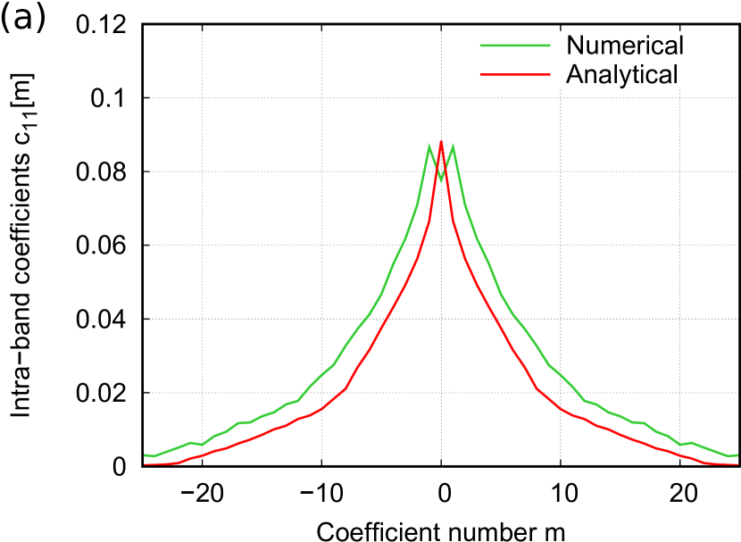
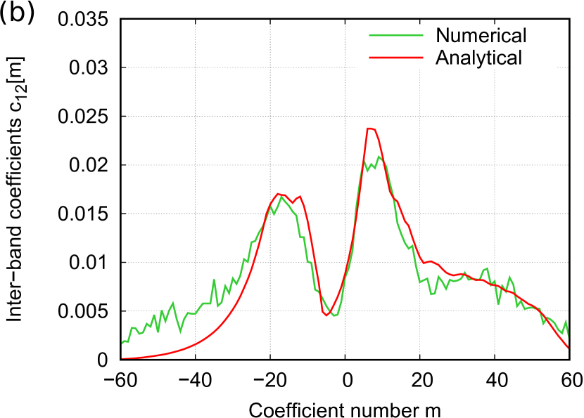
Figure 6: Comparison of CB-ESSFM coefficients obtained analytically or by numerical optimization for the case of $N_{\text{st}}=5$ steps: (a) intra-band coefficients $c_{11}[m]$; (b) inter-band coefficients $c_{12}[m]$.

IV-C System Performance

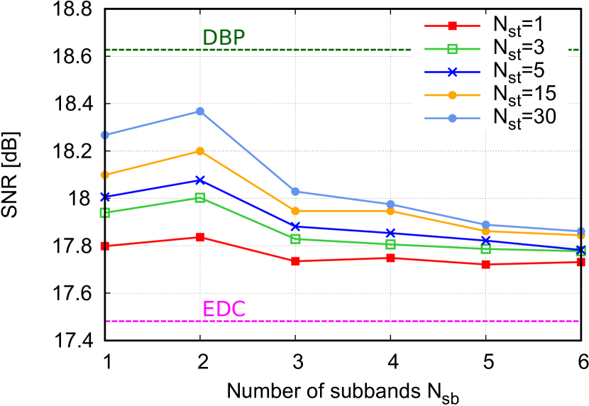
Figure 7: SNR versus number of subbands $N_{\text{sb}}$ with CB-ESSFM for different $N_{\text{st}}$ values. $\rho=0.5$, $n=1.125$.

We start by investigating how the division in subbands and the optimization of the splitting ratio affect the performance of the proposed algorithm. Fig. 7 shows the SNR obtained with the symmetric CB-ESSFM ($\rho=0.5$) as a functionof the number of subbands $N_{\text{sb}}$ for different numbers of steps $N_{\text{st}}$. . As a reference, the performance of EDC and ideal DBP are also shown. As expected, the SNR improves when $N_{\text{st}}$ increases. On the other hand, as discussed in Section II-B, increasing $N_{\mathrm{sb}}$ causes two opposite effects: the reduction of dispersion within each subband, which improves model accuracy; and the appearance of additional interband nonlinear interactions not included in the model (FWM and XPolM), which degrades accuracy. Regardless of the number of steps, the best tradeoff between the two effects is obtained with $N_{\text{sb}}=2$ subbands, , with a gain of $0.1$ dB with respect to the single-band case for $N_{\text{st}}=15$, and a total gain of $0.72\,\mathrm{dB}$ with respect to EDC.

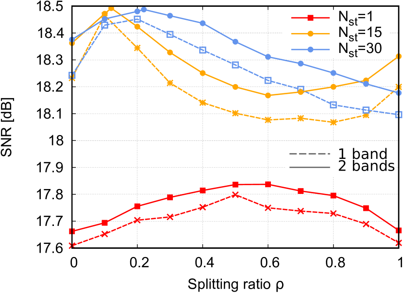
Figure 8: SNR versus splitting ratio $\rho$ with CB-ESSFM with $N_{\text{sb}}=1$ band (dashed) and $N_{\text{sb}}=2$ bands (solid). $n=1.125$

Next, Fig. 8 shows the SNR as a function of the splitting ratio $\rho$ for different numbers of steps $N_{\mathrm{st}}$ and considering either a single band or two subbands. First, the figure confirm that thetwo-subband implementation always outperforms the single-band one, even when considering asymmetric steps with different splitting ratios. . Moreover, it shows that optimizing the splitting ratio may be even more important in some cases. As conjectured in Section III-C, the best performance is obtained when the step is split into two parts with comparable nonlinear effects, resulting in more accurate error cancellation. In fact, the symmetric configuration ($\rho=0.5$) is nearly optimal when a single step is employed, but highly suboptimal for $N_{\mathrm{st}}=15$ (one step/span). In the latter case, the optimal splitting ratio is $\rho\approx 0.12$ (70 km/10 km splitting of the 80 km step) and yields a gain of almost 0.3 dB with respect to the symmetric configuration, with a total gain of about 1 dB compared to EDC. For $N_{\mathrm{st}}=30$ (two steps/span), steps are shorter (40 km). However, since nonlinear effects occur mostly toward the end of the (backward) step, the optimal length $\rho L$ of the second part of the step is only slightly reduced compared to the 80 km step, resulting in an almost doubled optimal splitting ratio $\rho\approx 0.22$ (31 km/9 km splitting) and a lower gain of 0.12 dB compared to the symmetric configuration. Finally, we note that with an optimized splitting ratio, increasing the number of steps from $N_{\mathrm{st}}=15$ to 30 does not provide any improvement. We believe that this is due to two main reasons: the performance approaching that of ideal DBP, and the negligible amount of nonlinearity handled by odd steps compared to even steps when using two equal steps per span. We expect that the performance for $N_{\mathrm{st}}=30$ could be slightly improved by increasing the length of odd steps compared to that of even steps. However, this further optimization is left for a future study.

Next, we investigate the relation between performance and complexity of the proposed algorithm, and how it compares to other DBP methods. Based on the analysis above, all the CB-ESSFM results shown in the following are obtained for $N_{\mathrm{sb}}=2$ and an optimized splitting ratio.

Fig. 9(a) shows the performance of different DBP techniques as a function of the number of steps $N_{\text{st}}$. The solid curves are obtained using $n=1.125$ samples/symbol , while the dashed ones are obtained with $n=2$ samples/symbol. EDC and ideal DBP (with the two oversampling factors) are also shown as a reference. For a small number of steps, CB-ESSFM outperforms all the other algorithms, approaching its best performance already with $N_{\text{st}}=15$ steps. On the other hand, OSSFM gives almost no gain up to 15 steps, needs hundreds of steps to achieve the performance of CB-ESSFM, and saturates to its ultimate best performance for about a thousand steps. Such large $N_{\mathrm{st}}$ values, though not feasible for a practical implementation, give some additional insight on the behaviour of the algorithms. For instance, we see that OSSFM and ESSFM saturate to a higher performance than CB-ESSFM, but only if a significant oversampling ($n=2$) is employed. This is expected, since the use of subband processing in CB-ESSFM entails neglecting some interband nonlinear interactions, whose impact becomes relevant only when all the other effects have been fully compensated by the algorithm. In this case, also oversampling becomes important (for OSFM, ESSFM, and the ideal DBP curves, but not for CB-ESSFM) to achieve the ultimate performance. On the other hand, CB-ESSFM performs significantly better than an ideal single-band DBP applied independently to two subbands, confirming that the interband XPM terms are accurately accounted for by the coupled-band mechanism of CB-ESSFM.

Next, Fig. 9(b) reports the results in Fig. 9(a) as a function of the computational complexity, defined as the number of required real multiplications. Equation (29) is used for CB-ESSFM and ESSFM while Eq. (31) with $N_{c}=0$ for OSSFM, both with optimized $N_{\text{ov}}$. The complexity of EDC is shown with the symbol, the complexity for ideal DBP is infinite, while the horizontal lines (without symbols) for EDC and DBP serve to highlight their SNR value. Figure. 9(b) confirms the results provided for Fig. 9(a), i.e., it is advantageous to use the CB-ESSFM with $n=1.125$ w.r.t. the other DBP techniques for lower complexity values ($<10^{3}$ real multiplications). In particular, the CB-ESSFM is able to provide $0.34$dB gain with $75\,\mathrm{RM/2D}$, and 1 dB gain with $681\,\mathrm{RM/2D}$, with respect to EDC which uses $32\,\mathrm{RM/2D}$.

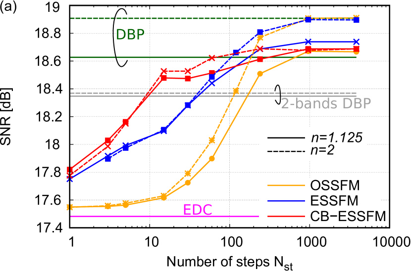
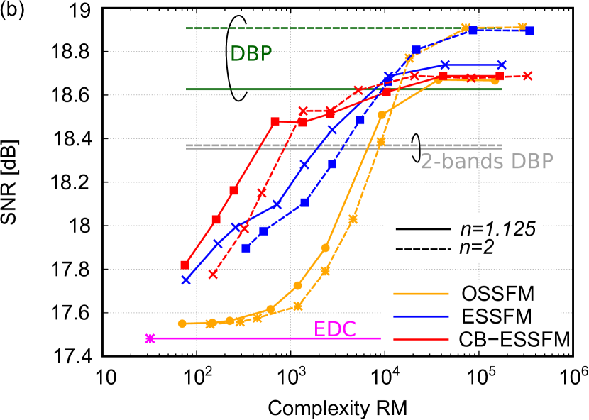
Figure 9: SNR for different DBP techniques and for $n=1.125$ (solid lines) and $n=2$ (dashed lines) (a) versus number of steps $N_{\text{st}}$, (b) versus complexity as number of real multiplications.

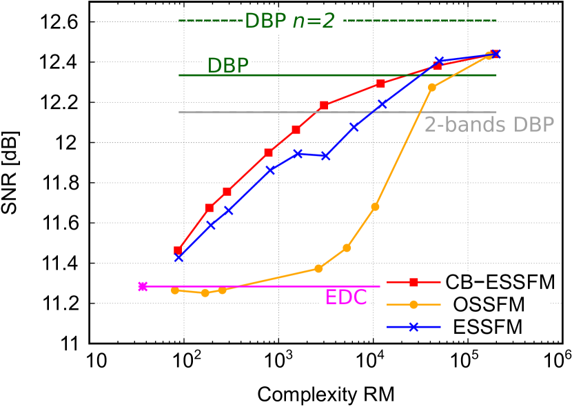
Figure 10: SNR with $60\times 80\,\mathrm{km}$ link for different DBP techniques and for $n=1.125$ (solid lines) and $n=2$ (dashed lines) versus complexity as number of real multiplications.

Next, Fig. 10 shows the performance versus complexity for the same configuration as Fig. 9(b) but considering $60$ spans of fiber, for an overall link length of $4800\,\mathrm{km}$. The behaviour is the same discussed for the $1200\,\mathrm{km}$link, but the complexity is in general higher, e.g., $10^{6}$ RM are not sufficient to achieve saturation for ESSFM and OSSFM. Furthermore, note that the largest gain of CB-ESSFM with respect to ESSFM is obtained again with one step per span, which, however, in this case corresponds to $N_{\text{st}}=60$, which corresponds approximately to $3\cdot 10^{3}$ RM.

Finally, Fig. 11 compares different DBP techniques as a function of the link length, when the number of spans, $80$km each, is $15$, $30$, $45$, and $60$. The performance of ideal DBP with $n=1.25$ and $n=2$ samples/symbol time and EDC are compared with those of the conventional symmetric ESSFM method (i.e., with $\rho=0.5$) and the CB-ESSFM method with $N_{\text{sb}}=2$ bands and optimized splitting ratio, both using $1$ step/span (i.e., $15$, $30$, $45$, and $60$ steps for the four considered lengths, respectively) and $n=1.125$. The figure show that the advantages of CB-ESSFM are maintained for different link lengths, when one step per span is used.

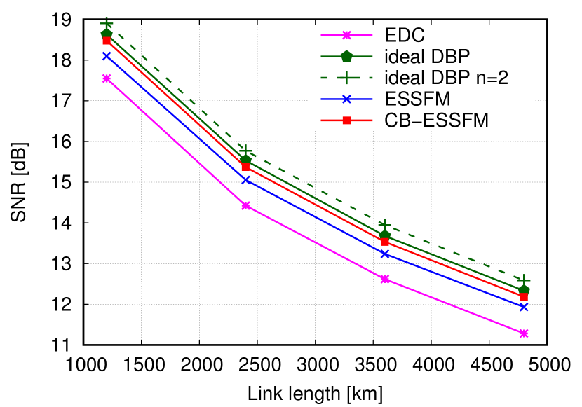
Figure 11: SNR versus link length for EDC, ideal DBP, ESSFM with $1$ step/span and $\rho=0.5$, and CB-ESSFM with $1$ step/span, $N_{\text{sb}}=2$ bands, and optimized $\rho$. $n=1.125$ except otherwise specified (dashed line ideal DBP $n=2$).

V Conclusion

A detailed analysis of novel methods and techniques for DBP for the compensation of inter-channel SPM nonlinear effects has been provided. In particular, a novel method—the coupled-band ESSFM (CB-ESSFM)—has been proposed. This method uses subband processing and nonlinear step optimization to obtain significant advantages in terms of performance versus complexity with respect to other DBP techniques.

The first part of this paper described the theoretical model for the propagation of a signal in an amplified fiber link, developed assuming an SSFM-like configuration consisting of several linear and nonlinear steps, and considering the FRLP model for the NLPR in each nonlinear step. The model is provided for the simplified single-band and single-polarization scenario, and then extended to multi-band and dual-polarization signals. The model serves as theoretical framework for several DBP models, including the ESSFM [9, 10], the CC-ESSFM [11, 12] and the CB-ESSFM, proposed here for the first time.

Next, in the second part it was described the implementation details of the CB-ESSFM using the overlap and save technique with variable nonlinear step position (splitting ratio), a numerical procedure to optimize offline the required coefficients, and a detailed analysis of the computational cost.

Finally, the performance of the CB-ESSFM has been shown by means of simulations. After showing the good agreement between CB-ESSFM coefficients obtained with analytical and numerical methods, the following results in terms of SNR were obtained.

• The CB-ESSFM improves on the ESSFM for low number of steps and symmetric configuration. The optimal number of subbands is $2$, with a gain of to $0.1$ dB for $N_{\text{st}}=15$ (both with $\rho=0.5$).

• The optimization of the position of the nonlinear steps provides some gain depending on the power profile in each step. The maximum gain for the CB-ESSFM is obtained when one step per span is used, with a gain of $0.29$ dB when $\rho=0.12$. In general, we observed that the nonlinear step should balance the accumulated nonlinearity in the two adjacent linear steps, and its optimization does not provide significant gains when less than one step per span is used.

• Overall, the CB-ESSFM provides a gain up to $0.38\,\mathrm{dB}$ w.r.t. the ESSFM with the same number of steps.

• The computational complexity of the CB-ESSFM is analyzed. With respect to EDC ($32\,\mathrm{RM/2D}$), the CB-ESSFM provides $0.34$dB gain with $75\,\mathrm{RM/2D}$, and 1 dB gain with $681\,\mathrm{RM/2D}$. Furthermore, the CB-ESSFM outperforms the ESSFM for the same number of operations, and it is advantageous to use a small number of samples per symbols.

• The same behavior is observed when longer links are considered, though the computational complexity increases, as expected. The largest improvement compared to our previously proposed ESSFM is obtained when one step per span is used, as in this case the optimization of the splitting ratio becomes critical.

Appendix A

According to the FRLP model, the propagation through the first half of the step in Fig. 1(a) can be approximated as [5, eq. (7)],

$$u^{\prime}(t) \approx\int_{-\infty}^{+\infty}U_{\mathrm{in}}(f)H(L/2,f)e^{-j\theta^{\prime}(f,t)}e^{j2\pi ft}df$$ (33)

where $U_{\mathrm{in}}(f)$ is the Fourier transform of $u_{\mathrm{in}}(t)$, $H(z,f)$ is given in (5), and $\theta^{\prime}(f,t)$ is a frequency- and time-dependent nonlinear phase rotation (NLPR) that accounts for SPM and its interaction with dispersion and attenuation [5, eq. (8)]. To further simplify the model, we neglect the frequency dependence of the NLPR and replace it with its value in the middle of the signal bandwidth, $\theta^{\prime}(t)\triangleq\theta^{\prime}(0,t)$. By letting $f=0$ in [5, eq. (8)], representing the input signal $U_{\mathrm{in}}(f)$ as a function of the linearly propagated signal $U(f)=U_{\mathrm{in}}(f)H(L/2,f)$, the NLPR can be expressed as

$$\theta^{\prime}(t)=P\iint_{\mathbb{R}^{2}}K^{\prime}(\mu,\nu)U(\mu)U^{*}(\nu)e^{j2\pi(\mu-\nu)t}\text{d}\mu\text{d}\nu$$ (34)

where

$$K^{\prime}(\mu,\nu)=\int_{-L/2}^{0}\gamma g(z)H(z,\mu)H^{*}(z,\nu)H^{*}(z,\mu-\nu)dz$$ (35)

is the kernel function, properly redifined with respect to [5, eq. (10)] to account for the additional approximation ($f=0$) and different normalizations used here. With this approximation, (33) can be rewritten as

$$u(t) =\int_{-\infty}^{+\infty}U_{\mathrm{in}}(f)H(L/2,f)e^{j2\pi ft}df$$ (36)

$$u^{\prime}(t) =e^{-j\theta^{\prime}(t)}u(t)$$ (37)

which can be interpreted as the cascade of the GVD and NLPR accumulated over the first half of the step, and represented by the first two blocks in Fig. 1(b). The propagation through the second half of the step in Fig. 1(a) is then approximated by a reverse-order FRLP model (with the NLPR preceding the GVD). This is obtained by using the same approximated FRLP model derived above to describe the backward propagation from $L/2$ to 0, obtaining

$$u^{\prime\prime}(t) =\int_{-\infty}^{+\infty}U_{\mathrm{out}}(f)H(-L/2,f)e^{j2\pi ft}df$$ (38)

$$u^{\prime}(t) =e^{-j\theta^{\prime\prime}(t)}u^{\prime\prime}(t)$$ (39)

where the NLPR is

$$\theta^{\prime\prime}(t) =P\iint_{\mathbb{R}^{2}}K^{\prime\prime}(\mu,\nu)U^{\prime\prime}(\mu)U^{\prime\prime*}(\nu)e^{j2\pi(\mu-\nu)t}\text{d}\mu\text{d}\nu$$

$$\approx P\iint_{\mathbb{R}^{2}}K^{\prime\prime}(\mu,\nu)U(\mu)U^{*}(\nu)e^{j2\pi(\mu-\nu)t}\text{d}\mu\text{d}\nu$$ (40)

with kernel function

$$K^{\prime\prime}(\mu,\nu)=\int_{L/2}^{0}\gamma g(z)H(z,\mu)H^{*}(z,\nu)H^{*}(z,\mu-\nu)dz$$ (41)

The approximation in (40) consists in replacing the potential $|u|^{2}$ that appears in the nonlinear term of the NLSE (1) and drives the generation of the NLPR with the intensity of the linearly propagated signal. This is the same approximation employed in [18, 5] to derive the original FRLP model in (33), so it is not expected to further reduce the accuracy of the final model. The forward propagation model for the second half of the step is obtained by inverting (38) and (39), obtaining

$$u^{\prime\prime}(t) =e^{j\theta^{\prime\prime}(t)}u^{\prime}(t)$$ (42)

$$u_{\mathrm{out}}(t) =\int_{-\infty}^{+\infty}U^{\prime\prime}(f)H(L/2,f)e^{j2\pi ft}df$$ (43)

corresponding, respectively, to the second NLPR and GVD blocks in Fig. 1(b). The model can be further simplified by combining the two adjacent NLPR blocks in Fig. 1(b) into a single block with overall NLPR $\theta(t)=\theta^{\prime}(t)-\theta^{\prime\prime}(t)$, as shown in Fig. 1(c), resulting in the overall propagation model (2)–(4), with kernel function $K(\mu,\nu)=K^{\prime}(\mu,\nu)-K^{\prime\prime}(\mu,\nu)$ given by (7).

Appendix B

We assume that $u(t)$ is band-limited, so that it can be represented as

$$u(t)=\sum_{k=-\infty}^{\infty}u[k]\text{sinc}\left(Rt-k\right)$$ (44)

where $u[k]=u(k/R)$ are its samples taken at sufficiently high rate $R=1/T$. By taking the Fourier transform of (44)

$$U(f)=\frac{1}{R}\sum_{k=-\infty}^{\infty}u[k]\text{rect}\left(f/R\right)\exp(-j2\pi kf/R)$$ (45)

and replacing it in (6), we can express the NLPR samples as

$$\theta[k] =\theta(k/R)$$

$$=(P/R^{2})\sum_{m=-\infty}^{\infty}\sum_{n=-\infty}^{\infty}u[m]u^{*}[n]$$

$$\times\int\limits_{-R/2}^{R/2}\int\limits_{R/2}^{R/2}K(\mu,\nu)e^{j2\pi[(k-m)\mu-(k-n)\nu)/R}d\mu d\nu$$

$$=\sum_{m=-\infty}^{\infty}\sum_{n=-\infty}^{\infty}d[k-m,k-n]u[m]u^{*}[n]$$

$$=\sum_{m=-\infty}^{\infty}\sum_{n=-\infty}^{\infty}d[m,n]u[k-m]u^{*}[k-n]$$ (46)

where

$$d[m,n]=\frac{P}{R^{2}}\int\limits_{-R/2}^{R/2}\int\limits_{-R/2}^{R/2}K(\mu,\nu)e^{j2\pi(m\mu-n\nu)/R}d\mu d\nu$$ (47)

are the coefficients of the discrete-time second-order Volterra kernel, corresponding to the samples of the inverse two-dimensional Fourier transform of the frequency-domain Volterra kernel (7) over a bandwidth equal to the sampling rate. After truncating the discrete-time Volterra kernel and neglecting its off-diagonal terms as discussed in Section II-A, we finally obtain the NLPR expression in (8) with the CB-ESSFM coefficients in (9).

In the multiband case, the derivation of the discrete-time model proceeds analogously. After dividing the signal $u(t)$ into $N_{\mathrm{sb}}$ subbands as in (10), the generic $i$th subband is represented as

$$u_{i}(t) =\sum_{k=-\infty}^{\infty}u_{i}[k]\text{sinc}\left(R^{\prime}t-k\right)\exp\left(j2\pi f_{i}t\right)$$ (48)

where $u_{i}[k]=u(k/R^{\prime})\exp(-j2\pi f_{i}k/R^{\prime})$ is the $k$th sample of the lowpass equivalent representation of the signal in the $i$th subband, taken at rate $R^{\prime}=R/N_{\mathrm{sb}}$. By replacing the Fourier transform of (48) in (12), truncating the discrete-time Volterra kernel and neglecting its off-diagonal terms as in the single-band case, we finaly obtain the NLPR expression in (13) with the CB-ESSFM coefficients in (14). The derivations of the dual-polarization discrete-time models (16) or (21)–(22) are very similar and are omitted.

Appendix C

By replacing (5) in (7), and defining

$$b\triangleq 2\pi^{2}\beta_{2}\nu(\mu-\nu)$$ (49)

the kernel function can be rewritten as

$$K(\mu,\nu)=\int_{-L/2}^{L/2}\gamma g(z)\exp(-j2bz)dz$$ (50)

For $N_{\mathrm{sp}}$ even, letting $\zeta=z-\left\lfloor z/L_{\mathrm{sp}}\right\rfloor\cdot L_{\mathrm{sp}}$, so that $g(z)=e^{-\alpha\zeta}$, we can rewrite (50) as

$$\sum_{n=-N_{\mathrm{sp}}/2}^{N_{\mathrm{sp}}/2-1}\exp(-j2bnL_{\mathrm{sp}})\int_{0}^{L_{\mathrm{sp}}}\gamma\exp[-(\alpha+j2b)\zeta]d\zeta$$

$$=\gamma\frac{1-e^{-(\alpha+j2b)L_{\mathrm{sp}}}}{\alpha+j2b}\sum_{n=-N_{\mathrm{sp}}/2}^{N_{\mathrm{sp}}/2-1}\exp(-j2bnL_{\mathrm{sp}})$$

$$=\gamma\frac{1-e^{-(\alpha+j2b)L_{\mathrm{sp}}}}{\alpha+j2b}\exp(jbN_{\mathrm{sp}}L_{\mathrm{sp}})\frac{1-\exp(-j2bN_{\mathrm{sp}}L_{\mathrm{sp}})}{1-\exp(-j2bL_{\mathrm{sp}})}$$ (51)

Eventually, after a few passages, we obtain the expression in (23) for the kernel function. The same result is obtained, with similar calculations, when $N_{\mathrm{sp}}$ is odd.

References

- [1] R.-J. Essiambre, G. Kramer, P. J. Winzer, G. J. Foschini, and B. Goebel, “Capacity limits of optical fiber networks,” J. Lightwave Technol., vol. 28, pp. 662–701, Feb. 2010.
- [2] P. J. Winzer, “Scaling optical fiber networks: Challenges and solutions,” Optics and Photonics News, vol. 26, no. 3, pp. 28–35, 2015.
- [3] G. P. Agrawal, Nonlinear Fiber Optics. Academic Press, 5th ed., 2013.
- [4] A. D. Ellis, J. Zhao, and D. Cotter, “Approaching the non-linear shannon limit,” Journal of lightwave technology, vol. 28, no. 4, pp. 423–433, 2009.
- [5] M. Secondini, E. Forestieri, and G. Prati, “Achievable information rate in nonlinear WDM fiber-optic systems with arbitrary modulation formats and dispersion maps,” J. Lightwave Technol., vol. 31, pp. 3839–3852, Dec. 2013.
- [6] T. Koike-Akino, C. Duan, K. Parsons, K. Kojima, T. Yoshida, T. Sugihara, and T. Mizuochi, “High-order statistical equalizer for nonlinearity compensation in dispersion-managed coherent optical communications,” Optics express, vol. 20, no. 14, pp. 15769–15780, 2012.
- [7] F. P. Guiomar and A. N. Pinto, “Simplified volterra series nonlinear equalizer for polarization-multiplexed coherent optical systems,” Journal of lightwave technology, vol. 31, no. 23, pp. 3879–3891, 2013.
- [8] D. Rafique, M. Mussolin, M. Forzati, J. Mårtensson, M. N. Chugtai, and A. D. Ellis, “Compensation of intra-channel nonlinear fibre impairments using simplified digital back-propagation algorithm,” Optics express, vol. 19, no. 10, pp. 9453–9460, 2011.
- [9] M. Secondini, D. Marsella, and E. Forestieri, “Enhanced split-step Fourier method for digital backpropagation,” in Proc. European Conf. Optical Commun. (ECOC), 2014.
- [10] M. Secondini, S. Rommel, G. Meloni, F. Fresi, E. Forestieri, and L. Poti, “Single-step digital backpropagation for nonlinearity mitigation,” Photon. Netw. Commun., vol. 31, pp. 493–502, June 2016.
- [11] S. Civelli, E. Forestieri, A. Lotsmanov, D. Razdoburdin, and M. Secondini, “Coupled-Channel Enhanced SSFM for Digital Backpropagation in WDM Systems,” in Proc. Optical Fiber Commun. Conf. (OFC), Optical Society of America, 2021.
- [12] S. Civelli, E. Forestieri, A. Lotsmanov, D. Razdoburdin, and M. Secondini, “Multichannel digital backpropagation with XPM-aware essfm,” in 17th International Symposium on Wireless Communication Systems (ISWCS), 2021.
- [13] V. Oliari, S. Goossens, C. Häger, G. Liga, R. M. Bütler, M. van den Hout, S. van der Heide, H. D. Pfister, C. Okonkwo, and A. Alvarado, “Revisiting efficient multi-step nonlinearity compensation with machine learning: An experimental demonstration,” Journal of Lightwave Technology, vol. 38, no. 12, pp. 3114–3124, 2020.
- [14] C. Häger and H. D. Pfister, “Wideband time-domain digital backpropagation via subband processing and deep learning,” in 2018 European Conference on Optical Communication (ECOC), pp. 1–3, IEEE, 2018.
- [15] S. Civelli, E. Forestieri, and M. Secondini, “Machine learning-aided nonlinearity-tailored carrier phase recovery for subcarrier multiplexing systems,” in Proc. Optical Fiber Commun. Conf. (OFC), Optica Publishing Group, 2024.
- [16] S. Luo, S. K. O. Soman, L. Lampe, and J. Mitra, “Deep learning-aided perturbation model-based fiber nonlinearity compensation,” Journal of Lightwave Technology, 2023.
- [17] E. Forestieri and M. Secondini, “Solving the nonlinear schrödinger equation,” Optical Communication Theory and Techniques, pp. 3–11, 2005.
- [18] M. Secondini and E. Forestieri, “Analytical fiber-optic channel model in the presence of cross-phase modulation,” IEEE Photonics Technology Letters, vol. 24, no. 22, pp. 2016–2019, 2012.
- [19] M. Secondini, “Chapter 20 - information capacity of optical channels,” in Optical Fiber Telecommunications VII (A. E. Willner, ed.), pp. 867–920, Academic Press, 2020.
- [20] G. P. Agrawal, Nonlinear Fiber Optics. San Diego, CA: Academic Press, 3rd ed., 2001.
- [21] C. R. Menyuk and B. S. Marks, “Interaction of polarization mode dispersion and nonlinearity in optical fiber transmission systems,” Journal of Lightwave Technology, vol. 24, no. 7, p. 2806, 2006.
- [22] M. Winter, C. A. Bunge, D. Setti, and K. Petermann, “A statistical treatment of cross-polarization modulation in DWDM systems,” J. Lightwave Technol., vol. 27, pp. 3739–3751, Sept. 2009.
- [23] M. Secondini, E. Agrell, E. Forestieri, D. Marsella, and M. R. Camara, “Nonlinearity mitigation in wdm systems: Models, strategies, and achievable rates,” J. Lightwave Technol., vol. 37, no. 10, pp. 2270–2283, 2019.
- [24] A. V. Oppenheim and R. W. Schafer, Discrete-time signal processing. Prentice Hall, 1999.
- [25] A. Wenzler and E. Luder, “New structures for complex multipliers and their noise analysis,” in 1995 IEEE International Symposium on Circuits and Systems (ISCAS), vol. 2, pp. 1432–1435, IEEE, 1995.
- [26] R. Yavne, “An economical method for calculating the discrete fourier transform,” in Proceedings of the December 9-11, 1968, fall joint computer conference, part I, pp. 115–125, 1968.
- [27] J. W. Cooley and J. W. Tukey, “An algorithm for the machine calculation of complex fourier series,” Mathematics of computation, vol. 19, no. 90, pp. 297–301, 1965.
- [28] S. Civelli, E. Forestieri, and M. Secondini, “Interplay of probabilistic shaping and carrier phase recovery for nonlinearity mitigation,” in Proc. European Conf. Optical Commun. (ECOC), IEEE, 2020.