Convexification for the 3D Problem of Travel Time Tomography

Abstract

The travel time tomography problem is a coefficient inverse problem for the eikonal equation. This problem has well known applications in seismic. The eikonal equation is considered here in the circular cylinder, where point sources run along its axis and measurements of travel times are conductes on the whole surface of this cylinder. A new version of the globally convergent convexification numerical method for this problem is developed. Results of numerical studies are presented.

Key Words: eikonal equation, geodesic lines, coefficient inverse problem, travel time tomography in 3d, globally convergent numerical method, Carleman estimate, numerical solution

2020 MSC codes: 35R30.

1 Introduction

The travel time tomography problem (TTTP) has a long history since it has broad applications in seismic studies of Earth, see, e.g. [21, 24]. First, we refer here to the pioneering works of Herglotz in 1905 [7] and Wiechert and Zoeppritz in 1907 [25], who have solved this problem in the 1d case. There are some important uniqueness and stability results for the TTTP. Since we are focused here on the numerical aspect, we cite only a few of those [17, 18, 19, 21]. We also refer to [22, 26] for numerical studies of the TTTP by the methods, which are significantly different from the convexification method of this paper.

Our goal here is to present the theory and computational experiments for a new version of the globally convergent convexification numerical method for the TTTP in the 3d case. The theory of the first version of the convexification for this problem was published in [12], [14, Chapter 11] and numerical studies were published in [15]. However, it was assumed in these references that the domain of interest $\Omega$ is a vertically elongated rectangular prism, and point sources run along an interval of a straight line, which is located in a horizontal plane “below” $\Omega.$ As a result, only horizontally oriented abnormalities were imaged in [15].

Since we do not want to be restricted to only horizontally oriented abnormalities, then we consider in this paper the case when $\Omega$ is a vertically oriented circular cylinder with point sources running along its axis and measurements of travel times being conducted on the lateral surface, top and bottom boundaries of this cylinder, see Figure 1. This source/detector configuration has applications in seismic imaging of wells. Naturally, our source/detector configuration requires some changes in the theory of [12, 15].

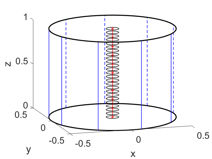
Figure 1: A schematic diagram of the source/detectors of this paper. The large circle is the outer boundary of the domain $\Omega$ defined in (3), the small circle is the inner boundary of domain $\Omega_{\varepsilon}$ defined in (4 ), and the red line with red star is position of the source $L_{\text{source}}$ defined in (5).

Below we first formulate and prove a new theorem about the monotonicity of the solution of the eikonal equation with respect to the radius of the cylindrical coordinate system. Next, using this theorem, we present a new version of the convexification method, which is adapted to the sources/detectors configuration of Figure 1. Next, we formulate some theorems of the convergence analysis. Since their close analogs were proven in [15], then we do not prove them here. Finally, we describe our numerical studies and present their results.

Definition. We call a numerical method for a Coefficient Inverse Problem (CIP) globally convergent, if there exists a theorem claiming that this method delivers points in a sufficiently small neighborhood of the true solution of that problem without any advanced knowledge of this neighborhood. The size of this neighborhood depends only on the noise level in the input data for this CIP. In other words, a good first guess about the true solution is not required.

The first theoretical results about the convexification method for CIPs were obtained in [9, 10]. More recent works on this method for various CIPs contain both theory and numerical results, see, e.g. [1, 2, 13, 14, 15, 16] and references cited therein. The development of the convexification is caused by the desire to avoid the phenomenon of local minima and ravines of conventional least squares cost functionals for CIPs, see, e.g. [3, 4, 5]. In the convexification, a globally strongly cost functional is constructed. The key element of this functional is the presence of the Carleman Weight Function (CWF) in it. This is the function, which is used as the weight in the Carleman estimate for an associated operator. Usually this is a partial differential operator. In the case of the TTTP, however, this is a Volterra-like integral operator. Finally, it is proven that the gradient descent method of the minimization of this functional converges globally to the true solution of the corresponding CIP as long as the level of noise in the data tends to zero.

All functions considered below are real valued ones. In section 2 we pose our inverse problem. In section 3 we prove the above mentioned important theorem about the monotonicity of the travel time function with respect to the radius of the cylindrical coordinate system. In section 4 we derive an integral differential equation, which does not contain the unknown coefficient. In section 5 we present an important element of our method: the orthonormal basis of [11], [14, section 6.2.3]. In section 6 we derive a boundary value problem and also prove a Carleman estimate for the Volterra integral operator. In section 7 we introduce partial finite differences for our problem. In section 8 we present the convexification functional and formulate theorems of its global convergence analysis. Section 9 is devoted to numerical studies.

2 Statement of the Problem

Below $\mathbf{x}=\left(x,y,z\right)$ denotes points in $\mathbb{R}^{3}.$ Let $c\left(\mathbf{x}\right)$ be the speed of waves propagation, $c\left(\mathbf{x}\right)=1/n\left(\mathbf{x}\right)$, where $n\left(\mathbf{x}\right)$ is the refractive index. The function $n\left(\mathbf{x}\right)$ generates the Riemannian metric [21, Chapter 3]

(1) $$d\tau=n\left(\mathbf{x}\right)\sqrt{\left(dx\right)^{2}+\left(dy\right)^{2}+\left(dz\right)^{2}}.$$

Let $\mathbf{x}_{0}$ be a source of waves and $\mathbf{x}$ be an observation point. The time, which the wave needs to propagate from a source $\mathbf{x}_{0}$ to a point $\mathbf{x,}$ is called the “first arrival time” or “travel time”. In the case of a heterogeneous medium with $n\left(\mathbf{x}\right)\neq const.,$ the first arriving signal, which arrives at the arrival time to the point $\mathbf{x}$, travels along the so-called “geodesic line” $\Gamma\left(\mathbf{x},\mathbf{x}_{0}\right)$ generated by metric (1). The first arrival time $\tau\left(\mathbf{x},\mathbf{x}_{0}\right)$ is

$$\tau\left(\mathbf{x},\mathbf{x}_{0}\right)=\int\limits_{\Gamma\left(\mathbf{x},\mathbf{x}_{0}\right)}n\left(\mathbf{y}\left(s\right)\right)d\sigma,$$

where $d\sigma$ is the element of the euclidean length. The function $\tau\left(\mathbf{x},\mathbf{x}_{0}\right)$ satisfies the following eikonal equation [21, Chapter 3]:

(2) $$\begin{split}&\hskip 28.45274pt\left(\nabla_{\mathbf{x}}\tau\right)^{2}=n^{2}\left(\mathbf{x}\right),\\ &\tau\left(\mathbf{x},\mathbf{x}_{0}\right)=O\left(\left|\mathbf{x}-\mathbf{x}_{0}\right|\right)\text{ as }\mathbf{x}\rightarrow\mathbf{x}_{0}.\end{split}$$

Consider two numbers $R,B>0$ and let $\varepsilon\in\left(0,R\right)$ be a small number. We define the domains $\Omega,\Omega_{\varepsilon}\subset\mathbb{R}^{3}$ as:

(3) $$\Omega=\left\{\mathbf{x}=\left(x,y,z\right):\sqrt{x^{2}+y^{2}}<R,z\in\left(0,B\right)\right\},$$

(4) $$\Omega_{\varepsilon}=\left\{\mathbf{x}=\left(x,y,z\right):\sqrt{x^{2}+y^{2}}<\varepsilon,z\in\left(0,B\right)\right\},$$

(5) $$\hskip 5.69046ptL_{\text{source}}=\left\{\mathbf{x}_{0}=\left(x_{0},y_{0},z_{0}\right):x_{0}=y_{0}=0,z_{0}\in\left(0,B\right)\right\}.$$

Hence, $\Omega$ and $\Omega_{\varepsilon}$ are vertically oriented cylinders with the radii $R$ and $\varepsilon$ respectively, $\Omega_{\varepsilon}\subset\Omega,$ and $L_{\text{source}}$ is the vertical axis of both cylinders, along which sources $\mathbf{x}_{0}$ run.

Consider the cylindrical coordinates $\mathbf{x}=\left(x,y,z\right)=\left(r\cos\varphi,r\sin\varphi,z\right).$ Therefore by (3) and (4) in cylindrical coordinates

(6) $$\Omega=\left\{\left(r,\varphi,z\right):r\in\left(0,R\right),\varphi\in[0,2\pi),z\in\left(0,B\right)\right\},$$

(7) $$\Omega_{\varepsilon}=\left\{\left(r,\varphi,z\right):r\in\left(0,\varepsilon\right),\varphi\in[0,2\pi),z\in\left(0,B\right)\right\},$$

(8) $$\hskip 14.22636ptD=\Omega\diagdown\Omega_{\varepsilon}=\left\{\left(r,\varphi,z\right):r\in\left(\varepsilon,R\right),\varphi\in[0,2\pi),z\in\left(0,B\right)\right\}.$$

We consider below the eikonal equation (2) only in the domain $\Omega.$ We assume that the refractive index $n(\mathbf{x})$ satisfies the following conditions:

(9) $$n(\mathbf{x}) =1\text{ in }\Omega_{\varepsilon},$$

(10) $$n(\mathbf{x}) \in C^{1}\left(\overline{\Omega}\right),$$

(11) $$n_{r}\left(r,\varphi,z\right) \geq 0\text{ in }\Omega.$$

In cylindrical coordinates eikonal equation (2) has the form

(12) $$(\tau_{r})^{2}+\frac{1}{r^{2}}(\tau_{\varphi})^{2}+(\tau_{z})^{2}=n^{2}(r,\varphi,z).$$

By (5) denote

(13) $$\tau\left(\mathbf{x,x}_{0}\right)=\tau\left(\mathbf{x,}z_{0}\right),\text{ }\mathbf{x}_{0}\in L_{\text{source}},\text{ }z_{0}\in\left(0,B\right).$$

Travel Time Tomography Problem (TTTP). Let conditions (3)-(13) hold. Find the refractive index $n\left(\mathbf{x}\right)$ for $\mathbf{x}\in D,$ assuming that the following functions $p\left(\varphi,z,z_{0}\right)$, $p_{0}\left(r,\varphi,z_{0}\right),p_{B}\left(r,\varphi,z_{0}\right)$ are known:

(14) $$p\left(\varphi,z,z_{0}\right) =\tau\left(R,\varphi,z,z_{0}\right),\text{ }\forall\varphi\in\left(0,2\pi\right),\forall z,z_{0}\in\left(0,B\right),$$

(15) $$p_{0}\left(r,\varphi,z_{0}\right) =\tau\left(r,\varphi,0,z_{0}\right),\forall r\in\left(\varepsilon,R\right),\text{ }\forall\varphi\in\left(0,2\pi\right),\forall z_{0}\in\left(0,B\right),$$

(16) $$p_{B}\left(r,\varphi,z_{0}\right) =\tau\left(r,\varphi,B,z_{0}\right),\forall r\in\left(\varepsilon,R\right),\forall\varphi\in\left(0,2\pi\right),\forall z_{0}\in\left(0,B\right).$$

Everywhere below we assume that the following condition is valid:

Assumption of the Regularity of Geodesic Lines. For any pair of points $\left(\mathbf{x},\mathbf{x}_{0}\right)\in\overline{\Omega}\times L_{\text{source}}$ there exists unique geodesic line $\Gamma\left(\mathbf{x},\mathbf{x}_{0}\right)$ connecting these two points.

3 The Monotonicity Property of the Function $\tau\left(r,\varphi,z,z_{0}\right)$

Theorem 3.1. Assume that conditions (3)-(11) are in place. Then the following inequality is valid:

(17) $$\tau_{r}\left(r,\varphi,z,z_{0}\right)\geq\frac{\varepsilon}{\sqrt{\varepsilon^{2}+B^{2}}}=c,\text{ }\forall\left(r,\varphi,z\right)\in\overline{D}.$$

Proof. Denote $\tau_{r}=q_{1}$, $\tau_{\varphi}=q_{2}$, $\tau_{z}=q_{3}$. Then the eikonal equation (12) becomes: 

(18) $$q_{1}^{2}+\frac{1}{r^{2}}q_{2}^{2}+q_{3}^{2}=n^{2}(r,\varphi,z).$$

Differentiating (18) with respect to $r,\varphi,z$ and using the equalities

$$\left.\begin{array}[]{c}(q_{2})_{r}=(q_{1})_{\varphi},\quad(q_{3})_{r}=(q_{1})_{z},(q_{1})_{\varphi}=(q_{2})_{r},(q_{3})_{\varphi}=(q_{2})_{z},(q_{2})_{z}=(q_{3})_{\varphi},\end{array}\right.$$

we obtain that along the geodesic line $\Gamma\left(\mathbf{x},\mathbf{x}_{0}\right)$ with $\mathbf{x}_{0}=(0,0,z_{0})$

(19) $$\frac{dr}{ds}=\frac{q_{1}}{n^{2}},\text{ }\frac{d\varphi}{ds}=\frac{q_{2}}{r^{2}n^{2}},\text{ }\frac{dz}{ds}=\frac{q_{3}}{n^{2}},$$

(20) $$\frac{dq_{1}}{ds}=\frac{n_{r}}{n}+\frac{q_{2}^{2}}{r^{3}n},\text{ }\frac{dq_{2}}{ds}=\frac{n_{\varphi}}{n},\text{ }\frac{dq_{3}}{ds}=\frac{n_{z}}{n},\text{ }\frac{d\tau}{ds}=1,$$

where $ds$ is the element of the Riemannian length of $\Gamma\left(\mathbf{x},\mathbf{x}_{0}\right)$.

Equations (19), (20) form a coupled system of ordinary differential equations. We need to figure out initial conditions for this system. Consider the geodesic line $\Gamma\left(r,\varphi,z,\mathbf{x}_{0}\right)$ that connects the point $\mathbf{x}_{0}=(0,0,z_{0})$ with the point $(r,\varphi,z).$ The tangent vector to this line at the point $\mathbf{x}_{0}$ is the vector

$\nu_{0}=(\sin\theta_{0}\cos\varphi_{0}$, $\sin\theta_{0}\sin\varphi_{0}$, $\cos\theta_{0})$. Hence, the initial conditions for this geodesic line are:

(21) $$r|_{s=0}=0,\quad \varphi|_{s=0}=\varphi_{0},\quad z|_{s=0}=z_{0},$$

(22) $$(q_{1})_{s=0}=\sin\theta_{0},\quad (q_{2})_{s=0}=0,\quad(q_{3})_{s=0}=\cos\theta_{0}.$$

Thus, solving Cauchy problem (19)-(22), we obtain equations of $\Gamma\left(\left(r,\varphi,z\right),\left(0,0,z_{0}\right)\right)$ in the parametric form

$$r=r(s,z_{0},\theta_{0},\varphi_{0}),\quad\varphi=\varphi(s,z_{0},\theta_{0},\varphi_{0}),\quad z=z(s,z_{0},\theta_{0},\varphi_{0}).$$

Due to the regularity of geodesic lines, there exists a one-to-one correspondence between points $\left(0,0,z_{0}\right)$ and $(r,\varphi,z).$ In particular, this means that for any fixed $z_{0}$ there exists a one-to-one correspondence between $(r,\varphi,z)$ and parameters $(s,\theta_{0},\varphi_{0})$.  We denote this correspondence as:

$$s=s(r,\varphi,z,z_{0})\equiv\tau(r,\varphi,z,z_{0}),\quad\theta_{0}=\theta_{0}(r,\varphi,z,z_{0}),\quad\varphi_{0}=\varphi_{0}(r,\varphi,z,z_{0}).$$

Moreover, we have along the geodesic line $\Gamma\left(\left(r,\varphi,z\right),\left(0,0,z_{0}\right)\right):$

(23) $$\frac{dq_{1}}{ds}=\frac{d\tau_{r}}{ds}=\frac{n_{r}}{n}+\frac{q_{2}^{2}}{r^{3}n^{2}}\geq 0.$$

For any point $\left(r,\varphi,z\right)\in\overline{\Omega}\diagdown\Omega_{\varepsilon}$ the geodesic line $\Gamma\left(r,\varphi,z,\mathbf{x}_{0}\right)$ is:

$$\Gamma\left(r,\varphi,z,\mathbf{x}_{0}\right)=\Gamma_{\varepsilon}\left(r,\varphi,z,\mathbf{x}_{0}\right)\cup\Gamma_{1}\left(r,\varphi,z,\mathbf{x}_{0}\right),$$

where

(24) $$\Gamma_{\varepsilon}\left(r,\varphi,z,\mathbf{x}_{0}\right)=\Gamma\left(r,\varphi,z,\mathbf{x}_{0}\right)\cap\Omega_{\varepsilon}\text{ and }\Gamma_{1}\left(r,\varphi,z,\mathbf{x}_{0}\right)\subset\overline{D}.$$

By (9) $\Gamma_{\varepsilon}\left(r,\varphi,z,\mathbf{x}_{0}\right)$ is a part of a straight line. Let $\left(\varepsilon,\varphi^{\ast},z^{\ast}\right)$ be the intersection of $\Gamma_{\varepsilon}(\mathbf{x,x}_{0})$ with the lateral boundary $\left\{r=\varepsilon,z\in\left(0,B\right)\right\}$ of the cylinder $\Omega_{\varepsilon}.$ Then $\tau\left(r,\varphi^{\ast},z^{\ast},z_{0}\right)=\sqrt{r^{2}+\left(z^{\ast}-z_{0}\right)^{2}}$ for $r\in\left(0,\varepsilon\right).$ Hence,

(25) $$\tau_{r}\left(\varepsilon,\varphi^{\ast},z^{\ast},z_{0}\right)=\frac{\varepsilon}{\sqrt{\varepsilon^{2}+\left(z^{\ast}-z_{0}\right)^{2}}}\geq\frac{\varepsilon}{\sqrt{\varepsilon^{2}+B^{2}}}.$$

Hence, by (11), (20) and (25) for $\left(r,\varphi,z\right)\in\overline{\Omega}\diagdown\Omega_{\varepsilon}$

$$\tau_{r}\left(r,\varphi,z,z_{0}\right)=\int\limits_{\sqrt{\varepsilon^{2}+\left(z^{\ast}-z_{0}\right)^{2}}}^{s} \left(\frac{n_{r}}{n}+\frac{q_{2}^{2}}{r^{3}n^{2}}\right)ds+\frac{\varepsilon}{\sqrt{\varepsilon^{2}+\left(z^{\ast}-z_{0}\right)^{2}}}\geq$$

$$\geq\frac{\varepsilon}{\sqrt{\varepsilon^{2}+B^{2}}}=c.\text{ \ }\square$$

4 Integral Differential Equation

Denote

(26) $$\left.\begin{array}[]{c}u\left(r,\varphi,z,z_{0}\right)=\tau_{r}^{2}\left(r,\varphi,z,z_{0}\right),\ \left(r,\varphi,z\right)\in D,z_{0}\in\left(0,B\right).\end{array}\right.$$

Since by Theorem 3.1 $\tau_{r}\left(r,\varphi,z,z_{0}\right)\geq c>0,$ then  by (26)

(27) $$\tau_{r}\left(r,\varphi,z,z_{0}\right)=\sqrt{u\left(r,\varphi,z,z_{0}\right)}.$$

Hence, (14) and (27) imply

(28) $$\left.\begin{array}[]{c}\tau\left(r,\varphi,z,z_{0}\right)=-\int\limits_{r}^{R}\sqrt{u\left(t,\varphi,z,z_{0}\right)}dt+p\left(\varphi,z,z_{0}\right),\\ \tau\left(r,\varphi,0,z_{0}\right)=p_{0}\left(r,\varphi,z_{0}\right),\ \tau\left(r,\varphi,B,z_{0}\right)=p_{B}\left(r,\varphi,z_{0}\right),\\ \left(r,\varphi,z,z_{0}\right)\in Q=\left(\varepsilon,R\right)\times\left(0,2\pi\right)\times\left(0,B\right)\times\left(0,B\right).\end{array}\right.$$

By the first line of (28)

(29) $$\tau_{\varphi}\left(r,\varphi,z,z_{0}\right) =-\frac{1}{2}\int\limits_{r}^{R}\frac{u_{\varphi}\left(t,\varphi,z,z_{0}\right)}{\sqrt{u\left(t,\varphi,z,z_{0}\right)}}dt+p_{\varphi}\left(\varphi,z,z_{0}\right),$$

(30) $$\tau_{z}\left(r,\varphi,z,z_{0}\right) =-\frac{1}{2}\int\limits_{r}^{R}\frac{u_{z}\left(t,\varphi,z,z_{0}\right)}{\sqrt{u\left(t,\varphi,z,z_{0}\right)}}dt+p_{z}\left(\varphi,z,z_{0}\right).$$

Substituting (28)-(30) in the eikonal equation (12), we obtain the following equation in the domain $Q$ defined in the last line of (28):

$$u\left(r,\varphi,z,z_{0}\right)+\frac{1}{r^{2}}\left[-\frac{1}{2}\int\limits_{r}^{R}\frac{u_{\varphi}\left(t,\varphi,z,z_{0}\right)}{\sqrt{u\left(t,\varphi,z,z_{0}\right)}}dt+p_{\varphi}\left(\varphi,z,z_{0}\right)\right]^{2}+$$

(31) $$+\left[-\frac{1}{2}\int\limits_{r}^{R}\frac{u_{z}\left(t,\varphi,z,z_{0}\right)}{\sqrt{u\left(t,\varphi,z,z_{0}\right)}}dt+p_{z}\left(\varphi,z,z_{0}\right)\right]^{2}=n^{2}(r,\varphi,z).$$

Differentiating (31) with respect to $z_{0}$ and using $\partial_{z_{0}}\left[n^{2}(r,\varphi,z)\right]\equiv 0,$ we obtain

$$u_{z_{0}}\left(r,\varphi,z,z_{0}\right)+\frac{1}{r^{2}}\frac{\partial}{\partial z_{0}}\left[-\frac{1}{2}\int\limits_{r}^{R}\frac{u_{\varphi}\left(t,\varphi,z,z_{0}\right)}{\sqrt{u\left(t,\varphi,z,z_{0}\right)}}dt+p_{\varphi}\left(\varphi,z,z_{0}\right)\right]^{2}+$$

(32) $$+\frac{\partial}{\partial z_{0}}\left[-\frac{1}{2}\int\limits_{r}^{R}\frac{u_{z}\left(t,\varphi,z,z_{0}\right)}{\sqrt{u\left(t,\varphi,z,z_{0}\right)}}dt+p_{z}\left(\varphi,z,z_{0}\right)\right]^{2}=0.$$

In addition, (15), (16) and (26) imply:

(33) $$u\left(r,\varphi,0,z_{0}\right)=\left(\partial_{r}p_{0}\left(r,\varphi,z_{0}\right)\right)^{2},\text{ }u\left(r,\varphi,B,z_{0}\right)=\left(\partial_{r}p_{B}\left(r,\varphi,z_{0}\right)\right)^{2}.$$

In (31)-(33)

(34) $$\left(r,\varphi,z,z_{0}\right)\in\overline{Q}.$$

Thus, we came up with the following boundary value problem (BVP).

Boundary Value Problem 1 (BVP1). Find the function $u\left(r,\varphi,z,z_{0}\right)\in C^{1}\left(\overline{Q}\right)$  satisfying conditions (32), (33) in the domain (34).

Suppose that we have solved this problem. Then we substitute its solution in the left hand side of equation (31) and find the target function $n(r,\varphi,z).$ Clearly BVP1 is a very complicated one. Therefore, we construct below an approximate mathematical model for its solution, and then confirm the validity of this model computationally.

5 A Special Orthonormal Basis in $L_{2}\left(0,B\right)$

The basis described in this section was first introduced in [11]. Then it was used for the convexification method in some other works, see, e.g. [12, 14, 15]. Consider the set of functions $\{z_{0}^{n}e^{z_{0}}\}_{n=0}^{\infty}\subset L_{2}(0,B).$ Obviously, this set is complete in $L_{2}(0,B),$ and these functions are linearly independent. Apply the Gram-Schmidt orthonormalization procedure to this set. Then we obtain the orthonormal basis $\{\Psi_{n}\left(z_{0}\right)\}_{n=0}^{\infty}$ in $L_{2}(0,B)$. The function $\Psi_{n}(z_{0})$ has the form $\Psi_{n}(z_{0})=P_{n}(z_{0})e^{z_{0}}$, $\forall n\geq 0,$ where $P_{n}(z_{0})$ is a polynomial of the degree $n$. Denote

$$a_{mn}=\int\limits_{0}^{B}\Phi_{m}\left(z_{0}\right),\Phi_{n}^{\prime}\left(z_{0}\right)dz_{0}.$$

It was proven in [11], [14, Theorem 6.2.1] that

(35) $$a_{mn}=\left\{\begin{array}[]{c}1\text{ if }m=n,\\ 0\text{ if }m>n.\end{array}\right.$$

Let $N\geq 1$ be an integer. Consider the $N\times N$ matrix $A_{N}=\left(a_{mn}\right)_{m,n=0}^{N}.$ By (35) $\det A_{N}=1.$ Hence, the matrix $A_{N}$ is invertible. We observe that neither classical orthonormal polynomials nor the basis of trigonometric functions do not provide a corresponding invertible matrix $A_{N}$. This is because the first function in these two cases is an identical constant, implying that the first column of that analog of $A_{N}$ is formed only by zeros.

6 Boundary Value Problem 2

The first step of our approximate mathematical model mentioned in section 4 is the assumption that the function $u$ can be represented as truncated Fourier-like series,

(36) $$u\left(r,\varphi,z,z_{0}\right)=\sum\limits_{s=0}^{N-1}u_{s}\left(r,\varphi,z\right)\Phi_{s}\left(z_{0}\right),\text{ }\left(r,\varphi,z,z_{0}\right)\in Q.$$

We do not prove convergence of our method as $N\rightarrow\infty.$ We point out that the absence of such proofs is a rather common place in the theory of Inverse Problems, basically due to their ill-posedness, see, e.g. [6, 8].

Consider the $N-$D vector function $V\left(r,\varphi,z\right)$ of coefficients of the series (36)

(37) $$\left.\begin{array}[]{c}V\left(r,\varphi,z\right)=\left(u_{0},...,u_{N-1}\right)^{T}\left(r,\varphi,z\right),\text{ }\\ \left(r,\varphi,z\right)\in\left(\varepsilon,R\right)\times\left(0,2\pi\right)\times\left(0,B\right).\end{array}\right.$$

We want to find the vector function $V\left(r,\varphi,z\right)$ in (37). Naturally, we assume that for functions in (14)-(16)

(38) $$\left.\begin{array}[]{c}p\left(\varphi,z,z_{0}\right)=\sum\limits_{s=0}^{N-1}p_{s}\left(\varphi,z\right)\Phi_{s}\left(z_{0}\right),\\ \left(\varphi,z,z_{0}\right)\in\left(0,2\pi\right)\times\left(0,B\right)\times\left(0,B\right).\end{array}\right.$$

(39) $$\left.\begin{array}[]{c}\left(\partial_{r}p_{0}\right)^{2}\left(r,\varphi,z_{0}\right)=\sum\limits_{s=0}^{N-1}\widetilde{p}_{0,s}\left(r,\varphi\right)\Phi_{s}\left(z_{0}\right),\\ \left(\partial_{r}p_{B}\right)^{2}\left(r,\varphi,z_{0}\right)=\sum\limits_{s=0}^{N-1}\widetilde{p}_{B,s}\left(r,\varphi\right)\Phi_{s}\left(z_{0}\right),\\ \left(r,\varphi,z_{0}\right)\in\left(\varepsilon,R\right)\times\left(0,2\pi\right)\times\left(0,B\right).\end{array}\right.$$

Denote

(40) $$\left.\begin{array}[]{c}G\left(\varphi,z\right)=\left(p_{0},...,p_{N-1}\right)^{T}\left(\varphi,z\right),\quad\left(\varphi,z\right)\in\left(0,2\pi\right)\times\left(0,B\right),\\ \text{ }G_{0}\left(r,\varphi\right)=\left(\widetilde{p}_{0,0},...\widetilde{p}_{0,N-1}\right)^{T}\left(r,\varphi\right),\text{ }\left(r,\varphi\right)\in\left(\varepsilon,R\right)\times\left(0,2\pi\right)\\ G_{B}\left(r,\varphi\right)=\left(\widetilde{p}_{B,0},...\widetilde{p}_{B,N-1}\right)^{T}\left(r,\varphi\right),\text{ }\left(r,\varphi\right)\in\left(\varepsilon,R\right)\times\left(0,2\pi\right).\end{array}\right.$$

Substituting (36)-(40) in (32), multiplying the obtained equality sequentially by the functions $\Psi_{n}\left(z_{0}\right),n=0,...,N-1$ and integrating with respect to $z_{0}\in\left(0,B\right),$ we obtain

(41) $$\left.\begin{array}[]{c}A_{N}V+S\left(V_{\varphi},V_{z},G,r,\varphi,z\right)=0,\\ V\left(r,\varphi,0\right)=\text{ }G_{0}\left(r,\varphi\right),\\ V\left(r,\varphi,B\right)=\text{ }G_{B}\left(r,\varphi\right),\\ V\left(r,0,z\right)=V\left(r,2\pi,z\right),\\ \left(r,\varphi,z\right)\in\left(\varepsilon,R\right)\times\left(0,2\pi\right)\times\left(0,B\right),\end{array}\right.$$

where $S\in\mathbb{R}^{N}$ is a $C^{1}-$vector function of its $3N+3$ arguments. The fourth line in (41) means the $2\pi-$periodicity condition with respect to the angle $\varphi.$ Thus, (41) is the boundary value problem for the nonlinear system of integral differential equations with respect to the vector function $V\left(r,\varphi,z\right).$ Here, the $s-$th component of the $N-$D vector function $S=\left(S_{0},...,S_{N-1}\right)^{T}$ has the form

$$S_{s}\left(V_{\varphi},V_{z},r\right)=S_{s}^{\varphi}\left(V_{\varphi},V_{z},r\right)+S_{s}^{z}\left(V_{\varphi},V_{z},r\right).$$

Here $S_{n}^{\varphi}\left(V_{\varphi},V_{z},G_{\varphi},G_{z},r\right)$ has the following form after the integration by parts with respect to $z_{0}$:

$$S_{s}^{\varphi}\left(V_{\varphi},V_{z},r\right)= \Psi_{s}\left(B\right)\frac{1}{r^{2}}\left[-\frac{1}{2}\int\limits_{r}^{R}\frac{u_{\varphi}\left(t,\varphi,z,B\right)}{\sqrt{u\left(t,\varphi,z,B\right)}}dt+p_{\varphi}\left(\varphi,z,B\right)\right]^{2}-$$

(42) $$-\Psi_{s}\left(0\right)\frac{1}{r^{2}} \left[-\frac{1}{2}\int\limits_{r}^{R}\frac{u_{\varphi}\left(t,\varphi,z,0\right)}{\sqrt{u\left(t,\varphi,z,0\right)}}dt+p_{\varphi}\left(\varphi,z,0\right)\right]^{2}-$$

$$-\frac{1}{r^{2}}\int\limits_{0}^{B}\Psi_{s}^{\prime} \left(z_{0}\right)\left[-\frac{1}{2}\int\limits_{r}^{R}\frac{u_{\varphi}\left(t,\varphi,z,z_{0}\right)}{\sqrt{u\left(t,\varphi,z,z_{0}\right)}}dt+p_{\varphi}\left(\varphi,z,z_{0}\right)\right]^{2}dz_{0}.$$

And $S_{s}^{z}\left(V_{\varphi},V_{z},G_{\varphi},G_{z},r\right)$ has the form after the integration by parts with respect to $z_{0}$:

(43) $$S_{s}^{z}\left(V_{\varphi},V_{z},r\right)= \Psi_{s}\left(B\right)\left[-\frac{1}{2}\int\limits_{r}^{R}\frac{u_{z}\left(t,\varphi,z,B\right)}{\sqrt{u\left(t,\varphi,z,B\right)}}dt+p_{z}\left(\varphi,z,B\right)\right]^{2}-$$

$$-\Psi_{s}\left(0\right) \left[-\frac{1}{2}\int\limits_{r}^{R}\frac{u_{z}\left(t,\varphi,z,0\right)}{\sqrt{u\left(t,\varphi,z,0\right)}}dt+p_{z}\left(\varphi,z,0\right)\right]^{2}-$$

$$-\int\limits_{0}^{B}\Psi_{s}^{\prime} \left(z_{0}\right)\left[-\frac{1}{2}\int\limits_{r}^{R}\frac{u_{z}\left(t,\varphi,z,z_{0}\right)}{\sqrt{u\left(t,\varphi,z,z_{0}\right)}}dt+p_{z}\left(\varphi,z,z_{0}\right)\right]^{2}dz_{0}.$$

In (42), (43) the function $u$ has the form (36), and the vector function $V$ has the form (37). Thus, we have obtained Boundary Value Problem 2 (BVP2).

Boundary Value Problem 2 (BVP2). Let $D$ be the domain defined in (8). Find the $N-$D vector function $V\in C^{1}\left(\overline{D}\right)$ satisfying conditions (41), where the function $u$ is connected with $V$ via (36), (37).

We now formulate a Carleman estimate for the Volterra integral operator occurring in (41)-(43). First, we introduce the Carleman Weight Function $\varphi_{\lambda}\left(r\right)$ for this Volterra operator, where $\lambda>0$ is a parameter. This function is:

(44) $$\varphi_{\lambda}\left(r\right)=e^{2\lambda r}.$$

Theorem 6.1 (Carleman estimate for the Volterra integral operator). The following Carleman estimate is valid:

(45) $$\int\limits_{\varepsilon}^{R}\left(\int\limits_{r}^{R}f\left(s\right)ds\right)^{2}e^{2\lambda r}dr\leq\frac{1}{\lambda^{2}}\int\limits_{\varepsilon}^{R}f^{2}\left(r\right)e^{2\lambda r}dr,\text{ }\forall\lambda>0,\text{ }\forall f\in L_{2}\left(\varepsilon,R\right).$$

Proof. Integrating by parts and using Cauchy-Schwarz inequality, we obtain

$$\int\limits_{\varepsilon}^{R}\left(\int\limits_{r}^{R}f\left(s\right)ds\right)^{2}e^{2\lambda r}dr=-\frac{1}{2\lambda}\left(\int\limits_{\varepsilon}^{R}f\left(s\right)ds\right)^{2}e^{2\lambda\varepsilon}dr+$$

$$\hskip 28.45274pt+\frac{1}{\lambda}\int\limits_{\varepsilon}^{R}\left[e^{\lambda r}\int\limits_{r}^{R}f\left(s\right)ds\right]\left[f\left(r\right)e^{\lambda r}\right]dr\leq$$

$$\leq\frac{1}{\lambda}\left[\int\limits_{\varepsilon}^{R}\left(\int\limits_{r}^{R}f\left(s\right)ds\right)^{2}e^{2\lambda r}dr\right]^{1/2}\left[\int\limits_{\varepsilon}^{R}f^{2}\left(r\right)e^{2\lambda r}dr\right]^{1/2}.$$

Thus, we have proven that

(46) $$\left.\begin{array}[]{c}\int\limits_{\varepsilon}^{R}\left(\int\limits_{r}^{R}f\left(s\right)ds\right)^{2}\varphi_{\lambda}\left(r\right)dr\leq\\ \leq\left(1/\lambda\right)\left[\int\limits_{\varepsilon}^{R}\left(\int\limits_{r}^{R}f\left(s\right)ds\right)^{2}\varphi_{\lambda}\left(r\right)dr\right]^{1/2}\left[\int\limits_{\varepsilon}^{R}f^{2}\left(r\right)\varphi_{\lambda}\left(r\right)dr\right]^{1/2}.\end{array}\right.$$

Dividing both sides of (46) by

$$\left[\int\limits_{\varepsilon}^{R}\left(\int\limits_{r}^{R}f\left(s\right)ds\right)^{2}\varphi_{\lambda}\left(r\right)dr\right]^{1/2}$$

and then squaring both sides of the resulting inequality, we obtain (45). $\square$

A similar estimate was proven in [12]. However, estimate (45) is stronger than the one of [12] due to the presence of the multiplier $1/\lambda^{2}$ here instead of $1/\lambda$ in [12] and $1/\lambda^{2}<<1/\lambda$ for $\lambda>>1.$ Note that we use $\lambda>>1$ below.

7 Partial Finite Differences

To solve boundary value problem (41), we use partial finite differences with respect to the variables $z$ and $\varphi.$ without imposing an additional assumption. This is the second and the last step of our approximate mathematical model.  More precisely, we assume that problem (41) in finite differences with respect to $z$ and $\varphi,$ where the grid step sizes $h_{z}$ and $h_{\varphi}$ with respect to $z$ and $\varphi$ satisfy the following inequality:

(47) $$h_{z},h_{\varphi}\geq h_{0}>0,$$

where the number $h_{0}$ is fixed. Consider finite difference grids with respect to $z$ and $\varphi,$

(48) $$0=z^{0}<z_{1}<...<z_{k-1}<z_{k}=B,z_{i}-z_{i-1}=h_{z},$$

(49) $$0 =\varphi_{0}<\varphi_{1}<...<\varphi_{n-1}<\varphi_{n}=2\pi,\varphi_{i}-\varphi_{i-1}=h_{\varphi}.$$

Denote $h=\left(h_{z},h_{\varphi}\right).$ The vector function $V\left(r,\varphi,z\right)$ is turned now in the semi-discrete function, which is defined on the grid (48), (49) for all $r\in\left[\varepsilon,R\right],$ i.e. $r$ remains a continuous variable. We denote this function $V^{h}\left(r\right)$. The semi-discrete form of (37) is:

(50) $$\left.\begin{array}[]{c}V^{h}\left(r\right)=\left\{\left(u_{0},...,u_{N-1}\right)^{T}\left(r,\varphi_{i},z_{j}\right)\right\}_{\left(i,j\right)=\left(0,0\right)}^{\left(n,k\right)},\text{ }\\ \left(r,\varphi_{i},z_{j}\right)\in\widetilde{Q}=\left(\varepsilon,R\right)\times\left(0,2\pi\right)\times\left(0,B\right).\end{array}\right.$$

And the semi-discrete form of (36) is:

(51) $$u^{h}\left(r,\varphi_{i},z_{j},z_{0}\right)=\sum\limits_{s=0}^{N-1}u_{s}\left(r,\varphi_{i},z_{j}\right)\Phi_{s}\left(z_{0}\right),\text{ }\left(r,\varphi_{i},z_{j},z_{0}\right)\in Q.$$

7.1 Some specifics of partial finite differences

We use the second order approximation accuracy for derivatives $\partial_{z}V^{h},\partial_{\varphi}V^{h},$

(52) $$\partial_{z}V^{h}\left(r,\varphi_{i},z_{j}\right) =\frac{V^{h}\left(r,\varphi_{i},z_{j+1}\right)-V^{h}\left(r,\varphi_{i},z_{j-1}\right)}{2h_{z}},\text{ }i\in\left[0,n\right],j\in\left[1,k-1\right],$$

(53) $$\partial_{\varphi}V^{h}\left(r,\varphi_{i},z_{j}\right) =\frac{V^{h}\left(r,\varphi_{i+1},z_{j}\right)-V^{h}\left(r,\varphi_{i-1},z_{j}\right)}{2h_{\varphi}},\text{ }i\in\left[1,n-1\right],j\in\left[0,k\right].$$

A separate question is about ensuring boundary conditions in the second and third lines of (41) as well as the periodicity condition in the fourth line of (41). To satisfy boundary conditions in the second and third lines of (41), we use in (52):

(54) $$V_{z}^{h}\left(r,\varphi_{i},z_{1}\right) =\frac{V^{h}\left(r,\varphi_{i},z_{2}\right)-\text{ }G_{0}\left(r,\varphi_{i}\right)}{2h_{z}},\text{ }i\in\left[0,n\right],$$

(55) $$V_{z}^{h}\left(r,\varphi_{i},z_{k-1}\right) =\frac{\text{ }G_{B}\left(r,\varphi_{i}\right)-\text{ }V^{h}\left(r,\varphi_{i},z_{k-2}\right)}{2h_{z}},\text{ }i\in\left[0,n\right].$$

In addition, to ensure the periodicity condition in the fourth line of (41), we set

(56) $$V\left(r,\varphi_{0},z_{j}\right)=V\left(r,\varphi_{n},z_{j}\right),\text{ }j\in\left[0,k\right]$$

with corresponding changes in formulas (52)-(55) for $i=0,n.$

Let $H$ be a Hilbert space. Consider the direct product of $N$ such spaces $H_{N}=H\times H\times...H,$ $N$ times. If $\left\|U\right\|_{H}$ is the norm of $U\in H$ in $H$, then the norm of the vector function $\widetilde{U}=\left(U_{0},...,U_{N-1}\right)^{T}\in H_{N}$ is set below as:

$$\left\|\widetilde{U}\right\|_{H_{N}}=\left[\sum\limits_{i=0}^{N-1}\left\|U_{i}\right\|_{H}^{2}\right]^{1/2}.$$

We now introduce some Hilbert spaces of semi-discrete functions, similarly with [15]. Denote $\mathbf{x}^{h}=\left\{\left(r,\varphi_{i},z_{j}\right)_{\left(i,j\right)=\left(0,0\right)}^{\left(n,k\right)},r\in\left(\varepsilon,R\right)\right\}.$ Along with the above notation $V^{h}(r$, $\varphi_{i}$, $z_{j}),$ we also use the equivalent one, which is $V^{h}\left(\mathbf{x}^{h}\right).$ For the domain $D$ defined in (8) we denote

$$D^{h}=\left\{\left(r,\varphi_{i},z_{j}\right)_{\left(i,j\right)=\left(0,0\right)}^{\left(n,k\right)},\text{ }r\in\left(\varepsilon,R\right)\right\}.$$

Next, using (48) and (49), we define those Hilbert spaces as:

(57) $$\left.\begin{array}[]{c}L_{2,N}^{h}\left(D^{h}\right)=\left\{\begin{array}[]{c}V^{h}(\mathbf{x}^{h}):\left\|V^{h}(\mathbf{x}^{h})\right\|_{L_{2,N}^{h}\left(D^{h}\right)}^{2}=\\ =\sum\limits_{\left(i,j\right)=\left(0,0\right)}^{\left(n,k\right)}\left\{\int\limits_{\varepsilon}^{R}\left(V^{h}\left(r,\varphi_{i},z_{j}\right)\right)^{2}dr\right\}<\infty\end{array}\right\},\\ H_{N}^{1,h}\left(D^{h}\right)=\left\{\begin{array}[]{c}V^{h}(\mathbf{x}^{h}):\left\|V^{h}\right\|_{H_{N}^{1,h}\left(D^{h}\right)}^{2}=\\ =\left\|V_{z}^{h}\right\|_{L_{2N}^{h}\left(D^{h}\right)}^{2}+\left\|V_{\varphi}^{h}\right\|_{L_{2N}^{h}\left(D^{h}\right)}^{2}+\left\|V^{h}\right\|_{L_{2N}^{h}\left(D^{h}\right)}^{2}<\infty\end{array}\right\},\end{array}\right.$$

(58) $$H_{0,N}^{1,h}\left(D^{h}\right)=\left\{\begin{array}[]{c}V^{h}(\mathbf{x}^{h})\in H_{N}^{1,h}\left(D^{h}\right):\\ V^{h}\left(r,\varphi_{i},0\right)=V^{h}\left(r,\varphi_{i},B\right)=0,i\in\left[0,n\right]\end{array}\right\}.$$

In (57) derivatives $V_{z}^{h},V_{\varphi}^{h}$ are understood as in (52)-(55) being supplied by the periodicity condition (56).

7.2 Completion of the approximate mathematical model

It was stated in the end of section 4 that we construct an approximate mathematical model for our travel time tomography problem, and then we verify this model computationally. The first step of this model is the truncated Fourier-like series (36). We remind that truncated series are used quite often in developments of numerical methods for various inverse problems. On the other hand, convergencies of such methods as the number of terms tends to infinity are usually not proven, see, e.g. [6, 8]. This is caused by the ill-posed nature of inverse problems. The second and the final step of that approximate mathematical model is the assumption of partial finite differences with condition (47). This step is reflected in (48)-(56).

8 Convexification

8.1 The cost functional of the convexification

Let $M>0$ be an arbitrary number. Let $c>0$ be the number in (17). Define the set $B\left(M\right)$ of vector functions $V^{h}\left(r\right)$ of (50) as

(59) $$\left.\begin{array}[]{c}B\left(M\right)=\left\{\begin{array}[]{c}V^{h}\in H_{N}^{1,h}\left(D^{h}\right):u^{h}\left(r,\varphi_{i},z_{j},z_{0}\right)\geq c,z_{0}\in\left[0,B\right]\\ \left\|V^{h}\right\|_{H_{N}^{1,h}\left(D^{h}\right)}<M,\\ V^{h}\left(r,\varphi_{i},0\right)=\text{ }G_{0}\left(r,\varphi_{i}\right),V^{h}\left(r,\varphi_{i},B\right)=\text{ }G_{B}\left(r,\varphi_{i}\right),\\ i\in\left[0,n\right],j\in\left[0,k\right],\\ \text{(\ref{7.6})-(\ref{7.8}) hold,}\end{array}\right\}\end{array}\right.$$

where the space $H_{N}^{1,h}\left(D^{h}\right)$ is defined in (57).

Thus, we have replaced BVP2 with BVP3:

Boundary Value Problem 3 (BVP3). Find the vector function $V^{h}\in\overline{B\left(M\right)}.$ 

To solve BVP3, we consider the following minimization problem:

Minimization Problem. Minimize the following functional on the set $\overline{B\left(M\right)}:$

(60) $$J_{\lambda}\left(V^{h}\right)=\left\|\left(A_{N}V^{h}+S\left(V_{\varphi}^{h},V_{z}^{h},r\right)\right)e^{\lambda r}\right\|_{L_{2,N}^{h}\left(D^{h}\right)}^{2}.$$

Recall that $e^{2\lambda r}$ is the Carleman Weight Function in (44), (45) for the Volterra integral operator

$$\int\nolimits_{r}^{R}f\left(s\right)ds.$$

Note that we do not use the Tikhonov penalization term [23] in (60), which is rare in the theory of Inverse Problems.

8.2 The global convergence

We now formulate theorems of the global convergence analysis for the Minimization Problem. Both their formulations and proofs are similar with those of [15]. Therefore, we omit proofs. We now briefly explain the role of the Carleman Weight Function $e^{2\lambda r}$ in the proof of our central result, which is Theorem 8.1. Given the set $B\left(M\right)$ in (59), this theorem claims the strong convexity of the functional $J_{\lambda}\left(V^{h}\right)$ on $\overline{B\left(M\right)}$ for sufficiently large values of the parameter $\lambda>>1.$ First, consider for a moment only the quadratic functional $\widetilde{J}_{\lambda}\left(V^{h}\right)=\left\|\left(A_{N}V^{h}\right)e^{\lambda r}\right\|_{L_{2,N}^{h}\left(D^{h}\right)}^{2}.$ Since the matrix $A_{N}$ is invertible, then this functional is strongly convex on the entire space $L_{2,N}^{h}\left(D^{h}\right)$ for any value of $\lambda.$ However, the presence of the nonlinear term $S\left(V_{\varphi}^{h},V_{z}^{h},r\right)$ in (60) might destroy the strong convexity property. To dominate this term, we use in the proof of Theorem 8.1 the Carleman estimate of Theorem 6.1, which, roughly speaking, states that the nonlinear term is dominated by the strongly convex quadratic term $\left\|\left(A_{N}V^{h}\right)e^{\lambda r}\right\|_{L_{2,N}^{h}\left(D^{h}\right)}^{2}.$

Another question is on what exactly “sufficiently large $\lambda"$ is. Philosophically this is very similar with any asymptotic theory. Indeed, such a theory usually claims that as soon as a certain parameter $A$ is sufficiently large, a certain formula $B$ is valid with a good accuracy. In a computational practice, however, one always works with specific ranges of many parameters. Therefore, only results of numerical experiments can establish which exactly values of $A$ are sufficient to ensure a good accuracy of $B$. In particular, we demonstrate below that $\lambda=3$ is an optimal value of the parameter $\lambda$ for our computations. We also note that in all previous publications on the convexification of this research group optimal values of $\lambda$ were $\lambda\in\left[1,5\right]$, see, e.g. [13]-[16].

Theorem 8.1 (strong convexity). Assume that conditions (6)-(11) hold, and let $c>0$ be the number in (17) and (59). Then:

1. The functional $J_{\lambda}\left(V^{h}\right)$ has the Fréchet derivative $J_{\lambda}^{\prime}\left(V^{h}\right)\in H_{0,N}^{1,h}\left(D^{h}\right)$ at every point $V^{h}\in\overline{B\left(M\right)}$ and for all $\lambda>0.$  Furthermore, the Fréchet derivative $J_{\lambda}^{\prime}\left(V^{h}\right)$ satisfies Lipschitz continuity condition on $\overline{B\left(M\right)},$ i.e. there exists a number

$$\overline{C}=\overline{C}\left(h_{0},c,M,N,D^{h},\lambda\right)>0\emph{\ }$$

depending only on listed parameters such that the following estimate holds:

$$\left\|J_{\lambda}^{\prime}\left(V_{2}^{h}\right)-J_{\lambda}^{\prime}\left(V_{1}^{h}\right)\right\|_{L_{2,N}^{h}\left(D^{h}\right)}\leq\overline{C}\left\|V_{2}^{h}-V_{1}^{h}\right\|_{H_{N}^{1,h}\left(\Omega^{h}\right)},\text{ }\forall V_{1}^{h},V_{2}^{h}\in\emph{\ }\overline{B\left(M\right)}.$$

2. There exist a sufficiently large number $\lambda_{0}\geq 1$  and a number $C>0,$

(61) $$\lambda_{0}=\lambda_{0}\left(h_{0},c,M,N,D^{h}\right)\geq 1,\text{ }C=C\left(h_{0},c,M,N,D^{h}\right)>0,$$

both numbers depending only on listed parameters, such that for every $\lambda\geq\lambda_{0}$ the functional $J_{\lambda}\left(V^{h}\right)$ is strongly convex on the set $\overline{B\left(M\right)}.$ The strong convexity means that the following estimate holds$:$

$$\begin{split}J_{\lambda}\left(V_{2}^{h}\right)-J_{\lambda}\left(V_{1}^{h}\right)-J_{\lambda}^{\prime}&\left(V_{1}^{h}\right)\left(V_{2}^{h}-V_{1}^{h}\right)\geq C\left\|V_{2}^{h}-V_{1}^{h}\right\|_{H_{2,N}^{1,h}\left(\Omega^{h}\right)}^{2},\\ &\forall V_{1}^{h},V_{2}^{h}\in\emph{\ }\overline{B\left(M\right)}.\end{split}$$

3. Furthermore, for every $\lambda\geq\lambda_{0}$ there exists unique minimizer $V_{\min,\lambda}^{h}\in\ \overline{B\left(M\right)}$ of the functional $J_{\lambda}\left(V^{h}\right)$ on the set $\ \overline{B\left(M\right)}$ and the following inequality holds:

$$J_{\lambda}^{\prime}\left(V_{\min,\lambda}^{h}\right)\left(V^{h}-V_{\min,\lambda}^{h}\right)\geq 0,\text{ }\forall V^{h}\in\overline{B\left(M\right)}.$$

Below $C$ denotes different positive numbers depending only on parameters listed in (61). In the regularization theory [23], the minimizer $V_{\min,\lambda}^{h}$ of functional (60) is called “regularized solution”. It is important to estimate the accuracy of the regularized solution depending on the level of the noise in the data. To do this, we recall first that, following the regularization theory, we need to assume the existence of the “ideal” solution of BVP3, i.e. solution with the noiseless data. The ideal solution is also called “exact” solution. We denote this solution $V^{h\ast}\in H_{N}^{1,h}\left(D^{h}\right).$ We denote the noiseless data in the fourth line of (59) as $G_{0}^{\ast}\left(r,\varphi_{i}\right),G_{B}^{\ast}\left(r,\varphi_{i}\right).$ We assume that the exact solution $V^{h\ast}\in B^{\ast}\left(M\right),$ where $B^{\ast}\left(M\right)$ is the following analog of the set $B\left(M\right)$ in (59)

(62) $$\left.\begin{array}[]{c}B^{\ast}\left(M\right)=\\ =\left\{\begin{array}[]{c}V^{h}\in H_{N}^{1,h}\left(D^{h}\right):u^{h}\left(r,\varphi_{i},z_{j},z_{0}\right)\geq c,z_{0}\in\left[0,B\right]\\ \left\|V^{h}\right\|_{H_{N}^{1,h}\left(D^{h}\right)}<M,\\ V^{h}\left(r,\varphi_{i},0\right)=\text{ }G_{0}^{\ast}\left(r,\varphi_{i}\right),V^{h}\left(r,\varphi_{i},B\right)=\text{ }G_{B}^{\ast}\left(r,\varphi_{i}\right),\\ i\in\left[0,n\right],j\in\left[0,k\right],\\ \text{(\ref{7.6})-(\ref{7.8}) hold.}\end{array}\right\}\end{array}\right.$$

Let $\delta\in\left(0,1\right)$ be the level of the noise in the boundary data $G_{0}^{\ast},G_{B}^{\ast}$. To simplify the presentation, we assume that the noise is not introduced in the function $p\left(\varphi,z,z_{0}\right)$ in (14), i.e. we assume that $p\left(\varphi,z,z_{0}\right)=p^{\ast}\left(\varphi,z,z_{0}\right),$ although this case can also be included. Suppose that there exist such extensions $P^{h}\left(\mathbf{x}^{h}\right)\in H_{N}^{1,h}\left(D^{h}\right)$ and $P^{h\ast}\left(\mathbf{x}^{h}\right)\in H_{N}^{1,h}\left(D^{h}\right)$ of the pairs of boundary data $\left(G_{0}\left(r,\varphi_{i}\right),G_{B}\left(r,\varphi_{i}\right)\right)_{i=0}^{n}$ and $\left(G_{0}^{\ast}\left(r,\varphi_{i}\right),G_{B}^{\ast}\left(r,\varphi_{i}\right)\right)_{i=0}^{n}$ that for $i\in\left[0,n\right]$ and $r\in\left(\varepsilon,R\right)$

(63) $$\left.\begin{array}[]{c}P^{h}\left(r,\varphi_{i},0\right)=G_{0}\left(r,\varphi_{i}\right),\text{ }P^{h}\left(r,\varphi_{i},B\right)=G_{B}\left(r,\varphi_{i}\right),\\ P^{h\ast}\left(r,\varphi_{i},0\right)=G_{0}^{\ast}\left(r,\varphi_{i}\right),\text{ }P^{h\ast}\left(r,\varphi_{i},B\right)=G_{B}^{\ast}\left(r,\varphi_{i}\right),\\ \left\|P^{h}\right\|_{H_{N}^{1,h}\left(D^{h}\right)}<M,\text{ }\left\|P^{h\ast}\right\|_{H_{N}^{1,h}\left(D^{h}\right)}<M,\\ \left\|P^{h}-P^{h\ast}\right\|_{H_{N}^{1,h}\left(D^{h}\right)}<\delta.\end{array}\right.\text{ }$$

Theorem 8.2 (an estimate of the accuracy of the regularized solution). Assume that conditions of Theorem 8.1 hold. Let the exact solution $V^{h\ast}\in B^{\ast}\left(M\right),$where the set $B^{\ast}\left(M\right)$ is defined in (62). Assume that conditions (63) hold. Furthermore, assume that $\left\|V^{h\ast}\right\|_{H_{N}^{1,h}\left(\Omega^{h}\right)}<M-\alpha,$ where the number $\alpha\in\left(0,M\right)$ is so small that

(64) $$\alpha<C\delta.$$

Let $\lambda_{1}$ be the number $\lambda_{0}$ of Theorem 8.1 in the case when the number $M$ in (61) is replaced with $2M,$

(65) $$\lambda_{1}=\lambda_{0}\left(h_{0},c,2M,N,D^{h}\right)\geq\lambda_{0}\left(h_{0},c,M,N,D^{h}\right).$$

For any $\lambda\geq\lambda_{1}$ let $V_{\min,\lambda}^{h}\in\overline{B\left(M\right)}$ be the minimizer on of the functional $J_{\lambda}\left(V^{h}\right)$ on the set $\overline{B\left(M\right)},$ which is found in Theorem 8.1. Then the following accuracy estimate holds:

$$\left\|V_{\min,\lambda}^{h}-V^{h\ast}\right\|_{H_{N}^{1,h}\left(D^{h}\right)}\leq C\delta.$$

For $\lambda\geq\lambda_{1}$ we now construct the gradient descent method of the minimization of the functional $J_{\lambda}\left(V^{h}\right).$ Let $\gamma\in\left(0,1\right)$ be a number and let $V_{0}^{h}\in B\left(M/3\right)$ be an arbitrary point. The gradient descent method is constructed as the following sequence:

(66) $$V_{n}^{h}=V_{n-1}^{h}-\gamma J_{\lambda}^{\prime}\left(V_{n-1}^{h}\right),\text{ }n=1,2,...$$

Since by Theorem 8.1 $J_{\lambda_{1}}^{\prime}\left(W_{n-1}^{h}\right)\in H_{0,N}^{1,h}\left(\overline{\Omega}^{h}\right),$ $\forall n$, then all vector functions $V_{n}^{h}$ satisfy the same boundary condition as the ones in the third line of (59), see (58).

Theorem 8.3. Let $C\delta\in\left(0,M/3\right)$ in (64) and let the number $\beta\in\left(C\delta,M/3\right).$ Suppose that the exact solution $V^{h\ast}\in B^{\ast}\left(M/3-\beta\right)$. Let $\lambda=\lambda_{1}$ where $\lambda_{1}$ is defined in (65). Then there exists a sufficiently small number $\gamma_{0}\in\left(0,1\right)$ such that for any $\gamma\in\left(0,\gamma_{0}\right)$ the sequence ( 66) $\left\{V_{n}^{h}\right\}_{n=0}^{\infty}\subset B\left(M\right).$ In addition, there exists a number $\rho=\rho\left(\gamma\right)\in\left(0,1\right)$ such that the following convergence estimate holds

$$\left\|V_{n}^{h}-V^{h\ast}\right\|_{H_{N}^{1,h}\left(D^{h}\right)}\leq C\delta+\rho^{n}\left\|V_{0}^{h}-V_{\min,\lambda}^{h}\right\|_{H_{N}^{1,h}\left(D^{h}\right)}.$$

Furthermore, let the unction $\left[n^{h\ast}\left(\mathbf{x}^{h}\right)\right]^{2}$ be the exact semi-discrete target function and let $\left[n_{n}^{h}\left(\mathbf{x}^{h}\right)\right]^{2}$ be the semi-discrete target function, which is found via the substitution of $V_{n}^{h}$ , sequentially, first in the semi-discrete analog of the first line of (37), then in (36) and finally in the semi-discrete analog of the left hand side of (31). Then the following convergence rate holds:

$$\left\|\left[n_{n}^{h}\left(\mathbf{x}^{h}\right)\right]^{2}-\left[n^{h\ast}\left(\mathbf{x}^{h}\right)\right]^{2}\right\|_{L_{2,N}^{h}\left(D^{h}\right)}\leq C\delta+\rho^{n}\left\|V_{0}^{h}-V_{\min,\lambda}^{h}\right\|_{H_{N}^{1,h}\left(D^{h}\right)}.$$

Since a smallness assumption is not imposed on the number $M$ and since the starting point $V_{0}^{h}$ of the sequence (66) is an arbitrary point of $B\left(M/3\right),$ then Definition of section 1 implies that Theorem 8.3 ensures the global convergence of the gradient descent method (66).

9 Numerical Studies

In this section we describe our numerical studies. We specify parameters of the domains $\Omega$ and $\Omega_{\varepsilon}$ in (3) and (4) as:

$$R=1,\ \varepsilon=0.01,\ B=1.$$

The refractive index $n(\mathbf{x})$ in eikonal equation (2) is taken as

(67) $$n(\mathbf{x})=\left\{\begin{array}[]{cc}c_{a}=const.>1,&\text{inside of the tested inclusion,}\\ 1,&\text{outside of the tested inclusion.}\end{array}\right.$$

To ensure that $n(\mathbf{x})\in C^{1}\left(\overline{\Omega}\right)$ as in (10), we smooth out $n(\mathbf{x})$ near the boundaries of our tested inclusions. Then we set:

(68) $$\hskip 28.45274pt\mbox{correct inclusion/background contrast}=\frac{c_{a}}{1},$$

(69) $$\text{computed inclusion/background contrast}=\frac{\max_{\text{inclusion}}\left(n_{\text{comp}}(\mathbf{x})\right)}{1}.$$

In the numerical tests below, we take $c_{a}=1.5,3,5$ which means 1.5:1, 3:1 and 5:1 inclusion background contrasts respectively, see (68). To demonstrate that our numerical method can work with inclusions, which have sophisticated non-convex shapes with voids in them, we take shapes inclusions like letters ‘$B$’ and ‘$O$’, This is similar with our previous works [13]-[16] on the convexification.

After choosing the function $n(\mathbf{x})$, we use the fast marching toolbox ”Toolbox Fast Marching” [20] in MATLAB to solve eikonal equation (2). Then we convert data from Cartesian coordinates to polar coordinates to gain the observation data in (14)-(16). Then we solve the Minimization Problem (60) to gain the computed solution $n_{\text{comp}}(r,\varphi,z)$. Finally, we convert the reconstructed solution $n_{\text{comp}}(r,\varphi,z)$ from polar coordinates to Cartesian coordinates to exhibit results.

To solve eikonal equation (2) for generating the observation data in (14)-(16), we choose $h_{z}=h_{\varphi}=1/40$ in (48) and (49), as well as we choose $h_{r}=1/40$ to generate discrete points along the $r-$direction. Because $r\in\left(\varepsilon,R\right)$ rather than $r\in\left(0,R\right)$ in (8), then the first interval along $r-$direction is $h_{r}-\varepsilon$. To solve the Minimization Problem (60), we choose $h_{z}=h_{\varphi}=h_{r}=1/20$.

To guarantee that the solution of the Minimization Problem (60) satisfies the boundary conditions in (54)-(56), we adopt the Matlab’s built-in optimization toolbox fmincon. The iterations of fmincon stop when we get

(70) $$|\nabla J_{\lambda}\left(V^{h}\right)|<10^{-2}.$$

The starting point of iterations of fmincon is chosen as $V^{h}=0$. Although the starting point does not satisfy the boundary conditions in (54)-(56), fmincon makes sure that the boundary conditions (54)-(56) are satisfied on all other iterations of fmincon.

We consider the random noise in observation data in (14)-(16) as follows:

(71) $$p^{\xi}\left(\varphi,z,z_{0}\right) =p\left(\varphi,z,z_{0}\right)\left(1+\delta\xi_{p}\left(\varphi,z,z_{0}\right)\right),$$

(72) $$p_{0}^{\xi}\left(r,\varphi,z_{0}\right) =p_{0}\left(r,\varphi,z_{0}\right)\left(1+\delta\xi_{0}\left(r,\varphi,z_{0}\right)\right),$$

(73) $$p_{B}^{\xi}\left(r,\varphi,z_{0}\right) =p_{B}\left(r,\varphi,z_{0}\right)\left(1+\delta\xi_{B}\left(r,\varphi,z_{0}\right)\right).$$

In (71)-(73), $\xi_{p}\left(\varphi,z,z_{0}\right)$ is the Gaussian random variable depending on variables $\varphi,z,z_{0}$ and $\xi_{0}\left(r,\varphi,z_{0}\right),\xi_{B}\left(r,\varphi,z_{0}\right)$ are the uniformly distributed random variables in the interval $[-1,1]$ depending on variables $r,\varphi,z_{0}$. Also, $\delta=0.01$ and $\delta=0.03$, which correspond to the $1\%$ and $3\%$ random noise levels respectively. Recall that, to simplify the presentation, we did not consider the noise in the function $p\left(\varphi,z,z_{0}\right)$ in our theoretical derivations, see (63). Nevertheless, we still introduce random noise in this function in our numerical studies, see (71).

To calculate the $\varphi-$derivative and the $z-$derivative of the noisy function $p^{\xi}(\varphi$, $z$, $z_{0})$ in (29)-(30), as well as the $r-$derivative of noisy functions $p_{0}^{\xi}(r,\varphi,z_{0})$, $p_{B}^{\xi}(r,\varphi,z_{0})$ in (33), we firstly use the natural cubic splines to approximate the noisy data in (71)-(73). Then we use the derivatives of those splines to approximate the derivatives of corresponding noisy data.

The parameters $\lambda$ and $N$ are the two key parameters in our numerical method. We firstly choose the optimal $\lambda$, when $N$ is large enough with $N=8$. Then, keeping that optimal $\lambda,$ we find the optimal value of $N$. This is done in Test 1. An important point to make here that, once chosen in Test 1, that optimal pair $\left(\lambda,N\right)$ is kept for all other tests.

Test 1. We test the case when the inclusion in (67) has the shape of the horizontally oriented letter ‘$B$’ with $c_{a}=1.5$ in it. The goal of this test is to find the optimal values of the parameters $\lambda$ and $N$. To make sure that the chosen parameter $N$ does not impact our results with different values of $\lambda$, we set $N$ to be large enough, i.e. $N=8$. Computational results are displayed in Figure 2. We observe that the images have a low quality for $\lambda=0,1,2$. Then the quality is improved with $\lambda=3,4$, and the reconstruction quality significantly deteriorates at $\lambda=10$. Hence, we select $\lambda=3$ as the optimal one.

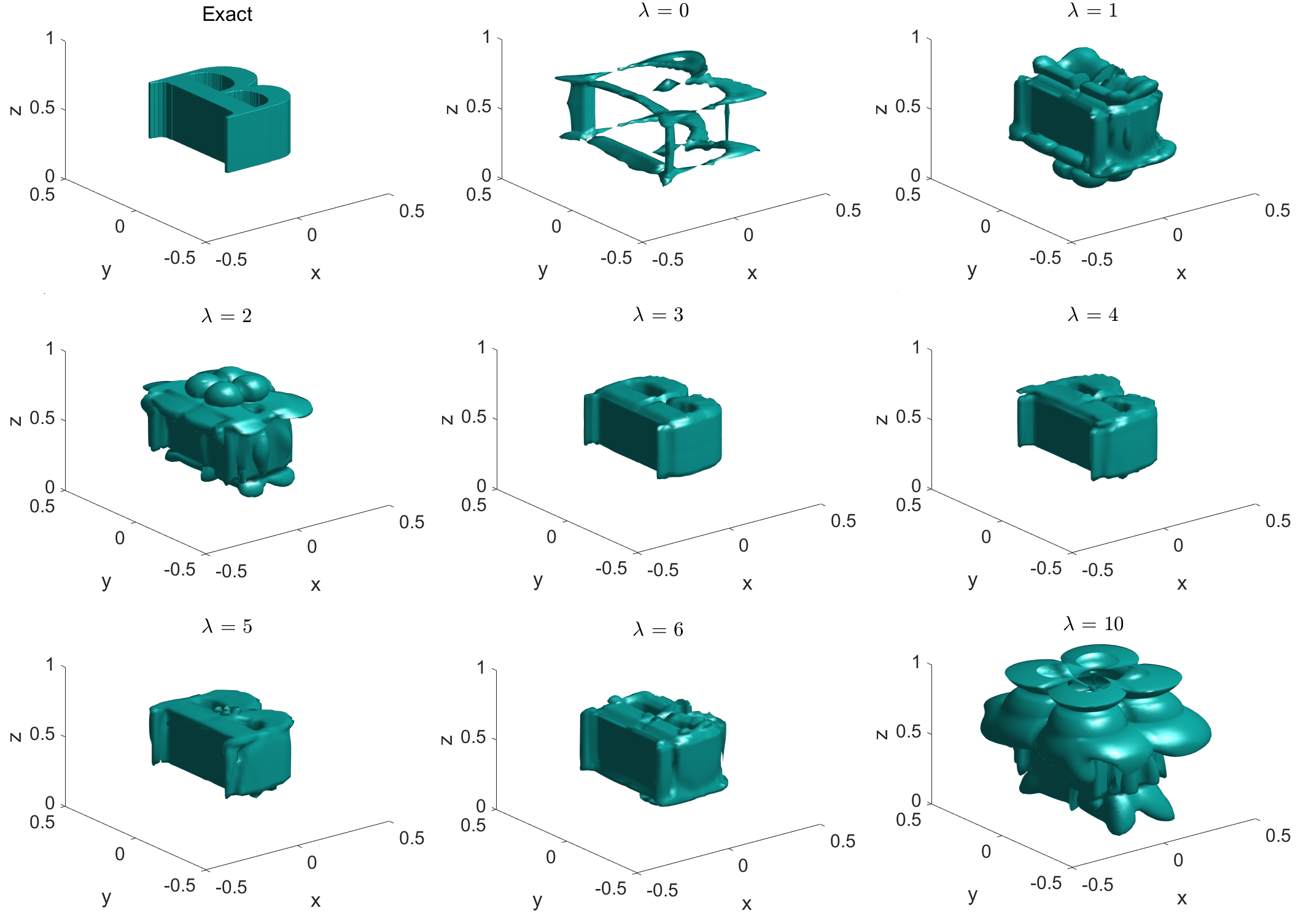
Figure 2: Test 1: The reconstructions of $n(\mathbf{x})$ of different $\lambda$ with $N=8$, when the shape of the inclusion in (67) is horizontal letter ‘$B$’ with $c_{a}=1.5$. The value of $\lambda$ can be seen on the top side of each square. The images have a low quality for $\lambda=0,1,2$. The quality is improved with $\lambda=3,4,5$. Then it starts to deteriorate at $\lambda=6$ and becomes unsatisfactory at $\lambda=10$. Thus, we select $\lambda=3$ as the optimal value of the parameter $\lambda$.

Next, we fix the optimal value of $\lambda=3$ and test the influence of the parameter $N$. The results with $N=2,4,8$ are shown in Figure 3. We can find that the reconstruction for $N=2$ is of a low quality, and the reconstructions for $N=4,8$ are almost same. Hence, to reduce the computational cost we select $N=4$ as the optimal value of $N$, instead of $N=8$. Furthermore, we also consider the truncated expansion of the function $u\left(r,\varphi,z,z_{0}\right)$ in (26) with $N=4$, which is denoted as $u_{4}\left(r,\varphi,z,z_{0}\right)$. We have obtained that

(74) $$\frac{\left\|u_{4}\left(r,\varphi,z,z_{0}\right)\right\|_{L_{2}\left(\Omega\times\left(0,B\right)\right)}}{\left\|u\left(r,\varphi,z,z_{0}\right)\right\|_{L_{2}\left(\Omega\times\left(0,B\right)\right)}}=99.86\%.$$

It is clear from (74) that $N=4$ is a quite informative case.

Conclusion: We choose

(75) $$\lambda=3,N=4$$

as the optimal values of these parameters, and we use these values in Tests 2-5.

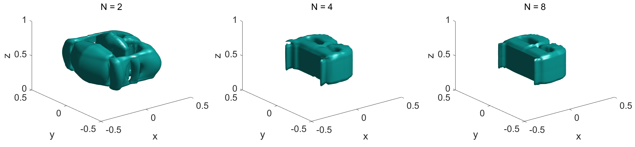
Figure 3: Test 1: Reconstructions of $n(\mathbf{x})$ of $N=2,4,8$ at $\lambda=3$, when the shape of the inclusion in (67) is horizontal letter ‘$B$’ with $c_{a}=1.5$. The reconstruction for $N=2$ has a low quality, and the reconstructions for $N=4,8$ are almost same. Thus, keeping also in mind (74) and (75) and also to reduce the computational cost, we choose in Tests 2-5 $N=4$ and $\lambda=3$.

Test 2. We test the case when the inclusion in (67) has the shape of the vertically oriented letter ‘$B$’ with $c_{a}=1.5$ in it. Results are presented on Figure 4. An accurate reconstruction can be observed.

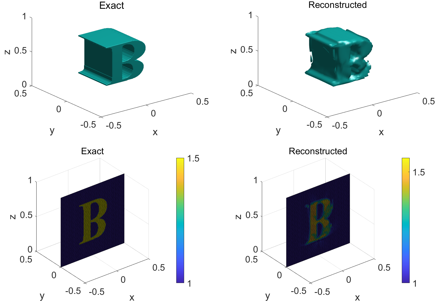
Figure 4: Test 2: The exact (left) and reconstructed (right) function $n(\mathbf{x})$, when the shape of the inclusion in (67) is vertically oriented letter ‘$B$’ with $c_{a}=1.5$ in it. Here $\lambda=3,N=4$ as in (75). The reconstruction is accurate.

Test 3. We test the cases when the inclusion in (67) has the shape of the vertically oriented letter ‘$B$’ with $c_{a}=3$ and $c_{a}=5$ in it. Results are displayed on Figures 5 and 6 respectively. The inclusion/background contrasts in (68) are respectively $3:1$ and $5:1$. We see that shape of the inclusion is imaged accurately in both cases. In addition, the computed inclusion/background contrasts in (69) are accurate.

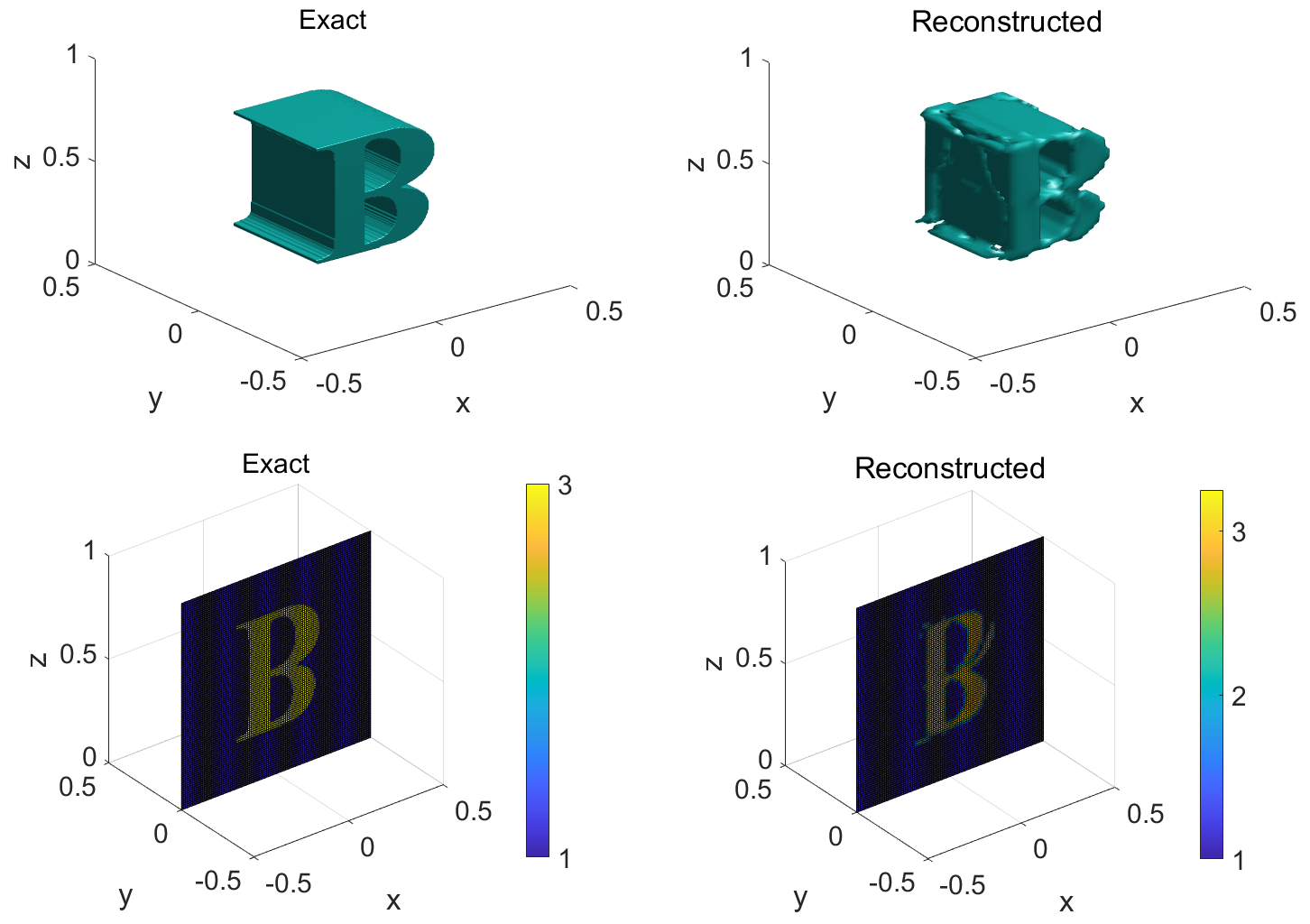
Figure 5: Test 3: The exact (left) and reconstructed (right) function $n(\mathbf{x})$, when the shape of the inclusion in (67) is vertically oriented letter ‘$B$’ with $c_{a}=3$ in it. Here $\lambda=3,N=4$ as in (75). The inclusion/background contrast in (68) is $3:1$. The computed inclusion/background contrast in (69) is accurate.

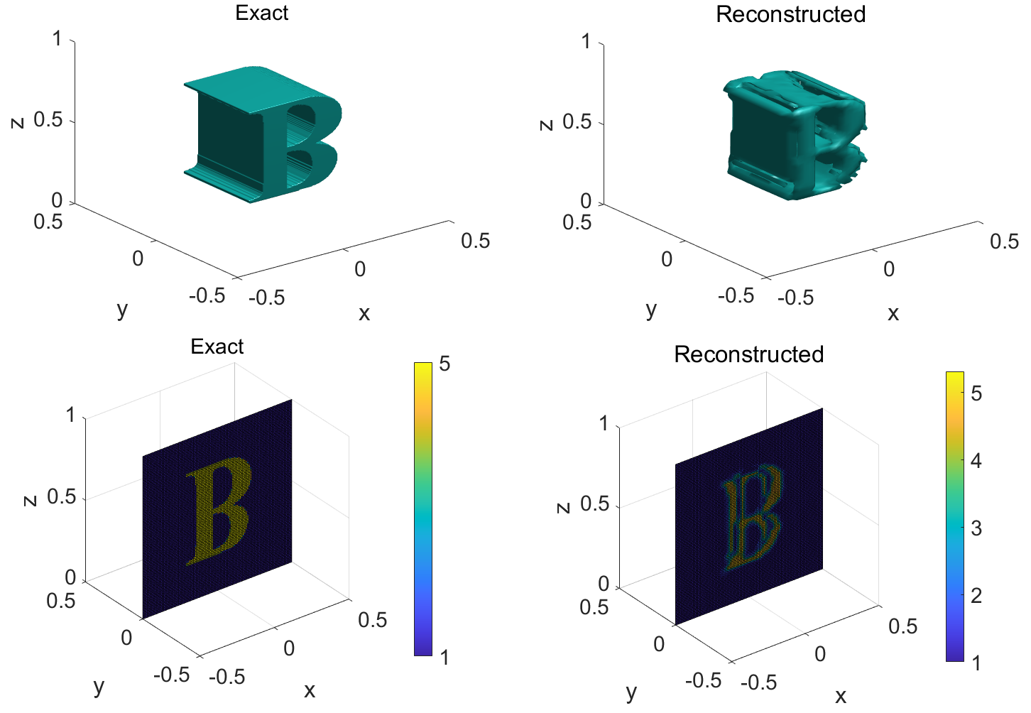
Figure 6: Test 3: The exact (left) and reconstructed (right) function $n(\mathbf{x})$, when the shape of the inclusion in (67) is vertically oriented letter ‘$B$’ with $c_{a}=5$ in it. Here $\lambda=3,N=4$ as in (75). The inclusion/background contrast in ( 68) is $5:1$. The computed inclusion/background contrast in ( 69) is accurate.

Test 4. We test the case when the inclusion in (67) has the shape of the letter ‘$O$’ elongated along the $y-$axis and with $c_{a}=1.5$ in it. Results are presented on Figure 7. We again observe an accurate reconstruction of both the shape of the inclusion and the inclusion/background contrast.

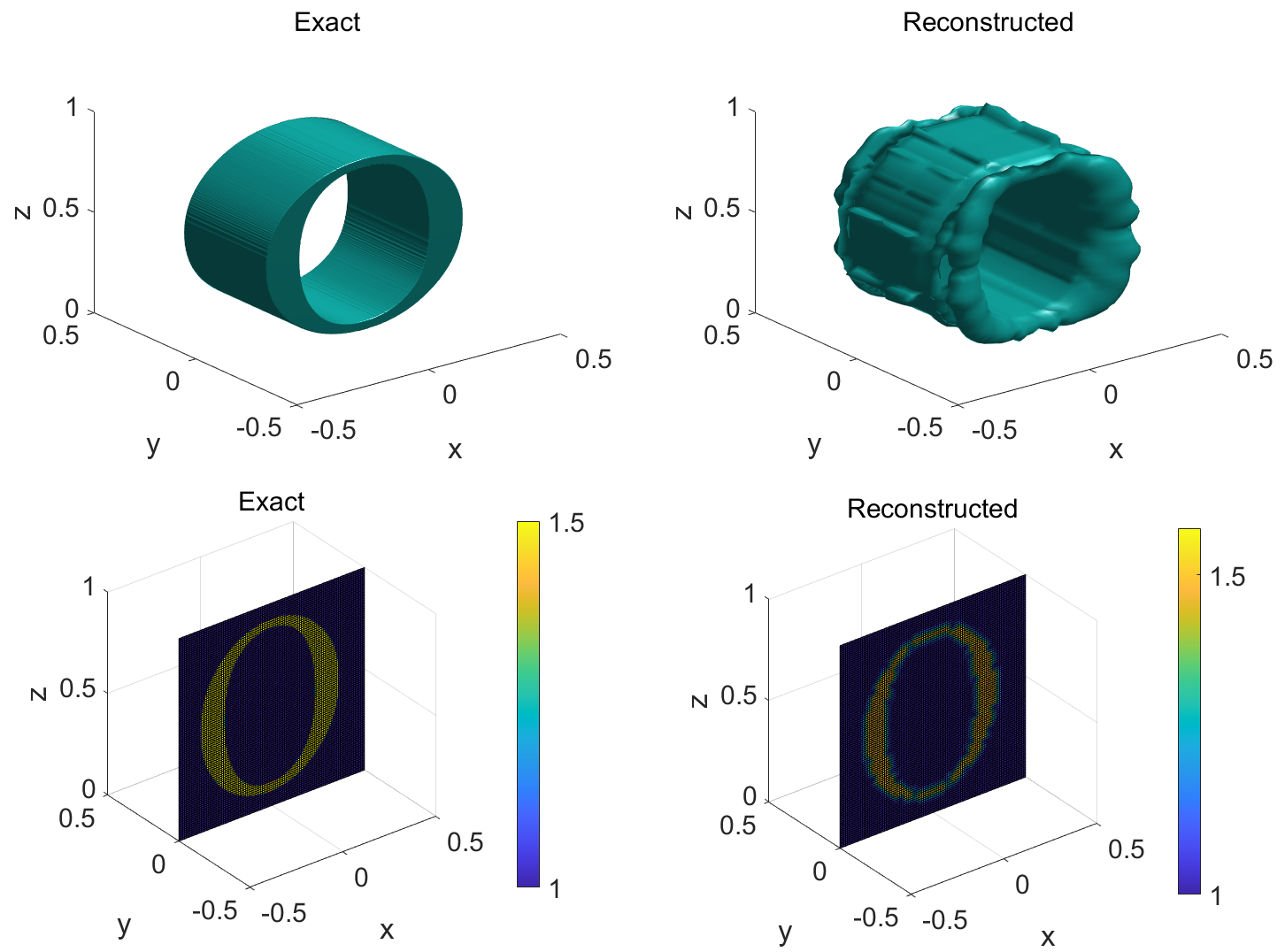
Figure 7: Test 4: The exact (left) and reconstructed (right) function $n(\mathbf{x})$, when the shape of the inclusion in (67) is the letter ‘$O$’ elongated along the y-axis and with $c_{a}=1.5$ in it. Here $\lambda=3,N=4$ as in (75). The reconstruction is accurate.

Test 5. We consider the case when the random noise is present in the data in (71)-(73) with $\delta=0.01$ and $\delta=0.03$, i.e. with 1% and 3% noise level respectively. We test the reconstruction for the case when the inclusion in (67) has the shape of the vertically oriented letter ‘$B$’ with $c_{a}=1.5$ in it. Results are displayed on Figure 8. The reconstructions of the shape of the inclusion as well as computed inclusion/background contrasts in (69) are accurate.

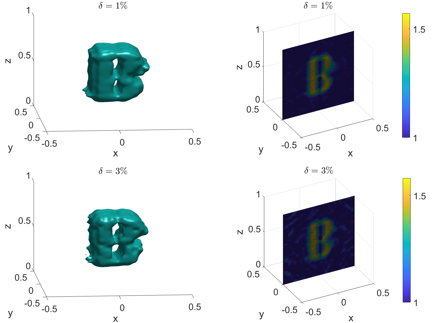
Figure 8: Test 5: Reconstructed function $n(\mathbf{x})$ with $\sigma=0.01$ (top) and $\sigma=0.03$ (bottom), i.e. with 1% and 3% noise level, when the shape of the inclusion in (67) is vertically oriented letter ‘$B$’ with $c_{a}=1.5$ in it. Here $\lambda=3,N=4$ as in (75). The reconstructions and computed inclusion/background contrasts in (69) are accurate.

Remarks 9.1:

1. Recall that by Theorem 3.1 condition (11) is a sufficient condition for our method to work. Recall also that in the data generation process we smooth out tested inclusions in small neighborhoods of their boundaries. Given these, a careful analysis of correct images of Figures 2-8 indicates that condition (11) is satisfied at least in a major part of the domain $\Omega$ in each of the above Tests 1-5.

2. We conclude, therefore, that our method works numerically under conditions which are broader than (11). In other words, (11) is not a necessary condition for our method to work. Establishing necessary conditions is outside of the scope of the current publication.

Acknowledgments. The work of Li was partially supported by Guangdong Basic and Applied Basic Research Foundation 2023B1515250005. The work of Romanov was partially supported by the Mathematical Center in Akademgorodok under Agreement 075152022281 with the Ministry of Science and Higher Education of the Russian Federation. The work of Yang was partially supported by Supercomputing Center of Lanzhou University.

References

- [1] L. Baudouin, M. de Buhan, and S. Ervedoza, Convergent algorithm based on Carleman estimates for the recovery of a potential in the wave equation, SIAM J. Numer. Anal., 55 (2017), pp. 1578–1613.
- [2] L. Baudouin, M. de Buhan, S. Ervedoza, and A. Osses, Carleman-based reconstruction algorithm for the waves, SIAM J. Numer. Anal., 59 (2021), pp. 998–1039.
- [3] L. Beilina and E. Lindström, An adaptive finite element/finite difference domain decomposition method for applications in microwave imaging, Electronics, 11 (2022), p. 1359.
- [4] A. V. Goncharsky, S. Y. Romanov, and S. Y. Seryozhnikov, On mathematical problems of two-coefficient inverse problems of ultrasonic tomography, Inverse Probl., 40 (2024), p. 045026.
- [5] M. J. Grote and U. Nahum, Adaptive eigenspace for multi-parameter inverse scattering problems, Computers & Mathematics with Applications, 77 (2019), pp. 3264–3280.
- [6] J. P. Guillement and R. G. Novikov, Inversion of weighted Radon transforms via finite Fourier series weight approximation, Inverse Probl. Sci. En., 22 (2013), pp. 787–802.
- [7] G. Herglotz, Űber die Elastizitaet der Erde bei Beruecksichtigung ihrer variablen Dichte, Zeitschr. fur Math. Phys., 52 (1905), pp. 275–299.
- [8] S. I. Kabanikhin, K. K. Sabelfeld, N. S. Novikov, and M. A. Shishlenin, Numerical solution of the multidimensional Gelfand-Levitan equation, J. Inverse Ill-Posed Probl., 23 (2015), pp. 439–450.
- [9] M. V. Klibanov and O. V. Ioussoupova, Uniform strict convexity of a cost functional for three-dimensional inverse scattering problem, SIAM J. Math. Anal, 26 (1995), pp. 147–179.
- [10] M. V. Klibanov, Global convexity in a three-dimensional inverse acoustic problem, SIAM J. Math. Anal., 28 (1997), pp. 1371–1388.
- [11] M. V. Klibanov, Convexification of restricted Dirichlet to Neumann map, J. Inverse Ill-Posed Probl., 25 (2017), pp. 669–685.
- [12] M. V. Klibanov, Travel time tomography with formally determined incomplete data in 3D, Inverse Problems and Imaging, 13 (2019), pp. 1367–1393.
- [13] M. V. Klibanov, J. Li, and W. Zhang, Convexification for an inverse parabolic problem, Inverse Probl., 36 (2020), p. 085008.
- [14] M. V. Klibanov and J. Li, Inverse Problems and Carleman Estimates: Global Uniqueness, Global Convergence and Experimental Data, De Gruyter, Berlin, 2021.
- [15] M. V. Klibanov, J. Li, and W. Zhang, Numerical solution of the 3-D travel time tomography problem, J. Computational Physics, 476 (2023), p. 111910.
- [16] M. V. Klibanov, J. Li, and Z. Yang, Convexification numerical method for the retrospective problem of mean field games, Applied Mathematics and Optimization, (2024), 90:6.
- [17] R. G. Mukhometov, The reconstruction problem of a two-dimensional Riemannian metric and integral geometry, Soviet Math. Dokl., 18 (1977), pp. 32–35.
- [18] R. G. Mukhometov and V. G. Romanov, On the problem of determining an isotropic Riemannian metric in the -dimensional space, Dokl. Acad. Sci. USSR, 19 (1978), pp. 1330–1333.
- [19] L. Pestov and G. Uhlmann, Two dimensional simple Riemannian manifolds are boundary distance rigid, Annals of Mathematics, 161 (2005), pp. 1093–1110.
- [20] G. Peyre, Toolbox fast marching, MATLAB Central File Exchange, (2023).
- [21] V. G. Romanov, Inverse Problems of Mathematical Physics, VNU Press, Utrecht, The Netherlands, 1986.
- [22] U. Schrőder and T. Schuster, An iterative method to reconstruct the refractive index of a medium from time-off-light measurements, Inverse Problems, 32 (2016), p. 085009.
- [23] A. N. Tikhonov, A. V. Goncharsky, V. V. Stepanov, and A. G. Yagola, Numerical methods for the solution of Ill-posed problems, Kluwer, London, 1995.
- [24] L. Volgyesi and M. Moser, The inner structure of the Earth, Periodica Polytechnica Chemical Engineering, 26 (1982), pp. 155–204.
- [25] E. Wiechert and K. Zoeppritz, Uber Erdbebenwellen, Nachr. Koenigl. Geselschaft Wiss. Gottingen, (1907), pp. 415–549.
- [26] H. Zhao and Y. Zhong, A hybrid adaptive phase space method for reflection traveltime tomography, SIAM J. Imaging Sciences, 12 (2019), pp. 28–53.