Test Time Learning for Time Series Forecasting

Abstract

Time-series forecasting has seen significant advancements with the introduction of token prediction mechanisms such as multi-head attention. However, these methods often struggle to achieve the same performance as in language modeling, primarily due to the quadratic computational cost and the complexity of capturing long-range dependencies in time-series data. State-space models (SSMs), such as Mamba, have shown promise in addressing these challenges by offering efficient solutions with linear RNNs capable of modeling long sequences with larger context windows. However, there remains room for improvement in accuracy and scalability.

We propose the use of Test-Time Training (TTT) modules in a parallel architecture to enhance performance in long-term time series forecasting. Through extensive experiments on standard benchmark datasets, we demonstrate that TTT modules consistently outperform state-of-the-art models, including the Mamba-based TimeMachine, particularly in scenarios involving extended sequence and prediction lengths. Our results show significant improvements in Mean Squared Error (MSE) and Mean Absolute Error (MAE), especially on larger datasets such as Electricity, Traffic, and Weather, underscoring the effectiveness of TTT in capturing long-range dependencies. Additionally, we explore various convolutional architectures within the TTT framework, showing that even simple configurations like 1D convolution with small filters can achieve competitive results. This work sets a new benchmark for time-series forecasting and lays the groundwork for future research in scalable, high-performance forecasting models.

Keywords Time Series Forecasting  $\cdot$ Test-Time Training  $\cdot$ Mamba  $\cdot$ Expressive Hidden States

1 Introduction

Long Time Series Forecasting (LTSF) is a crucial task in various fields, including energy, industry, defense, and atmospheric sciences. LTSF uses a historical sequence of observations, known as the look-back window, to predict future values through a learned or mathematically induced model. However, the stochastic nature of real-world events makes LTSF challenging. Deep learning models, including time series forecasting, have been widely adopted in engineering and scientific fields. Early approaches employed Recurrent Neural Networks (RNNs) to capture long-range dependencies in sequential data like time series. However, recurrent architectures like RNNs have limited memory retention, are difficult to parallelize, and have constrained expressive capacity. Transformers [25], with ability to efficiently process sequential data in parallel and capture contextual information, have significantly improved performance on time series prediction task [26, 16, 20, 3]. Yet, due to the quadratic complexity of attention mechanisms with respect to the context window (or look-back window in LTSF), Transformers are limited in their ability to capture very long dependencies.

In recent years, State Space Models (SSMs) such as Mamba  [7], a gated linear RNN variant, have revitalized the use of RNNs for LTSF. These models efficiently capture much longer dependencies while reducing computational costs and enhancing expressive power and memory retention. A new class of Linear RNNs, known as Test Time Training (TTT) modules  [24], has emerged. These modules use expressive hidden states and provide theoretical guarantees for capturing long-range dependencies, positioning them as one of the most promising architectures for LTSF.

Key Insights and Results

Through our experiments, several key insights emerged regarding the performance of TTT modules when compared to existing SOTA models:

• Superior Performance with Longer Sequence and Prediction Lengths: TTT modules consistently outperformed the SOTA TimeMachine model, particularly as sequence and prediction lengths increased. Architectures such as Conv Stack 5 demonstrated their ability to capture long-range dependencies more effectively than Mamba-based models, resulting in noticeable improvements in Mean Squared Error (MSE) and Mean Absolute Error (MAE) across various benchmark datasets.

• Strong Improvement on Larger Datasets: On larger datasets, such as Electricity, Traffic, and Weather, the TTT-based models excelled, showing superior performance compared to both Transformer- and Mamba-based models. These results underscore the ability of TTT to handle larger temporal windows and more complex data, making it especially effective in high-dimensional, multivariate datasets.

• Hidden Layer Architectures: The ablation studies revealed that while convolutional architectures added to the TTT modules provided some improvements, Conv Stack 5 consistently delivered the best results among the convolutional variants. However, simpler architectures like Conv 3 often performed comparably, showing that increased architectural complexity did not always lead to significantly better performance. Very complex architectures like the modern convolutional block from [5] showed competitive performance when used as TTT hidden layer architectures compared to the simpler single architectures proposed, hinting on the potential of more complex architectures in capturing more long term dependencies.

• Adaptability to Long-Term Predictions: The TTT-based models excelled in long-term prediction tasks, especially for really high prediction lengths like 2880. TTT-based models also excelled on increased sequence lengths as high as 5760 which is the maximum sequence length allowed by the benchmark datasets. This verified the theoretically expected superiority of TTT based models relative to the mamba/transformer based SOTA models.

Motivation and Contributions

In this work, we explore the potential of TTT modules in Long-Term Series Forecasting (LTSF) by integrating them into novel model configurations to surpass the current state-of-the-art (SOTA) models. Our key contributions are as follows:

• We propose a new model architecture utilizing quadruple TTT modules, inspired by the TimeMachine model  [1], which currently holds SOTA performance. By replacing the Mamba modules with TTT modules, our model effectively captures longer dependencies and predicts larger sequences.

• We evaluate the model on benchmark datasets, exploring the original look-back window and prediction lengths to identify the limitations of the SOTA architecture. We demonstrate that the SOTA model achieves its performance primarily by constraining look-back windows and prediction lengths, thereby not fully leveraging the potential of LTSF.

• We extend our evaluations to significantly larger sequence and prediction lengths, showing that our TTT-based model consistently outperforms the SOTA model using Mamba modules, particularly in scenarios involving extended look-back windows and long-range predictions.

• We conduct an ablation study to assess the performance of various hidden layer architectures within our model. By testing six different convolutional configurations, one of which being ModernTCN by [5], we quantify their impact on model performance and provide insights into how they compare with the SOTA model.

2 Related Work

Transformers for LTSF

Several Transformer-based models have advanced long-term time series forecasting (LTSF), with notable examples like iTransformer [18] and PatchTST
 [21]. iTransformer employs multimodal interactive attention to capture both temporal and inter-modal dependencies, suitable for multivariate time series, though it incurs high computational costs when multimodal data interactions are minimal. PatchTST, inspired by Vision Transformers [6], splits input sequences into patches to capture dependencies effectively, but its performance hinges on selecting the appropriate patch size and may reduce model interpretability. Other influential models include Informer [31], which uses sparse self-attention to reduce complexity but may overlook finer details in multivariate data; Autoformer [28], which excels in periodic data but struggles with non-periodic patterns; Pyraformer [16], which captures multi-scale dependencies through a hierarchical structure but at the cost of increased computational requirements; and Fedformer [32], which combines time- and frequency-domain representations for efficiency but may underperform on noisy time series. While each model advances LTSF in unique ways, they also introduce specific trade-offs and limitations.

State Space Models for LTSF

S4 models [8, 9, 10] are efficient sequence models for long-term time series forecasting (LTSF), leveraging linear complexity through four key components: $\Delta$ (discretization step size), $A$ (state update matrix), $B$ (input matrix), and $C$ (output matrix). They operate in linear recurrence for autoregressive inference and global convolution for parallel training, efficiently transforming recurrences into convolutions. However, S4 struggles with time-invariance issues, limiting selective memory. Mamba [7] addresses this by making $B$, $C$, and $\Delta$ dynamic, creating adaptable parameters that improve noise filtering and maintain Transformer-level performance with linear complexity. SIMBA [23] enhances S4 by integrating block-sparse attention, blending state space and attention to efficiently capture long-range dependencies while reducing computational overhead, ideal for large-scale, noisy data. TimeMachine [1] builds on these advances by employing a quadruple Mamba setup, managing both channel mixing and independence while avoiding Transformers’ quadratic complexity through multi-scale context generation, thereby maintaining high performance in long-term forecasting tasks.

Linear RNNs for LTSF

RWKV-TS [11] is a novel linear RNN architecture designed for time series tasks, achieving O(L) time and memory complexity with improved long-range information capture, making it more efficient and scalable compared to traditional RNNs like LSTM and GRU. [22] introduced the Linear Recurrent Unit (LRU), an RNN block matching the performance of S4 models on long-range reasoning tasks while maintaining computational efficiency. TTT [24] layers take a novel approach by treating the hidden state as a trainable model, learning during both training and test time with dynamically updated weights. This allows TTT to capture long-term relationships more effectively through real-time updates, providing an efficient, parallelizable alternative to self-attention with linear complexity. TTT’s adaptability and efficiency make it a strong candidate for processing longer contexts, addressing the scalability challenges of RNNs and outperforming Transformer-based architectures in this regard.

MLPs and CNNs for LTSF

Recent advancements in long-term time series forecasting (LTSF) have introduced efficient architectures that avoid the complexity of attention mechanisms and recurrence. TSMixer [2], an MLP-based model, achieves competitive performance by separating temporal and feature interactions through time- and channel-mixing, enabling linear scaling with sequence length. However, MLPs may struggle with long-range dependencies and require careful hyperparameter tuning, especially for smaller datasets. Convolutional neural networks (CNNs) have also proven effective for LTSF, particularly in capturing local temporal patterns. ModernTCN [5] improves temporal convolution networks (TCNs) using dilated convolutions and a hierarchical structure to efficiently capture both short- and long-range dependencies, making it well-suited for multi-scale time series data.

Building on these developments, we improve the original TimeMachine model by replacing its Mamba blocks with Test-Time Training (TTT) blocks to enhance long-context prediction capabilities. We also explore CNN configurations, such as convolutional stacks, to enrich local temporal feature extraction. This hybrid approach combines the efficiency of MLPs, the local pattern recognition of CNNs, and the global context modeling of TTT, leading to a more robust architecture for LTSF tasks that balances both short- and long-term forecasting needs.

3 Model Architecture

The task of Time Series Forecasting can be defined as follows: Given a multivariate time series dataset with a window of past observations (look-back window) $L$: $(\mathbf{x}_{1},\dots,\mathbf{x}_{L})$, where each $\mathbf{x}t$ is a vector of dimension $M$ (the number of channels at time $t$), the goal is to predict the next $T$ future values $(\mathbf{x}_{L+1},\dots,\mathbf{x}_{L+T})$.

The TimeMachine [1] architecture, which we used as the backbone, is designed to capture long-term dependencies in multivariate time series data, offering linear scalability and a small memory footprint. It integrates four Mamba [7] modules as sequence modeling blocks to selectively memorize or forget historical data, and employs two levels of downsampling to generate contextual cues at both high and low resolutions.

However, Mamba’s approach still relies on fixed-size hidden states to compress historical information over time, often leading to the model forgetting earlier information in long sequences. TTT [24] uses dynamically updated weights (in the form of matrices inside linear or MLP layers) to compress and store historical data. This dynamic adjustment during test time allows TTT to better capture long-term relationships by continuously incorporating new information. Its Hidden State Updating Rule is defined as:

$$W_{t}=W_{t-1}-\eta\nabla\ell(W_{t-1};x_{t})=W_{t-1}-\eta\nabla\|f(\tilde{x}_{t};W)-x_{t}\|^{2}$$

We incorporated TTT into the TimeMachine model, replacing the original Mamba block. We evaluated our approach with various setups, including different backbones and TTT layer configurations. Additionally, we introduced convolutional layers before the sequence modeling block and conducted experiments with different context lengths and prediction lengths.

Our goal is to improve upon the performance of the state-of-the-art (SOTA) models in LTSF using the latest advancements in sequential modeling. Specifically, we integrate Test-Time Training (TTT) modules into our model for two key reasons, TTT is theoretically proven to have an extremely long context window, being a form of linear RNN [22], capable of capturing long-range dependencies efficiently. Secondly, the expressive hidden states of TTT allow the model to capture a diverse set of features without being constrained by the architecture, including the depth of the hidden layers, their size, or the types of blocks used.

3.1 General Architecture

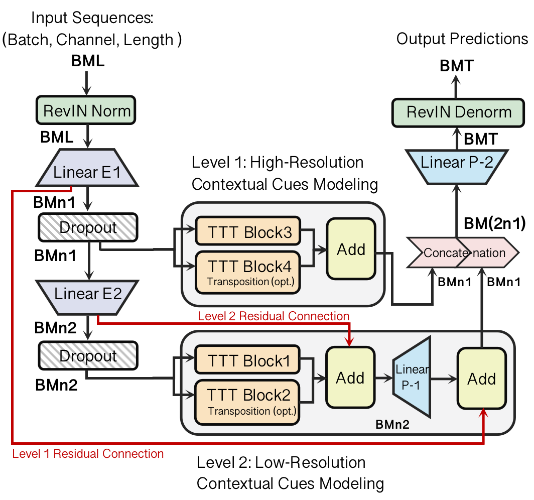
(a) TimeMachine incoporating TTT-Blocks

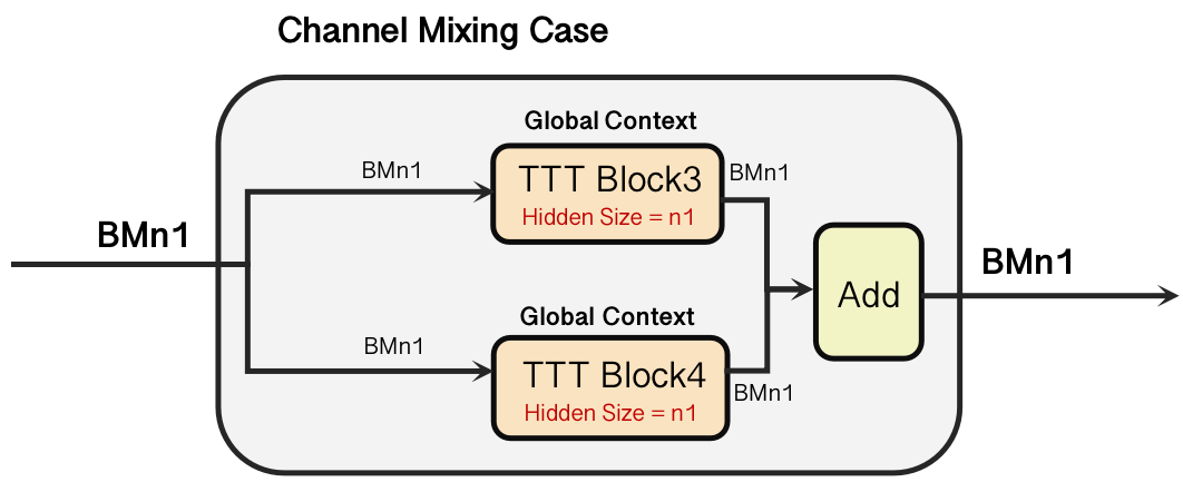
(b) Channel Mixing Mode

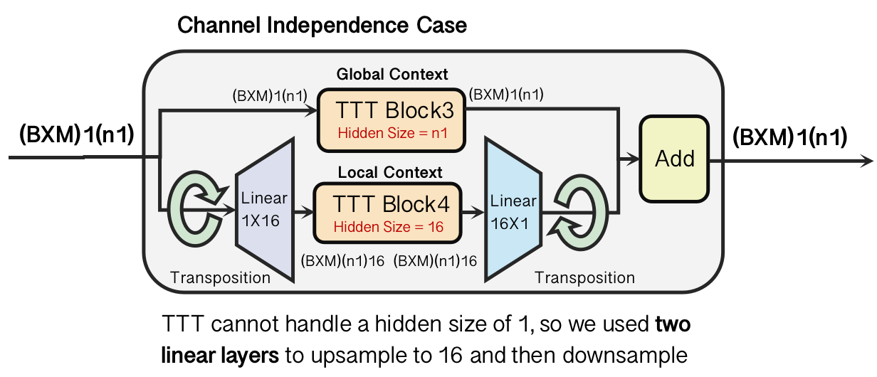
(c) Channel Independence Mode

Figure 1: Our model architecture. (a) We replace the four Mamba Block in TimeMachine with four TTT(Test-Time Training) Block. (b) There are two modes of TimeMachine, the channel mixing mode for capturing strong between-channel correlations, and the channel independence mode for modeling within-channel dynamics. Recent works such as PatchTST  [21] and TiDE  [4] have shown channel independence can achieve SOTA accuracy. For the channel independence scenario, the inputs are first transposed, and then we integrate two linear layers ($1\times 16$ and $16\times 1$) to provide the TTT Block with a sufficiently large hidden size.

Our model architecture builds upon the TimeMachine model [1], introducing key modifications, as shown in Figure 1, 1 and 1. Specifically, we replace the Mamba modules in TimeMachine with TTT (Test-Time Training) modules [24], which retain compatibility since both are linear RNNs [22]. However, TTT offers superior long-range dependency modeling due to its adaptive nature and theoretically infinite context window. A detailed visualization of the TTT block and the different proposed architectures can be found in Appendix B

Our model features a two-level hierarchical architecture that captures both high-resolution and low-resolution context, as illustrated in Figure 1. To adapts to the specific characteristics of the dataset, the architecture handles two scenarios—Channel Mixing and Channel Independence—illustrated in Figure 1 and 1 respectively. A more detailed and mathematical description of the normalization and prediction procedures can be found in Appendix B.

3.2 Hierarchical Embedding

The input sequence $BML$ (Batch, Channel, Length) is first passed through Reversible Instance Normalization [12] (RevIN), which stabilizes the model by normalizing the input data and helps mitigate distribution shifts. This operation is essential for improving generalization across datasets.

After normalization, the sequence passes through two linear embedding layers. Linear E1 and Linear E2 are used to map the input sequence into two embedding levels: higher resolution and lower resolution. The embedding operations $E_{1}:\mathbb{R}^{M\times L}\rightarrow\mathbb{R}^{M\times n_{1}}$ and $E_{2}:\mathbb{R}^{M\times n_{1}}\rightarrow\mathbb{R}^{M\times n_{2}}$ are achieved through MLP. $n_{1}$ and $n_{2}$ are configurations that take values from $\{512,256,128,64,32\}$, satisfying $n_{1}>n_{2}$. Dropout layers are applied after each embedding layer to prevent overfitting, especially for long-term time series data. As shown in Figure 1.

3.3 Two Level Contextual Cue Modeling

At each of the two embedding levels, a contextual cues modeling block processes the output from the Dropout layer following E1 and E2. This hierarchical architecture captures both fine-grained and broad temporal patterns, leading to improved forecasting accuracy for long-term time series data.

In Level 1, High-Resolution Contextual Cues Modeling is responsible for modeling high-resolution contextual cues. TTT Block 3 and TTT Block 4 process the input tensor, focusing on capturing fine-grained temporal dependencies. The TTT Block3 operates directly on the input, and transposition may be applied before TTT Block4 if necessary. The outputs are summed, then concatenated with the Level 2 output. There is no residual connection summing in Level 1 modeling.

In Level 2, Low-Resolution Contextual Cues Modeling handles broader temporal patterns, functioning similarly to Level 1. TTT Block 1 and TTT Block 2 process the input tensor to capture low-resolution temporal cues and add them togther. A linear projection layer (P-1) is then applied to maps the output (with dimension RM×n2) to a higher dimension RM×n1, preparing it for concatenation. Additionally, the Level 1 and Level 2 Residual Connections ensure that information from previous layers is effectively preserved and passed on.

3.4 Final Prediction

After processing both high-resolution and low-resolution cues, the model concatenates the outputs from both levels. A final linear projection layer (P-2) is then applied to generate the output predictions. The output is subsequently passed through RevIN Denormalization, which reverses the initial normalization and maps the output back to its original scale for interpretability. For more detailed explanations and mathematical descriptions refer to Appendix B.

3.5 Channel Mixing and Independence Modes

The Channel Mixing Mode (Figure 1 and 1) processes all channels of a multivariate time series together, allowing the model to capture potential correlations between different channels and understand their interactions over longer time. Figure 1 illustrates an example of the channel mixing case, but there is also a channel independence case corresponding to Figure 1, which we have not shown here. Figures 1 and 1 demonstrate the channel mixing and independence modes of the Level 1 High-Resolution Contextual Cues Modeling part with TTT Block 3 and TTT Block 4. Similar versions of the two channel modes for Level 2 Low-Resolution Contextual Cues Modeling are quite similar to those in Level 1, which we have also omitted here.

The Channel Independence Mode (Figure 1) treats each channel of a multivariate time series as an independent sequence, enabling the model to analyze individual time series more accurately. This mode focuses on learning patterns within each channel without considering potential correlations between them.

The main difference between these two modes is that the Channel Independence Mode always uses transposition before and after one of the TTT blocks (in Figure 1, it’s TTT Block 4). This allows the block to capture contextual cues from local perspectives, while the other block focuses on modeling the global context. However, in the Channel Mixing Mode, both TTT Block 3 and TTT Block 4 model the global context.

The hidden size value for TTT Blocks in global context modeling is set to $n_{1}$ since the input shape is $BMn_{1}$ for Channel Mixing and $(B\times M)1{n_{1}}$ for Channel Independence. To make the TTT Block compatible with the local context modeling scenario—where the input becomes $(B\times M){n_{1}}\leftarrow\text{Transpose}((B\times M)1{n_{1}})$ after transposition—we add two linear layers: one for upsampling to $(B\times M){n_{1}}16$ and another for downsampling back. In this case, the hidden size of TTT Block 4 is set to 16.

4 Experiments and Evaluation

4.1 Original Experimental Setup

We evaluate our model on seven benchmark datasets that are commonly used for LTSF, namely: Traffic, Weather, Electricity, ETTh1, ETTh2, ETTm1, and ETTm2 from  [28] and  [31]. Among these, the Traffic and Electricity datasets are significantly larger, with 862 and 321 channels, respectively, and each containing tens of thousands of temporal points. Table 6 summarizes the dataset details in Appendix D.

For all experiments, we adopted the same setup as in [18], fixing the look-back window $L=96$ and testing four different prediction lengths $T={96,192,336,720}$. We compared our TimeMachine-TTT model against 12 state-of-the-art (SOTA) models, including TimeMachine  [1], iTransformer  [18], PatchTST  [21], DLinear  [29], RLinear  [14], Autoformer  [28], Crossformer  [30], TiDE  [4], Scinet  [15], TimesNet  [27], FEDformer  [32], and Stationary  [19]. All experiments were conducted with both MLP and Linear architectures using the original Mamba backbone, and we confirmed the results from the TimeMachine paper.

4.2 Quantitative Results

Across all seven benchmark datasets, our TimeMachine-TTT model consistently demonstrated superior performance compared to SOTA models. In the Weather dataset, TTT achieved leading performance at longer horizons (336 and 720), with MSEs of 0.248 and 0.341, respectively, outperforming TimeMachine, which recorded MSEs of 0.256 and 0.342. The Traffic dataset, with its high number of channels (862), also saw TTT outperform TimeMachine and iTransformer at both short (96-step MSE of 0.394 vs. 0.397) and long horizons (720-step MSE of 0.464 vs. 0.467), highlighting the model’s ability to handle multivariate time series data.

Table 1: Results in MSE and MAE (the lower the better) for the long-term forecasting task. We compare extensively with baselines under different prediction lengths, $T=\{96,192,336,720\}$ following the setting of iTransformer [17]. The length of the input sequence ($L$) is set to 96 for all baselines. TTT (ours) is our TTT block with the Conv Stack 5 architecture. The best results are in bold and the second best are underlined.

Methods$\rightarrow$		TTT(ours)		TimeMachine		iTransformer		RLinear		PatchTST		Crossformer		TiDE		TimesNet		DLinear		SCINet		FEDformer		Stationary
$\mathcal{D}$	$T$	MSE	MAE	MSE	MAE	MSE	MAE	MSE	MAE	MSE	MAE	MSE	MAE	MSE	MAE	MSE	MAE	MSE	MAE	MSE	MAE	MSE	MAE	MSE	MAE
Weather	96	0.163	0.211	0.164	0.208	0.174	0.214	0.192	0.232	0.177	0.218	0.158	0.230	0.202	0.261	0.172	0.220	0.196	0.255	0.221	0.306	0.217	0.296	0.173	0.223
	192	0.220	0.258	0.211	0.250	0.221	0.254	0.240	0.271	0.225	0.259	0.206	0.277	0.242	0.298	0.219	0.261	0.237	0.296	0.261	0.340	0.276	0.336	0.245	0.285
	336	0.248	0.279	0.256	0.290	0.278	0.296	0.292	0.307	0.278	0.297	0.272	0.335	0.287	0.335	0.280	0.306	0.283	0.335	0.309	0.378	0.339	0.380	0.321	0.338
	720	0.341	0.342	0.342	0.343	0.358	0.349	0.364	0.353	0.354	0.348	0.398	0.418	0.351	0.386	0.365	0.359	0.345	0.381	0.377	0.427	0.403	0.428	0.414	0.410
Traffic	96	0.394	0.264	0.397	0.268	0.395	0.268	0.649	0.389	0.544	0.359	0.522	0.290	0.805	0.493	0.593	0.321	0.650	0.396	0.788	0.499	0.587	0.366	0.612	0.338
	192	0.441	0.292	0.417	0.274	0.417	0.276	0.601	0.366	0.540	0.354	0.530	0.293	0.756	0.474	0.617	0.336	0.598	0.370	0.789	0.505	0.604	0.373	0.613	0.340
	336	0.433	0.281	0.433	0.281	0.433	0.283	0.609	0.369	0.551	0.358	0.558	0.305	0.762	0.477	0.629	0.336	0.605	0.373	0.797	0.508	0.621	0.383	0.618	0.328
	720	0.464	0.293	0.467	0.300	0.467	0.302	0.647	0.387	0.586	0.375	0.589	0.328	0.719	0.449	0.640	0.350	0.645	0.394	0.841	0.523	0.626	0.382	0.653	0.355
Electricity	96	0.140	0.233	0.142	0.236	0.148	0.240	0.201	0.281	0.195	0.285	0.219	0.314	0.237	0.329	0.168	0.272	0.197	0.282	0.247	0.345	0.193	0.308	0.169	0.273
	192	0.158	0.256	0.158	0.250	0.162	0.253	0.201	0.283	0.199	0.289	0.231	0.322	0.236	0.330	0.184	0.289	0.196	0.285	0.257	0.355	0.201	0.315	0.182	0.286
	336	0.169	0.256	0.172	0.268	0.178	0.269	0.215	0.298	0.215	0.305	0.246	0.337	0.249	0.344	0.198	0.300	0.209	0.301	0.269	0.369	0.214	0.329	0.200	0.304
	720	0.201	0.290	0.207	0.298	0.225	0.317	0.257	0.331	0.256	0.337	0.280	0.363	0.284	0.373	0.220	0.320	0.245	0.333	0.299	0.390	0.246	0.355	0.222	0.321
ETTh1	96	0.358	0.379	0.364	0.387	0.386	0.405	0.386	0.395	0.414	0.419	0.423	0.448	0.479	0.464	0.384	0.402	0.386	0.400	0.654	0.599	0.376	0.419	0.513	0.491
	192	0.409	0.415	0.415	0.416	0.441	0.436	0.437	0.424	0.460	0.445	0.471	0.474	0.525	0.492	0.436	0.429	0.437	0.432	0.719	0.631	0.420	0.448	0.534	0.504
	336	0.479	0.446	0.429	0.421	0.487	0.458	0.479	0.446	0.501	0.466	0.570	0.546	0.565	0.515	0.491	0.469	0.481	0.459	0.778	0.659	0.459	0.465	0.588	0.535
	720	0.475	0.451	0.458	0.453	0.503	0.491	0.481	0.470	0.500	0.488	0.653	0.621	0.594	0.558	0.521	0.500	0.519	0.516	0.836	0.699	0.506	0.507	0.643	0.616
ETTh2	96	0.279	0.332	0.275	0.334	0.297	0.349	0.288	0.338	0.302	0.348	0.745	0.584	0.400	0.440	0.340	0.374	0.333	0.387	0.707	0.621	0.358	0.397	0.476	0.458
	192	0.377	0.382	0.349	0.381	0.380	0.400	0.374	0.390	0.388	0.400	0.877	0.656	0.528	0.509	0.402	0.414	0.477	0.476	0.860	0.689	0.429	0.439	0.512	0.493
	336	0.401	0.404	0.340	0.381	0.428	0.432	0.415	0.426	0.426	0.433	1.043	0.731	0.643	0.571	0.452	0.452	0.594	0.541	1.000	0.744	0.496	0.487	0.552	0.551
	720	0.445	0.431	0.411	0.433	0.427	0.445	0.420	0.440	0.431	0.446	1.104	0.763	0.874	0.679	0.462	0.468	0.831	0.657	1.249	0.838	0.463	0.474	0.562	0.560
ETTm1	96	0.315	0.352	0.317	0.355	0.334	0.368	0.355	0.376	0.329	0.367	0.404	0.426	0.364	0.387	0.338	0.375	0.345	0.372	0.418	0.438	0.379	0.419	0.386	0.398
	192	0.370	0.386	0.357	0.378	0.377	0.391	0.391	0.392	0.367	0.385	0.450	0.451	0.398	0.404	0.374	0.387	0.380	0.389	0.439	0.450	0.426	0.441	0.459	0.444
	336	0.378	0.397	0.379	0.399	0.426	0.420	0.424	0.415	0.399	0.410	0.532	0.515	0.428	0.425	0.410	0.411	0.413	0.413	0.490	0.485	0.445	0.459	0.495	0.464
	720	0.431	0.419	0.445	0.436	0.491	0.459	0.487	0.450	0.454	0.439	0.666	0.589	0.487	0.461	0.478	0.450	0.474	0.453	0.595	0.550	0.543	0.490	0.585	0.516
ETTm2	96	0.177	0.251	0.175	0.256	0.180	0.264	0.182	0.265	0.175	0.259	0.287	0.366	0.207	0.305	0.187	0.267	0.193	0.292	0.286	0.377	0.203	0.287	0.192	0.274
	192	0.240	0.299	0.239	0.299	0.250	0.309	0.246	0.304	0.241	0.302	0.414	0.492	0.290	0.364	0.249	0.309	0.284	0.362	0.399	0.445	0.269	0.328	0.280	0.339
	336	0.301	0.339	0.287	0.332	0.311	0.348	0.307	0.342	0.305	0.343	0.597	0.542	0.377	0.422	0.321	0.351	0.369	0.427	0.637	0.591	0.325	0.366	0.334	0.361
	720	0.362	0.383	0.371	0.385	0.412	0.407	0.407	0.398	0.402	0.400	1.730	1.042	0.558	0.524	0.408	0.403	0.554	0.522	0.960	0.735	0.421	0.415	0.417	0.413

In the Electricity dataset, TTT showed dominant results across all horizons, achieving an MSE of 0.140 at horizon 96 and 0.201 at horizon 720, outperforming TimeMachine and PatchTST. For ETTh1, TTT was highly competitive, with strong short-term results (MSE of 0.358 at horizon 96) and continued dominance at medium-term horizons like 192, with an MSE of 0.409. While ETTh2 showed TimeMachine slightly ahead at short horizons, TTT closed the gap at longer horizons (MSE of 0.445 at horizon 720 compared to 0.411 for TimeMachine).

For the ETTm1 dataset, TTT outperformed TimeMachine at nearly every horizon, recording an MSE of 0.315 at horizon 96 and 0.431 at horizon 720, confirming its effectiveness for long-term industrial forecasting. Similarly, in ETTm2, TTT remained highly competitive at longer horizons, with a lead over TimeMachine at horizon 720 (MSE of 0.362 vs. 0.371). The radar plot in Figure 2 shows the comparison between TTT (ours) and TimeMachine for both MSE and MAE on all datasets.

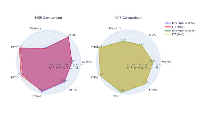
Figure 2: Average MSE and MAE comparison of our model and SOTA baselines with L = 720. The circle center represents the maximum possible error. Closer to the boundary indicates better performance.

5 Prediction Length Analysis and Ablation Study

5.1 Experimental Setup with Enhanced Architectures

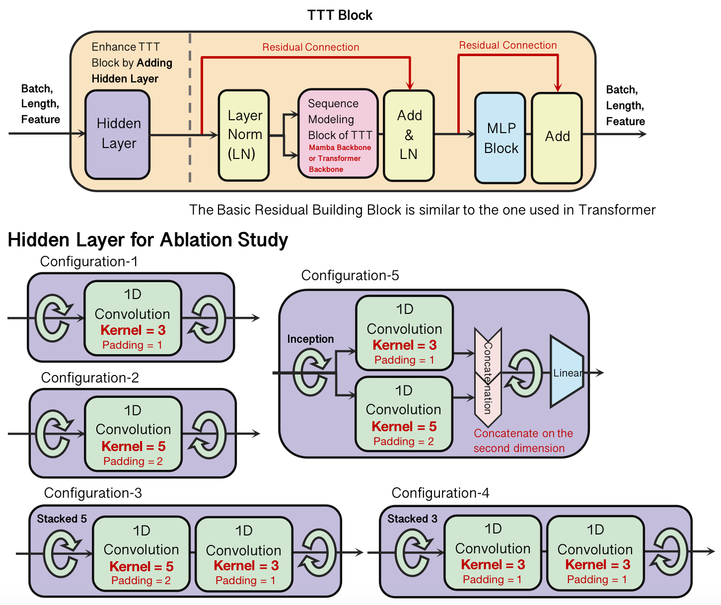
Figure 3: Convolutional Hidden Layer Added to the Beginning of the TTT Block. This basic residual building block is similar to the one used in Transformer models. We use the Hidden Layer as part of an ablation study to evaluate the effects of different hidden layer architectures on model performance. The five configurations are detailed below: (1) 1D Convolution with kernel size 3. (2) 1D Convolution with kernel size 5. (3) Two 1D Convolutions with kernel sizes 5 and 3 in cascade.(4) Two 1D Convolutions with kernel size 3 in cascade. (5) An Inception Block combining 1D Convolutions with kernel sizes 5 and 3, followed by concatenation and reduction to the original size. The Sequence Modeling Block of TTT can be used with two different backbones: the Mamba Backbone and the Transformer Backbone.

To assess the impact of enhancing the model architecture, we conducted experiments by adding hidden layer architectures before the sequence modeling block in each of the four TTT blocks. The goal was to improve performance by enriching feature extraction through local temporal context. As shown in Figure 3 in Appendix B.

We tested the following configurations: (1) Conv 3: 1D Convolution with kernel size 3, (2) Conv 5: 1D Convolution with kernel size 5, (3) Conv Stack 3: two 1D Convolutions with kernel size 3 in cascade, (4) Conv Stack 5: two 1D Convolutions with kernel sizes 5 and 3 in cascade, (5) Inception: an Inception Block combining 1D Convolutions with kernel sizes 5 and 3, followed by concatenation and reduction to the original size and (6) ModernTCN: A modern convolutional block proposed in [5] that uses depthwise and pointwise convolutions with residual connections similar to the structure of the transformer block. For the simpler architectures kernel sizes were limited to 5 to avoid oversmoothing, and original data dimensions were preserved to ensure consistency with the TTT architecture. For ModernTCN we reduced the internal dimensions to 16 (down from the suggested 64) and did not use multiscale due to the exponential increase in GPU memory required which slowed down the training process and did not allow the model to fit in a single A100 GPU. We kept the rest of the parameters of ModernTCN the same as in the original paper.

Ablation Study Findings

Our findings reveal that the introduction of additional hidden layer architectures, including convolutional layers, had varying degrees of impact on performance across different horizons. The best-performing setup was the Conv Stack 5 architecture, which achieved the lowest MSE and MAE at the 96 time horizon, with values of 0.261 and 0.289, respectively, outperforming the TimeMachine model at this horizon. At longer horizons, such as 336 and 720, Conv Stack 5 continued to show competitive performance, with a narrow gap between it and the TimeMachine model. For example, at the 720 horizon, Conv Stack 5 showed an MAE of 0.373, while TimeMachine had an MAE of 0.378.

However, other architectures, such as Conv 3 and Conv 5, provided only marginal improvements over the baseline TTT architectures (Linear and MLP). While they performed better than Linear and MLP, they did not consistently outperform more complex setups like Conv Stack 3 and 5 across all horizons. This suggests that hidden layer expressiveness can enhance model performance.

ModernTCN showed competitive results across multiple datasets (see Appendix D), such as ETTh2, where it achieved an MSE of 0.285 at horizon 96, outperforming Conv 3 and Conv 5. However, as with other deep convolutional layers, ModernTCN’s increased complexity also led to slower training times compared to simpler setups like Conv 3 and it failed to match Conv Stack 5’s performance.

5.2 Experimental Setup with Increased Prediction & Sequence Lengths

For the second part of our experiments, we extended the sequence and prediction lengths beyond the parameters tested in previous studies. We used the same baseline architectures (MLP and Linear) with the Mamba backbone as in the original TimeMachine paper, but this time also included the best-performing 1D Convolution architecture with kernel size 3.

The purpose of these experiments was to test the model’s capacity to handle much longer sequence lengths while maintaining high prediction accuracy. We tested the following sequence and prediction lengths, with $L=2880$ and $5760$, far exceeding the original length of $L=96$:

Seq Length	2880	2880	2880	2880	5760	5760	5760	5760	720	720	720	720
Pred Length	192	336	720	96	192	336	720	96	192	336	720	96

Table 2: Testing parameters for sequence and prediction lengths.

5.3 Results and Statistical Comparisons for Proposed Architectures

	Conv stack 5		TimeMachine		Conv 3		Conv 5		Conv stack 3		Inception		Linear		MLP
horizon	MSE	MAE	MSE	MAE	MSE	MAE	MSE	MAE	MSE	MAE	MSE	MAE	MSE	MAE	MSE	MAE
96	0.261	0.289	0.262	0.292	0.269	0.297	0.269	0.297	0.272	0.300	0.274	0.302	0.268	0.298	0.271	0.301
192	0.316	0.327	0.307	0.321	0.318	0.329	0.320	0.331	0.319	0.330	0.321	0.330	0.326	0.336	0.316	0.332
336	0.344	0.343	0.328	0.339	0.348	0.348	0.347	0.347	0.359	0.358	0.361	0.359	0.357	0.358	0.358	0.357
720	0.388	0.373	0.386	0.378	0.406	0.389	0.400	0.389	0.399	0.387	0.404	0.390	0.414	0.393	0.394	0.393

Table 3: MSE and MAE performance metrics for TimeMachine, TTT blocks with original architectures (MLP & Linear), and TTT block with different convolutional architectures across all prediction horizons.

The proposed architectures—TTT Linear, TTT MLP, Conv Stack 3, Conv Stack 5, Conv 3, Conv 5, Inception, and TTT with ModernTCN—exhibit varying performance across prediction horizons. TTT Linear performs well at shorter horizons (MSE 0.268, MAE 0.298 at horizon 96) but declines at longer horizons (MSE 0.357 at horizon 336). TTT MLP follows a similar trend with slightly worse performance. Conv 3 and Conv 5 outperform Linear and MLP at shorter horizons (MSE 0.269, MAE 0.297 at horizon 96) but lag behind Conv Stack models at longer horizons. TTT with ModernTCN shows promising results at shorter horizons, such as MSE 0.389, MAE 0.402 on ETTh1, and MSE 0.285, MAE 0.340 on ETTh2 at horizon 96. Although results for Traffic and Electricity datasets are pending, preliminary findings indicate TTT with ModernTCN is competitive, particularly for short-term dependencies (see Table 7 in Appendix D). Conv Stack 5 performs best at shorter horizons (MSE 0.261, MAE 0.289 at horizon 96). Inception provides stable performance across horizons, closely following Conv Stack 3 (MSE 0.361 at horizon 336). At horizon 720, Conv 5 shows a marginal improvement over Conv 3, with an MSE of 0.400 compared to 0.406. The Conv Stack 5 architecture demonstrates the best overall performance among all convolutional models.

5.4 Results and Statistical Comparisons for Increased Prediction and Sequence Lengths

	TTT		TimeMachine
Pred. Length	MSE	MAE	MSE	MAE
96	0.283	0.322	0.309	0.337
192	0.332	0.356	0.342	0.359
336	0.402	0.390	0.414	0.394
720	0.517	0.445	0.535	0.456
1440	0.399	0.411	0.419	0.429
2880	0.456	0.455	0.485	0.474
4320	0.580	0.534	0.564	0.523

Table 4: Average MSE and MAE for different prediction lengths and sequence length of 2880 comparing TimeMachine and TTT architectures.

	TTT		TimeMachine
Seq. Length	MSE	MAE	MSE	MAE
720	0.312	0.336	0.319	0.341
2880	0.366	0.384	0.373	0.388
5760	0.509	0.442	0.546	0.459

Table 5: Average MSE and MAE for different sequence lengths comparing TimeMachine and Conv stack 5 architectures.

Both shorter and longer sequence lengths affect model performance differently. Shorter sequence lengths (e.g., 2880) provide better accuracy for shorter prediction horizons, with the TTT model achieving an MSE of 0.332 and MAE of 0.356 at horizon 192, outperforming TimeMachine. Longer sequence lengths (e.g., 5760) result in higher errors, particularly for shorter horizons, but TTT remains more resilient, showing improved performance over TimeMachine. For shorter prediction lengths (96 and 192), TTT consistently yields lower MSE and MAE compared to TimeMachine. As prediction lengths grow to 720, both models experience increasing error rates, but TTT maintains a consistent advantage. For instance, at horizon 720, TTT records an MSE of 0.517 compared to TimeMachine’s 0.535. Overall, TTT consistently outperforms TimeMachine across most prediction horizons, particularly for shorter sequences and smaller prediction windows. As the sequence length increases, TTT’s ability to manage long-term dependencies becomes increasingly evident, with models like Conv Stack 5 showing stronger performance at longer horizons.

5.5 Evaluation

The results of our experiments indicate that the TimeMachine-TTT model outperforms the SOTA models across various scenarios, especially when handling larger sequence and prediction lengths. Several key trends emerged from the analysis:

• Improved Performance on Larger Datasets: On larger datasets, such as Electricity, Traffic, and Weather, TTT models demonstrated superior performance compared to TimeMachine. For example, at a prediction length of 96, the TTT architecture achieved an MSE of 0.283 compared to TimeMachine’s 0.309, reflecting a notable improvement. This emphasizes TTT’s ability to effectively handle larger temporal windows.

• Better Handling of Long-Range Dependencies: TTT-based models, particularly Conv Stack 5 and Conv 3, demonstrated clear advantages in capturing long-range dependencies. As prediction lengths increased, such as at 720, TTT maintained better error rates, with Conv Stack 5 achieving an MAE of 0.373 compared to TimeMachine’s 0.378. Although the difference narrows at longer horizons, the TTT architectures remain more robust, particularly in handling extended sequences and predictions.

• Impact of Hidden Layer Architectures: While stacked convolutional architectures, such as Conv Stack 3 and Conv Stack 5, provided incremental improvements, simpler architectures like Conv 3 and Conv 5 also delivered competitive performance. Conv Stack 5 showed a reduction in MSE compared to TimeMachine, at horizon 96, where it achieved an MSE of 0.261 versus TimeMachine’s 0.262. The ModernTCN architecture showed promising results, especially in capturing short-term dependencies effectively.

• Effect of Sequence and Prediction Lengths: As the sequence and prediction lengths increased, all models exhibited higher error rates. However, TTT-based architectures, particularly Conv Stack 5 and Conv 3, handled these increases better than TimeMachine. For example, at a sequence length of 5760 and prediction length of 720, TTT recorded lower MSE and MAE values, demonstrating better scalability and adaptability to larger contexts. Moreover, shorter sequence lengths (e.g., 2880) performed better at shorter horizons, while longer sequence lengths showed diminishing returns for short-term predictions.

6 Conclusion and Future Work

In this work, we improved the state-of-the-art (SOTA) model for time series forecasting by replacing the Mamba modules in the original TimeMachine model with Test-Time Training (TTT) modules, which leverage linear RNNs to capture long-range dependencies. Extensive experiments demonstrated that the TTT architectures—MLP and Linear—performed well, with MLP slightly outperforming Linear. Exploring alternative architectures, particularly Conv Stack 5 and ModernTCN, significantly improved performance at longer prediction horizons, with ModernTCN showing notable efficiency in capturing short-term dependencies. The most significant gains came from increasing sequence and prediction lengths, where our TTT models consistently matched or outperformed the SOTA model, particularly on larger datasets like Electricity, Traffic, and Weather, emphasizing the model’s strength in handling long-range dependencies. While convolutional stacks and ModernTCN showed promise, further improvements could be achieved by refining hidden layer configurations and exploring architectural diversity. Overall, this work demonstrates the potential of TTT modules in long-term forecasting, especially when combined with robust convolutional architectures and applied to larger datasets and longer horizons.

Appendix A Appendix A: TTT vs Mamba

Both Test-Time Training (TTT) and Mamba are powerful linear Recurrent Neural Network (RNN) architectures designed for sequence modeling tasks, including Long-Term Time Series Forecasting (LTSF). While both approaches aim to capture long-range dependencies with linear complexity, there are key differences in how they handle context windows, hidden state dynamics, and adaptability. This subsection compares the two, focusing on their theoretical formulations and practical suitability for LTSF.

A.1 Mamba: Gated Linear RNN via State Space Models (SSMs)

Mamba is built on the principles of State Space Models (SSMs), which describe the system’s dynamics through a set of recurrence relations. The fundamental state-space equation for Mamba is defined as:

$$h_{k}=\bar{A}h_{k-1}+\bar{B}u_{k},\quad v_{k}=Ch_{k},$$

where:

• $h_{k}$ represents the hidden state at time step $k$.

• $u_{k}$ is the input at time step $k$.

• $\bar{A}$ and $\bar{B}$ are learned state transition matrices.

• $v_{k}$ is the output at time step $k$, and $C$ is the output matrix.

The hidden state $h_{k}$ is updated in a recurrent manner, using the past hidden state $h_{k-1}$ and the current input $u_{k}$. Although Mamba can capture long-range dependencies better than traditional RNNs, its hidden state update relies on fixed state transitions governed by $\bar{A}$ and $\bar{B}$, which limits its ability to dynamically adapt to varying input patterns over time.

In the context of LTSF, while Mamba performs better than Transformer architectures in terms of computational efficiency (due to its linear complexity in relation to sequence length), it still struggles to fully capture long-term dependencies as effectively as desired. This is because the fixed state transitions constrain its ability to adapt dynamically to changes in the input data.

A.2 TTT: Test-Time Training with Dynamic Hidden States

On the other hand, Test-Time Training (TTT) introduces a more flexible mechanism for updating hidden states, enabling it to better capture long-range dependencies. TTT uses a trainable hidden state that is continuously updated at test time, allowing the model to adapt dynamically to the current input. The hidden state update rule for TTT can be defined as:

$$z_{t}=f(x_{t};W_{t}),\quad W_{t}=W_{t-1}-\eta\nabla\ell(W_{t-1};x_{t}),$$

where:

• $z_{t}$ is the hidden state at time step $t$, updated based on the input $x_{t}$.

• $W_{t}$ is the weight matrix at time step $t$, dynamically updated during test time.

• $\ell(W;x_{t})$ is the loss function, typically computed as the difference between the predicted and actual values: $\ell(W;x_{t})=\|f(\tilde{x}_{t};W)-x_{t}\|^{2}$.

• $\eta$ is the learning rate for updating $W_{t}$ during test time.

The key advantage of TTT over Mamba is the dynamic nature of its hidden states. Rather than relying on fixed state transitions, TTT continuously adapts its parameters based on new input data at test time. This enables TTT to have an infinite context window, as it can effectively adjust its internal representation based on all past data and current input. This dynamic adaptability makes TTT particularly suitable for LTSF tasks, where capturing long-term dependencies is crucial for accurate forecasting.

A.3 Comparison of Complexity and Adaptability

One of the major benefits of both Mamba and TTT is their linear complexity with respect to sequence length. Both models avoid the quadratic complexity of Transformer-based architectures, making them efficient for long time series data. However, TTT offers a distinct advantage in terms of adaptability:

• Mamba:

  $$\mathcal{O}(L\times D^{2}),$$

  where $L$ is the sequence length and $D$ is the dimension of the state space. Mamba’s fixed state transition matrices limit its expressiveness over very long sequences.

• TTT:

  $$\mathcal{O}(L\times N\times P),$$

  where $N$ is the number of dynamic parameters (weights) and $P$ is the number of iterations for test-time updates. The dynamic nature of TTT allows it to capture long-term dependencies more effectively, as it continuously updates the weights $W_{t}$ during test time.

Theoretically, TTT is more suitable for LTSF due to its ability to model long-range dependencies dynamically. By continuously updating the hidden states based on both past and present data, TTT effectively functions with an infinite context window, whereas Mamba is constrained by its fixed state-space formulation. Moreover, TTT is shown to be theoretically equivalent to self-attention under certain conditions, meaning it can model interactions between distant time steps in a similar way to Transformers but with the added benefit of linear complexity. This makes TTT not only computationally efficient but also highly adaptable to the long-term dependencies present in time series data.

In summary, while Mamba provides significant improvements over traditional RNNs and Transformer-based models, its reliance on fixed state transitions limits its effectiveness in modeling long-term dependencies. TTT, with its dynamic hidden state updates and theoretically infinite context window, is better suited for Long-Term Time Series Forecasting (LTSF) tasks. TTT’s ability to adapt its parameters at test time ensures that it can handle varying temporal patterns more flexibly, making it the superior choice for capturing long-range dependencies in time series data.

Appendix B Appendix B: Model Components

B.1 TTT Block and Proposed Architectures

Below we illustrate the components of the TTT block and the proposed architectures we used in our ablation study for the model based on convolutional blocks:

B.2 Prediction

The prediction process in our model works as follows. During inference, the input time series $(\mathbf{x}_{1},\dots,\mathbf{x}_{L})$, where $L$ is the look-back window length, is split into $M$ univariate series $\mathbf{x}^{(i)}\in\mathbb{R}^{1\times L}$. Each univariate series represents one channel of the multivariate time series. Specifically, an individual univariate series can be denoted as:

$$\mathbf{x}^{(i)}_{1:L}=\left(x^{(i)}_{1},\dots,x^{(i)}_{L}\right)\quad\text{where }i=1,\dots,M.$$

Each of these univariate series is fed into the model, and the output of the model is a predicted series $\hat{\mathbf{x}}^{(i)}$ for each input channel. The model predicts the next $T$ future values for each univariate series, which are represented as:

$$\hat{\mathbf{x}}^{(i)}=\left(\hat{x}^{(i)}_{L+1},\dots,\hat{x}^{(i)}_{L+T}\right)\in\mathbb{R}^{1\times T}.$$

Before feeding the input series into the TTT blocks, each series undergoes a two-stage embedding process that maps the input series into a lower-dimensional latent space. This embedding process is crucial for allowing the model to learn meaningful representations of the input data. The embedding process is mathematically represented as follows:

$$\mathbf{x}^{(1)}=E_{1}(\mathbf{x}^{(0)}),\quad\mathbf{x}^{(2)}=E_{2}(DO(\mathbf{x}^{(1)})),$$

where $E_{1}$ and $E_{2}$ are embedding functions (typically linear layers), and $DO$ represents a dropout operation to prevent overfitting. The embeddings help the model process the input time series more effectively and ensure robustness during training and inference.

B.3 Normalization

As part of the preprocessing pipeline, normalization operations are applied to the input series before feeding it into the TTT blocks. The input time series $\mathbf{x}$ is normalized into $\mathbf{x}^{0}$, represented as:

$$\mathbf{x}^{0}=\left[\mathbf{x}^{(0)}_{1},\dots,\mathbf{x}^{(0)}_{L}\right]\in\mathbb{R}^{M\times L}.$$

We experiment with two different normalization techniques:

• Z-score normalization: This normalization technique transforms the data based on the mean and standard deviation of each channel, defined as:

  $$x^{(0)}_{i,j}=\frac{x_{i,j}-\text{mean}(x_{i,:})}{\sigma_{j}},$$

  where $\sigma_{j}$ is the standard deviation of channel $j$, and $j=1,\dots,M$.

• Reversible Instance Normalization (RevIN) [13]: RevIN normalizes each channel based on its mean and variance but allows the normalization to be reversed after the model prediction, which ensures the output predictions are on the same scale as the original input data. We choose to use RevIN in our model because of its superior performance, as demonstrated in [1].

Once the model has generated the predictions, RevIN Denormalization is applied to map the normalized predictions back to the original scale of the input data, ensuring that the model outputs are interpretable and match the scale of the time series used during training.

Appendix C Appendix C: Analysis on Increased Prediction and Sequence Length

C.1 Effect of Sequence Length

Shorter Sequence Lengths (e.g., 2880)

Shorter sequence lengths tend to offer better performance for shorter prediction horizons. For instance, with a sequence length of 2880 and a prediction length of 192, the TTT model achieves an MSE of 0.332 and an MAE of 0.356, outperforming TimeMachine, which has an MSE of 0.342 and an MAE of 0.359. This indicates that shorter sequence lengths allow the model to focus on immediate temporal patterns, improving short-horizon accuracy.

Longer Sequence Lengths (e.g., 5760)

Longer sequence lengths show mixed performance, particularly at shorter prediction horizons. For example, with a sequence length of 5760 and a prediction length of 192, the TTT model’s MSE rises to 0.509 and MAE to 0.442, which is better than TimeMachine’s MSE of 0.546 and MAE of 0.459. While the performance drop for TTT is less severe than for TimeMachine, longer sequence lengths can introduce unnecessary complexity, leading to diminishing returns for short-term predictions.

C.2 Effect of Prediction Length

Shorter Prediction Lengths (96, 192)

Shorter prediction lengths consistently result in lower error rates across all models. For instance, at a prediction length of 96 with a sequence length of 2880, the TTT model achieves an MSE of 0.283 and an MAE of 0.322, outperforming TimeMachine’s MSE of 0.309 and MAE of 0.337. This demonstrates that both models perform better with shorter prediction lengths, as fewer dependencies need to be captured.

Longer Prediction Lengths (720)

As prediction length increases, both MSE and MAE grow for both models. At a prediction length of 720 with a sequence length of 2880, the TTT model records an MSE of 0.517 and an MAE of 0.445, outperforming TimeMachine, which has an MSE of 0.535 and MAE of 0.456. This shows that while error rates increase with longer prediction horizons, TTT remains more resilient in handling longer-term dependencies than TimeMachine.

Appendix D Appendix D: Tables

Dataset	Channels	Time Points	Frequencies
Weather	21	52696	10 Minutes
Traffic	862	17544	Hourly
Electricity	321	26304	Hourly
ETTh1	7	17420	Hourly
ETTh2	7	17420	Hourly
ETTm1	7	69680	15 Minutes
ETTm2	7	69680	15 Minutes

Table 6: Details of each dataset

TTT with ModernTCN
	ETTh1		ETTh2		ETTm1		ETTm2		Weather		Traffic		Electricity
	MSE	MAE	MSE	MAE	MSE	MAE	MSE	MAE	MSE	MAE	MSE	MAE	MSE	MAE
96	0.389	0.402	0.285	0.340	0.322	0.362	0.189	0.273	0.165	0.209	*	*	*	*
192	0.425	0.422	0.359	0.386	0.385	0.397	0.251	0.310	0.265	0.281	*	*	*	*
366	0.460	0.442	0.351	0.388	0.415	0.416	0.309	0.344	0.269	0.293	*	*	*	*
720	0.485	0.475	0.439	0.449	0.490	0.454	0.410	0.403	*	*	*	*	*	*

Table 7: TTT with ModernTCN results on different datasets. Star symbol indicates that experiment is still running.

References

- [1] Md Atik Ahamed and Qiang Cheng. Timemachine: A time series is worth 4 mambas for long-term forecasting, 2024. URL: https://arxiv.org/abs/2403.09898, arXiv:2403.09898.
- [2] Si-An Chen, Chun-Liang Li, Nate Yoder, Sercan O. Arik, and Tomas Pfister. Tsmixer: An all-mlp architecture for time series forecasting, 2023. URL: https://arxiv.org/abs/2303.06053, arXiv:2303.06053.
- [3] Xupeng Chen, Ran Wang, Amirhossein Khalilian-Gourtani, Leyao Yu, Patricia Dugan, Daniel Friedman, Werner Doyle, Orrin Devinsky, Yao Wang, and Adeen Flinker. A neural speech decoding framework leveraging deep learning and speech synthesis. Nature Machine Intelligence, pages 1–14, 2024.
- [4] Abhimanyu Das, Weihao Kong, Andrew Leach, Shaan Mathur, Rajat Sen, and Rose Yu. Long-term forecasting with tide: Time-series dense encoder, 2024. URL: https://arxiv.org/abs/2304.08424, arXiv:2304.08424.
- [5] Luo Donghao and Wang Xue. ModernTCN: A modern pure convolution structure for general time series analysis. In The Twelfth International Conference on Learning Representations, 2024. URL: https://openreview.net/forum?id=vpJMJerXHU.
- [6] Alexey Dosovitskiy, Lucas Beyer, Alexander Kolesnikov, Dirk Weissenborn, Xiaohua Zhai, Thomas Unterthiner, Mostafa Dehghani, Matthias Minderer, Georg Heigold, Sylvain Gelly, Jakob Uszkoreit, and Neil Houlsby. An image is worth 16x16 words: Transformers for image recognition at scale. In 9th International Conference on Learning Representations, ICLR 2021, Virtual Event, Austria, May 3-7, 2021. OpenReview.net, 2021. URL: https://openreview.net/forum?id=YicbFdNTTy.
- [7] Albert Gu and Tri Dao. Mamba: Linear-time sequence modeling with selective state spaces, 2024. URL: https://arxiv.org/abs/2312.00752, arXiv:2312.00752.
- [8] Albert Gu, Karan Goel, and Christopher Ré. Efficiently modeling long sequences with structured state spaces, 2022. URL: https://arxiv.org/abs/2111.00396, arXiv:2111.00396.
- [9] Albert Gu, Ankit Gupta, Karan Goel, and Christopher Ré. On the parameterization and initialization of diagonal state space models, 2022. URL: https://arxiv.org/abs/2206.11893, arXiv:2206.11893.
- [10] Ankit Gupta, Harsh Mehta, and Jonathan Berant. Simplifying and understanding state space models with diagonal linear rnns, 2023. URL: https://arxiv.org/abs/2212.00768, arXiv:2212.00768.
- [11] Haowen Hou and F. Richard Yu. Rwkv-ts: Beyond traditional recurrent neural network for time series tasks, 2024. URL: https://arxiv.org/abs/2401.09093, arXiv:2401.09093.
- [12] Taesung Kim, Jinhee Kim, Yunwon Tae, Cheonbok Park, Jang-Ho Choi, and Jaegul Choo. Reversible instance normalization for accurate time-series forecasting against distribution shift. In International Conference on Learning Representations, 2021.
- [13] Taesung Kim, Jinhee Kim, Yunwon Tae, Cheonbok Park, Jang-Ho Choi, and Jaegul Choo. Reversible instance normalization for accurate time-series forecasting against distribution shift. In International Conference on Learning Representations, 2022. URL: https://openreview.net/forum?id=cGDAkQo1C0p.
- [14] Zhe Li, Shiyi Qi, Yiduo Li, and Zenglin Xu. Revisiting long-term time series forecasting: An investigation on linear mapping, 2023. URL: https://arxiv.org/abs/2305.10721, arXiv:2305.10721.
- [15] Minhao Liu, Ailing Zeng, Muxi Chen, Zhijian Xu, Qiuxia Lai, Lingna Ma, and Qiang Xu. Scinet: Time series modeling and forecasting with sample convolution and interaction, 2022. URL: https://arxiv.org/abs/2106.09305, arXiv:2106.09305.
- [16] Shizhan Liu, Hang Yu, Cong Liao, Jianguo Li, Weiyao Lin, Alex X Liu, and Schahram Dustdar. Pyraformer: Low-complexity pyramidal attention for long-range time series modeling and forecasting. In International Conference on Learning Representations, 2022.
- [17] Yong Liu, Tengge Hu, Haoran Zhang, Haixu Wu, Shiyu Wang, Lintao Ma, and Mingsheng Long. itransformer: Inverted transformers are effective for time series forecasting. arXiv preprint arXiv:2310.06625, 2023.
- [18] Yong Liu, Tengge Hu, Haoran Zhang, Haixu Wu, Shiyu Wang, Lintao Ma, and Mingsheng Long. itransformer: Inverted transformers are effective for time series forecasting, 2024. URL: https://arxiv.org/abs/2310.06625, arXiv:2310.06625.
- [19] Yong Liu, Haixu Wu, Jianmin Wang, and Mingsheng Long. Non-stationary transformers: Exploring the stationarity in time series forecasting, 2023. URL: https://arxiv.org/abs/2205.14415, arXiv:2205.14415.
- [20] Haowei Ni, Shuchen Meng, Xieming Geng, Panfeng Li, Zhuoying Li, Xupeng Chen, Xiaotong Wang, and Shiyao Zhang. Time series modeling for heart rate prediction: From arima to transformers. arXiv preprint arXiv:2406.12199, 2024.
- [21] Yuqi Nie, Nam H. Nguyen, Phanwadee Sinthong, and Jayant Kalagnanam. A time series is worth 64 words: Long-term forecasting with transformers, 2023. URL: https://arxiv.org/abs/2211.14730, arXiv:2211.14730.
- [22] Antonio Orvieto, Samuel L Smith, Albert Gu, Anushan Fernando, Caglar Gulcehre, Razvan Pascanu, and Soham De. Resurrecting recurrent neural networks for long sequences. In Proceedings of the 40th International Conference on Machine Learning, ICML’23. JMLR.org, 2023.
- [23] Badri N. Patro and Vijay S. Agneeswaran. Simba: Simplified mamba-based architecture for vision and multivariate time series, 2024. URL: https://arxiv.org/abs/2403.15360, arXiv:2403.15360.
- [24] Yu Sun, Xinhao Li, Karan Dalal, Jiarui Xu, Arjun Vikram, Genghan Zhang, Yann Dubois, Xinlei Chen, Xiaolong Wang, Sanmi Koyejo, Tatsunori Hashimoto, and Carlos Guestrin. Learning to (learn at test time): Rnns with expressive hidden states, 2024. URL: https://arxiv.org/abs/2407.04620, arXiv:2407.04620.
- [25] Ashish Vaswani, Noam Shazeer, Niki Parmar, Jakob Uszkoreit, Llion Jones, Aidan N Gomez, Ł ukasz Kaiser, and Illia Polosukhin. Attention is all you need. In I. Guyon, U. Von Luxburg, S. Bengio, H. Wallach, R. Fergus, S. Vishwanathan, and R. Garnett, editors, Advances in Neural Information Processing Systems, volume 30. Curran Associates, Inc., 2017. URL: https://proceedings.neurips.cc/paper_files/paper/2017/file/3f5ee243547dee91fbd053c1c4a845aa-Paper.pdf.
- [26] Qingsong Wen, Tian Zhou, Chaoli Zhang, Weiqi Chen, Ziqing Ma, Junchi Yan, and Liang Sun. Transformers in time series: A survey, 2023. URL: https://arxiv.org/abs/2202.07125, arXiv:2202.07125.
- [27] Haixu Wu, Tengge Hu, Yong Liu, Hang Zhou, Jianmin Wang, and Mingsheng Long. Timesnet: Temporal 2d-variation modeling for general time series analysis, 2023. URL: https://arxiv.org/abs/2210.02186, arXiv:2210.02186.
- [28] Haixu Wu, Jiehui Xu, Jianmin Wang, and Mingsheng Long. Autoformer: Decomposition transformers with auto-correlation for long-term series forecasting, 2022. URL: https://arxiv.org/abs/2106.13008, arXiv:2106.13008.
- [29] Ailing Zeng, Muxi Chen, Lei Zhang, and Qiang Xu. Are transformers effective for time series forecasting?, 2022. URL: https://arxiv.org/abs/2205.13504, arXiv:2205.13504.
- [30] Yunhao Zhang and Junchi Yan. Crossformer: Transformer utilizing cross-dimension dependency for multivariate time series forecasting. In International Conference on Learning Representations, 2023. URL: https://openreview.net/forum?id=vSVLM2j9eie.
- [31] Haoyi Zhou, Shanghang Zhang, Jieqi Peng, Shuai Zhang, Jianxin Li, Hui Xiong, and Wancai Zhang. Informer: Beyond efficient transformer for long sequence time-series forecasting, 2021. URL: https://arxiv.org/abs/2012.07436, arXiv:2012.07436.
- [32] Tian Zhou, Ziqing Ma, Qingsong Wen, Xue Wang, Liang Sun, and Rong Jin. Fedformer: Frequency enhanced decomposed transformer for long-term series forecasting, 2022. URL: https://arxiv.org/abs/2201.12740, arXiv:2201.12740.