Superconvergence of the local discontinuous Galerkin method with generalized numerical fluxes for one-dimensional linear time-dependent fourth-order equations
Abstract
In this paper, we concentrate on the superconvergence of the local discontinuous Galerkin method with generalized numerical fluxes for one-dimensional linear time-dependent fourth-order equations. The adjustable numerical viscosity of the generalized numerical fluxes is beneficial for long time simulations with a slower error growth. By using generalized Gauss–Radau projections and correction functions together with a suitable numerical initial condition, we derive, for polynomials of degree , th order superconvergence for the numerical flux and cell averages, th order superconvergence at generalized Radau points, and th order for error derivative at generalized Radau points. Moreover, a supercloseness result of order is established between the generalized Gauss–Radau projection and the numerical solution. Superconvergence analysis of mixed boundary conditions is also given. Equations with discontinuous initial condition and nonlinear convection term are numerically investigated, illustrating that the conclusions are valid for more general cases.
Keywords
Local discontinuous Galerkin method, Linear fourth-order equation, Superconvergence, Correction function, generalized Gauss–Radau projection.
AMS subject classifications
65M12, 65M15, 65M60
1 Introduction
In this paper, we investigate superconvergence of local discontinuous Galerkin (LDG) methods with generalized numerical fluxes for one-dimensional linear fourth-order problem
| (1.1a) | |||||
| (1.1b) | |||||
where and are constant, and . Periodic and mixed boundary conditions are considered. Note that, in (1.1a), dominates in spite of the anti-diffusion term with . The generalized numerical fluxes with flexible numerical viscosities allow us to obtain a slower error growth for long time simulations, when compared with the LDG scheme using the upwind and alternating fluxes; see Figure 6.1 below. With the help of correction functions and an elaborate numerical initial condition, by establishing a superconvergent bound for interpolation errors, supercongence for the numerical flux, cell averages, Radau points as well as supercloseness are derived.
The discontinuous Galerkin (DG) method, allowing discontinuities across cell boundaries in the finite element space, was proposed mainly for solving hyperbolic conservation laws and systems [8, 7, 10]. In [9], the LDG method was developed for solving convection-diffusion equations, which was achieved by introducing an auxiliary variable and rewriting the original problem into a first-order system to which the DG method can be applied. Later, the LDG methods have been widely adopted to solve high-order partial differential equations (PDEs), such as Korteweg–de Vries (KdV) type equations [25], Schrödinger equations [23], the Zakharov–Kuznetsov equation [24], and viscous Burgers equations [12]. For more details of DG and LDG methods, we refer to the review paper [21].
The fourth-order PDEs have numerous physical and engineering applications. For example, fourth-order boundary value problems can describe the bending of an elastic beam, and the Cahn–Hilliard equation reflects the process of phase separation, in which the properties of fluid thermodynamics transfer smoothly from one phase to another [2]. DG and LDG methods have been studied for solving fourth-order PDEs. In [11], Dong and Shu used the LDG method for fourth-order time-dependent problems to obtain optimal error estimates in one- and multi-dimensional spaces. A free-energy stable DG method for the Cahn–Hilliard equation with non-conforming elements was developed in [20].
Superconvergence of DG and LDG methods has gained more attention in recent years. Based on the correction function technique, in [5], Cao et al. proved superconvergence of numerical fluxes, cell averages and Radau points of DG methods for linear hyperbolic equations. Superconvergence of LDG methods for high-order linear problems was given in [3]. Superconvergence of ultraweak-LDG method for linear fourth-order equations can be found in [16]. We would like to emphasize that superconvergence property is probably sensitive to the numerical initial condition and a special initial discretization should be chosen. In addition, based on Fourier analysis, [19] studied the superconvergence properties of various direct DG methods for diffusion equations, and presented quantitative errors at Lobatto points.
In the design of DG and LDG schemes, the choice of numerical fluxes plays an important role to guarantee stability and optimal order of accuracy. For linear hyperbolic equations, instead of using classical monotone or upwind fluxes, [18] proposed a nonmonotone upwind-biased flux and showed -stability as well as optimal error estimates, in which a global generalized Gauss–Radau (GGR) projection is constructed. Almost at the same time, the GGR projection is considered in LDG methods for solving the Burgers–Poisson equation in [14]. The generalized alternating fluxes were then developed for LDG methods solving linear convection-diffusion equations [6], in which a modified GGR projection is designed to deal with different weighs of generalized numerical fluxes. For the Vlasov-viscous Burgers system, a coupling DG and LDG method with generalized numerical fluxes was introduced in [12], which is mass and momentum conservative. Moreover, superconvergence of DG methods with upwind-biased fluxes for linear hyperbolic equations and LDG methods with generalized alternating fluxes for linear convection-diffusion equations were given in [4] and [15], respectively.
Generalized fluxes with flexible numerical viscosities may be useful for long time simulations, as shown in Figure 6.1. It would be interesting to investigate superconvergence of LDG methods for linear fourth-order problems, especially when generalized fluxes with different weights are concerned. The superconvergence analysis mainly involves two difficulties. One is that the correction function is globally coupled, which can be solved by the property of circulant matrices. The other difficulty is a proper choice of numerical initial condition, which is achieved by the exact collocation for the third order derivative. Superconvergent initial error estimates can be obtained by using the discrete Poincaré inequality and the relationship between the derivative a numerical solution and another auxiliary variable.
The paper is organized as follows. In Section 2, we present the LDG scheme using generalized numerical fluxes for one-dimensional fourth-order problem with periodic boundary conditions and introduce some preliminaries regarding GGR projections as well as properties of DG operators. In Section 3, we construct correction functions with superconvergence property and derive a superconvergent bound for interpolation errors. Section 4 is the main body of the paper, in which a suitable numerical initial condition is chosen, and a supercloseness result between the interpolation function and the LDG solution is established, followed by superconvergence of numerical fluxes, cell averages and Radau points. Extension to mixed boundary conditions is provided in Section 5. In Section 6, numerical experiments with linear equations as well as nonperiodic boundary conditions are given to validate theoretical results, and problems with discontinuous initial condition and nonlinear convection term are presented to illustrate that the superconvergent results hold for more general cases. We end in Section 7 with conclusions and perspectives for future work.
2 The LDG scheme and preliminaries
Without loss of generality, consider in (1.1), i.e.,
| (2.1a) | |||||
| (2.1b) | |||||
where . To clearly display superconvergence analysis of LDG methods with generalized numerical fluxes, we mainly consider periodic boundary conditions, and the case with mixed boundary conditions is discussed in Section 5.
2.1 The LDG scheme
We adopt the following standard notation. Consider a partition , where, for any positive integer , . The cell center and cell length are denoted by and , respectively. Denote , , and use to represent the set of cell boundary points. Assume that the mesh is quasi uniform, i.e., there is a positive constant such that , . The DG finite element space is
where is the space of polynomials of degree at most in .
For any integer , the Sobolev space in is denoted as equipped with the norm , and, when , and . Here and below, the index or will be omitted when or , and an unmarked norm is the standard norm in . For , we denote the broken Sobolev spaces as
with the norm
Moreover, the norm for boundaries is and the seminorm
| (2.2) |
with , where are limits from the right and left cells. means that can be bounded by multiplied by a positive constant independent of .
To define the LDG scheme, we rewrite (2.1a) into a first-order system
Then, the semi-discrete LDG scheme for solving (2.1) is to find , , , and such that
| (2.3a) | ||||
| (2.3b) | ||||
| (2.3c) | ||||
| (2.3d) | ||||
hold for all , , and and . Here and below, denotes the inner product in with , and
| (2.4) |
The following generalized numerical fluxes with two weights are chosen, namely
| (2.5) |
where, for , and .
2.2 Preliminaries
For , the GGR projection [6] is defined as the unique function in satisfying
| (2.6a) | ||||||
| (2.6b) | ||||||
which has the following optimal approximation property
| (2.7) |
where is independent of .
Consider the Legendre expansion
where denotes the rescaled Legendre polynomial of degree in . It follows from the orthogonality of in (2.6a) that
and can be determined by (2.6b). Consequently,
| (2.8) |
The Bramble–Hilbert lemma and scaling arguments yield
| (2.9) |
which will be used later in the superconvergence analysis of correction functions in Section 3.1.
In the construction of correction functions, the following integral operator is useful, as defined in [4]
| (2.10) |
Clearly, . If is taken as , we have, by the recurrence relationships of Legendre polynomials,
| (2.11) |
In the analysis of generalized fluxes with different weights, the following generalized skew-symmetry property is needed, as shown in [13]. It reads, for and weights ,
| (2.12) |
Also, the discrete Poincaré inequality in [1] is helpful in deriving superconvergent initial error estimates. That is, for , there holds
| (2.13) |
where , has been defined in (2.2) and is independent of . Moreover, the following inverse inequalities are necessary, namely for
| (2.14) |
where is independent of .
Let us finish this section by showing a lemma concerning the relationship between the norm of derivative, the jump seminorm of LDG solutions and the norm of the adjacent auxiliary variable, when the LDG scheme with generalized numerical fluxes is considered. Using the same approach as that in [22], we have the following lemma.
3 Correction functions and interpolation functions
To obtain superconvergence property, we construct correction functions in Section 3.1, and establish a superconvergent bound of interpolation errors in Section 3.2.
3.1 Correction functions
We start by constructing a series of functions , , and , satisfying
| (3.1a) | |||||
| (3.1b) | |||||
| (3.1c) | |||||
| (3.1d) | |||||
for and , where
| (3.2) |
Then, for , the correction functions are defined by
| (3.3) |
Superconvergence of is shown in the following lemma.
Lemma 3.1.
Proof.
We prove this lemma by induction. For , denote
where are coefficients to be determined later.
Step 1: For , choosing () in (3.1a) with , and taking into account (3.2) together with (2.11), we arrive at the following equality
where is the coefficient in (2.8) with , replaced by , , respectively. Using the same procedure for (3.1b)–(3.1d), we obtain, by the orthogonality of Legendre polynomials, the expression
| (3.6) |
where
| (3.7) |
In what follows, let us concentrate on , for and . Using the boundary collocations in (3.1) and the fact that , , we get
| (3.8) |
where and . Consequently, the linear system (3.8) can be written in the matrix-vector form
| (3.9) |
where
and
is an circulant matrix and The determinant of is
where . Thus, is always invertible for and the linear system (3.9) has unique solutions. Moreover, the inverse of ,
is also circulant. After a direct calculation, we have
where are entries of the -th row of . By (2.9), (3.7)–(3.8), we get
This, together with (3.6) and (2.9), produces
and thus (3.4) holds for .
Step 2: Assume that (3.4) is valid for and we want to show it still holds for . By induction hypothesis together with an argument similar to that in deriving (3.6), we have
Choosing , , in (3.1a) and recalling (2.11), we obtain
Using the same procedure for (3.1b)–(3.1d), we get, by the orthogonality of Legendre polynomials,
where
and
Thus, we obtain the following system
| (3.10) |
where , and , respectively. Again, the above linear system can be rewritten as a matrix-vector form as that in (3.9). When , we can establish the uniqueness, existence of (3.10) and obtain
| (3.11) |
It is easy to show, for with , that
Analogously,
Therefore, (3.4) is valid for with . This finishes the proof of Lemma 3.1. ∎
3.2 A superconvergent bound of interpolation errors
By the LDG scheme (2.3) and Galerkin orthogonality, we get error equations
| (3.12a) | ||||
| (3.12b) | ||||
| (3.12c) | ||||
| (3.12d) | ||||
where with . We use the following decomposition
| (3.13a) | ||||
| and introduce the interpolation function | ||||
| (3.13b) | ||||
with the GGR projection () given in (2.6) and the correction function defined in (3.3).
A superconvergent bound of interpolation errors is presented in the following lemma.
Lemma 3.2.
Proof.
In what follows, let us show (3.14d) only, and proofs for (3.14a)–(3.14c) are analogous. To do that, for and , since , we deduce from (2.4) and (3.1) that
Consequently, for the left hand side of (3.14d), one has
| (3.15a) | ||||
| For , we now employ integration by parts and the definition of correction functions in (3.1d) to conclude that | ||||
| (3.15b) | ||||
where we have also used the fact that
implied by the definition of integral operator in (2.10) and the orthogonality of in (3.4b).
4 Superconvergence
In this section, we first introduce a suitable numerical initial condition satisfying superconvergent property in Section 4.1, then show supercloseness between interpolation functions and LDG solutions in Section 4.2, and derive superconvergence concerning numerical flux, cell averages and generalized Radau points in Section 4.3.
By the error decomposition (3.13a) and using the same argument as that in deriving (3.16) in the proof of Lemma 3.2, we sum the error equations (3.12) over all to obtain
| (4.1a) | ||||
| (4.1b) | ||||
| (4.1c) | ||||
| (4.1d) | ||||
4.1 The numerical initial condition
To be compatible with superconvergent property, a suitable choice of numerical initial condition is constructed as follows. For and (), choose
| (4.2) |
with , and being the solutions to
| (4.3a) | ||||
| (4.3b) | ||||
| (4.3c) | ||||
where . Existence, uniqueness as well as superconvergent initial error estimates for the above numerical initial condition are established in the following lemma.
Lemma 4.1.
Proof.
Let us start by showing unique existence, and taking as an example. To do that, we need the following conservation property of ,
| (4.4) |
which is obtained by taking in (4.3b), summing over all and using the definition of DG operator in (2.4), i.e.,
in combination with periodic boundary conditions and Galerkin orthogonality. For , suppose and are the solutions of (4.3a) with satisfying (4.2). Denoting , it follows from (4.3a) and (4.4) that
which, by letting , summing over all and using the identity (2.12), implies
This indicates that is constant in . Since , we conclude that
Therefore, is unique, and thus for . Since (4.3) is a linear system, the existence follows immediately. When , the scheme (2.3a) is still valid due to the continuity of numerical solutions with respect to time. This allows us to derive the conservation property of , and thus unique existence follows.
We now move on to the estimate of , and the estimates to , are analogous. By using (4.1b) and in (4.2), we have
which, by Lemma 2.1, yields
| (4.5) |
Using the orthogonality of in (2.6a) and in (3.4b), we have
Summing the above equation over all and taking into account (4.4), we arrive at
| (4.6) |
We are now ready to estimate . It reads
where in the second step we have used (4.6) and the discrete Poincaré inequality with in (2.13), and in the last step we have employed (4.5). Consequently, by (3.4a) in Lemma 3.1, we get
where depends on , but is independent of .
To finish the proof of Lemma 4.1, it remains to show a bound for . Due to the continuity with respect to time, (4.1a) is still valid for . Since , we rewrite (4.1a) to get
where we have also used (4.1c)–(4.1d). Letting , by using Young’s inequality and (3.4a) in Lemma 3.1, we have, at ,
which is,
Then, by using the estimates of and , we have
where depends on and , but is independent of . This completes the proof of Lemma 4.1. ∎
4.2 Supercloseness
The supercloseness between interpolation functions and LDG solutions is given in the following theorem.
Theorem 4.1.
Suppose is the exact solution of the fourth-order problem (2.1) with periodic boundary conditions, which is sufficiently smooth, e.g., , . Assume that () are LDG solutions to (2.3) with generalized fluxes (2.5) and . Let and interpolation functions be defined in (3.13a)–(3.13b) . Then, under the numerical initial condition (4.2)–(4.3), we have the following supercloseness result
| (4.7) |
where depends on and , but is independent of .
Proof.
First, taking in (4.1a)–(4.1d) and adding them together, by using the generalized skew-symmetry property in (2.12), namely,
| (4.8) |
we get
| (4.9) |
Utilizing identity (2.12) with the same weight , we have
since . Taking in (4.1c), we obtain
Consequently, (4.9) becomes
By using Young’s inequality and (3.4a) in Lemma 3.1, we have
which is,
| (4.10) |
Next, we take the time derivative of (4.1d) and choose in (4.1a)–(4.1c) and the newly obtained (4.1d). Summing them together and using the generalized skew-symmetry property in (2.12) with , namely,
we obtain
| (4.11) |
Taking in (4.1d), we get
Taking in (4.1b), and using the generalized skew-symmetry property in (4.8), we derive
Consequently, (4.11) becomes
Utilizing Young’s inequality and (3.4a) in Lemma 3.1, we obtain
| (4.12) |
where
and depends on and , but is independent of .
Now, summing (4.10) and (4.12) together, we have
| (4.13) |
where satisfies, by integration by parts with respect to time,
It implies that, by using Young’s inequality, (3.4a) in Lemma 3.1 and the estimate of in Lemma 4.1,
| (4.14) |
where depends on and , but is independent of . Integrating (4.13) with respect to time from to , we get, by (4.14)
This, together with estimates of and in Lemma 4.1, produces
where depends on and , but is independent of . A straightforward application of Gronwall’s inequality gives us the desired result (4.7). This completes the proof of Theorem 4.1. ∎
4.3 Superconvergence
To show superconvergent results at generalized Radau points, we begin by recalling the generalized Radau polynomials [4]
defined in . Then, we rescale to to get , and denote the roots of and by and , respectively, where and . Accordingly, for any positive weight , a local projection can be defined as that in [4], namely
which satisfies the following lemma.
Lemma 4.2.
[4] Suppose . For defined above with , we have
In what follows, superconvergence results of the numerical flux, cell averages, generalized Radau points as well as supercloseness are presented, in which variables and are mainly considered, and the case for variables and can be established in a similar manner, essentially following Theorem 4.1 and [15].
Theorem 4.2.
Suppose is the exact solution of (2.1) with periodic boundary conditions, which is sufficiently smooth, e.g., and . Assume that () are solutions to the LDG scheme (2.3) with generalized numerical fluxes (2.5) satisfying . Then, under the initial condition (4.2)–(4.3) with , we have, for
(1) Superconvergence of the numerical flux
where depends on and , but is independent of .
(2) Superconvergence of the cell averages
where depends on and , but is independent of .
(3) When , the function value approximations of are th order superconvergent at generalized Radau points , and the derivative value approximations are th order superconvergent at generalized Radau points , i.e.,
where depends on and , but is independent of .
(4) Supercloseness between the GGR projection and numerical solution ()
where depends on and , but is independent of .
Proof.
(1) Due to the boundary collocation of () in (2.6b) with and () in (3.1a)–(3.1b) for , we get, after using the inverse inequality and Theorem 4.1 with
where depends on and , but is independent of .
(2) Utilizing the orthogonality of () in (2.6a) with and the definition of () in (3.13b) with , we have
It follows from (3.4a)–(3.4b) in Lemma 3.1 and Theorem 4.1 that
where depends on and , but is independent of .
5 Extension to mixed boundary conditions
Consider the problem (2.1) with mixed boundary conditions
| (5.1) |
The numerical fluxes are taken as
| (5.2) |
Accordingly, the global projections in (2.6) are modified to the piecewise global projections . To be more specific,
| (5.3) | ||||||
and, following [18, 15], one has the following optimal approximation property for
The functions , , and , given below differ from definitions (3.1a)–(3.1d) in Section 3.1 mainly in terms of boundary collocations,
| (5.4a) | |||||
| (5.4b) | |||||
| (5.4c) | |||||
| (5.4d) | |||||
where , and
For , we define the correction functions as
| (5.5) |
and the interpolations functions as
| (5.6) |
with () being projections defined in (5.3).
Using the procedure similar to that in Section 3.1, we can obtain the existence, uniqueness, superconvergence property and orthogonality for functions () defined in (5.4) with , essentially following Lemma 3.1. The main difference is that systems (3.8) and (3.10) can be decoupled since the circulant matrices now reduce to
due to the exact collocation at one of the boundary point in (5.4). A superconvergent bound of interpolation errors analogous to (3.14) in Lemma 3.2 can thus be derived.
To be compatible with superconvergence property for mixed boundary conditions, for and (), we modify the numerical initial condition (4.2) to
| (5.7) |
with , and still being the solutions to (4.3), where .
We are now ready to show superconvergence results of LDG methods using numerical fluxes (5.2) for the case with mixed boundary conditions.
Theorem 5.1.
Suppose is the exact solution of (2.1) with mixed boundary conditions (5.1), which is sufficiently smooth, e.g., and . Assume that () are the solutions of LDG scheme with generalized numerical fluxes (5.2) satisfying . Then, we have the following superconvergent results.
Supercloseness between interpolation functions and LDG solutions:
| (5.8) |
where depends on and , but is independent of .
Superconvergence results for :
(1) Superconvergence of the numerical flux
where depends on and , but is independent of .
(2) Superconvergence of the cell averages
where depends on and , but is independent of .
(3) When , the function value approximations of are th order superconvergent at generalized Radau points , and the derivative value approximations are th order superconvergent at generalized Radau points , i.e.,
where depends on and , but is independent of .
(4) Supercloseness between the projection and LDG solution ()
where depends on and , but is independent of .
6 Numerical experiments
Based on the idea of [4], let us first describe the implementation of numerical initial condition, and for (2.1) with periodic boundary condition, can be chosen by the following procedure.
- (1)
- (2)
-
(3)
Calculate , and as in (2), taking , compute by
-
(4)
Calculate , and as in (2), taking , compute by
-
(5)
Calculate
Next, we provide some numerical examples to support theoretical results. We adopt the above special initial solution and use the third-order explicit total variation diminishing Runge–Kutta method for time discretization with , where for , for , for .
Example 6.1.
Consider
| (6.1) |
with periodic boundary conditions. The exact solution is
| (6.2) |
| Order | Order | Order | Order | Order | ||||||
|---|---|---|---|---|---|---|---|---|---|---|
| 16 | 1.79E-04 | – | 4.72E-04 | – | 6.11E-04 | – | 1.76E-02 | – | 1.50E-03 | – |
| 32 | 1.89E-05 | 3.25 | 6.11E-05 | 2.95 | 6.89E-05 | 3.15 | 4.50E-03 | 1.96 | 1.98E-04 | 2.95 |
| 64 | 2.09E-06 | 3.18 | 7.69E-06 | 2.99 | 8.07E-06 | 3.09 | 1.10E-03 | 1.99 | 2.50E-05 | 2.99 |
| 128 | 2.43E-07 | 3.11 | 9.62E-07 | 3.00 | 9.78E-07 | 3.04 | 2.85E-04 | 2.00 | 3.13E-06 | 3.00 |
| Order | Order | Order | Order | Order | ||||||
| 16 | 5.16E-04 | – | 1.78E-04 | – | 1.20E-03 | – | 3.20E-03 | – | 6.07E-04 | – |
| 32 | 6.34E-05 | 3.02 | 1.88E-05 | 3.24 | 1.56E-04 | 2.99 | 7.78E-04 | 2.02 | 7.11E-05 | 3.09 |
| 64 | 7.82E-06 | 3.02 | 2.09E-06 | 3.17 | 1.95E-05 | 3.00 | 1.95E-04 | 2.00 | 8.54E-06 | 3.06 |
| 128 | 9.69E-07 | 3.01 | 2.43E-07 | 3.11 | 2.44E-06 | 3.00 | 4.89E-05 | 1.99 | 1.05E-06 | 3.03 |
| Order | Order | Order | Order | Order | ||||||
| 16 | 3.69E-04 | – | 5.13E-04 | – | 1.00E-03 | – | 4.80E-03 | – | 1.50E-03 | – |
| 32 | 5.52E-05 | 2.74 | 6.33E-05 | 3.02 | 1.38E-04 | 2.91 | 1.40E-03 | 1.80 | 1.96E-04 | 2.95 |
| 64 | 7.50E-06 | 2.88 | 7.81E-06 | 3.02 | 1.76E-05 | 2.97 | 3.63E-04 | 1.93 | 2.48E-05 | 2.98 |
| 128 | 9.76E-07 | 2.94 | 9.69E-07 | 3.01 | 2.21E-06 | 2.99 | 9.28E-05 | 1.97 | 3.12E-06 | 2.99 |
| Order | Order | Order | Order | Order | ||||||
| 16 | 1.20E-03 | – | 3.66E-04 | – | 1.30E-03 | – | 2.55E-02 | – | 3.30E-03 | – |
| 32 | 1.60E-04 | 2.94 | 5.51E-05 | 2.73 | 1.47E-04 | 3.10 | 6.40E-03 | 2.00 | 4.49E-04 | 2.89 |
| 64 | 2.03E-05 | 2.98 | 7.50E-06 | 2.88 | 1.74E-05 | 3.07 | 1.60E-03 | 2.01 | 5.78E-05 | 2.96 |
| 128 | 2.56E-06 | 2.99 | 9.76E-07 | 2.94 | 2.12E-06 | 3.04 | 3.93E-04 | 2.01 | 7.33E-06 | 2.98 |
| Order | Order | Order | Order | ||||||
|---|---|---|---|---|---|---|---|---|---|
| 8 | 6.93E-06 | – | 4.24E-05 | – | 4.55E-04 | – | 2.97E-03 | – | |
| 16 | 1.01E-07 | 6.10 | 1.35E-06 | 4.97 | 3.10E-05 | 3.88 | 3.74E-04 | 2.99 | |
| 32 | 2.53E-09 | 5.31 | 4.25E-08 | 4.99 | 1.97E-06 | 3.98 | 4.75E-05 | 2.98 | |
| 64 | 7.99E-11 | 4.98 | 1.33E-09 | 5.00 | 1.24E-07 | 3.99 | 5.95E-06 | 3.00 | |
| 10 | 9.51E-09 | – | 2.25E-08 | – | 1.00E-05 | – | 7.44E-04 | – | |
| 15 | 3.89E-10 | 7.89 | 1.54E-09 | 6.62 | 1.41E-06 | 4.83 | 1.56E-04 | 3.85 | |
| 20 | 4.10E-11 | 7.82 | 2.21E-10 | 6.74 | 3.43E-07 | 4.91 | 5.05E-05 | 3.92 | |
| 25 | 5.69E-12 | 8.85 | 4.81E-11 | 6.84 | 1.14E-07 | 4.95 | 2.09E-05 | 3.96 |
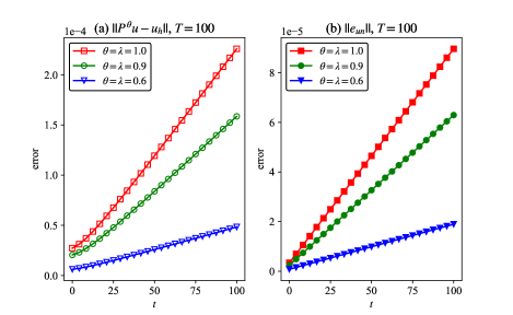
The errors and orders for , , , and with generalized numerical fluxes and are shown in Tables 6.1–6.2. We can see that the errors of numerical fluxes and cell averages achieve th order, and the function value error achieve th (th) order at generalized (derivative) Radau points. Also, the error between GGR projection and numerical solution is of th order. This demonstrates that the results in Theorem 4.2 are valid. In addition, the time evolution of the error up to for Example 6.1 is given in Figure 6.1, from which we can see that, at least for and , the generalized fluxes ( and ) produce a slower error growth when compared with upwind and alternating fluxes ().
Example 6.2.
| Order | Order | Order | Order | ||||||
|---|---|---|---|---|---|---|---|---|---|
| 16 | 2.05E-04 | – | 7.85E-04 | – | 1.20E-03 | – | 3.10E-03 | – | |
| 32 | 1.40E-05 | 3.87 | 9.44E-05 | 3.05 | 1.56E-04 | 2.98 | 8.36E-04 | 1.90 | |
| 64 | 1.27E-06 | 3.47 | 1.17E-05 | 3.01 | 2.07E-05 | 2.91 | 2.13E-04 | 1.97 | |
| 128 | 1.37E-07 | 3.21 | 1.46E-06 | 3.00 | 2.67E-06 | 2.96 | 5.39E-05 | 1.98 | |
| 8 | 1.51E-05 | – | 2.34E-05 | – | 7.85E-05 | – | 2.80E-03 | – | |
| 16 | 1.90E-07 | 6.31 | 7.26E-07 | 5.01 | 7.40E-06 | 3.41 | 3.87E-04 | 2.88 | |
| 32 | 3.23E-09 | 5.88 | 2.19E-08 | 5.05 | 5.00E-07 | 3.89 | 4.94E-05 | 2.97 | |
| 64 | 1.03E-10 | 4.97 | 6.76E-10 | 5.02 | 4.15E-08 | 3.59 | 6.24E-06 | 2.99 | |
| 10 | 2.75E-08 | – | 3.75E-08 | – | 4.92E-06 | – | 6.68E-05 | – | |
| 15 | 1.63E-09 | 6.97 | 2.17E-09 | 7.02 | 6.41E-07 | 5.03 | 1.33E-05 | 3.97 | |
| 20 | 2.16E-10 | 7.02 | 2.87E-10 | 7.03 | 1.53E-07 | 4.99 | 4.22E-06 | 4.00 | |
| 25 | 4.56E-11 | 6.98 | 6.03E-11 | 6.99 | 5.05E-08 | 4.96 | 1.74E-06 | 3.96 |
Numerical errors and orders with generalized fluxes (, ) are provided in Table 6.3, illustrating that the theoretical results in Theorem 5.1 with mixed boundary conditions are true, even for .
| Order | Order | Order | Order | ||||||
|---|---|---|---|---|---|---|---|---|---|
| 16 | 1.30E-03 | – | 1.60E-03 | – | 3.40E-03 | – | 6.30E-03 | – | |
| 32 | 1.59E-04 | 3.00 | 2.02E-04 | 3.00 | 4.22E-04 | 3.01 | 1.20E-03 | 2.45 | |
| 64 | 1.03E-05 | 3.94 | 1.73E-05 | 3.55 | 3.12E-05 | 3.76 | 2.24E-04 | 2.37 | |
| 128 | 6.27E-07 | 4.04 | 1.71E-06 | 3.34 | 2.82E-06 | 3.47 | 5.44E-05 | 2.04 | |
| 8 | 1.43E-05 | – | 2.98E-05 | – | 1.08E-04 | – | 2.90E-03 | – | |
| 16 | 1.77E-07 | 6.33 | 7.73E-07 | 5.27 | 6.99E-06 | 3.95 | 3.87E-04 | 2.88 | |
| 32 | 1.47E-09 | 6.92 | 2.25E-08 | 5.10 | 4.94E-07 | 3.82 | 4.94E-05 | 2.97 | |
| 64 | 6.29E-11 | 4.55 | 6.90E-10 | 5.03 | 4.14E-08 | 3.58 | 6.24E-06 | 2.99 | |
| 10 | 3.20E-06 | – | 2.98E-06 | – | 9.03E-06 | – | 7.03E-05 | – | |
| 15 | 1.77E-07 | 7.13 | 1.70E-07 | 7.06 | 8.43E-07 | 5.85 | 1.34E-05 | 4.08 | |
| 20 | 2.31E-08 | 7.09 | 2.24E-08 | 7.05 | 1.76E-07 | 5.45 | 4.24E-06 | 4.00 | |
| 25 | 4.75E-09 | 7.08 | 4.65E-09 | 7.05 | 5.52E-08 | 5.19 | 1.74E-06 | 3.98 |
We also consider (6.1) with Dirichlet boundary conditions
| (6.4) |
where () are suitably chosen such that the exact solution is (6.2). The numerical fluxes are
| (6.5) |
where and are penalty parameters. In Table 6.4, we show superconvergence results for generalized fluxes with , and , , indicating that the superconvergent results are also valid for Dirichlet boundary conditions.
Example 6.3.
In the case of discontinuous initial value problem, we consider
with periodic boundary conditions. With negligible error, the exact solution is taken as that in [17], i.e.,
Superconvergent orders of numerical fluxes, cell averages and Radau points with , , are presented in Table 6.5. This demonstrates that superconvergent results also hold for discontinuous initial value problem.
| Order | Order | Order | Order | ||||||
|---|---|---|---|---|---|---|---|---|---|
| 8 | 9.78E-04 | – | 4.40E-04 | – | 1.60E-03 | – | 4.78E-02 | – | |
| 16 | 1.04E-04 | 3.24 | 2.77E-05 | 3.99 | 2.62E-04 | 2.63 | 1.43E-02 | 1.74 | |
| 24 | 2.97E-05 | 3.08 | 5.82E-06 | 3.85 | 8.12E-05 | 2.89 | 6.60E-03 | 1.91 | |
| 32 | 1.24E-05 | 3.04 | 2.08E-06 | 3.58 | 3.48E-05 | 2.95 | 3.70E-03 | 1.96 | |
| 12 | 1.32E-06 | – | 1.10E-07 | – | 2.51E-05 | – | 7.39E-04 | – | |
| 16 | 3.17E-07 | 4.97 | 2.41E-08 | 5.28 | 8.16E-06 | 3.91 | 3.14E-04 | 2.98 | |
| 20 | 1.04E-07 | 4.98 | 7.55E-09 | 5.19 | 3.38E-06 | 3.95 | 1.61E-04 | 2.99 | |
| 24 | 4.20E-08 | 4.99 | 2.95E-09 | 5.15 | 1.64E-06 | 3.97 | 9.34E-05 | 2.99 | |
| 4 | 4.16E-06 | – | 1.67E-06 | – | 1.51E-04 | – | 1.61E-02 | – | |
| 8 | 3.48E-08 | 6.90 | 7.88E-09 | 7.73 | 7.47E-06 | 4.34 | 1.40E-03 | 3.51 | |
| 12 | 2.20E-09 | 6.81 | 3.31E-10 | 7.82 | 1.10E-06 | 4.73 | 3.06E-04 | 3.77 | |
| 16 | 3.03E-10 | 6.89 | 3.54E-11 | 7.77 | 2.71E-07 | 4.86 | 1.01E-04 | 3.87 |
Example 6.4.
To investigate the case for nonlinear problems, consider the Kuramoto–Sivashinsky equation
with and the exact solution is
where , , and . Note that periodic boundary conditions can be used, as the boundary value is quite small for short time simulations, say .
We use the Godunov flux for the nonlinear convection term and generalized fluxes for linear terms. Table 6.6 lists superconvergent orders for numerical fluxes generalized fluxes with , , which shows that the superconvergence property also holds true for nonlinear problems.
| Order | Order | Order | Order | ||||||
|---|---|---|---|---|---|---|---|---|---|
| 160 | 1.60E-03 | – | 1.50E-03 | – | 1.43E-02 | – | 4.14E-02 | – | |
| 320 | 1.66E-04 | 3.27 | 1.97E-04 | 2.90 | 1.60E-03 | 3.19 | 1.23E-02 | 1.75 | |
| 480 | 4.59E-05 | 3.16 | 6.02E-05 | 2.92 | 4.53E-04 | 3.07 | 5.60E-03 | 1.92 | |
| 640 | 1.88E-05 | 3.11 | 2.58E-05 | 2.94 | 1.94E-04 | 2.94 | 3.20E-03 | 1.96 | |
| 120 | 5.82E-05 | – | 2.82E-05 | – | 5.27E-04 | – | 2.13E-02 | – | |
| 160 | 1.37E-05 | 5.02 | 6.97E-06 | 4.86 | 1.82E-04 | 3.70 | 9.37E-03 | 2.85 | |
| 200 | 4.45E-06 | 5.06 | 2.29E-06 | 4.98 | 7.20E-05 | 4.15 | 5.23E-03 | 2.61 | |
| 240 | 1.76E-06 | 5.07 | 9.13E-07 | 5.04 | 3.69E-05 | 3.67 | 2.99E-03 | 3.08 | |
| 40 | 1.19E-03 | – | 1.04E-03 | – | 2.19E-02 | – | 7.96E-02 | – | |
| 80 | 3.05E-06 | 8.61 | 5.35E-06 | 7.60 | 6.16E-04 | 5.15 | 6.85E-03 | 3.54 | |
| 120 | 1.55E-07 | 7.34 | 2.28E-07 | 7.78 | 8.75E-05 | 4.81 | 1.43E-03 | 3.86 | |
| 160 | 2.37E-08 | 6.53 | 3.08E-08 | 6.97 | 2.45E-05 | 4.43 | 5.44E-04 | 3.37 |
7 Concluding remarks
In this paper, we study superconvergence of the LDG method using generalized numerical fluxes for one-dimensional linear fourth-order problems. By constructing correction functions and using properties of GGR projections, a superconvergent bound for interpolation errors is shown. Under a suitable numerical initial condition, superconvergence regarding numerical flux, cell averages and generalized Radau points are established. Extension to mixed boundary conditions is given. Problems with Dirichlet boundary conditions, discontinuous initial condition and nonlinear convection term are also numerically tested, demonstrating that the superconvergence results hold for more general cases. Analysis of nonlinear and multidimensional equations is challenging, which constitutes our future work.
References
- [1] Susanne C Brenner, Poincaré–Friedrichs Inequalities for Piecewise Functions, SIAM Journal on Numerical Analysis 41 (2003), no. 1, 306–324.
- [2] John W Cahn and John E Hilliard, Free energy of a nonuniform system. I. Interfacial free energy, The Journal of Chemical Physics 28 (1958), no. 2, 258–267.
- [3] Waixiang Cao and Qiumei Huang, Superconvergence of local discontinuous Galerkin methods for partial differential equations with higher order derivatives, Journal of Scientific Computing 72 (2017), no. 2, 761–791.
- [4] Waixiang Cao, Dongfang Li, Yang Yang, and Zhimin Zhang, Superconvergence of discontinuous Galerkin methods based on upwind-biased fluxes for 1D linear hyperbolic equations, ESAIM: Mathematical Modelling and Numerical Analysis 51 (2017), no. 2, 467–486.
- [5] Waixiang Cao, Zhimin Zhang, and Qingsong Zou, Superconvergence of discontinuous Galerkin methods for linear hyperbolic equations, SIAM Journal on Numerical Analysis 52 (2014), no. 5, 2555–2573.
- [6] Yao Cheng, Xiong Meng, and Qiang Zhang, Application of generalized Gauss–Radau projections for the local discontinuous Galerkin method for linear convection-diffusion equations, Mathematics of Computation 86 (2017), no. 305, 1233–1267.
- [7] Bernardo Cockburn, Suchung Hou, and Chi-Wang Shu, The Runge–Kutta local projection discontinuous Galerkin finite element method for conservation laws IV: The multidimensional case, Mathematics of Computation 54 (1990), no. 190, 545–581.
- [8] Bernardo Cockburn and Chi-Wang Shu, TVB Runge–Kutta local projection discontinuous Galerkin finite element method for conservation laws II: General framework, Mathematics of Computation 52 (1989), no. 186, 411–435.
- [9] , The local discontinuous Galerkin method for time-dependent convection-diffusion systems, SIAM Journal on Numerical Analysis 35 (1998), no. 6, 2440–2463.
- [10] , The Runge–Kutta discontinuous Galerkin method for conservation laws V: multidimensional systems, Journal of Computational Physics 141 (1998), no. 2, 199–224.
- [11] Bo Dong and Chi-Wang Shu, Analysis of a local discontinuous Galerkin method for linear time-dependent fourth-order problems, SIAM Journal on Numerical Analysis 47 (2009), no. 5, 3240–3268.
- [12] Harsha Hutridurga, Krishan Kumar, and Amiya K Pani, Discontinuous Galerkin methods with generalized numerical fluxes for the Vlasov-Viscous Burgers’ system, Journal of Scientific Computing 96 (2023), no. 1, article no.7.
- [13] Jia Li, Dazhi Zhang, Xiong Meng, and Boying Wu, Analysis of local discontinuous Galerkin methods with generalized numerical fluxes for linearized KdV equations, Mathematics of Computation 89 (2020), no. 325, 2085–2111.
- [14] Hailiang Liu and Nattapol Ploymaklam, A local discontinuous galerkin method for the Burgers–Poisson equation, Numerische Mathematik 129 (2015), no. 2, 321–351.
- [15] Xiaobin Liu, Dazhi Zhang, Xiong Meng, and Boying Wu, Superconvergence of local discontinuous Galerkin methods with generalized alternating fluxes for 1D linear convection-diffusion equations, Science China Mathematics 64 (2021), no. 6, 1305–1320.
- [16] Yong Liu, Qi Tao, and Chi-Wang Shu, Analysis of optimal superconvergence of an ultraweak-local discontinuous Galerkin method for a time dependent fourth-order equation, ESAIM: Mathematical Modelling and Numerical Analysis 54 (2020), no. 6, 1797–1820.
- [17] Xiong Meng, Chi-Wang Shu, and Boying Wu, Superconvergence of the local discontinuous Galerkin method for linear fourth-order time-dependent problems in one space dimension, IMA Journal of Numerical Analysis 32 (2012), no. 4, 1294–1328.
- [18] , Optimal error estimates for discontinuous Galerkin methods based on upwind-biased fluxes for linear hyperbolic equations, Mathematics of Computation 85 (2016), no. 299, 1225–1261.
- [19] Yuqing Miao, Jue Yan, and Xinghui Zhong, Superconvergence study of the direct discontinuous Galerkin method and its variations for diffusion equations, Communications on Applied Mathematics and Computation 4 (2022), no. 1, 180–204.
- [20] Gerasimos Ntoukas, Juan Manzanero, Gonzalo Rubio, Eusebio Valero, and Esteban Ferrer, A free-energy stable p-adaptive nodal discontinuous Galerkin for the Cahn–Hilliard equation, Journal of Computational Physics 442 (2021), 110409.
- [21] Chi-Wang Shu, Discontinuous galerkin methods for time-dependent convection dominated problems: Basics, recent developments and comparison with other methods, Building bridges: connections and challenges in modern approaches to numerical partial differential equations (2016), 369–397.
- [22] Haijin Wang, Qiang Zhang, and Chi-Wang Shu, Implicit–explicit local discontinuous Galerkin methods with generalized alternating numerical fluxes for convection–diffusion problems, Journal of Scientific Computing 81 (2019), 2080–2114.
- [23] Yan Xu and Chi-Wang Shu, Local discontinuous galerkin methods for nonlinear Schrödinger equations, Journal of Computational Physics 205 (2005), no. 1, 72–97.
- [24] , Local discontinuous Galerkin methods for two classes of two-dimensional nonlinear wave equations, Physica D: Nonlinear Phenomena 208 (2005), no. 1-2, 21–58.
- [25] Jue Yan and Chi-Wang Shu, A local discontinuous Galerkin method for KdV type equations, SIAM Journal on Numerical Analysis 40 (2002), no. 2, 769–791.