Generalized volume-complexity for Lovelock black holes
Abstract
In this study, We explore the time dependence of the generalized complexity of Lovelock black holes via the ”complexity = anything” conjecture, which expands upon the notion of ”complexity = volume” and generates a large class of observables. By applying a specific condition, a more limited class can be chosen, whose time growth is equivalent to a conserved momentum. Specifically, we investigate the numerical full time behavior of complexity time rate, focusing on the second and third orders of Lovelock theory, incorporating an additional term -the square of the Weyl tensor of the background spacetime- into the generalization function. Furthermore, we study the case with three additional scalar terms: the square of Riemann and Ricci tensors, and the Ricci scalar for second-order gravity (GB) and show how it can affect to multiple asymptotic behavior of time. Additionally, we show how the phase transition of generalized complexity and its time evolution occur at point where the maximal generalized volume supersedes another branch. Moreover, we show the proportionality complexity time rate at late times to the difference of temperature times entropy in two horizons () for charged black holes, which can be corrected by a function of each radius in generalized case.
1 Introduction
In recent decades, the AdS/CFT correspondence has emerged as a powerful framework for investigating quantum gravity [1]. Moreover, quantum information theory has shed light on the theory of quantum gravity through this framework, for example, by quantities such as entanglement entropy and quantum complexity [2, 3]. Computational complexity, in the context of information theory, is defined as the minimum number of unitary quantum operators known as gates, that evolve an initial state into a final requiring state [4]. This notion has provided tools to study the complexity of CFT the in boundary, and gravitational theory in the bulk. The latter was led to CV, CA, and CV2.0 conjectures.
The CV conjecture, proposed within the AdS/CFT framework, is the first conjecture suggesting this physical quantity, motivated by ER=EPR [5], to justify the growth of the Einstein-Rosen Bridge (ERB) ”size” over time in an eternal AdS black hole, after the scrambling time [6] and the thermal equilibrium of dual boundary theories. Accordingly, the complexity can be quantified by the maximum volume of a hypersurface anchored in the boundary time slice (the spatial volume of ERB) where the boundary CFT state resides, expressed as [7, 8]
| (1) |
where is extremal hypersurface anchored in the boundary time slice .
In another attempt, CA conjecture was proposed that the complexity can be related to the action of a specific extremal surface in the bulk spacetime, so-called Wheeler-DeWitt (WDW) patch [9, 10]
| (2) |
In [11], authors define volume complexity for the Wheeler-DeWitt (WDW) patch as subregion complexity motivated by [12, 13], and propose CV2.0 conjecture of complexity as
| (3) |
There are some inherent ambiguities in the definitions of quantum complexity, such as choosing the reference state, adopting the unitary set of operators, and so on. Correspondingly, in the bulk theory, one expects there would be some freedom in introducing the holographic complexity. Recently, “generalized complexity” (or complexity = anything, CAny) conjecture has emerged as a generalized version of complexity in bulk, where complexity is not limited to a specific geometric quantity but can be described by a more general function [15, 14, 16]. This conjecture allows for a broader exploration of complexity measures beyond volume and action, giving rise to an unbounded class of new diffeomorphism-invariant observables. Such observables, which defined on codimension-one of bulk region, can be written as
| (4) |
where, is not necessarily equals to one, which led to the volume of hypersurface as in CV. Instead, it can be a general scalar function of bulk geometry, more precisely, metric and an embedding of the hypersurfaces. Furthermore, is codimension-one hypersurface in the bulk spacetime with boundary time slice . On the other hand, extremality of the hypersurface leads to
| (5) |
For simplicity, we follow the case , so the observable (4), denoted by generalized complexity , obeys above condition, so
| (6) |
where is the determinant of induced metric on the given hypersurface.
In the original literature of CAny conjecture [15, 14, 16] and other examples (e.g.[22, 23, 24, 25]), the authors specifically assumed
| (7) |
where is the Weyl tensor squared and corresponds to the CV prescription. There are also other assumptions like [16]. In this paper, we are going to study the generalized complexity of Lovelock’s theory as a generalization to Einstein gravity with higher curvatures. Our focus is on the second and third-order terms of the theory. In addition, in the case of Gauss-Bonnet gravity, we extend the assumption (7) to include four invariant terms in .
The remainder of this paper is organized as follows. In section 2, we review the generalized complexity proposal. In section 3, we briefly review Lovelock theory. Then, we numerically calculate the time dependence of the generalized complexity, specifically, for the second-order term of the theory (Gauss-Bonnet) and the third one, respectively in subsections 3.1 and 3.2. Section 4, corresponds to discussion about linear proportionality of complexity growth rate at late time to difference of multiplication temperature and entropy in two horizons, and how it can be corrected for the generalized case. Next, we show these arguments with numeric analyses for the cases considered in section 3. Finally, we conclude in section 5.
2 Generalized volume complexity
Here, we review the generalized volume complexity. The set-up includes a two-sided black hole with the dual field theory in boundary. The corresponding Penrose diagram is depicted schematically in Fig. 1. Boundary time is shown on both sides and their infinity. Dashed line in the middle shows minimum radius of spacetime that reaches zero in the top and bottom, which is the singularity in theory of gravity in bulk. Red dashed curves, on both sides near the border, show the maximum value of the radius. Also, the blue curve shows a hypersurface anchored at a specific time in the dual boundary theory.
For the Eddington-Finkelstein coordinates, metric is written as
| (8) |
where
| (9) |
and is -dimensional metric which can take spherical, planar and hyperbolic geometry, respectively, with as curvature. The generalized volume complexity as a codimension-one observable could be obtained from (6) and (7) as [15, 14, 16]
| (10) |
where dots indicate derivative with respect to , is volume of spatial spherical submanifold, and is given by plugging the background (8) in . Extremizing is equivalent to solving equations of motion when considering (10) as an action. Moreover, because spacetime is stationary, the momentum conjugate to coordinate is conserved
| (11) |
Since expression in (10) is invariant under reparametrization, one can fix parameter by choosing
| (12) |
Then it is straightforward to derive extremality conditions with two equations above as follows
| (13) | ||||
| (14) |
We can see the equation as of classical particle’s motion
| (15) |
with the effective potential as
| (16) |
The conserved momentum can be simply expressed as a function of turning point in the symmetric trajectory
| (17) |
On the other hand, by integrating (14), the conserved momentum would be fixed in terms of boundary time, which is in turn a function of turning point
| (18) |
As a result of symmetry, for coordinate in boundary and turning point we have
| (19) |
Further, integrating extremality relation of coordinate
| (20) |
Hence, one can show that is
| (21) |
Derivation of with respect to boundary time leads to
| (22) |
Now, we can study growth rate of generalized complexity by conserved momentum, which is related to the boundary time as both are functions of . Then, the late-time behavior of growth rate is determined by
| (23) |
where is local maximum of the
effective potential, and because at this radius time goes to infinity, it is known sometimes as ..
So for, stationary solutions of gravitational theories, analyzing time versus conserved momentum by (18) gives full time behavior of generalized complexity growth rate. Besides, for late time behavior replacing solutions of effective potential maxima in (23) is straightforward.
3 Lovelock theory
In this section, we review Lovelock theory of gravity. The Lagrangian in D=d+1 dimensions with negative cosmological constant and contribution of Maxwell field is given by [26, 28]
| (24) |
where is radius of AdS, are arbitrary coupling constants, and are Euler densities made by generalized Kronecker delta and Riemann tensors
| (25) |
where
| (26) |
The first and second terms in (24) refer to Einstein gravity Lagrangian and negative cosmological constant
| (27) |
respectively. The first two coupling constants of higher order terms
| (28) |
The static black holes solutions take the form [21]
| (29) |
We focus on spherical () black holes in this paper. We note that the above metric reads (8) in Eddington-Finkelstein coordinates.
In the following of this section, we focus on two simpler cases, second and third orders of theory and investigate their time dependence behavior of generalized complexity which is proportional to the conserved momentum.
3.1 AdS Gauss-Bonnet
For the second order of Lovelock gravity we have Gauss-Bonnet (GB) term as [21]
| (30) |
which has blackening function of the metric in form (29) or (8) for charged black hole as [21]
| (31) |
with
| (32) |
The ADM mass of the black hole in terms of inner and outer horizon radius - because of two horizons for charged black holes - and charge would be
| (33) |
One can calculate the Hawking’s temperature and Wald’s entropy as
| (34) |
| (35) |
We consider simpler case, five dimensional , so we get the square of Weyl tensor as
| (36) |
The Kretschmann scalar is
| (37) |
The square of Ricci tensor and Ricci scalar, which are non-constant for Lovelock spacetime geometry can be written respectively as
| (38) |
| (39) |
Now, by these scalar functions, we are going to build the generalization factor . We consider the following two cases:
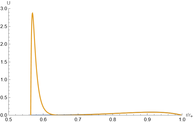
Case 1: We first consider the Weyl squared based factor as
| (40) |
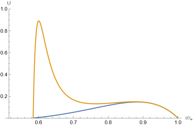
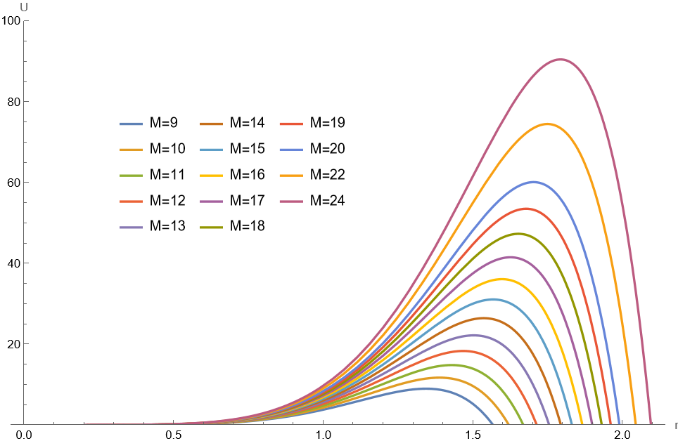
the effective potential behavior in terms of dimensionless parameter for this case is shown in Fig. 2LABEL:sub@fig:2a in comparison to i.e. when .
From (23), we know that any local maxima of the effective potential with radius results in infinite boundary time. The conserved momentum at each is known as . In this case, there are two peaks in comparison to one in .
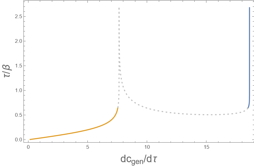
The numerical results of the boundary time versus , by (18) for (40) are shown in Fig. 2LABEL:sub@fig:2b. In all of calculations in this literature, is assumed.
The time equation integral yields real solutions for regions where slope of the diagram is negative in terms of radius and is greater than the next maximum. The numbers of these regions clearly depends on local maxima or points, with each peaks in the diagram be smaller than the previous one.
In the case, there is only one descending region from the maximum to the end. In contrast, for case, the effective potential have two peaks, and therefore two asymptotes appear in the diagram. The maximum points of momenta are denoted as and , referring to the left and right sides of the diagram. There are three branches in the diagram, two of which approach from the left and right, while the third one approaches from the right.
However, having different values of complexity rate at a single moment in time is not desirable. To determine the permissible intervals in each branch, another calculation for complexity as a function of boundary time is necessary.
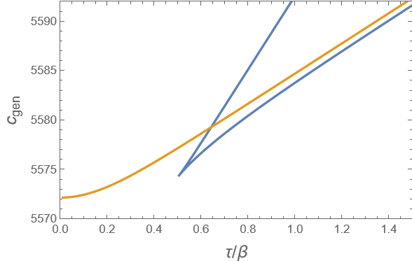
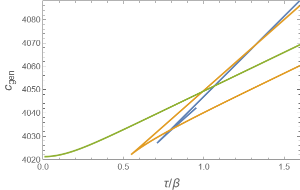
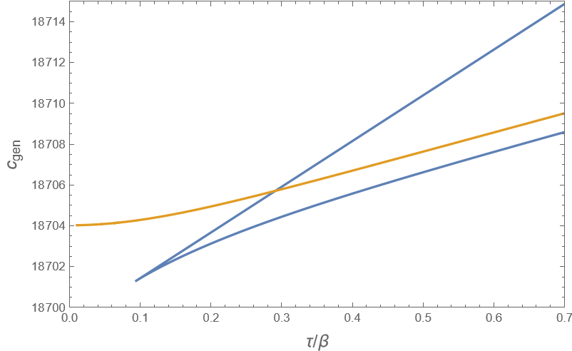
According to equation (10), a similar numerical computation of complexity as a function of radius can be applied. Subsequently, the results can be plotted against boundary time as depicted in Fig. 2LABEL:sub@fig:2c. We observe three branches, where the single branch and upper one in V-shaped curve are dipping. As defined in maximum volume complexity (see (6)), intervals with higher values are considered acceptable. Notably, at certain points, there are intersections of curves where maximal volume exchange occurs from one branch to another. These points in boundary time are referred to as , signifying a phase transition of complexity and its corresponding time growth (or equivalently, conserved momentum). In Fig. 2, the colors representing the complexity branches are consistent with those used to denote the allowed intervals before and after the phase transition in the diagram.
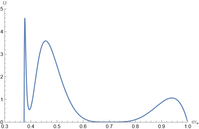
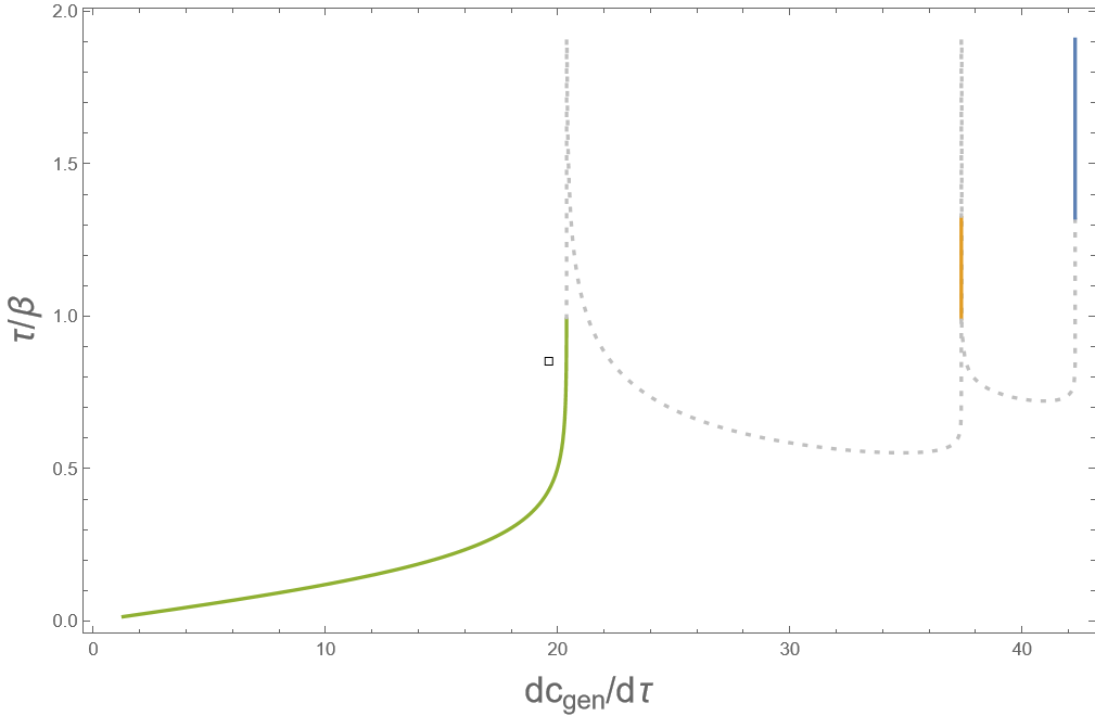
Case 2: One can see that more additive term in can result as extra maxima to the effective potential. For example we considered the case
| (41) |
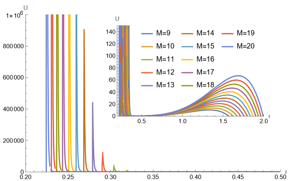
Such a factor can affect to potential as shown in Fig. 3LABEL:sub@fig:3a.
The boundary time (18) versus the is depicted in Fig. 3LABEL:sub@fig:3b. There are three peaks, with each peaks in the diagram be smaller than the previous one.
In this case with , in addition to left and right peaks, we have an extra peak are corresponds to in the middle, resulting three branches in diagram, approach to three ’s from left, and two branches approach and from right. The first three are named as dipping branches [15].
Similar to previous case, we performed a numerical computation of complexity versus the boundary time and depicted results in 3LABEL:sub@fig:3c. It can be seen that five branches show up from which the single branch and upper one in V-shaped curves are dipping. The phase transition points at where curves intersect each others and maximal volume jumps from one branch to another one.
It is worth noting that for three peaks in the effective potential and five complexity branches, other types of phase transitions, one or none at all, are possible. Examples of such scenarios can be found in [25].
3.2 Third order
Taking one step forward, we consider the third order term of theory [20, 27, 28] with Lagrangian
| (42) |
and blackening function for slowly rotating charged solution we have
| (43) |
where again
| (44) |
The ADM mass in terms of and charge would be
| (45) |
One can calculate the Hawking’s temperature and Wald’s entropy as
| (46) |
| (47) |
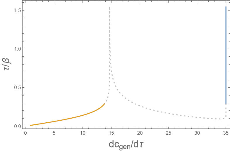
Here, we consider the case introduced in (40). For , the lowest dimensions of spacetime in which this term contributes, we get square of Weyl tensor as
| (48) |
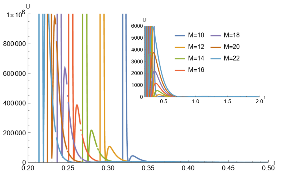
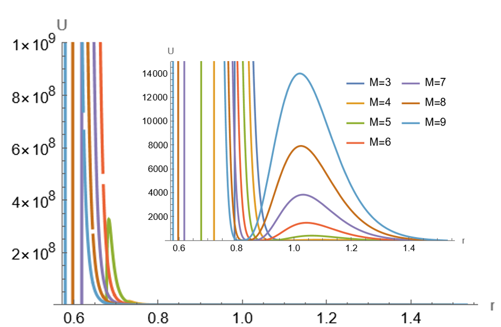
Regarding (40), the typical behavior of the effective potential in terms of dimensionless parameter for the third order Lovelock theory are shown in Fig. 4LABEL:sub@fig:4a. For the third order theory, similar to the GB case, adding Weyl squared term to , the number of maxima of the effective potential as a function of radius will increase to more than one. As discussed for GB, there are three branches for complexity growth rate due to two negative slope of potential, two of them approach to each from right, and the other approaches from left, which can be seen in boundary time versus the plot, Fig. 4LABEL:sub@fig:4b. Again, a third computation is done for complexity in time to find the phase transition point at . The corresponding diagram is depicted in Fig. 4LABEL:sub@fig:4c.
4 Late time behavior and thermodynamic quantities
As demonstrated in various literature, the growth rate of complexity in late times is directly proportional to temperature multiplied by entropy of the black hole (e.g. [21, 29, 30]).
| (49) |
For the black holes without charge and rotation, with one horizon, it equals to the ADM mass. For charged or rotating black holes which have two horizons, complexity growth rate usually is proportional to difference of in outer and inner horizons,
| (50) |
Moreover, in [14] it is argued that the proportionality to ADM mass is preserved for the generalized complexity. Here, we will investigate this feature for charged black holes for the volume and generalized complexity. To up-grate the proportionality relation (50) to the generalized complexity, it is expected that the right-hand side must be modified in some sort. Remember that Wald’s entropy can be introduced as a Noether’s charge from the Lagrangian density as follows [31, 32]:
| (51) |
where is binormal to the bifurcation surface. Promoting to the generalized complexity in (10), the volume element is replaced by , so one may consider the replacement of Lagrangian density as . Given the same binormals, then the partial derivation over Riemann tensor would be
| (52) |
It must be reminded that for complexity growth rate radius is , and at late time it reaches to event horizons (see Fig. 1). So, goes to zero and second term in (52) doesn’t contribute to the entropy. Hence, it inspires that for generalized complexity at late time, proportionality to difference of in outer and inner horizons should be corrected by multiplying generalization function in each horizon
| (53) |
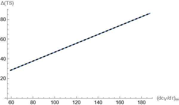
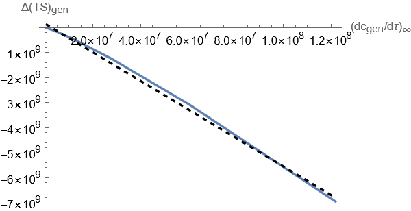
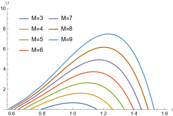
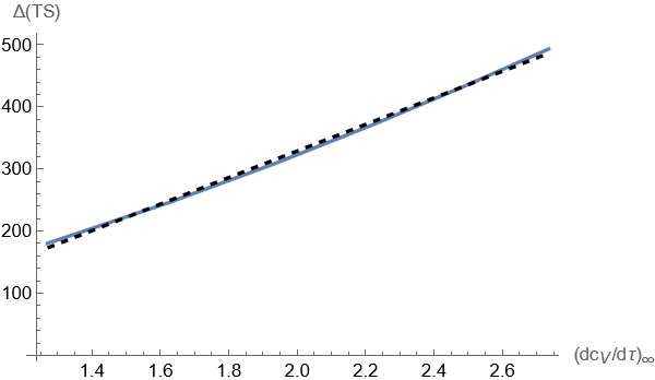
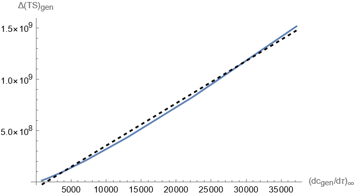
To verify these assertions, we performed the computations for three examples: i) GB with generalized complexity with Weyl tensor squared, ii) GB with three-term generalization functions, and iii) third order Lovelock with Weyl tensor squared. The numerical results are shown in Fig. 5 for GB in volume complexity cases i and ii, and in Fig. 6 for third order in volume complexity case iii. The left panel plots show the effective potentials of each case for different ADM masses, which can be directly calculated by their largest maxima complexity growth rate in late time. It is evident that in all cases for volume complexity (i.e. ) late time values are linear with the difference of in outer and inner horizons as (50), and for generalized cases, the numerical results are approximately in agreement with the modified linearity relation in (53).

5 Conclusion
In summary, the study presented in this paper explored the time dependence of generalized complexity in the context of Lovelock gravity, which extends Einstein’s theory by incorporating higher curvature terms. Specifically, we focused on two terms of the theory, the second order (GB) in 5 dimensions and the third one in 7. Our investigation centered on the time evolution of time growth rate of codimension-one generalized complexity () via conserved momentum conjugate to the coordinate in Eddington-Finkelstein coordinates, under the condition of equal and .
We used the generalization functions (40) and (41). For the first term, associated with the mode, a peak emerges in the effective potential or, similarly, conserved momentum diagram over the dimensionless radial quantity . Adding other terms led to the appearance of two or three peaks, referred to as . The numerical analysis of boundary time in terms of complexity growth rate revealed asymptotes at these points, and we studied the complexity against boundary time to determine the allowed branches. The maximal generalized volumes, defining the generalized complexity, were identified as the highest value intervals in these diagrams. Additionally, by computing the intersection points of different generalized volume curves, we identified times at which one maximal curve superseded another (i.e., ). Consequently, we observed certain parts of dipping branches approaching late-time asymptotes from the right, elucidating how phase transitions occur at .
Moreover, our numerical study in late time behavior of volume complexity time growth rate for charged Lovelock black holes revealed the linear relationship to difference of in outer and inner horizons. We deduced multiplying generalized function in each horizon to this thermodynamic quantity as a correction for generalized case. The following numerical results showed good approximation confirmation.
Acknowledgment
We would like to express our appreciation to Xuanha Wang and Yu-Xiao Liu for their invaluable guidance on conceptual aspects of this study. We also extend our thanks to Ghadir Jafari and Shan-Ming Ruan for providing technical support. Additionally, we are grateful to Reza Fareghbal, Ali Naseh, and Mojtaba Shahbazi for their constructive comments.
References
- [1] J. Maldacena, ”The Large N Limit of Superconformal Field Theories and Supergravity”, Adv.Theor.Math.Phys.2 (1998) 231-252, arXiv:9711200 [hep-th].
- [2] S. Ryu and T. Takayanagi, ”Holographic Derivation of Entanglement Entropy from AdS=CFT”, Phys. Rev. Lett. 96 (2006) 181602, arXiv:0603001 [hep-th]
- [3] M. Van Raamsdonk, ”Building up spacetime with quantum entanglement”, Gen.Relativ.Gravit. 42 (2010) 2323, Int. J. Mod. Phys. D 19 (2010) 2429 .
- [4] L. Susskind, ”Computational complexity and black hole horizons”, Fortsch.Phys. 64 (2016) 44-48 (addendum), Fortsch.Phys. 64 (2016) 24-43, arXiv:1403.5695 [hep-th], arXiv:1402.5674 [hep-th]
- [5] J. Maldacena and L. Susskind, ”Cool horizons for entangled black holes”, Fortsch.Phys. 61 (2013) 781-811, arXiv:1306.0533 [hep-th].
- [6] Y. Sekino and L. Susskind, ”Fast Scramblers”, JHEP 10 (2008) 065, arXiv: 0808.2096 [hep-th]
- [7] L. Susskind, ”Computational complexity and black hole horizons”, Fortsch.Phys. 64 (2016) 44-48 (addendum), Fortsch.Phys. 64 (2016) 24-43, arXiv:1403.5695 [hep-th], arXiv:1402.5674 [hep-th]
- [8] D. Stanford and L. Susskind, ”Complexity and Shock Wave Geometries”, Phys.Rev.D 90 (2014) 12, 126007, arXiv: 1406.2678 [hep-th]
- [9] A. R. Brown, D. A. Roberts, L. Susskind, B. Swingle, and Y. Zhao, ”Holographic Complexity Equals Bulk Action?”, Phys.Rev.Lett. 116 (2016) 19, 191301, arXiv: 1509.07876 [hep-th]
- [10] A. R. Brown, D. A. Roberts, L. Susskind, B. Swingle, and Y. Zhao, ”Complexity, action, and black holes”, Phys.Rev.D 93 (2016) 8, 086006, arXiv: 1512.04993 [hep-th]
- [11] J. Couch, W. Fischler and P.H. Nguyen, ”Noether charge, black hole volume, and complexity”, JHEP 03 (2017) 119, arXiv:1610.02038 [hep-th].
- [12] M. Alishahiha, ”Holographic Complexity”, Phys. Rev. D 92 (2015) 126009 arXiv:1509.06614 [hep-th].
- [13] O. Ben-Ami and D. Carmi, On Volumes of Subregions in Holography and Complexity, JHEP 11 (2016) 129 arXiv:1609.02514 [hep-th].
- [14] A. Belin et al., ”Does Complexity Equal Anything?”, Phys.Rev.Lett. 128 (2022) 8, 081602, arXiv:2111.02429 [hep-th].
- [15] A. Belin et al., ”Complexity equals anything II”, J. High Energy. Phys. 01 (2023) 154, arXiv:2210.09647 [hep-th].
- [16] E. Jørstad, R.C. Myers, and Ruan, SM. ”Complexity=anything: singularity probes”, J. High Energy. Phys. 7 (2023) 223, arXiv: 2304.05453 [hep-th].
- [17] D. Carmi, S. Chapman, H. Marrochio, R. C. Myers, and S. Sugishita, ”On the time dependence of holographic complexity”, J. High Energy Phys. 11 (2017) 188, arXiv: 1709.10184 [hep-th].
- [18] D. Carmi, S. Chapman, H. Marrochio, R. C. Myers, and S. Sugishita, ”On the time dependence of holographic complexity”, J. High Energy Phys. 11 (2017) 188, arXiv: 1709.10184 [hep-th].
- [19] M. Alishahiha, ”On complexity of Jackiw–Teitelboim gravity”, Eur.Phys.J.C 79 (2019) 4, 365, arXiv:1811.09028 [hep-th].
- [20] Z.Y. Fan, and H.Z. Liang, ”Time dependence of complexity for Lovelock black holes,” Phys.Rev.D 100 (2019) 8, 086016, arXiv:1908.09310 [hep-th].
- [21] Y.S. An, R.G. Cai, Y. Peng, ”Time Dependence of Holographic Complexity in Gauss-Bonnet Gravity”, Phys.Rev.D 98 (2018) 10, 106013, arXiv:1805.07775 [hep-th].
- [22] F. Omidi, Farzad, ”Generalized volume-complexity for two-sided hyperscaling violating black branes”, JHEP 01 (2023) 105, arXiv:2207.05287 [hep-th].
- [23] M.T. Wang, H.Y. Jiang, and Y.X. Liu, ”Generalized volume-complexity for RN-AdS black hole”, JHEP 07 (2023) 178, arXiv:2304.05751 [hep-th].
- [24] X. Wang, R. Li, and J. Wang, ”Generalized Volume Complexity in Gauss-Bonnet Gravity: Constraints and Phase Transitions”, arXiv:2307.12530 [hep-th].
- [25] M. Zhang, J.L. Sun, R.B. Mann, ”Generalized volume complexity of AdS rotating black holes”, arXiv:2401.08571 [hep-th].
- [26] D. Lovelock, ”The Einstein tensor and its generalizations”, J. Math. Phys. 12 (1971) 498-501.
- [27] M. H. Dehghani and R. Pourhasan, ”Thermodynamic instability of black holes of third order Lovelock gravity”, Phys. Rev. D 79 (2009) 064015, arXiv:0903.4260[hep-th].
- [28] M. H. Dehghani and M. Shamirzaie, ”Thermodynamics of asymptotic flat charged black holes in third order Lovelock gravity”, Phys. Rev. D 72 (2005) 124015, arXiv:0506227 [hep-th]
- [29] Z. Y. Fan, and M. Guo, ”Holographic complexity and thermodynamics of AdS black holes”, Phys. Rev. D, 100 (2019) 026016, arXiv:1903.04127 [hep-th] year = ”2019
- [30] D. Carmi, S. Chapman, H. Marrochio, et al., ”On the time dependence of holographic complexity”. J. High Energ. Phys. 188 (2017), arXiv:1709.10184 [hep-th]
- [31] R. M. Wald, ”Black hole entropy is the Noether charge”, Phys. Rev. D 48 (1993) 3427-3431, arXiv:9307038[gr-qc]
- [32] V. Iyer and R. M. Wald, ”Some properties of Noether charge and a proposal for dynamical black hole entropy”, Phys. Rev. D 50 (1994) 846-864, arXiv:9403028[gr-qc]