On the Impact of Bounded Rationality in Strategic Data Gathering
Abstract
We consider the problem of estimation from survey data gathered from strategic and boundedly-rational agents with heterogeneous objectives and available information. Particularly, we consider a setting where there are three different types of survey responders with varying levels of available information, strategicness, and cognitive hierarchy: i) a non-strategic agent with an honest response, ii) a strategic agent that believes everyone else is a non-strategic agent and that the decoder also believes the same, hence assumes a naive estimator, i.e., level-1 in cognitive hierarchy iii) and strategic agent that believes the population is Poisson distributed over the previous types, and that the decoder believes the same. We model each of these scenarios as a strategic classification of a 2-dimensional source (possibly correlated source and bias components) with quadratic distortion measures and provide a design algorithm. Finally, we provide our numerical results and the code to obtain them for research purposes at https://github.com/strategic-quantization/bounded-rationality.
Index Terms:
Behavioral sciences, Game theory, Bayesian estimation, Mathematical models, Human behavior modelingI Introduction
Consider the following scenario involving a survey designed to gauge public reception of a new plastic product, with responses influenced by respondents’ attitudes toward climate change. Respondents’ scores range from 1 (‘will definitely not use’) to 4 (‘will definitely use’), and the survey needs to account for potential biases as well as varying levels of rationality among respondents. We model this problem using the hierarchical cognitive type model as studied by [Camerer et al.(2004)Camerer, Ho, and Chong], considering three types of respondents:
-
•
Type 0 (Honest-Nonstrategic Respondents): These respondents provide truthful information based on their actual opinions about the product, unaffected by their considerations of climate change or any desire to bias the survey.
-
•
Type 1: These respondents wish to influence the survey outcome correlated with their attitudes. They best respond to Type 0, assuming that
-
1.
All other respondents are of Type 0.
-
2.
The estimator (designer) is only aware of Type 0 respondents.
-
1.
-
•
Type 2: These respondents have a higher level of strategic thinking and behave as the best response to a mix of Types 0 and 1, assuming that the designer (estimator) perceives the responses as coming from a distribution of these lower types.
The designer of the survey is aware of the existence of these types of respondents as well as their true statistics. The question explored in this paper is: What is the designer’s optimal “de-biasing” procedure, i.e, optimally (in Bayesian sense) estimating the unbiased scores that reflect the true public reception of the plastic product?
We approach this problem via the recently introduced strategic quantization framework, see [Akyol and Anand(2023)], which is a special case of the information design problem in Economics.111Throughout the paper, we use the terms quantizer and classifier interchangeably.This class of problems, notable studied by [Rayo and Segal(2010), Kamenica and Gentzkow(2011)] explore the use of information by an agent (sender) to influence the action taken by another agent (receiver), where the aforementioned action determines the payoffs for both agents. Our prior work explored strategic quantization problem settings where the sender and the receiver were assumed to be fully rational agents. In this paper, we extend our strategic quantization work to settings with boundedly-rational sender (quantizer), via employing the cognitive hierarchy model of [Camerer et al.(2004)Camerer, Ho, and Chong].
Throughout this paper, we focus on the quadratic distortion measures. Particularly, the senders observe a two-dimensional source with a known joint density function over and , where and can be interpreted as the state and bias variables. There are two types of strategic senders, both trying to minimize , with different assumptions on the estimator (receiver). Type 1 strategic users assume the estimator is simply nonstrategic (which is the best response to Type 0). Type 2, in turn, assumes that the decoder is aware of a mix of Type 0 and Type 1 senders.
The receiver’s objective is to estimate the true state in the minimum mean squared error (MME) sense, i.e., the receiver minimizes by choosing an action which is the optimal MMSE estimate of given the quantization index from the sender , hence . In sharp contrast with the conventional quantization problem where the sender chooses that minimizes , in this setting the sender’s choice of quantization mapping minimizes a biased estimate, i.e., . The objectives and the source distribution are common knowledge, available for all agents. We note that similar signaling problems with quadratic measures have been analyzed in the Economics literature, see e.g., [Crawford and Sobel(1982), Fischer and Verrecchia(2000), Bénabou and Tirole(2006)].
This paper is organized as follows: In Section II we present the problem formulation. In Section III, we present a gradient-descent based algorithm to compute the classifier implemented by the boundedly rational agent. We provide numerical results in Section IV, and conclude in Section V.

II Preliminaries
II-A Notation
In this paper, random variables are denoted using capital letters (say ), their sample values with respective lowercase letters (), and their alphabet with respective calligraphic letters (). Vectors are denoted in bold font. The set of real numbers is denoted by . The alphabet, , can be finite, infinite, or a continuum, like an interval . The 2-dimensional jointly Gaussian probability density function with mean and respective variances with a correlation is denoted by , . The expectation operator is written as . The operator denotes the absolute value if the argument is a scalar real number and the cardinality if the argument is a set.
III Problem Formulation
Consider the following classification problem: Three classifiers (senders), each with a probability of being chosen to send the message observe realizations of the two sources , with joint probability density . The chosen classifier maps to a message , where is a set of discrete messages with a cardinality constraint using a non-injective mapping . After receiving the message , the receiver applies a mapping on the message and takes an action .
The set is divided into mutually exclusive and exhaustive sets by each classifier as . Let the marginal probability density function of be .
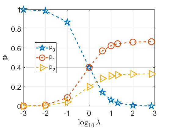
The probability of sender being chosen follows a normalized Poisson distribution
| (1) |
The distortion of the senders are , that of sender is , and that of the receiver is . Let be the estimate that assumes are optimized by the receiver with respect to the respective perceived receiver distortion , obtained by enforcing KKT conditions of optimality, . We consider three senders with hierarchical cognitive types and define the senders’ and their respective perceived receiver distortions as below:
-
1.
Non-strategic sender : similar to level cognitive type, the sender assumes all senders are of type , and that the decoder assumes all senders are of type . Sender considers the receiver’s distortion as the same as the sender’s, (provides the information required by the receiver honestly)
-
2.
Level-1 strategic sender : similar to level cognitive type, the sender assumes all other senders are of type and that it is uniquely of type . The sender assumes the receiver thinks that all sender types are , i.e., , which results in the estimates perceived by , .
-
3.
Level-2 strategic sender : similar to level cognitive type, the sender assumes the other senders are of lower cognitive levels and are Poisson distributed with a probability mass function ,
for , respectively. Note that this perceived probability mass function is not the actual statistics of the population, . The sender assumes the receiver is aware only of the types and and its perceived probability mass function and . Sender ’s perceived receiver distortion,
The encoder distortions for each type ,
The receiver’s distortion is given by
and that minimizes the above expression is the actual receiver’s action, .
Each sender type optimizes their classifiers with respect to their own distortion , assuming the receiver is aware of only sender types. Sender designs ex-ante, i.e., without the knowledge of the realization of , using only the objectives and , and the statistics of the source .
The receiver is fully rational and has full information about the classification setup. The shared prior (), the probability mass function over the sender types () and the mappings () are known to the receiver. The problem is to design the classifiers for the equilibrium, i.e., each sender type minimizes its own objective, assuming that the receiver minimizes its corresponding perceived objective . This classification problem is given in Fig. 1. Since the senders choose the classifiers first, followed by the receiver choosing the perceived estimates (), we look for a Stackelberg equilibrium.
The classifier design involves computing classifiers for each realization of by classifier as , where . Throughout this paper, we make the following “monotonicity” assumption on the sets .
Assumption 1
is convex for all .
That is, . Then, , where .
Since ’s distortion function is not a function of , simplifies to . Let for all . responds honestly, (equivalent to the non-strategic classification setting), hence its classifier and perceived estimates are,
assumes that all other senders are of type and that the receiver views all senders as type , i.e., ’s perceived estimates , since .
assumes the other agents are of types and with probability mass function , and that the receiver perceives the agents as the same, of types with a probability mass function ,
resulting in ’s perceived estimates ,
| (2) |
The classifier distortions for are given by
| (3) |
The receiver’s distortion and estimates are
| (4) |
| (5) |
The classifers implemented by are as follows:
-
1.
implements a non-strategic (classical) classifier for the given density of , .
-
2.
implements a nearest neighbor classifier for with respect to . Since assumes that the receiver views all senders as type , the estimates perceived by is the non-strategic estimates . Minimizing with estimates results in a nearest neighbor classifier, which is the non-strategic classifier shifted by for each realization , .
- 3.
IV Design
In this section, we present our gradient-descent based algorithm for the optimization of .
In [Anand and Akyol(2024)], we proposed a gradient-descent based algorithm to solve the problem of quantization of a 2-dimensional source by extending our algorithm in [Akyol and Anand(2023)] for a scalar source to the 2-dimensional setting by a simple method of computing quantizers for each value of .
Here, we use similar methods as in [Anand and Akyol(2024)], also using the known classifiers for , we perform gradient descent optimization with the objective as optimized over , assuming the estimates are optimized for . Although the sender’s objective depends on receiver estimates , since is a function of , the optimization can be implemented as a function of solely .
(a)
(b)
(c)
Parameters:
Input:
Output: , , , ,
Initialization: assign a set of monotone randomly, compute associated sender distortion , set iteration index ;
while or until a set amount of iterations do
Like any gradient-descent-based algorithm, the proposed method may get stuck at a poor local optimum, which we resolve with a simple remedy by performing gradient descent with multiple initializations and choosing the best local optimum among them. A sketch of the proposed method is summarized in Algorithm 1. The MATLAB codes are provided at https://github.com/strategic-quantization/bounded-rationality for research purposes.
V Numerical Results
We consider a jointly Gaussian 2-dimensional source
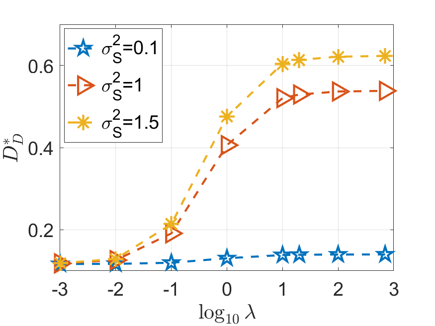
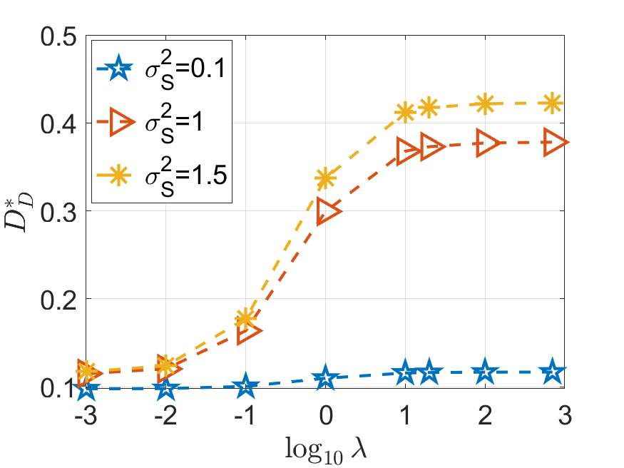
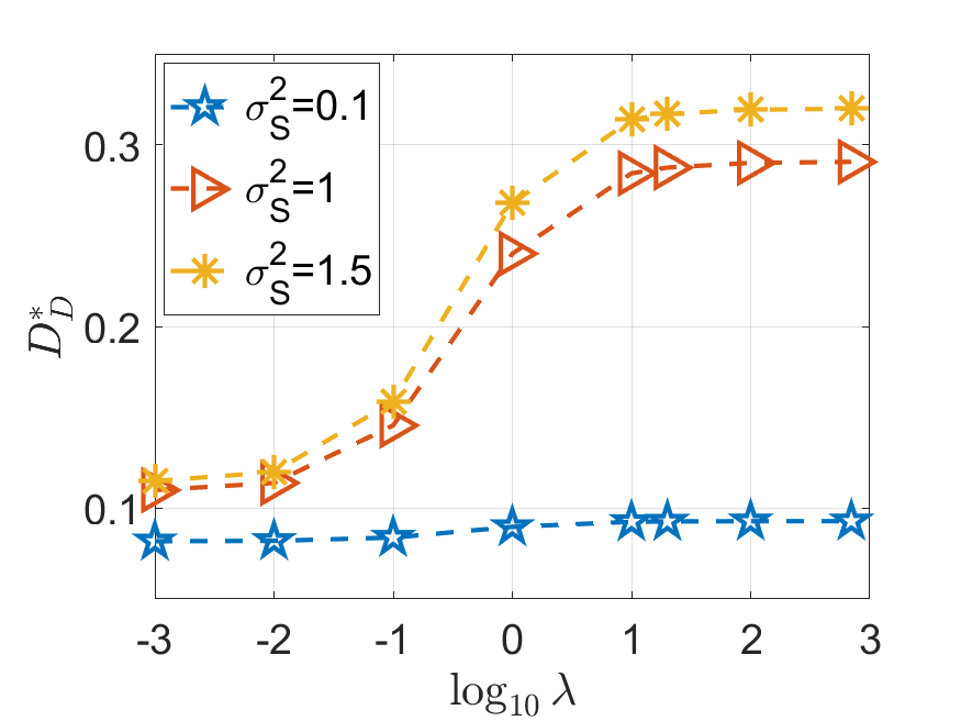
and present results for different settings with parameters bias variance , correlation , and following (1) with for an classifier. The probability mass function over the sender types for different values of is plotted in Fig. 2. We consider only positive correlation since people’s preferences are positively correlated with their opinions; for instance, both climate activists and climate change deniers try to bias their classification towards the extremes on their side. We plot the receiver’s distortion in Fig. 3 for given values of and , respectively.
We now interpret our results in terms of the impact of different parameters on the receiver’s estimation.
We observe from Fig. 3 that the correlation between the state and bias variables does not change the receiver distortion trends.
V-A Impact of cognitive parameter
From Fig. 2 we note that as , the population mostly consists of level-0 cognitive level. As increases, the population shifts towards higher cognitive types, and we expect the receiver distortion to increase with , as we observe in Fig. 3. For , the receiver distortion does not change significantly with varying bias variance since the population is mostly of level-0 type, and they respond honestly. For , the statistics of the population remain fairly constant, and hence the receiver distortion varies negligibly.
V-B Impact of varying
For a given correlation , we observe in Fig. 3 that as decreases, the receiver distortion decreases. As the variance of the bias decreases, the sender’s opinions are closer to their true value, and the objectives of the sender and the receiver become more aligned.
When the bias is negligible (), the objectives of all the senders are similar, resulting in a negligible change in the receiver distortion with , which we observe in Fig. 3 for .
V-C Comparison with different types of senders
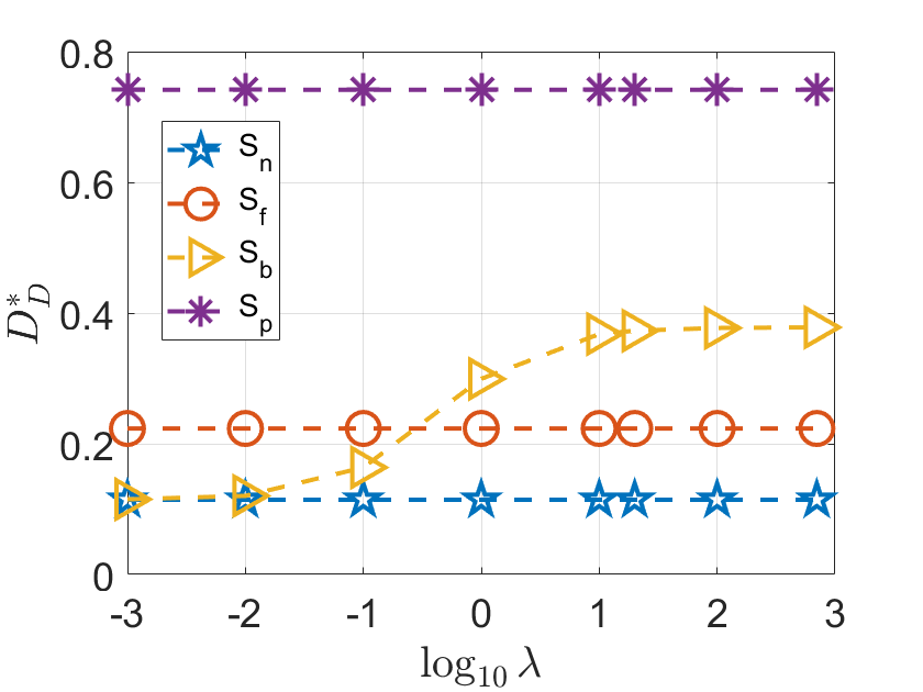
In Fig. 4, the receiver distortion for the following four different types of senders is plotted for a specific setting with :
-
1.
non-strategic (): All agents are non-strategic and send their honest reply ().
-
2.
full information (): All agents are fully rational and have full information. The classifier here is that in [Anand and Akyol(2024)].
-
3.
bounded rational (): The agents follow the setting described in this paper.
-
4.
partially-strategic (): All agents minimize , but they assume the receiver is not strategic and hence implements a naive estimator, . The classifier is the same as that for .
The receiver is fully rational with full information about the type of sender, the source distribution, and sender and receiver objectives.
As expected, the non-strategic sender results in the lowest receiver distortion. For negligible , the population is mostly of level-0 cognitive type, as mentioned before. Since they respond honestly, is closer to the non-strategic value as .
Although we expect that results in maximizing the receiver distortion among the above four senders, we observe from Fig. 4 that the receiver may prefer a fully rational sender with full information to other types of strategic senders for for some . We observe that the receiver benefits from a boundedly or fully rational setup compared to the setting where all senders are partially-strategic.
VI Conclusions
In this paper, we analyzed the problem of strategic classification of a 2-dimensional source with three types of senders with hierarchical cognitive types: level-0 non-strategic, level-1 strategic, and level-2 strategic, where each level assumes they are unique and that the other agents have lower cognitive levels. We considered quadratic objectives for the sender and the receiver and extended our prior work on design, a gradient-descent based algorithm for a 2-dimensional source with a single type of fully rational sender with full information, to the bounded-rational setting considered in this paper. The numerical results obtained via the proposed algorithm suggest several intriguing research problems that we leave as a part of our future work.
References
- [Akyol and Anand(2023)] Akyol, E. and Anand, A. (2023). Strategic Quantization. In IEEE International Symposium on Information Theory (ISIT), 543–548.
- [Anand and Akyol(2024)] Anand, A. and Akyol, E. (2024). Strategic Quantization with Quadratic Distortion Measures. In https://tinyurl.com/CPHS2024-bounded-rationality, Working Paper.
- [Bénabou and Tirole(2006)] Bénabou, R. and Tirole, J. (2006). Incentives and Prosocial Behavior. American Economic Review, 96(5), 1652–1678.
- [Camerer et al.(2004)Camerer, Ho, and Chong] Camerer, C.F., Ho, T.H., and Chong, J.K. (2004). A Cognitive Hierarchy Model of Games. The Quarterly Journal of Economics, 119(3), 861–898.
- [Crawford and Sobel(1982)] Crawford, V.P. and Sobel, J. (1982). Strategic Information Transmission. Econometrica: Journal of the Econometric Society, 1431–1451.
- [Fischer and Verrecchia(2000)] Fischer, P.E. and Verrecchia, R.E. (2000). Reporting Bias. The Accounting Review, 75(2), 229–245.
- [Kamenica and Gentzkow(2011)] Kamenica, E. and Gentzkow, M. (2011). Bayesian Persuasion. American Economic Review, 101(6), 2590–2615.
- [Rayo and Segal(2010)] Rayo, L. and Segal, I. (2010). Optimal Information Disclosure. Journal of Political Economy, 118(5), 949–987.