Chiral and topological superconductivity in isospin polarized multilayer graphene

Abstract

A microscopic mechanism for chiral superconductivity from Coulomb repulsion is proposed for spin- and valley-polarized state of rhombohedral multilayer graphene. The superconducting state occurs at low density, has chiral $p$-wave pairing symmetry, and exhibits highest $T_{c}$ close to a Lifshitz transition from annular to simply-connected Fermi sea. This Lifshitz transition also marks a topological phase transition from a trivial to a topological superconducting phase hosting Majorana fermions. The chirality of the superconducting order parameter is selected by the chirality of the valley-polarized Bloch electrons. Our results are in reasonable agreement with observations in a recent experiment on tetralayer graphene [arXiv:2408.15233 [1]].

Chiral superconductivity, characterized by spontaneous time-reversal symmetry breaking and finite-angular momentum Cooper pairing [2], is a long-sought quantum phase of matter with unusual superconducting and magnetic properties. Interest in chiral superconductors is further fueled by their potential for hosting topological phases and Majorana fermions [3, 4]. While previous material candidates, such as ${\rm Sr}_{2}{\rm RuO}_{4}$ [5] and ${\rm UTe}_{2}$ [6, 7, 8], showed initial signs of chiral superconductivity, recent experiments strongly suggest single-component superconducting order parameters that are non-chiral [9, 10, 11, 12, 13, 14, 15, 16].

Very recently, signatures of chiral superconductivity have been observed in rhombohedral-stacked tetralayer graphene under electron doping [1]. While superconductivity has been previously discovered and intensively studied in crystalline trilayer [17, 18, 19, 20, 21, 22, 23, 24, 25, 26, 27, 28, 29] and bilayer graphene [30, 31, 32, 33, 34, 35] , the newly found superconducting state in tetralayer graphene at low density is remarkably distinctive in that they exhibit large spontaneous anomalous Hall effect above $T_{c}$ and magnetic hysteresis in resistance below $T_{c}$. These observations demonstrate time-reversal-breaking superconductivity in a pure carbon system. Its pairing symmetry and pairing mechanism are open questions for investigation.

A key feature of rhombohedral multilayer graphene is the flat band dispersion near $K$ and $K^{\prime}$ points leading to strong correlation effect [19, 23]. As a result, spin and valley isospin symmetry breaking occurs at low temperature, giving rise to half and quarter metal phases [23]. Interestingly, the superconducting state in tetralayer graphene at low density borders the quarter metal and their phase boundary shows no or little change with the applied magnetic field, indicating that the superconducting state is likely fully spin and valley polarized [1]. Thus, tetralayer graphene provides a rare opportunity for investigating Cooper pairing of single flavor electrons in a solid state platform.

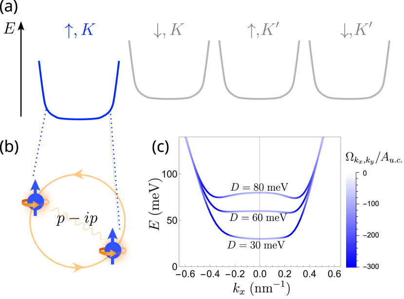
Figure 1: (a) Schematic of a chiral superconducting pairing appearing on top of an isospin-polarized quarter-metal state in multilayer graphene. (b) The chirality of the superconducting state is selected by the orbital magnetic moment of the electrons in the polarized valley. (c) Dispersion of ABCA graphene around the $K$ valley [19, 23] for various electric potential differences $D$ between top and bottom layers. The line color indicates the Berry curvature $\Omega_{k_{x},k_{y}}$.

In this work, we study microscopic mechanism and pairing symmetry of superconductivity in multilayer graphene that develops from the spin- and valley-polarized quarter metal normal state. Our mechanism is based on the overscreening of Coulomb interaction due to charge fluctuations, which leads to an effective attraction at length scales of a few Fermi wavelengths driving Cooper pairing . Using a minimal model for the band dispersion, our theory predicts that superconductivity occurs at low densities with enhanced density of states due to the annular Fermi surface and displacement field-induced flatness of the band.

In the spin- and valley-polarized state, the Pauli principle dictates that a Cooper pair can only be formed by two electrons having odd relative angular momentum, for example, with $p$- or $f$-wave symmetry [37]. Using Coulomb interaction and including the effect of dielectric screening in two dimensions, we find robust $p$-wave superconductivity at densities and temperatures in reasonable agreement with the experiment. The calculated $T_{c}$ is on the order between $100\,{\rm mK}$ to a few ${\rm K}$, depending on the dielectric screening of the Coulomb interaction in the graphene film relative to the surrounding dielectric. Relatedly, we find that electrons are paired even relatively far from the Fermi surface. Our results indicate that generally, a chiral $p-i\tau p$ ordering is favored ($\tau=\pm 1$ stands for $K/K^{\prime}$ valley, independent on spin polarization), and we predict a number of relevant experimental signatures for it.

Band dispersion.— In rhombohedral multilayer graphene, low-energy bands come from sublattice polarized states in the top and bottom layers. An out-of-plane electric field induces a potential bias equal to $2D$ between these layers and opens up an energy gap while flattening the dispersion near $K$ and $K^{\prime}$ points. Therefore, the Fermi energy is only a few ${\rm meV}$ above the band bottom for small electron density of around $5\times 10^{11}{\rm cm}^{-2}$, where time-reversal-breaking superconductivity is observed.

The low-energy band dispersion is highly tunable by the electric field. As $D$ increases, the curvature at $K$ and $K^{\prime}$ changes from positive to negative [19, 23] as shown in Fig. 1(c) for ABCA tetralayer graphene, resulting in a Mexican-hat shaped dispersion. In this case, a Lifshitz transition from simple to annular Fermi surface occurs as electron density is reduced.

We capture the essential features of the electric-field-tuned conduction band in rhombohedral $n$-layer graphene with a minimal band dispersion:

$$\varepsilon_{k}=D\sqrt{1+(k/k_{0})^{2n}}+\frac{\hbar^{2}k^{2}}{2m}$$ (1)

where we set $n=4$ corresponding to the tetralayer and treat $k_{0}$ and $m$ as fit parameters to approximate the $D$-dependent band dispersion of multilayer graphene , see App. A. The functional form of Eq. 1 is derived from an effective 2-band model of rhombohedral tetralayer graphene with nearest-neighbor hopping [39]. The dispersion (1) is circularly symmetric. The inclusion of additional hopping terms leads to trigonal warping. For now, we neglect trigonal warping and Berry curvature effects, and will treat them perturbatively later.

Rytova-Keldysh potential.— The density-density interaction can be written as

$$H_{int}=\frac{1}{2}\sum_{\bm{k},\bm{k}^{\prime},\bm{q}}V(\bm{q})\psi^{\dagger}_{\bm{k}+\bm{q}}\psi^{\dagger}_{\bm{k}^{\prime}-\bm{q}}\psi_{\bm{k}^{\prime}}\psi_{\bm{k}},$$ (2)

where $\psi^{(\dagger)}_{k}$ are the electron field annihilation (creation) operators. Importantly, in a 2D material surrounded by a dielectric with a lower dielectric permittivity, the Coulomb interaction between two charges can be described by the Rytova-Keldysh potential [40, 41, 42], taking the form:

$$V(\bm{q})=\frac{e^{2}}{2\epsilon|q|(1+r_{K}|q|)}$$ (3)

where $\epsilon=5\,\epsilon_{0}$ is the dielectric permittivity of the surrounding hBN (with $\epsilon_{0}$ the vacuum permittivity), and $r_{K}$ is the Rytova-Keldysh parameter. The Rytova-Keldysh parameter depends on the difference of the dielectric response of the 2D material under study relative to the surrounding insulator. Since the 2D dielectric screening depends on the band gap, $r_{K}$ of multilayer graphene is affected by the displacement field [43]. We will find that the superconducting pairing strength depends sensitively on $r_{K}$.

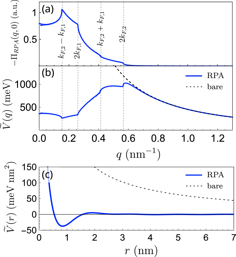
Figure 2: (a) Charge susceptibility of the non-interacting electron gas. (b), (c) Screened (solid line) and bare (dashed) Rytova-Keldysh interaction potential in momentum and real space, respectively.

Electron pairing from screened Coulomb repulsion.— Our mechanism for superconductivity is based on screening of electron-electron interactions [44, 45, 46]. The screening is described by the charge susceptibility $\chi_{e}^{{\rm R}}(\bm{q},\tau)=-\frac{1}{A}\langle T_{\tau}\rho_{e,\bm{q}}(\tau)\rho_{e,-\bm{q}}(0)\rangle$ which in random phase approximation (RPA) is determined by the expression

$$\chi_{e}^{{\rm R}}(\bm{q},i\Omega_{n})\overset{\rm RPA}{\approx}\frac{\chi_{e}^{{\rm 0R}}(\bm{q},i\Omega_{n})}{1-V_{\bm{q}}\chi_{e}^{{\rm 0R}}(\bm{q},i\Omega_{n})/e^{2}}$$ (4)

in terms of the charge susceptibility of the non-interacting electron gas

$$\chi_{e}^{{\rm 0R}}(\bm{q},i\Omega_{n})=\frac{e^{2}}{A}\sum_{\bm{k}}\frac{n_{F}(\varepsilon_{\bm{k}})-n_{F}(\varepsilon_{\bm{k}+\bm{q}})}{\varepsilon_{\bm{k}}-\varepsilon_{\bm{k}+\bm{q}}+i\hbar\Omega_{n}}$$ (5)

where $\tau$ is imaginary time and $i\Omega_{n}$ Matsubara frequencies. With the resulting dielectric response function $\epsilon^{-1}(\bm{q},\omega)=1+V_{\bm{q}}\chi_{e}^{{\rm R}}(\bm{q},\omega)/e^{2}$ one obtains the screened interaction potential

$$\tilde{V}_{\bm{q}}=V_{\bm{q}}\epsilon^{-1}(\bm{q},0)\overset{\rm RPA}{\approx}\frac{V_{\bm{q}}}{1-V_{\bm{q}}\chi_{e}^{{\rm 0R}}(\bm{q},\omega)/e^{2}}\,.$$ (6)

The charge susceptibility and screened interaction potential for the annular Fermi pocket are shown in Fig. 2(a) and (b), respectively.

Due to the large density of states, the charge susceptibility becomes large for momenta below twice the Fermi momentum $k_{F,2}$ of the outer Fermi surface. This leads to a suppression of the electron-electron interaction at small momenta and a peak at $2k_{F,2}$. The screening strongly reduces the repulsion on long length scales compared to the Fermi wavelength, and leads to an over-screening with an effective attraction at distances of a few Fermi wavelengths, as demonstrated in Fig. 2(c).

To determine the superconducting order parameter and its critical temperature, we solve the self-consistency equations

$$\Delta(\bm{k}) = \frac{1}{A}\sum_{\bm{k}^{\prime}}\tilde{V}(\bm{k}-\bm{k}^{\prime})\langle\hat{\psi}_{-\bm{k^{\prime}}}\hat{\psi}_{\bm{k^{\prime}}}\rangle,$$

$$\langle\hat{\psi}_{-\bm{k}}\hat{\psi}_{\bm{k}}\rangle = -\frac{\Delta(\bm{k})}{2E_{\bm{k}}}\tanh\frac{E_{\bm{k}}}{2k_{B}T},$$ (7)

where $E_{\bm{k}}$ is the quasiparticle energy

$$E_{\bm{k}}=\sqrt{(\varepsilon_{\bm{k}}-\mu)^{2}+|\Delta(\bm{k})|^{2}}.$$ (8)

Here the interaction $\tilde{V}(\bm{k}-\bm{k}^{\prime})$ scatters a pair of electrons at opposite momenta $(\bm{k}^{\prime},-\bm{k}^{\prime})$ to $(\bm{k},-\bm{k})$. Due to the rotational symmetry in our model, we decompose the pairing interaction into angular harmonics:

$$\tilde{V}_{l}(k,k^{\prime})\equiv\int_{0}^{2\pi}d\vartheta e^{il\vartheta}\tilde{V}(\vartheta,k,k^{\prime})$$ (9)

where we wrote $\tilde{V}_{\bm{k}-\bm{k}^{\prime}}=\tilde{V}(\vartheta,k,k^{\prime})$ with $\vartheta$ the angle between ${\bm{k}}$ and ${\bm{k}}^{\prime}$ and $k,\,k^{\prime}$ their magnitude. The order parameter can also be expanded into angular harmonics $\Delta(\bm{k})=\sum_{l=0}^{\infty}\eta_{l}(k)e^{il\theta}$ with $(k_{x},k_{y})=k(\cos\theta,\sin\theta)$. The equations for the critical temperature $T_{c}$ for different angular harmonics decouple.

Around $T_{c}$, we linearize the self-consistency equation and find for the individual angular harmonics,

$$\eta_{l}(k,T_{{\rm c}})=-\int_{0}^{\infty}\frac{dk^{\prime}k^{\prime}}{8\pi^{2}}\tilde{V}_{l}(k,k^{\prime})\frac{\tanh\frac{|\varepsilon_{k^{\prime}}-\mu|}{2k_{B}T_{\rm c}}}{|\varepsilon_{k^{\prime}}-\mu|}\eta_{l}(k^{\prime},T_{{\rm c}})$$ (10)

For the superconducting order parameter at zero temperature, the self-consistency relation reads

$$\eta_{l}(k,0)=-\int_{0}^{\infty}\frac{dk^{\prime}k^{\prime}}{8\pi^{2}}\frac{V_{l}(k,k^{\prime})\eta_{l}(k^{\prime},0)}{\sqrt{(\varepsilon_{k^{\prime}}-\mu)^{2}+\eta_{l}(k^{\prime},0)^{2}}}.$$ (11)

Both equations can be solved iteratively, as detailed in App. E .

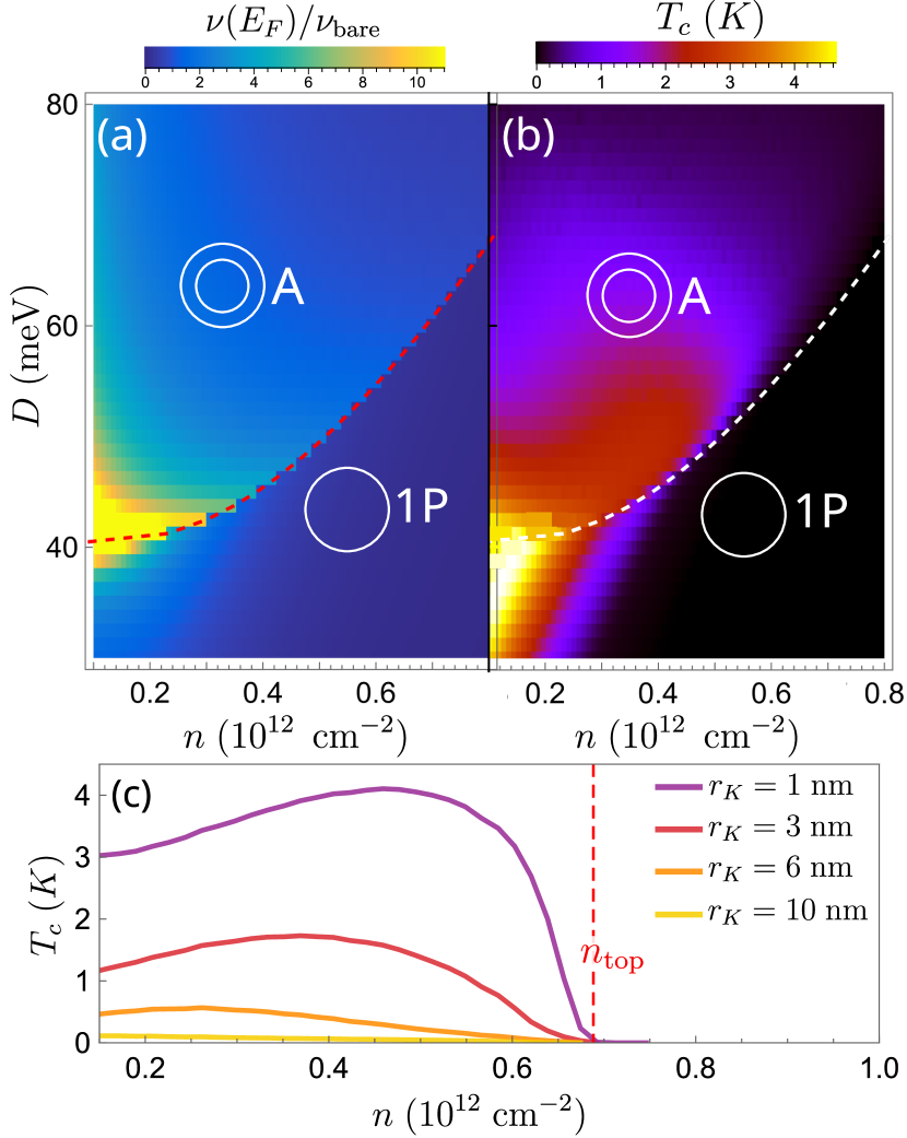
Figure 3: (a) Density of states of the minimal non-interacting model (Eq. (1)) normalized by $\nu_{e}=m_{e}/2\pi\hbar^{2}$ with $m_{e}$ the bare electron mass and (b) critical temperature of the chiral superconducting order as a function of electron density $n$ and displacement field $D$. The dashed line indicates the change in the Fermi sea from annular (A) to a single pocket (1P). We choose $r_{K}=3$ nm for the $T_{c}$ calculation. (c) Critical temperature for different dielectric screening parameterized by $r_{K}$.

Importantly, the screened interaction $\tilde{V}_{\bm{q}}$ is positive and large at momentum transfer $\bm{q}=\bm{k}-\bm{k}^{\prime}$ around $2k_{F,2}$, compared to small $\bm{q}$. Such $\bm{q}$-dependent interaction favors an order parameter that takes opposite signs at opposite $\pm\bm{k}$ points on the Fermi surface, i.e., it favors $p$-wave pairing.

For most superconductors, the pairing interaction is weak and therefore the pairing potential $\Delta(\bm{k})$ is small compared to the Fermi energy and only appreciable in the vicinity of the Fermi surface. For this reason, in solving the gap equation, it suffices to use “on-shell” pairing interaction $\tilde{V}_{l}(k,k^{\prime})$ at Fermi wavevectors $k,k^{\prime}$. In contrast, in multilayer graphene, the combination of low electron density and flat band bottom leads to a large ratio of interaction to the Fermi energy. As a consequence, we will show that $\Delta$ and $T_{c}$ can be on the order of the Fermi energy. Indeed, the recent experiment on tetralayer graphene [1] reports an unusually high upper critical field at at low density, indicating a strong-coupling superconductor with coherence length comparable to interparticle distance. For strong-coupling superconductors, the superconducting gap $\Delta(\bm{k})$ can be large even away from Fermi momentum. Therefore, in solving the gap equation it is necessary to use the interaction $\tilde{V}_{l}(k,k^{\prime})$ with full $k,k^{\prime}$ dependence.

Our calculation of $T_{c}$ as a function of electron density and displacement field is shown in Fig. 3(b)]. Both the displacement field $D$ and the electron density $n$ together determine the Fermi surface size and topology. For small $D<D_{c}\approx 40\,{\rm meV}$, the dispersion increases monotonously with $k$ and the Fermi surface is a single circle with $k_{F}=\sqrt{4\pi n}$, whereas at large displacement field ($D>D_{c}$), a Lifshitz transition from annular to simply-connected Fermi sea occurs with increasing electron density, which is accompanied by a large jump in the normal-state density of states at the Fermi level [Fig. 3(a)]. Correspondingly, superconducting properties depend strongly on the displacement field. For small $D$, a superconducting state is found at small density where the chemical potential lies close to the relatively flat band bottom with large density of states. For large $D$, the superconducting state sets in at low densities where the Fermi sea is annular, and $T_{c}$ is largest close to the Lifshitz transition.

It should be noted that the value of $T_{c}$ is sensitive to the dielectric screening of Coulomb repulsion by the multilayer graphene which, in turn, depends on the displacement field-induced band gap. As a function of the Rytova-Keldysh parameter $r_{K}$ [Fig. 3(c)], the typical $T_{c}$ at $D=60\,{\rm meV}$ ranges from $T_{c}\approx 3\,{\rm K}$ at $r_{K}=1\,{\rm nm}$ to a suppression of $T_{c}$ to below $0.1\,{\rm K}$ above $r_{K}=10\,{\rm nm}$. The decrease of $T_{c}$ with strong dielectric screening is consistent with electron pairing by Coulomb repulsion. Without knowing the value of $r_{K}$ for tetralayer graphene, we cannot make a quantitative prediction of $T_{c}$. Nonetheless, for the reasonable range of $r_{K}$ considered here, superconductivity always onsets at $n<0.7\times 10^{12}$ cm^-2 in agreement with experimental observation, and the calculated $T_{c}$ is acceptable compared to the experimental value, especially considering that the mean-field theory generally predicts higher values of $T_{c}$.

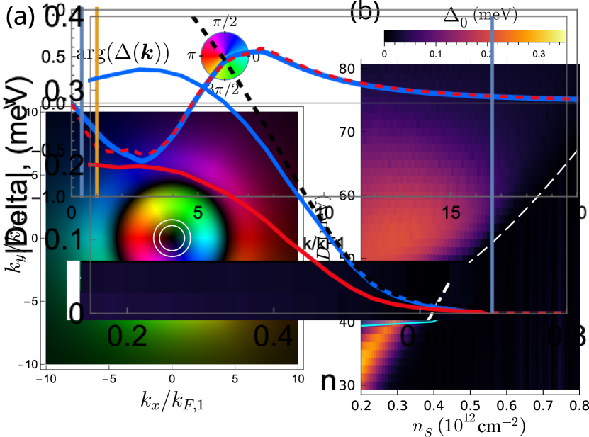
Figure 4: (a) Momentum-dependent $p$-wave pairing potential, where the tone (from black to light) indicates its magnitude and the hue corresponds to the complex phase. The white circles show the Fermi surfaces. (b) Zero-temperature spectral gap $\Delta_{0}=\min_{k}E_{k}$ as a function of displacement field and electron density $n_{S}$. The dashed white line indicates the change in the Fermi sea from annular (A) to a single pocket (1P). The cyan line bounds a (shaded) region at small densities and moderate displacement fields where $r_{s}\geq 40$.

Strong-coupling superconductivity.— For the chiral $p_{x}\pm ip_{y}$ pairing, the calculated pairing potential $\Delta(\bm{k})$ at $T=0$ can reach a few tenths of Fermi energy. Notably, $\Delta(\bm{k})$ is large not only close to the Fermi surface, but also extends to several times Fermi wavevector with a sign change at around $2k_{F,2}$ [Fig. 4(a)]. Its functional form closely follows the interaction potential up to a proportionality factor setting the pairing strength [see App. B]. The presence of substantial pairing potential away from the Fermi surfaces is a consequence of the strong-coupling nature of this superconducting state – because $k_{B}T_{c}$ and $\Delta$ are of order of the Fermi energy, pairing between electrons away from the Fermi surface is relevant. This is captured by our direct solution of Eqs. (10) and (11).

Due to the large pairing potential, the chemical potential changes appreciably in the superconducting state. This can be estimated by taking into account pairing potential in relating electron density to chemical potential

$$n_{s}=\int\frac{d{\bm{k}}}{4\pi^{2}}\left(1-\frac{\varepsilon_{k}-\mu}{E_{k}}\right).$$ (12)

At zero temperature, the change in chemical potential approaches $0.1\,{\rm meV}$. The change in electron density is taken into account in Fig. 4(b). Near $T_{c}$, the pairing potential is strongly temperature dependent $\Delta\propto\sqrt{1-T/T_{c}}$, and therefore the change in chemical potential $\delta\mu\propto|\Delta|^{2}$ is expected to increase linearly with decreasing temperature.

Topological superconductivity and Lifshitz transition.— The quasiparticle gap $\Delta_{0}\equiv\min_{k}E_{k}$ as a function of density $n$ and displacement field $D$ is shown in Fig. 4(c). Our $p\pm ip$ superconductor generally has a full gap, except at the Lifshitz transition from simply-connected to annular Fermi sea, where the system has a point node at the Fermi point $k=0$ at which the pairing potential vanishes. The closing of the quasiparticle gap marks a topological quantum phase transition from a topological superconductor with unity Chern number in the region with single Fermi pocket to a topologically trivial state in the annular region at large displacement fields [48, 49]. The topological superconductor at small displacement fields hosts chiral Majorana edge modes and Majorana zero modes in the vortex [3]. In contrast, the trivial state with annular Fermi sea is adiabatically connected to the Bose-Einstein limit $\mu\to-\infty$, because the pairing potential $\Delta(\bm{k})$ is finite at the band bottom of the Mexican hat dispersion which forms a ring at $k\neq 0$. Note that in our theory, even though the superconducting gap vanishes at $k=0$ at the Lifshitz transition, the gap at outer Fermi surface $\Delta(k_{F2})$ and critical temperature remains large throughout the transition– therefore the quasiparticle gap closure is not visible in the critical temperature calculations Fig. 3(b).

Competing state.— Since the $p$-wave superconductivity found in our RPA calculation occurs at relatively low density, it is important to consider its competition with the Wigner crystal state, which generally appears in 2D Coulomb systems at sufficiently low density. To estimate the transition to Wigner crystal, we compute the gas parameter $r_{s}=E_{\rm int}/E_{\rm kin}$ given by the ratio of interaction $E_{\rm int}$ to kinetic energy $E_{\rm int}$ [50]. In our calculations of $r_{s}$ here, we included a realistic distance $d=30\,{\rm nm}$ to the metallic gates, whose screening modifies the bare interaction potential $V_{q}\to V_{q}\tanh qd$. We verified that this this screening does not visibly affect our calculations of $T_{c}$ and superconducting gap; however $r_{s}$ depends sensitively on the gate screening as the interparticle distances at low density approaches tens of nm.

In Fig. 4, the region where $r_{s}>40$ is encircled by the cyan line; in a homogeneous electron gas the transition to a Wigner crystal occurs around $r_{s}\approx 30-40$ [51, 52, 50, 53, 54]. This region is where the band bottom is most flat, so that the kinetic energy per particle is low. It coincides with region where density of states is largest, see Fig. 3(a). We expect crystalline order is likely to dominate there, so that the superconducting region is divided in two, separated by the charge-ordered phase.

Trigonal warping and Berry curvature effects.— Our minimal model neglects trigonal warping, which arises from electron hoppings beyond nearest neighbor atoms in multilayer graphene. With trigonal warping, the band dispersion becomes asymmetric $\epsilon_{\bm{k}}\neq\epsilon_{-\bm{k}}$, which weakens intravalley pairing between $\pm k$ states. Fortunately, the energy scale of trigonal warping is small in tetralayer graphene in the range of density and displacement field of interest, as evidenced by the nearly symmetric band dispersion shown in Fig. 1. Furthermore, our superconducting state driven by Coulomb interaction has a large gap up to a few tenths of Fermi energy, and therefore is robust against the pair breaking effect of trigonal warping.

Up to now we have neglected the effect of electron Bloch wavefunctions $\ket{u_{\bm{k}}}$ within the unit cell. The momentum dependence of complex-valued wavefunction $\ket{u_{\bm{k}}}$ gives rise to Berry curvature breaking time reversal symmetry, when the system is valley polarized. We now show that the Berry-phase effect generally favors a particular chirality for $p$-wave pairing within a given valley. To see this, we note that the full interaction term for the electrons in the conduction band is generally of the form

$$\tilde{H}_{int}=\frac{1}{2}\sum_{\bm{k},\bm{k}^{\prime},\bm{q}}V(\bm{q})\bra{u_{-\bm{k}^{\prime}}}\ket{u_{-\bm{k}}}\bra{u_{\bm{k}^{\prime}}}\ket{u_{\bm{k}}}\widetilde{\psi}^{\dagger}_{\bm{k}+\bm{q}}\widetilde{\psi}^{\dagger}_{\bm{k}^{\prime}-\bm{q}}\widetilde{\psi}_{\bm{k}^{\prime}}\widetilde{\psi}_{\bm{k}}$$ (13)

where $\widetilde{\psi}^{(\dagger)}_{\bm{k}}$ creates an electron in the state $\ket{u_{\bm{k}}}$ in the conduction band. Compared to Eq. (2), the full interaction contains the form factor $\bra{u_{-\bm{k}^{\prime}}}\ket{u_{-\bm{k}}}\bra{u_{\bm{k}^{\prime}}}\ket{u_{\bm{k}}}$, which is complex-valued and thus breaks the time-reversal symmetry of low-energy theory.

We expand the form factor into harmonics

$$\bra{u_{-\bm{k}^{\prime}}}\ket{u_{-\bm{k}}}\bra{u_{\bm{k}^{\prime}}}\ket{u_{\bm{k}}}=\sum_{l}\alpha_{l}^{\tau}e^{-il(\varphi_{\bm{k}^{\prime}}-\varphi_{\bm{k}})}$$ (14)

where $\alpha_{l}^{\tau}=(\alpha_{-l}^{-\tau})^{*}$ due to time-reversal symmetry relating the two valleys $\tau=\pm 1$. The limit $\alpha_{l}\to 0$ for all $l\neq 0$ recovers our previous analysis using Eq. (2). Now, we treat $\alpha_{l}$ with $l\neq 0$ as a perturbation to the $p$-wave superconducting state.

Including the form factor, the condensation energy

$$E_{{\rm c}}=-\frac{1}{2A}\sum_{\bm{k},\bm{k}^{\prime}}\tilde{V}_{\bm{k}-\bm{k}^{\prime}}\bra{u_{-\bm{k}^{\prime}}}\ket{u_{-\bm{k}}}\bra{u_{\bm{k}^{\prime}}}\ket{u_{\bm{k}}}\langle\hat{\psi}_{-\bm{k}}\hat{\psi}_{\bm{k}}\rangle\langle\hat{\psi}_{\bm{k}^{\prime}}^{\dagger}\hat{\psi}_{-\bm{k}^{\prime}}^{\dagger}\rangle$$ (15)

For a pairing potential $\Delta(\bm{k})=\eta_{j}(k)e^{ij\varphi_{\bm{k}}}$ with angular momentum $j$, using the angular decomposition of the form factor Eq. (14) and the pairing interaction Eq. (9), $E_{{\rm c}}$ can be expressed as

$$E_{{\rm c}}=-A\sum_{l}\alpha_{l}^{\tau}\int\frac{dkdk^{\prime}}{2(2\pi)^{3}}kk^{\prime}\tilde{V}_{-l-j}(k,k^{\prime})\frac{\eta_{j}(k)\eta_{j}(k^{\prime})}{4E_{\bm{k}}E_{\bm{k}^{\prime}}}.$$ (16)

When the form factor is a constant, only $\alpha_{0}$ term is present and $\tilde{V}_{j}=\tilde{V}_{-j}$ guarantees equal condensation energy for $\pm j$ pairings. However, with broken time reversal symmetry, $\alpha_{l\neq 0}$’s are generally nonzero and therefore the condensation energy is generally different for the two $p$-wave chiralities. In particular, a large contribution from the terms $j=-l$ proportional to $\tilde{V}_{0}(k,k^{\prime})$ because $\tilde{V}_{0}(k,k^{\prime})$ is positive definite.

Within the two-band model of Ref. [39] giving rise to dispersion Eq. (1), the wavefunction is of the form $|u(\bm{k})\rangle=(1,\lambda e^{4i\varphi_{\bm{k}}})$, so that $\alpha_{4}\propto\lambda$ is the leading order correction in Eq. (14). Thus, in Eq. (16) for the condensation energy, the corrections for $j=\pm 1$ pairing are proportional to the angular harmonics $\tilde{V}_{3}$ and $\tilde{V}_{5}$, respectively, which lifts the degeneracy between the two chiralities.

Discussion.— We have shown that a strong-coupling chiral $p$-wave superconducting may emerge from charge fluctuations due to Coulomb repulsion in a spin- and valley-polarized state in multilayer graphene. The superconducting transition occurs at low density over a range of displacement fields where the band bottom is flat on the scale of the Fermi energy. In this range, increasing displacing field induces a Lifshitz transition from simply-connected to annular Fermi sea occurs which also marks a phase transition from a topological to a trivial superconducting state. The chirality of the Bloch wave functions which is responsible for the Berry curvature selects the chirality of the $p$-wave superconducting order parameter.

Our obtained critical temperature and density range is in rough agreement with a recent experiment in tetralayer graphene [1]. In the experiment, quantum oscillations and anomalous Hall conductance measurements indicate the spin- and valley polarization. Superconductivity emerges in a region which does not show clear quantum oscillations, which indicates a large density of states (effective mass) in the relevant density range, consistent with our theoretical picture, see Fig. 3(a) and (b).

We also speculate that a charge ordered state may appear very close to the Lifshitz transition at low density, where the density of states and the ratio of interaction to kinetic energy are the largest. In this scenario, the ordered state divides the superconducting region into two domes. A similar feature has been observed in the experiment [1].

Finally, we note that the intravalley pairing implies a large Cooper pair momentum of $\pm 2\bm{K}$ which is commensurate with the lattice [55, 56, 57, 58, 59, 20, 60]. We also verified that our mechanism strongly favors $p$-wave pairing over higher angular momenta, see App. D.

Acknowledgements.  We thank Long Ju, Tonghang Han, Paco Guinea, Tommaso Cea, Erez Berg, Zhiyu Dong and Andrea Young for helpful discussions. This work was supported by a Simons Investigator Award from the Simons Foundation. M.G. acknowledges support from the German Research Foundation under the Walter Benjamin program (Grant Agreement No. 526129603). M.D. was supported in part by the Walter Burke Institute for Theoretical Physics at Caltech. L.F. was supported in part by the U.S. Army DEVCOM ARL Army Research Office through the MIT Institute for Soldier Nanotechnologies under Cooperative Agreement number W911NF-23-2-0121. The numerical calculations were performed using the Julia programming language [61].

Appendix A Fit parameters for the dispersion

We fit our simplified dispersion Eq. (1) to the dispersion of the realistic 8-band model from Refs. [19, 23]. The obtained fit parameters as a function of $D$ and a comparison to the 8-band model are shown in Fig. 5.

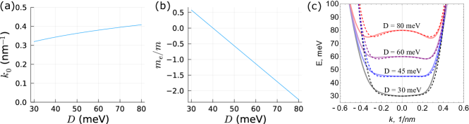
Figure 5: (a) Fit parameter $m$ and (b) $k_{0}$ of the Eq. (1). (c) Comparison of the minimal dispersion Eq. (1) with fitted parameters (dashed lines) to the 8-band model from Ref. [19, 23] (solid lines).

Appendix B Zero-temperature gap

A line plot of the radial profile of the zero-temperature superconducting gap is shown in Fig. 6(a). Interestingly, the radial profile of the superconducting gap follows closely the functional form $V_{l=1}(k_{F,2},k)$ of the first harmonic of the scattering potential when one of the scattering partners has momentum $k_{F,2}$ at the outer Fermi surface. Additionally, the radial profile of the superconducting gap at $T_{c}$ is very similar to the functional form at zero temperature (data not shown).

Fig. 6(b) shows the pairing potential at the inner and outer Fermi surface, as well as its maximum as a function of density, at the same parameters as the critical temperature data in Fig. 3(c) at $r_{K}=3\,{\rm nm}$. The ratio $\eta_{1}(k_{F,2}/k_{B}T_{c}$ slightly depends on density but remains close to two. The Bogoliubov quasiparticle dispersion at zero temperature and density $n=0.5\,10^{12}\,{\rm cm}^{-2}$ is shown in Fig. 6(c).

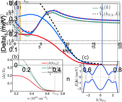
Figure 6: (a) Pairing potential $\eta_{1}(k)$ as a function of radial momentum $k$ and first harmonic of the interaction $\tilde{V}_{1}(k_{F,2},k)$ for density $n=0.5\,10^{12}\,{\rm cm}^{-2}$. (b) Pairing potential at the inner ($k_{F,1}$) and outer ($k_{F,2}$) Fermi surface and maximal magnitude $\max_{k}|\eta_{1}(k)|$. (c) Zero-temperature dispersion of Bogoliubov quasiparticles at $n=0.5\,10^{12}\,{\rm cm}^{-2}$. Here we use the displacement field $D=60\,{\rm meV}$ and Keldysh parameter $r_{K}=3\,{\rm nm}$.

Appendix C Gas parameter $r_{s}$

Fig. 7 (a) shows the gas parameter $r_{s}$ as a function of density and displacement field for a distance of $d=30\,{\rm nm}$ to the gates. Only when the dispersion is flat, the gas parameter reaches large values above 30, where a transition to a charge-ordered state typically occurs. The gas parameter is significantly suppressed by screening from the gates – when the gates are taken infinitely far away, the gas parameter is much larger, compare to Fig. 7 (b). This suggests that screening from the metallic gates plays an important role in suppressing a competing charge-ordered state.

(a) $d=30\,{\rm nm}$	(b) $d\to\infty$

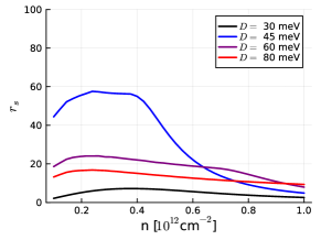
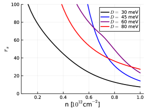
Figure 7: Gas parameter $r_{s}$ for distance to the metallic gates of (a) $d=30\,{\rm nm}$ and (b) $d\to\infty$.

Appendix D Higher angular momentum pairing

We investigate the higher angular momentum channels from our mechanism. Fig. 8 shows the zero temperature pairing potentials at the outer Fermi surface $k_{F,2}$ for $l=1,3$, and $5$, corresponding to $p$-, $f$-, and $h$-wave pairing. The pairing potetials are of the order of $10^{-3}\,{\rm meV}$, about two order of magnitude smaller than the typical pairing potential of $p$-wave pairing. A similar result hold for the critical temperature, where we found maximal $T_{c}$ of the order of $20{\rm mK}$, where the pairing state satisfies $k_{B}T_{c}/\Delta(k_{F,2}\approx 2$. In principle, $f$-wave and $h$-wave pairing are present at large density where $p$-wave is absent, however the corresponding critical temperatures and superconducting gaps are so small that these states are likely not observable.

(a) $D=30\,{\rm meV}$	(b) $D=60\,{\rm meV}$

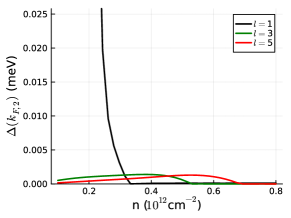
Figure 8: Zero-temperature pairing potentials for $p$-wave (l = 1), $f$-wave (l = 3), and $h$-wave (l = 5) for displacement fields (a) $D=30\,{\rm meV}$ and (b) $D=60\,{\rm meV}$.

Appendix E Mean-field theory

We perform the usual mean-field treatment and obtain the self-consistency equation:

$$\Delta(\bm{k})=\frac{1}{A}\sum_{\bm{k}^{\prime}}V(\bm{k}-\bm{k}^{\prime})\langle\psi_{-\bm{k}^{\prime}}\psi_{\bm{k}^{\prime}}\rangle$$ (17)

where for a ${\rm SO}(2)$ rotation-symmetric dispersion

$$\langle\hat{\psi}_{-\bm{k}}\hat{\psi}_{\bm{k}}\rangle=-\frac{\Delta(\bm{k})}{2E_{\bm{k}}}\tanh\frac{E_{\bm{k}}}{2k_{B}T}$$ (18)

where $E_{\bm{k}}=\sqrt{(\varepsilon(\bm{k})-\mu)^{2}+|\Delta_{\bm{k}}|^{2}}$.

Due to the ${\rm SO}(2)$ rotation symmetry, the pairing potential can be expanded in angular harmonics

$$\Delta(\bm{k})=\sum_{m=0}^{\infty}\eta_{m}(k)e^{im\theta}$$ (19)

where the equations for the critical temperature $T_{c}$ for different angular harmonics decouple, as we show below.

E.0.1 Linearized gap equation for solutions around $T_{\rm c}$

We describe a numerical procedure to obtain $T_{{\rm c},m}$ and the radial profile of the pairing potential $\eta_{m}(k)$ for different angular harmonics $m$.

Searching for solutions around the critical temperature $T_{\rm c}$, we may linearize in $\Delta({\bm{k}})$ so that $E_{\bm{k}}\approx|\xi_{\bm{k}}-\mu|$ and

$$\Delta(\bm{k})=-\frac{1}{A}\sum_{\bm{k}^{\prime}}\tilde{V}_{\bm{k}-\bm{k}^{\prime}}\frac{\Delta(\bm{k}^{\prime})}{2|\xi_{k^{\prime}}-\mu|}\tanh\frac{|\xi_{k^{\prime}}-\mu|}{2k_{B}T}$$ (20)

Expanding the pairing potential into angular harmonics, Fourier transformation reveals that different angular harmonics decouple, and we obtain Eq. (10) from the main text.

Eq. (10) equation can be solved iteratively as follows. Starting from an initial guess $\eta_{m}^{(0)}(k)$ (and for any iteration $\eta_{m}^{(n)}(k)$) for which we require only normalization $\int_{0}^{\infty}\eta_{m}^{(n)}(k)dk=1$, we obtain a corresponding $T_{{\rm c},m}^{(n)}$ by integrating over $\int_{0}^{\infty}dk_{1}$ to obtain a closed form expression,

$$1=-\frac{1}{2(2\pi)^{2}}\int_{0}^{\infty}dk\int_{0}^{\infty}dk^{\prime}k^{\prime}\tilde{V}_{m}(k,k^{\prime})\eta_{m}^{(n)}(k^{\prime})\frac{\tanh\frac{|\xi_{k^{\prime}}|}{2k_{B}T_{{\rm c},m}^{(n)}}}{|\xi_{k^{\prime}}-\mu|}$$ (21)

where for the second line we used the symmetry $\tilde{V}_{m}$. Having found $T_{{\rm c},m}^{(n)}$, we obtain the next iteration

$$\eta_{m}^{(n+1)}(k)=-\frac{1}{2(2\pi)^{2}}\int_{0}^{\infty}dk^{\prime}\tilde{V}_{m}(k,k^{\prime})\frac{\tanh\frac{|\xi_{k^{\prime}}|}{2k_{B}T_{{\rm c},m}^{(n)}}}{|\xi_{k^{\prime}}-\mu|}\eta_{m}^{(n)}(k^{\prime})$$ (22)

for which $T_{{\rm c},m}^{(n+1)}$ can then again be found using the above implicit equation. We found that the functional form of $\eta_{m}(k)$ is approximated by $\tilde{V}_{m}(k_{F,2},k)$ up to a factor setting the overall magnitude [compare to Fig. 6(a)], so that $\eta_{m}^{(0)}(k)=\tilde{V}_{m}(k_{F,2},k)$ is a good initial guess.

E.0.2 Zero-temperature gap

At zero temperature, the self-consistency equation simplifies

$$\Delta(\bm{k})=-\frac{1}{2A}\sum_{\bm{k}^{\prime}}V_{\bm{k}-\bm{k}^{\prime}}\frac{\Delta(\bm{k}^{\prime})}{E_{\bm{k}^{\prime}}}$$ (23)

Formally, this equation does not separate into individual angular harmonics $\eta_{m}(k)$ of the scattering potential. However, we anticipate that decoupled solutions solve the self-consistency equation and solve for the zero-temperature pairing potential of each angular momentum separately. This directly leads to Eq. (11) in the main text.

Eq. (11) equation can again be solved iteratively. With the Ansatz $\eta_{m}^{(0)}(k)=|\eta_{m}^{(0)}|f_{m}^{(0)}(k)$ in terms of magnitude $|\eta_{m}^{(0)}|$ and functional form $f_{m}^{(0)}(k)$ for which we require normalization $\int_{0}^{\infty}f_{m}^{(0)}(k)dk=1$, the magnitude is found self consistently by integration over $k$,

$$1=-\frac{1}{2(2\pi)^{2}}\int dk\int_{0}^{\infty}dk^{\prime}k^{\prime}V_{m}(k,k^{\prime})\frac{f_{m}^{(0)}(k^{\prime})}{||f_{m}^{(0)}||}\frac{1}{\sqrt{(\xi_{k^{\prime}}-\mu)^{2}+\left(|\eta_{m}^{(0)}|f_{m}^{(0)}(k^{\prime})\right)^{2}}}\,.$$ (24)

The functional form of the next iteration is then defined as

$$f_{m}^{(n+1)}(k)=-{\cal N}_{m}^{(n+1)}\frac{1}{2(2\pi)^{2}}\int_{0}^{\infty}dk^{\prime}k^{\prime}V_{m}(k,k^{\prime})\frac{f_{m}^{(n)}(k^{\prime})}{\sqrt{(\xi_{k^{\prime}}-\mu)^{2}+\eta_{m}^{(n)}(k^{\prime})^{2}}}$$ (25)

up to normalization, for which one then again determines the magnitude $|\eta_{m}^{(n)}|$ as above. A good ansatz for the starting point $f_{m}^{(0)}$ is the functional form $\eta_{m}(k)$ obtained at the critical temperature, or in terms of $\tilde{V}_{m}(k_{F,2},k)$ [see above and Fig. 6(a)].

References

- Han et al. [2024] T. Han, Z. Lu, Y. Yao, L. Shi, J. Yang, J. Seo, S. Ye, Z. Wu, M. Zhou, H. Liu, G. Shi, Z. Hua, K. Watanabe, T. Taniguchi, P. Xiong, L. Fu, and L. Ju, arXiv 10.48550/arXiv.2408.15233 (2024), 2408.15233 .
- Kallin and Berlinsky [2016] C. Kallin and J. Berlinsky, Rep. Prog. Phys. 79, 054502 (2016).
- Read and Green [2000] N. Read and D. Green, Phys. Rev. B 61, 10267 (2000).
- Sato and Ando [2017] M. Sato and Y. Ando, Rep. Prog. Phys. 80, 076501 (2017).
- Maeno et al. [1994] Y. Maeno, H. Hashimoto, K. Yoshida, S. Nishizaki, T. Fujita, J. G. Bednorz, and F. Lichtenberg, Nature 372, 532 (1994).
- Aoki et al. [2019] D. Aoki, A. Nakamura, F. Honda, D. Li, Y. Homma, Y. Shimizu, Y. J. Sato, G. Knebel, J.-P. Brison, A. Pourret, D. Braithwaite, G. Lapertot, Q. Niu, M. Vališka, H. Harima, and J. Flouquet, J. Phys. Soc. Jpn. 88, 043702 (2019).
- Jiao et al. [2020] L. Jiao, S. Howard, S. Ran, Z. Wang, J. O. Rodriguez, M. Sigrist, Z. Wang, N. P. Butch, and V. Madhavan, Nature 579, 523 (2020).
- Aoki et al. [2022] D. Aoki, J.-P. Brison, J. Flouquet, K. Ishida, G. Knebel, Y. Tokunaga, and Y. Yanase, J. Phys.: Condens. Matter 34, 243002 (2022).
- Kallin and Berlinsky [2009] C. Kallin and A. J. Berlinsky, J. Phys.: Condens. Matter 21, 164210 (2009).
- Mackenzie et al. [2017] A. P. Mackenzie, T. Scaffidi, C. W. Hicks, and Y. Maeno, npj Quantum Mater. 2, 1 (2017).
- Rømer et al. [2019] A. T. Rømer, D. D. Scherer, I. M. Eremin, P. J. Hirschfeld, and B. M. Andersen, Phys. Rev. Lett. 123, 247001 (2019).
- Kivelson et al. [2020] S. A. Kivelson, A. C. Yuan, B. Ramshaw, and R. Thomale, npj Quantum Mater. 5, 1 (2020).
- Røising et al. [2022] H. S. Røising, G. Wagner, M. Roig, A. T. Rømer, and B. M. Andersen, Phys. Rev. B 106, 174518 (2022).
- Ajeesh et al. [2023] M. O. Ajeesh, M. Bordelon, C. Girod, S. Mishra, F. Ronning, E. D. Bauer, B. Maiorov, J. D. Thompson, P. F. S. Rosa, and S. M. Thomas, Phys. Rev. X 13, 041019 (2023).
- Azari et al. [2023] N. Azari, M. Yakovlev, N. Rye, S. R. Dunsiger, S. Sundar, M. M. Bordelon, S. M. Thomas, J. D. Thompson, P. F. S. Rosa, and J. E. Sonier, Phys. Rev. Lett. 131, 226504 (2023).
- Andersen et al. [2024] B. M. Andersen, A. Kreisel, and P. J. Hirschfeld, Front. Phys. 12, 1353425 (2024).
- Zhou et al. [2021] H. Zhou, T. Xie, T. Taniguchi, K. Watanabe, and A. F. Young, Nature 598, 434 (2021).
- Chou et al. [2021] Y.-Z. Chou, F. Wu, J. D. Sau, and S. Das Sarma, Phys. Rev. Lett. 127, 187001 (2021).
- Ghazaryan et al. [2021] A. Ghazaryan, T. Holder, M. Serbyn, and E. Berg, Phys. Rev. Lett. 127, 247001 (2021).
- Li et al. [2021] T. Li, M. Geier, J. Ingham, and H. D. Scammell, 2D Mater. 9, 015031 (2021).
- You and Vishwanath [2022] Y.-Z. You and A. Vishwanath, Phys. Rev. B 105, 134524 (2022).
- Chatterjee et al. [2022] S. Chatterjee, T. Wang, E. Berg, and M. P. Zaletel, Nat. Commun. 13, 1 (2022).
- Ghazaryan et al. [2023] A. Ghazaryan, T. Holder, E. Berg, and M. Serbyn, Phys. Rev. B 107, 104502 (2023).
- Jimeno-Pozo et al. [2023] A. Jimeno-Pozo, H. Sainz-Cruz, T. Cea, P. A. Pantaleón, and F. Guinea, Phys. Rev. B 107, L161106 (2023).
- Qin et al. [2023] W. Qin, C. Huang, T. Wolf, N. Wei, I. Blinov, and A. H. MacDonald, Phys. Rev. Lett. 130, 146001 (2023).
- Pantaleón et al. [2023] P. A. Pantaleón, A. Jimeno-Pozo, H. Sainz-Cruz, V. x.-T.-j. Phong, T. Cea, and F. Guinea, Nat. Rev. Phys. 5, 304 (2023).
- Li et al. [2023] Z. Li, X. Kuang, A. Jimeno-Pozo, H. Sainz-Cruz, Z. Zhan, S. Yuan, and F. Guinea, Phys. Rev. B 108, 045404 (2023).
- Dong et al. [2023a] Z. Dong, L. Levitov, and A. V. Chubukov, Phys. Rev. B 108, 134503 (2023a).
- Dong et al. [2024] Z. Dong, É. Lantagne-Hurtubise, and J. Alicea, arXiv 10.48550/arXiv.2406.17036 (2024), 2406.17036 .
- Zhou et al. [2022] H. Zhou, L. Holleis, Y. Saito, L. Cohen, W. Huynh, C. L. Patterson, F. Yang, T. Taniguchi, K. Watanabe, and A. F. Young, Science 375, 774 (2022).
- Zhang et al. [2023] Y. Zhang, R. Polski, A. Thomson, É. Lantagne-Hurtubise, C. Lewandowski, H. Zhou, K. Watanabe, T. Taniguchi, J. Alicea, and S. Nadj-Perge, Nature 613, 268 (2023).
- Li et al. [2024] C. Li, F. Xu, B. Li, J. Li, G. Li, K. Watanabe, T. Taniguchi, B. Tong, J. Shen, L. Lu, J. Jia, F. Wu, X. Liu, and T. Li, Nature 631, 300 (2024).
- Cea et al. [2022] T. Cea, P. A. Pantaleón, V. x.-T.-j. Phong, and F. Guinea, Phys. Rev. B 105, 075432 (2022).
- Chou et al. [2022] Y.-Z. Chou, F. Wu, J. D. Sau, and S. Das Sarma, Phys. Rev. B 105, L100503 (2022).
- Dong et al. [2023b] Z. Dong, A. V. Chubukov, and L. Levitov, Phys. Rev. B 107, 174512 (2023b).
- Note [1] For a mean field study of superconductivity from attraction, see Ref. [62]).
- Sigrist and Ueda [1991] M. Sigrist and K. Ueda, Rev. Mod. Phys. 63, 239 (1991).
- Note [2] We verified that qualitatively similar results for the superconducting order are obtained when the functional form of the dispersion is varied, as long as the main qualitative features are preserved.
- Slizovskiy et al. [2019] S. Slizovskiy, E. McCann, M. Koshino, and V. I. Fal’ko, Commun. Phys. 2, 1 (2019).
- Rytova [2020] N. S. Rytova, Screened potential of a point charge in a thin film (2020), arXiv:1806.00976 [cond-mat.mes-hall] .
- Keldysh [1979] L. V. Keldysh, Soviet Journal of Experimental and Theoretical Physics Letters 29, 658 (1979).
- Cudazzo et al. [2011] P. Cudazzo, I. V. Tokatly, and A. Rubio, Phys. Rev. B 84, 085406 (2011).
- Quintela et al. [2022] M. F. C. M. Quintela, J. C. G. Henriques, L. G. M. Tenório, and N. M. R. Peres, Phys. Status Solidi B 259, 2200097 (2022).
- Kohn and Luttinger [1965] W. Kohn and J. M. Luttinger, Phys. Rev. Lett. 15, 524 (1965).
- Chubukov [1993] A. V. Chubukov, Phys. Rev. B 48, 1097 (1993).
- Maiti and Chubukov [2013] S. Maiti and A. V. Chubukov, AIP Conf. Proc. 1550, 3 (2013).
- Note [3] This angular decomposition applies for a circularly symmetric interaction potential, where the circular symmetry is preserved for the screened potential when the dispersion is circularly symmetric.
- Geier et al. [2020] M. Geier, P. W. Brouwer, and L. Trifunovic, Phys. Rev. B 101, 245128 (2020).
- Kitaev [2001] A. Y. Kitaev, Phys.-Usp. 44, 131 (2001).
- Drummond and Needs [2009] N. D. Drummond and R. J. Needs, Phys. Rev. Lett. 102, 126402 (2009).
- Tanatar and Ceperley [1989] B. Tanatar and D. M. Ceperley, Phys. Rev. B 39, 5005 (1989).
- Rapisarda and Senatore [1996] F. Rapisarda and G. Senatore, Aust. J. Phys. 49, 161 (1996).
- Spivak and Kivelson [2004] B. Spivak and S. A. Kivelson, Phys. Rev. B 70, 155114 (2004).
- Monarkha and Syvokon [2012] Yu. P. Monarkha and V. E. Syvokon, Low Temp. Phys. 38, 1067 (2012).
- Fulde and Ferrell [1964] P. Fulde and R. A. Ferrell, Phys. Rev. 135, A550 (1964).
- Larkin and Ovchinnikov [1964] A. I. Larkin and Y. N. Ovchinnikov, Zh. Eksperim. i Teor. Fiz Vol: 47 (1964).
- Roy and Herbut [2010] B. Roy and I. F. Herbut, Phys. Rev. B 82, 035429 (2010).
- Tsuchiya et al. [2016] S. Tsuchiya, J. Goryo, E. Arahata, and M. Sigrist, Phys. Rev. B 94, 104508 (2016).
- Li et al. [2020] T. Li, J. Ingham, and H. D. Scammell, Phys. Rev. Res. 2, 043155 (2020).
- Scammell et al. [2022] H. D. Scammell, J. Ingham, M. Geier, and T. Li, Phys. Rev. B 105, 195149 (2022).
- Bezanson et al. [2017] J. Bezanson, A. Edelman, S. Karpinski, and V. B. Shah, SIAM Rev. (2017).
- Chou et al. [2024] Y.-Z. Chou, J. Zhu, and S. D. Sarma, arXiv 10.48550/arXiv.2409.06701 (2024), 2409.06701 .