A Personalised 3D+t Mesh Generative Model for Unveiling Normal Heart Dynamics

Abstract

Understanding the structure and motion of the heart is crucial for diagnosing and managing cardiovascular diseases, the leading cause of global death. There is wide variation in cardiac shape and motion patterns, that are influenced by demographic, anthropometric and disease factors. Unravelling the normal patterns of shape and motion, as well as understanding how each individual deviates from the norm, would facilitate accurate diagnosis and personalised treatment strategies. To this end, we developed a novel conditional generative model, MeshHeart, to learn the distribution of cardiac shape and motion patterns. MeshHeart is capable of generating 3D+t cardiac mesh sequences, taking into account clinical factors such as age, sex, weight and height. To model the high-dimensional and complex spatio-temporal mesh data, MeshHeart employs a geometric encoder to represent cardiac meshes in a latent space, followed by a temporal Transformer to model the motion dynamics of latent representations. Based on MeshHeart, we investigate the latent space of 3D+t cardiac mesh sequences and propose a novel distance metric termed latent delta, which quantifies the deviation of a real heart from its personalised normative pattern in the latent space. In experiments using a large dataset of 38,309 subjects, MeshHeart demonstrates a high performance in cardiac mesh sequence reconstruction and generation. Features defined in the latent space are highly discriminative for cardiac disease classification, whereas the latent delta exhibits strong correlation with clinical phenotypes in phenome-wide association studies. The codes and models of this study will be released to benefit further research on digital heart modelling.

Introduction

The heart is one of the most important and vital organs within the human body [1]. It is composed of four morphologically distinct chambers that function in a coordinated manner. The shape of the heart is governed by genetic [2] and environmental factors, as well as a remodelling process observed in response to myocardial infarction, pressure overload, and cardiac diseases [2, 3]. The motion of the heart follows a periodic non-linear pattern modulated by the underlying molecular, electrophysiological, and biophysical processes [4]. The unveiling of complex patterns of cardiac shape and motion will provide important information to assess the status and function of the heart for both clinical diagnosis and cardiovascular research [5, 6, 7, 8].

The current state-of-the-art for assessing cardiac shape and function is to perform analyses of cardiac images, e.g., cardiac magnetic resonance (MR) images, and extract imaging-derived phenotypes (IDPs) of cardiac chambers [bai2020population，Dewey2020]. Most imaging phenotypes, such as chamber volumes or ejection fractions, provide a global and simplistic measure of the complex 3D-temporal (3D+t) geometry of cardiac chambers [9]. These measures may not fully capture the dynamics and variations of heart function across individuals. Recognising these limitations underscores the importance of establishing a more precise model of cardiac status, defining what a normal heart looks like and moves like. Nevertheless, it is a non-trivial task to describe the normative pattern of the 3D shape or even 3D-t motion of heart, due to the complexity in representing high-dimensional spatio-temporal data.

Recently, machine learning techniques have received increasing attention for cardiac shape and motion analysis [4, 10, 11]. Most existing research focuses on developing discriminative machine learning models, that is, training a model to perform classification tasks between different shapes or motion patterns [12, 13, 4, 6]. However, discriminative models offer only classification results and do not explicitly explain what the normative pattern of cardiac shape or motion looks like [14]. In contrast, generative machine learning models provide an alternative route. Generative models are capable of describing distributions of high-dimensional data, such as images [15, 16, 17], geometric shapes [18, 19, 20], or molecules [21, 22], which allow the representation of normative data patterns in the latent space of the model. Although generative models have been explored for cardiac shape modelling [23, 24, 25, 26, 27] or for cardiac imaging data augmentation [28], their application to personalised normative modelling of the heart has been less explored.

Here, we provide the first endeavour to create a personalised normative model of 3D+t cardiac shape and motion, leveraging deep generative modelling techniques. Cardiac shape and motion are represented by a dynamic sequence of 3D surface meshes across a cardiac cycle. A novel geometric deep generative model, named MeshHeart, is developed to model the distribution of 3D+t cardiac mesh sequences. MeshHeart employs a graph convolutional network (GCN) [29] to learn the latent features of the mesh geometry and a Transformer to learn the temporal dynamics of the latent features during cardiac motion. This integration enables MeshHeart to model the distributions across both spatial and temporal dimensions. MeshHeart functions as a conditional generative model, accounting for major clinical variables such as sex and age as the generation factor. This enables the model to describe personalised normative patterns, generating synthetic healthy cardiac mesh sequences for a specific patient or a specific subpopulation.

We train the proposed generative model, MeshHeart (Figure 1(a)), on a large-scale population-level imaging dataset with 38,309 subjects from the UK Biobank [7, 30]. After training the model, for each individual heart, we can generate a personalised 3D+t cardiac mesh model that describes the normative pattern for this particular subpopulation that has the same clinical factors as the input heart, as illustrated in Figure 1(c). In qualitative and quantitative experiments, we demonstrate that MeshHeart achieves high accuracy in generating the personalised heart model. Furthermore, we investigates the clinical relevance of the latent vector $z$ of the model and propose a novel distance metric (latent delta $\Delta z$), which measures the deviation of the input heart from its personalised normative pattern (Figure 1 (c)). We demonstrate that the latent vector and latent delta have a highly discriminative value for the disease classification task and they are associated with a range of clinical features in phenome-wide association studies.

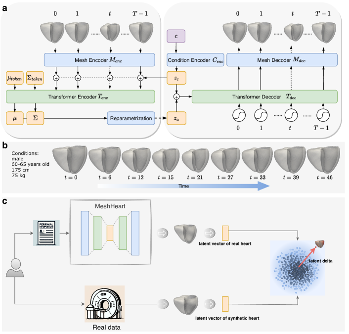
Figure 1: An overview of the MeshHeart model. a, Model architecture: MeshHeart encodes a sequence of cardiac meshes using a mesh encoder $M_{enc}$ and encodes clinical factors using a conditional encoder $C_{enc}$. The encoder outputs across the time frames and along with distribution tokens $\mu_{token}$ and $\Sigma_{token}$, are processed by a temporal Transformer encoder $T_{enc}$. A Transformer decoder $T_{dec}$ and a mesh decoder $M_{dec}$ generate a 3D cardiac mesh sequence based on clinical conditions. b, Given a set of clinical factors, an example of the generated mesh sequence across time frames. c, Conceptual framework: MeshHeart constructs a normative cardiac mesh sequence using personal information including age, sex, weight, and height. A real heart can be compared to its personalised norm by the latent vector. The latent delta $\Delta z$ is the computed distance between the latent vector of a synthetic normal heart (blue dot) and that of the real heart (red dot).

Results

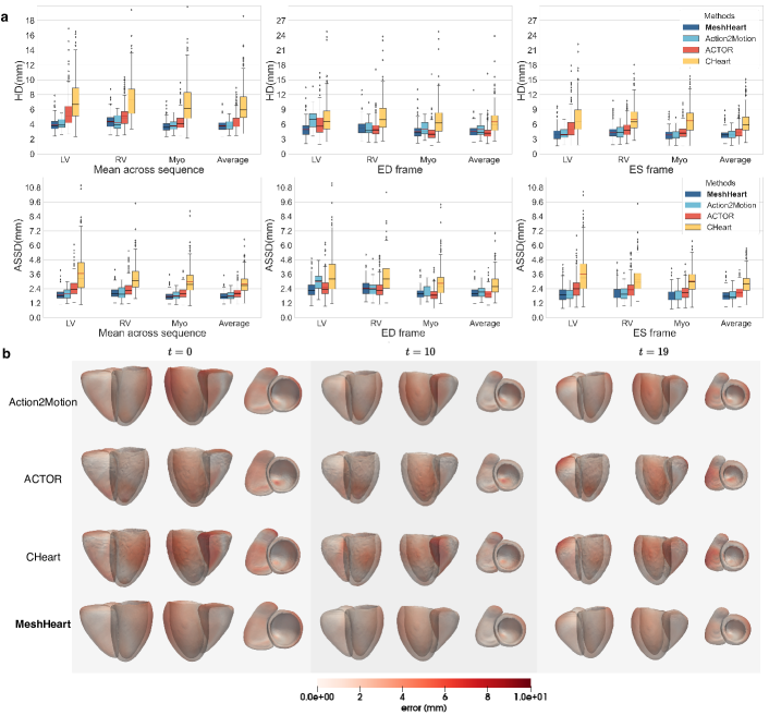
Figure 2: Evaluation of the mesh reconstruction accuracy of MeshHeart, compared to three other methods; Action2Motion, ACTOR, and CHeart. a, Plots of the Hausdorff distance (HD) and average symmetric surface distance (ASSD) metrics. The metrics are calculated as the mean across all time frames, as well as at the end-diastolic frame (ED) and the end-systolic frame (ES). They are reported for the left ventricle (LV), the myocardium (Myo), the right ventricle (RV), and averaged across the anatomical structures. Lower values indicate better performance. b, Visualisation of the reconstructed cardiac mesh sequence, coloured by the reconstruction error (in red) between the input mesh and reconstructed mesh. The mesh is visualised in three different imaging planes.

MeshHeart learns spatial-temporal characteristics of the mesh sequence

We first assessed the reconstruction capability of MeshHeart for 3D+t cardiac mesh sequences. The experiments used a dataset of 4,000 test subjects, with dataset detail described in Supplementary Table S1. Each input mesh sequence was encoded into latent representation and then decoded to reconstruct the mesh sequence. Reconstruction performance was evaluated using two metrics, the Hausdorff distance (HD) and the average symmetric surface distance (ASSD), which measure the difference between the input and reconstructed meshes. The HD metric quantifies the maximum distance between points in two sets, highlighting the maximum discrepancy between the original and reconstructed heart meshes. ASSD computes the average distance between the surfaces of two meshes, providing a more holistic evaluation of the model’s accuracy. Evaluation was performed for three anatomical structures: the left ventricle (LV), the myocardium (Myo), and the right ventricle (RV). We compared the performance of MeshHeart to three baseline mesh generative models: Action2Motion [20], ACTOR [31], and CHeart [26].

Figure 2(a) and Supplementary Table S2 report the reconstruction accuracy of MeshHeart, compared to other generative models. The metrics are reported as the average across all time frames, as well as at two representative time frames of cardiac motion: the end-diastolic frame (ED) and the end-systolic frame (ES). Overall, MeshHeart achieves the best reconstruction accuracy, outperforming other generative models, with the lowest HD of 4.163 mm and ASSD of 1.934 mm averaged across the time frames and across anatomical structures. Additionally, Figure 2(b) visualises examples of the reconstructed meshes, with vertex-wise reconstruction errors overlaid, at different frames of the cardiac cycle ($t=0,10,19$ out of 50 frames in total). MeshHeart achieves lower reconstruction errors compared to the other models and maintains the smoothness of reconstructed meshes. We further conducted ablation studies to assess the contribution of each component to the model performance. These components are described in the Methods section and the detailed results are reported in Supplementary Table S5. Replacing GCN by linear layers results in an increased HD from $4.163\leavevmode\nobreak\ mm$ to $5.707\leavevmode\nobreak\ mm$, while replacing GCN by CNN results in a HD of $5.268\leavevmode\nobreak\ mm$, highlighting GCN’s superiority in encoding mesh geometry. Substituting the Transformer with GRUs or LSTMs leads to an increased HD of $4.720\leavevmode\nobreak\ mm$ or $5.015\leavevmode\nobreak\ mm$, respectively, which demonstrates the advantage of using the Transformer for modelling long-range temporal dependencies. Other components such as the smoothness loss term and the distribution parameter tokens also contribute to the model performance. These results highlight MeshHeart’s capability in learning spatial-temporal characteristics of cardiac mesh sequences.

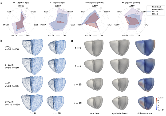
Figure 3: Evaluation of the generation performance of MeshHeart. a, Spider charts for the Wasserstein distance (WD) and the Kullback-Leibler(KL) divergence metrics, which quantify the distance between the generated and real data distributions. The data distribution is calculated as the histogram of a cardiac imaging phenotype (left ventricular end-diastolic volume (LVEDV), LV end-systolic volume (LVESV), LV ejection fraction (LVEF), LV myocardial mass (LVM), right ventricular end-diastolic volume (RVEDV), RV end-systolic volume (RVESV) and RV ejection fraction (RVEF)) against a clinical factor (age or sex). The metrics are plotted over a polar coordinate system, colour-coded by different methods. The smaller the metric (closer to the centre), the greater the similarity between the generated and real data distributions. b, Examples of generated 3D+t cardiac meshes with different generating factors, including age (a), sex (f/m for female/male), weight (w), and height (h). c, A side-by-side comparison of a real heart, the generated synthetic heart, and the difference map between them.

MeshHeart resembles real data distribution

Utilising the latent representations learnt by MeshHeart, we assessed the ability of the model to generate new synthetic cardiac mesh sequences that mimic real heart dynamics. To evaluate the fidelity and diversity of the generation, we calculated the similarity between the distributions of real meshes and generated synthetic meshes. For each real heart in the test set ($n=4,000$), we applied MeshHeart to generate synthetic mesh sequences using the same clinical factors (age, sex, weight, and height) as the individual as the model input. During the generation stage, we chose 20 random samples from the Gaussian distribution of the latent space and generated the corresponding mesh sequences. For both real and synthetic meshes, clinically relevant metrics for cardiac structure and function were derived, including left ventricular end-diastolic volume (LVEDV), LV end-systolic volume (LVESV), LV ejection fraction (LVEF), LV myocardial mass (LVM), right ventricular end-diastolic volume (RVEDV), RV end-systolic volume (RVESV) and RV ejection fraction (RVEF). For each metric $m$, its probability distributions against age $P(m|c=age)$ and against sex $P(m|c=gender)$, were calculated. The similarity between real and synthetic probability distributions was quantified using the Kullback-Leibler (KL) divergence [32] and the Wasserstein distance (WD) [33], with a lower value denoting a higher similarity, i.e. better generation performance. KL divergence is a metric from information theory that evaluates the dissimilarity between two probability mass functions. Similarly, WD measures the dissimilarity between two probability distributions. MeshHeart’s ability to replicate real data distributions is quantitatively demonstrated in Figure 3(a). MeshHeart achieves lower KL and WD scores compared to existing methods, as shown by radar plots with the smallest area, suggesting that the synthetic data generated by the proposed model closely aligns with the real data distribution for clinically relevant metrics. Supplementary Tables S3 and S4 report the detailed KL divergence and WD scores for different methods.

For qualitative assessment, Figure 3(b) presents four instances of synthetic cardiac mesh sequences for different personal factors (age, sex, weight, and height). For brevity, only two frames ($t=0,20$) are shown. The figure demonstrates that MeshHeart can mimic authentic cardiac movements, showing contractions across time from diastole to systole. Figure 3(c) compares a real heart with a synthetic normal heart, at different time frames ($t=0,5,15,19$), demonstrating the capability of MeshHeart in replicating both the real cardiac structure as well as typical motion patterns.

We also examined the latent representation learnt by MeshHeart using t-SNE (t-distributed Stochastic Neighbour Embedding) visualisation [34] as illustrated in Supplementary Figure S1. The t-SNE plot projects the 64-dimensional latent representation of a mesh, extracted from the last hidden layer of the Transformer Encoder $T_{enc}$, onto a two-dimensional space, with each point denoting a mesh. It shows 10 sample sequences. For each sample, the latent representations of the meshes across time frames form a circular pattern that resembles the rhythmic beating of the heart [35].

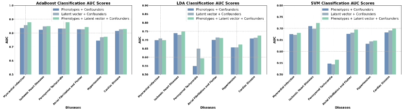
Figure 4: Comparison of disease classification performance, in terms of the AUC (area under the curve) scores, when different feature sets are used. The three feature sets being compared include "Phenotypes $+$ Confounders (Age, Sex)", "Latent vector $+$ Confounders", and "Phenotypes $+$ Latent vector $+$ Confounders", with each feature set represented by a unique color in the plot. The three subplots show the performance of three different classifiers, AdaBoost, LDA, and SVM. The x-axis denotes the disease type and the y-axis denotes the AUC score.

MeshHeart latent vector improves cardiovascular disease classification performance

After demonstrating the generative capability of MeshHeart, we explore its potential for clinical applications, in particular using its latent space which provides a low-dimensional representation of cardiac shape and motion. The latent feature analyses were conducted on 17,309 subjects. More than half (58.5%) had a reported diagnosis of at least one disease. We employ the latent vector $z$ of each mesh sequence, a 64-dimensional vector, as the feature for correlation analysis and for cardiac disease classification. Figure 5(a) shows that the latent vector exhibits strong correlations with conventional imaging phenotypes, such as LVM, LVEDV, and RVEDV etc. Figure 4 and Supplementary Table S6 compare the classification performance of six cardiac diseases when using different feature sets. The three evaluated feature sets include "Phenotypes + Confounders (Age, Sex)", "Latent Vector + Confounders", and "Phenotypes + Latent Vector + Confounders". The classification performance is evaluated using the AUC (area under the curve) scores for three different classifiers: AdaBoost, linear discriminant analysis (LDA), and support vector machine (SVM). The six cardiovascular diseases include myocardial infarction (ICD-10 code I21), ischemic heart diseases (I24), paroxysmal tachycardia (I47), atrial fibrillation and flutter (I48), hypertension (I10), and cardiac disease (I51). Figure 4 shows that using imaging phenotypes alone led to moderate AUC scores (e.g., 0.8361 and 0.8201 for myocardial infarction and ischemic heart diseases using with AdaBoost). Using the latent vector resulted in increased AUC scores (0.8557 and 0.8453). Combining both imaging phenotypes and the latent vector further improved the AUC scores (0.8762 and 0.8472), indicating the usefulness of the latent vector for cardiovascular disease classification.

For the AdaBoost classifier, using feature sets comprising the latent vector, as well as the combination of phenotypes and the latent vector, consistently outperformed the performance of the phenotypes set alone (e.g., 0.8291 and 0.8316 for cardiac disease using latent vector and combined feature sets), implying that incorporating the latent vector improved the classification accuracy. The trend was particularly noticeable for myocardial infarction, hypertension, and cardiac diseases, where the combined phenotypes and latent vector feature set substantially improved the AUC scores (0.8762, 0.7738 and 0.8316 for myocardial infarction, hypertension and cardiac disease). The LDA and SVM classifiers demonstrated that of the three feature sets, the combined phenotypes and latent vector feature set achieved the highest AUC scores (e.g., 0.6728 and 0.6479 for hypertension with LDA and SVM). However, for certain diseases such as ischemic heart disease, classifiers using only phenotypes (e.g., 0.7381 and 0.7123 for ischemic heart diseases with LDA and SVM) outperformed those that used only the latent vector (0.7277 and 0.6975), but still fell short of their combination (0.7492 and 0.7214). Overall, the results show that integrating imaging phenotypes, the latent vector along with confounders provides the best discriminative feature set for classification.

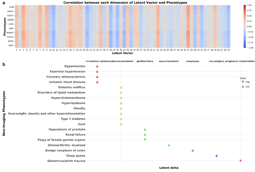
Figure 5: Association studies for the latent vector and the latent delta with imaging-derived phenotypes and clinical features. a, Heatmap of the Pearson correlation coefficients between imaging phenotypes and the 64-dimensional latent vector. The intensity of the colour reflects the magnitude and direction of the correlation, where blue signifies negative correlations and red signifies positive correlations. Darker shades indicate a stronger correlation between the vector and the phenotypes. b, Phenome-wide association study (PheWAS) between the latent delta $\Delta z$ and unbiased categories of clinical features. The y-axis lists the clinical outcomes where a signficiant association was identified. The x-axis uses different colors to represent different disease categories. Each triangle denotes a significant PheWAS association, adjusted for multiple comparisons using the Bonferroni correction for 1,163 clinical features analysed. These clinical features encompass both clinical outcomes (e.g., diseases and diagnoses) and phenotypes, covering a wide range of characteristics and measurements. The shape of each triangle indicates the direction of the effect. This analysis included 17,000 participants.

Latent delta for phenome-wide association studies (PheWAS)

For each individual heart, we use MeshHeart to generate a normal synthetic heart using the same clinical factors as this individual. This synthetic heart can be regarded as a personalised normative model learnt from a specific subpopulation. We define the latent delta $\Delta z$ to be the difference between the latent vectors of an individual heart and its personalised norm, quantified using the Euclidean distance. The latent delta characterises the deviation of the shape and motion patterns of an individual heart from the normal pattern for a subpopulation with the same clinical factors (Figure 1(c)). A phenome-wide association study (PheWAS) was performed to explore the clinical relevance of $\Delta z$, as shown in Figure 5(b). The PheWAS revealed significant associations between the latent delta $\Delta z$ and an unbiased set of clinical outcomes, including circulatory system diseases, endocrine/metabolic diseases, genitourinary diseases, musculoskeletal diseases and neoplasms.

The latent delta has been shown to correlate with phenotypes such as LVM and LVEF (Figure 5(a)), which serve as indicators of cardiac structure and function. Conditions such as hypertension, lipid/cholesterol abnormalities, and diabetes can induce changes in these cardiac phenotypes. For example, hypertension likely results in an increased LVM and may be linked to a reduced LVEF due to the heart’s adaptation to prolonged high blood pressure. In a similar vein, diabetes can exert metabolic stress on the heart, which can lead to changes in cardiac volume and ejection fraction. These modifications in the structure and motion patterns of the heart, as captured by the latent delta, provide a mechanistic explanation for the associations observed in the PheWAS results. Consequently, significant correlations between the latent delta and various clinical outcomes highlight its potential as a valuable marker for linking cardiac phenotypes with broader health conditions.

Discussion

This work contributes to the growing field of generative artificial intelligence for science, with a specific application in cardiac imaging. The proposed MeshHeart model is a new generative model that can facilitate improved understanding of the complexities of 3D+t cardiac shape and motion. In this study, we made four major contributions. First, we developed MeshHeart using a dataset of 38,309 subjects from a large UK population [30], capturing the variation in cardiac structures and clinical characteristics. Second, we demonstrated MeshHeart’s capability to generate a normal heart, accounting for clinical factors such as age, sex, weight, and height. This established a personalised normative model for cardiac anatomy. Third, we investigated the latent vector of MeshHeart and demonstrated its associations with conventional imaging phenotypes and usefulness for enhancing disease classification performance. Finally, we propose a novel latent delta ($\Delta z$) metric. This metric provides a way for quantifying the difference between an individual heart and the normative model, as well as for investigating the associations between the spatial-temporal characteristics of the heart and various health outcomes.

MeshHeart’s reconstruction capability was assessed using HD and ASSD metrics. Using these two metrics, we compared the model with other models along with an ablation study. Employing geometric convolutions and a temporal Transformer, the model reconstructed more accurate cardiac mesh sequences compared to the other state-of-the-art models. This is is due to the reason that geometric convolutions are proficient in encoding mesh geometry, and the Transformer is effective in capturing long-range temporal dependencies. The ablation study confirms the essential role of geometric convolutions and the temporal Transformer in increasing the performance of the model, as detailed in the Supplementary Table S5. We also compared MeshHeart against a previous work CHeart [26]. CHeart employs segmentation as a representation method for the cardiac structure, whereas MeshHeart employs the mesh representation. The results show that mesh provides a powerful representation for modelling the 3D geometry as well for tracking temporal motion, as it essentially allows monitoring the movement of each individual point over time.

The generative capabilities of MeshHeart, as illustrated by the results in Figure 3 and Supplementary Tables S3 and S4, demonstrate its proficiency as a generative model, able to replicate a ’normal’ heart based on certain clinical factors including demographics (age, sex) and anthropometrics (weight, height). These four factors have shown strong correlations with heart structure and function across various individuals [36, 37, 7]. They form a reliable basis for constructing a normal heart model for an individual, as shown in Figure 3(b). Our analysis in Figure 3(a) and Supplementary Tables S3 and S4 focused on age and sex, employing WD and KL divergence to assess the similarity between the real and synthetic data distributions. Lower WD and KL metrics suggest that MeshHeart effectively represents demographic diversity, making the synthetic data beneficial for potential clinical and research purposes. The incorporation of additional clinical variables in the future, such as blood pressure and medical history, could improve the representation of cardiac health and diseases, thus enabling more potential applications for downstream tasks.

The latent vector obtained from the MeshHeart demonstrated its discriminative power for disease classification tasks. Incorporating the latent vector as feature substantially improves the classification accuracy for a range of cardiovascular conditions, as illustrated in Figure 4. Although conventional imaging phenotypes can also be used as a feature set for the classification model, their classification performance was surpassed by the augmented feature set that also includes the latent vector, suggesting that the latent vector may contain some information not provided by the imaging phenotypes. Combining imaging phenotypes with the latent vector and confounders consistently achieved the best classification performance, regardless of the classification model used, demonstrating the benefit of integrating multiple data sources to represent the status of the heart. Some dimensions of the latent vector exhibit high correlations with conventional cardiac phenotypes, which are essential for assessing cardiovascular disease risk. The high correlation with the latent vector underscores their clinical analysis potential.

PheWAS uses a data-driven approach to uncover unbiased associations between cardiac deviations and disease diagnoses. Our analysis found that greater deviations in heart function are linked to increased risks of endocrine/metabolic and circulatory diseases. These cardiac diseases suggest underlying metabolic problems such as insulin resistance or metabolic disturbances observed in diabetes and obesity, which affect the structure and performance of the heart [38, 39]. Likewise, they indicate wider circulatory conditions such as hypertension and atherosclerosis, which can lead to heart failure and ischemic heart disease[40]. Understanding these relationships is crucial for risk stratification, personalised medicine, and prevention strategies, highlighting the need for thorough cardiac evaluations in clinical management [41].

Although this work advances the science in personalised cardiac modelling, there are several limitations. First, the personalised normative model relies on a restricted range of generating factors, including age, sex, weight, and height, as we aim to develop a standard healthy heart. Including additional elements in the future such as diseases or environmental factors such as air pollution and noise[42] could improve our understanding of their impacts on cardiac anatomy and function. Second, the model uses a cross-sectional dataset from the UK Biobank for both training and testing purposes. However, it does not include a benchmark for the progression of cardiac aging, which could be addressed by employing a longitudinal dataset to evaluate the model. Repeated scans are expected in the near future from the UK Biobank. Third, this study focuses on modelling the dynamic mesh sequence to describe cardiac shape and motion. It does not aim to model the underlying electrophysiology or biomechanics of the heart, which are also essential for cardiac modelling and understanding cardiac function [43, 44]. Additionally, the explainability of latent vectors could be explored, as understanding the specific information each latent dimension captures is crucial for clinical interpretation and validation.

In conclusion, this study presents MeshHeart, a generative model for cardiac shape modelling. By training and evaluating the model on a population-level dataset from the UK Biobank, we demonstrate that MeshHeart not only achieves a high reconstruction accuracy but also excels in generating synthetic cardiac mesh sequences that closely resemble the real heart. The latent vector of the generative model and the novel latent delta metric provide new avenues of research to improve disease classification and personalised healthcare. These findings pave the way for future research on cardiac modelling and may inspire the development of generative modelling techniques for other types of biomedical data.

Methods

Generative model

Figure 1(a) illustrates the architecture of the proposed generative model, MeshHeart. Given a set of clinical conditions $c$, our goal is to develop a model that can generate a dynamic 3D cardiac mesh sequence, $X_{0:T-1}=\{x,x_{1},\cdots,x_{T-1}\}$, where $T$ denotes the number of time frames, that corresponds to the conditions $c$. Figure 1(b) shows an example of the input conditions and the generated mesh sequence. Without losing generality, we take age, sex, weight and height as conditions $c$ in this work. Age, weight and height are continuous variables, whereas sex is a binary variable. Each cardiac mesh $x_{t}=(v_{t},e_{t})$ is a graph with a set of vertices $v$ and a set of edges $e$ connecting them. The proposed generative model consists of several components, a mesh encoder $M_{enc}$ and a condition encoder $C_{enc}$ to project the mesh sequence and conditions into latent representations, a Transformer encoder $T_{enc}$ to capture the temporal dependency of the meshes at different time frames, and finally a Transformer decoder $T_{dec}$ and a mesh decoder $M_{dec}$ to decode the latent representations back to the mesh sequence. The mesh encoder $M_{enc}$, constructed using a graph convolutional network (GCN), extracts features from the cardiac mesh sequence $x_{0:T-1}$ and generates latent vectors $z_{0:T-1}$. The condition encoder $C_{enc}$, implemented with a multi-layer perceptron (MLP), maps the clinical conditions $c$ into a condition latent vector $z_{c}$ in the condition latent space. The mesh latent vectors $z_{0:T-1}$ at each time frame are concatenated with the condition latent vector $z_{c}$, which forms a sequence of input tokens to the Transformer decoder $T_{dnc}$. For simplicity, the concatenated vectors are still denoted as $z_{0:T-1}$. These components work together to learn the probability distribution of the cardiac mesh sequence $x$ conditioned on $c$, assuming that the latent space follows a Gaussian distribution. We seek a model $p_{\theta}(x|z_{c})$, parameterised by $\theta$, that is sufficiently flexible to learn to describe the mesh sequence $x$.

We assume a prior distribution $p(z_{a})$ over the latent variable $z_{a}$. The prior $p(z_{a})$ together with the decoder (constructed by $T_{dec}$ and $M_{dec}$) $p(x,z_{a}|z_{c})$, define a joint distribution, denoted as $p(x|z_{c})$. To train the model and perform inference, we need to compute the posterior distribution $p(z_{a}|x,z_{c})$, which is generally intractable. To turn the intractable posterior inference problem $p(z_{a}|x,z_{c})$ into a tractable problem, we introduce a parametric encoder model (constructed by $C_{enc},M_{enc},T_{enc}$) $q_{\phi}(z_{a}|x,z_{c})$ with $\phi$ to be the variational parameters, which approximates the true but intractable posterior distribution $p(z_{a}|x,z_{c})$ of the generative model, given an input $x$ and conditions $c$:

$$q_{\phi}(z_{a}|x,z_{c})\approx p_{\theta}(z_{a}|x,z_{c})$$ (1)

where $q_{\phi}(z_{a}|x,z_{c})$ often adopts a simpler form, e.g. the Gaussian distribution. By introducing the approximate posterior $q_{\phi}(z_{a}|x,z_{c})$, the log-likelihood of the conditional distribution $p_{\theta}(x|z_{c})$ for input data $x$, also known as evidence, can be formulated as:

$$\log{p_{\theta}(x|z_{c})} =\mathbb{E}_{z_{a}\sim q_{\phi}(z_{a}|x,z_{c})}\log\left[{p_{\theta}(x|z_{c})}\right]$$ (2)

$$=\mathbb{E}_{z_{a}\sim q_{\phi}(z_{a}|x,z_{c})}\log\left[{\frac{p_{\theta}(x,z_{a}|z_{c})}{q_{\phi}(z_{a}|x,z_{c})}}\right]$$

$$+\mathbb{E}_{z_{a}\sim q_{\phi}(z_{a}|x,z_{c})}\log\left[\frac{q_{\phi}(z_{a}|x,z_{c})}{p_{\theta}(z_{a}|x,z_{c})}\right]$$

where the second term denotes the Kullback-Leibler (KL) divergence $D_{KL}(q_{\phi}\parallel p_{\theta})$, between $q_{\phi}(z_{a}|x,z_{c})$ and $p_{\theta}(z_{a}|x,z_{c})$. It is non-negative and zero only if the approximate posterior $q_{\phi}(z_{a}|x,z_{c})$ equals the true posterior distribution $p_{\theta}(z_{a}|x,z_{c})$. Due to the non-negativity of the KL divergence, the first term in Eq. 2 is the lower bound of the evidence $\log[p_{\theta}(x|z_{c})]$, known as the evidence lower bound (ELBO). Instead of optimising the evidence $\log[p_{\theta}(x|z_{c})]$ which is often intractable, we optimise the ELBO:

$$\max_{\theta,\phi}ELBO=\log[p_{\theta}(x|z_{c})]-D_{KL}$$ (3)

The Transformer encoder $T_{enc}$ comprises $L$ layers of alternating blocks of multi-head self-attention (MSA) and MLP. To ensure stability and effective learning, LayerNorm (LN) is applied before each block and residual connections are applied after each block. Similar to the additional class-token of vision Transformer [45], we append the input tokens $z_{0:T-1}$ with two learnable parameters $\mu_{token}$ and $\Sigma_{token}$, named as distribution parameter tokens. In the output layer, we extract the first two outputs $z^{L_{0}},z^{L_{1}}$ of the Transformer encoder as distribution parameters $\mu$ and $\Sigma$. We then use the reparameterisation trick [46] to derive a latent vector $z_{a}$ from $\mu$ and $\Sigma$, as shown in Figure 1(a). The encoding process is formulated as,

$$z_{input}=[\mu_{token};\Sigma_{token};z_{0};z_{1};...;z_{T-1}]$$ (4)

$$z^{\prime l}=MSA(LN(z^{l-1}))+z^{l-1},l=1,..,L$$

$$z^{l}=LN\left[MLP(LN(z^{\prime l})\right]$$

$$z_{a}=\mu+\epsilon\cdot\Sigma,\mu=z^{L_{0}},\Sigma=z^{L_{1}},\epsilon\sim\mathcal{N}(0,\mathbf{1})$$

The learnt latent vector $z_{a}$ encodes the distribution information for the mesh sequence. It is concatenated with the condition latent vector $z_{c}$ and is provided as input to the Transformer decoder $T_{dec}$. A sequence of temporal tokens is fed to the Transformer decoder $T_{dec}$ as queries, providing temporal information for $T$ time frames. Inspired by the positional embedding in the vision Transformer [45], the temporal token $p_{t}$ at time frame $t$ is defined using the sinusoidal function with the same dimension $d$ as the latent vector $z_{a}$:

$${p_{t}}^{(i)}=\begin{cases}\sin\left(t/10000^{2i/d}\right),&\text{ if }i=2k\\ \cos\left(t/10000^{2i/d}\right),&\text{ if }i=2k+1\end{cases}$$ (5)

where $i$ is the dimension index. The Transformer decoder generates a sequence of latent vectors, which are fed to the mesh decoder $M_{dec}$ composed of fully connected layers to reconstruct a 3D+t mesh sequence $X^{\prime}_{0:T-1}$.

Training loss function

The training loss combines the mesh reconstruction loss $\mathcal{L}_{R}$, the Kullback-Leibler (KL) loss $\mathcal{L}_{KL}$, and a mesh smoothing loss $\mathcal{L}_{S}$. The mesh reconstruction loss $\mathcal{L}_{R}$ is defined as the Chamfer distance between the reconstructed mesh sequence $X^{\prime}_{0:T-1}=(V^{\prime},E^{\prime})$ and the ground truth $X_{0:T-1}=(V,E)$, formulated as $\mathcal{L}_{R}=\frac{1}{T}\sum_{t=0}^{T-1}D_{cham}(V^{\prime}_{t},V_{t})$, where $D_{cham}$ denotes the Chamber distance [47], $V^{\prime}_{t}$ and $V_{t}$ denote the mesh vertex coordinates for the reconstruction and the ground truth respectively:

$$D_{cham}(V_{t},V^{\prime}_{t})=\frac{1}{\left|V_{t}\right|}\sum_{v_{t}\in V_{t}}\min_{v^{\prime}_{t}\in V^{\prime}_{t}}\left\|v_{t}-v^{\prime}_{t}\right\|_{2}+\frac{1}{\left|V^{\prime}_{t}\right|}\sum_{v^{\prime}_{t}\in V^{\prime}_{t}}\min_{v_{t}\in V_{t}}\left\|v^{\prime}_{t}-v_{t}\right\|_{2}$$ (6)

As in a VAE, the distribution of the latent space $\phi=\mathcal{N}(\mu,\Sigma)$ is encouraged to be close to a prior Gaussian distribution $\psi=\mathcal{N}(0,\mathbf{I})$. The KL divergence is defined between the latent distribution and the Gaussian prior distribution. To control the trade-off between distribution fitting and diversity, we adopt the $\beta$-VAE formulation [48]. The KL loss $\mathcal{L}_{KL}$ is formulated as

$$\mathcal{L}_{KL}=\beta\cdot KL(\phi||\psi)$$ (7)

which encourages the latent space $\phi=\mathcal{N}(\mu,\Sigma)$ to be close to the prior Gaussian distribution $\psi=\mathcal{N}(0,\mathbf{I})$.

The Laplacian smoothing loss penalises the difference between neighbouring vertices such as sharp changes on the mesh [49, 50]. It is defined as:

$$\mathcal{L}_{S}=\frac{1}{T}\sum_{t=0}^{T-1}D_{smooth}(V^{\prime}_{t},E^{\prime}_{t})$$ (8)

$$D_{smooth}(V,E)=\sum_{v_{i}\in V}\frac{1}{|V|}\Big{\|}\sum_{j\in N_{i}}\frac{1}{|N_{i}|}(v_{j}-v_{i})\Big{\|}_{2}$$

where $N_{i}$ denotes the neighbouring vertices adjacent to $v_{i}$. The total loss function $L$ is a weighted sum of the three loss terms:

$$\mathcal{L}=\mathcal{L}_{R}+\mathcal{L}_{KL}+\lambda_{s}\cdot\mathcal{L}_{S}$$ (9)

In terms of implementation, the mesh encoder $M_{enc}$ has three GCN layers and one fully connected (FC) layer. The mesh decoder $M_{dec}$ is composed of five FC layers. The Transformer encoder $T_{enc}$ and the decoder $T_{dec}$ consist of two layers, four attention heads, a feed-forward size of 1,024, and a dropout rate of 0.1. The latent vector dimensions for the mesh and the condition were set to 64 and 32. The weights $\beta$ and $\lambda_{s}$ in the loss function were empirically set to 0.01 and 1. The model was trained using the Adam optimiser with a fixed learning rate of $10^{-4}$ for $300$ epochs and with a batch size of one cardiac mesh sequence containing 50 time frames.

Personalised normative model, latent vector, and latent delta

MeshHeart is trained on a large population of asymptomatic hearts. Once trained, it can be used as a personalised normative model to generate a synthetic mesh sequence of a normal heart with certain attributes $c$, including age, sex, weight, and height. For each real heart, we can then compare the real cardiac mesh sequence to the synthetic normal mesh sequence of the same attributes, to understand the deviation of the real heart from its personalised normative pattern.

Given conditions $c$, we draw 100 samples of the latent variable $z_{s}$ from a standard Gaussian distribution, specifically $z_{s}\sim\mathcal{N}(0,\mathbf{I})$, where $\mathbf{I}$ is the identity matrix. This sampling is intended to approximate the true underlying distribution of the data. The relationship between the latent variables and the observed data can be expressed as:

$$\int p(x,z_{s}\mid z_{c})\,dz_{s}=p(x\mid z_{c})$$ (10)

This equation indicates that by integrating over the latent variable $z_{s}$, we obtain the marginal probability of the observed data $x$ conditioned on $z_{c}$. Additionally, the joint probability of $x$ and $z_{s}$ can be decomposed as:

$$p(x,z_{s})=p(x\mid z_{s},z_{c})p(z_{s}\mid z_{c})$$ (11)

With MeshHeart, each cardiac mesh sequence $x$ can be projected into a latent vector $z$. We then define the latent vector $z$ to be last layer of the Transformer encoder $T_{enc}$. In this latent space, we define the latent delta $\Delta z$ as the difference between the latent vector of the real heart and the latent vector of the synthetic normal heart, using the Euclidean distance as the metric, formulated as,

$$\Delta z=\sqrt{\sum_{i=1}^{n}(z^{\text{syth}}-z^{\text{real}})^{2}}$$ (12)

The sequential cardiac meshes generated for both synthetic and real samples were encoded using the mesh encoder $M_{enc}$ and Transformer encoder $T_{enc}$. This process resulted in latent vectors $z^{\text{syth}}$ for synthetic samples and $z^{\text{real}}$ for real samples.

Data and experiments

This study used a data set of 38,309 participants obtained from the UK Biobank [30]. Each participant underwent cine cardiac magnetic resonance (CMR) imaging scans. From the cine CMR images, a 3D mesh sequence is derived to describe the shape and motion of the heart. The mesh sequence covers three anatomical structures, LV, Myo and RV. Each sequence contains 50 time frames over the course of a cardiac cycle. To derive cardiac meshes from the CMR images, automated segmentation [51] was applied to the image at the ED frame. A 3D template mesh [52] was fitted to the segmentation of the ED, resulting in an ED cardiac mesh. Subsequently, motion tracking was performed to warp the ED cardiac mesh across the time frames and obtain the entire mesh sequence. Motion tracking was performed using Deepali[53], which is the GPU-accelerated version of the non-rigid registration toolbox MIRTK[54]. All cardiac meshes maintained the same geometric structure, consisting of 22,043 vertices and 43,840 faces.

The dataset is partitioned into training/validation/test sets for developing the MeshHeart model and a clinical analysis set for evaluating its performance for disease classification task. Briefly, MeshHeart was trained on 15,000 healthy subjects from the Cheadle imaging centre. For parameter tuning and performance evaluation, MeshHeart was evaluated on a validation set of 2,000 and a test set of 4,000 healthy subjects, from three different sites, Cheadle, Reading, and Newcastle centres. For clinical analysis, including performing the disease classification study and latent delta PheWAS, we used a separate set of 17,309 subjects from the three imaging centres, including 7,178 healthy subjects and 10,131 subjects with cardiac diseases and hypertension. PheWAS was undertaken using the PheWAS R package with clinical outcomes and coded phenotypes converted to 1,163 categorical PheCodes. P-values were deemed significant with Bonferroni adjustment for the number of PheCodes. The details of the dataset split and the definition of disease code are described in Supplementary Table S1.

Method comparison

To the best of our knowledge, there is no previous work on generative modelling for 3D+t cardiac mesh sequences. To compare the generation performance of MeshHeart, we adapt three state-of-the-art generative models originally proposed for other tasks: 1) Action2Motion [31], originally developed for human motion generation; 2) ACTOR [20], developed for human pose and motion generation; 3) CHeart[26], developed for the generation of cardiac segmentation maps, instead of cardiac meshes. We modified these models to adapt to the cardiac mesh generation task.

Data availability statement

The raw imaging data and non-imaging participant characteristics are available from UK Biobank to approved researchers via a standard application process at http://www.ukbiobank.ac.uk/register-apply. Access the data at UK Biobank(https://www.ukbiobank.ac.uk/).

Code availability statement

The code for this research is available in the supplementary materials supplied as a zip file at the time of submission. It will be made publicly accessible on GitHub (https://github.com/MengyunQ/MeshHeart) before publication. The access information and links to the data repository will be updated once the publication is finalised.

Author contributions statement

MY.Q. and WJ.B. conceived the study. MY.Q. conducted the experiment(2-5), K.A.M. conducted the experiment(5b), MY.Q. and WJ.B. analysed the results, D.P.O. and P.M.M. provided data resources. All authors reviewed the manuscript.

Additional information

D.P.O has consulted for Bayer AG and Bristol Myers-Squibb. K.A.M. has consulted for Checkpoint Capital LP. None of these activities are directly related to the work presented here. P.M.M. has received consultancy or speaker fees from Roche, Merck, Biogen, Rejuveron, Sangamo, Nodthera, and Novartis. P.M.M. has received research or educational funds from Biogen, Novartis, Merck, and GlaxoSmithKline. All other authors have nothing to disclose.

References

- [1] Sanz, J. & Fayad, Z. A. Imaging of atherosclerotic cardiovascular disease. \JournalTitleNature 451, 953–957 (2008).
- [2] Meyer, H. V. et al. Genetic and functional insights into the fractal structure of the heart. \JournalTitleNature 584, 589–594 (2020).
- [3] Kim, G. H., Uriel, N. & Burkhoff, D. Reverse remodelling and myocardial recovery in heart failure. \JournalTitleNature Reviews Cardiology 15, 83–96 (2018).
- [4] Bello, G. A. et al. Deep-learning cardiac motion analysis for human survival prediction. \JournalTitleNature Machine Intelligence (2019).
- [5] Puyol-Anton, E. et al. A multimodal spatiotemporal cardiac motion atlas from MR and ultrasound data. \JournalTitleMedical Image Analysis (2017).
- [6] Duchateau, N., King, A. P. & De Craene, M. Machine learning approaches for myocardial motion and deformation analysis. \JournalTitleFrontiers in Cardiovascular Medicine (2020).
- [7] Bai, W. et al. A population-based phenome-wide association study of cardiac and aortic structure and function. \JournalTitleNature Medicine (2020).
- [8] Buckberg, G. D., Nanda, N. C., Nguyen, C. & Kocica, M. J. What is the heart? anatomy, function, pathophysiology, and misconceptions. \JournalTitleJournal of Cardiovascular Development and Disease 5, 33 (2018).
- [9] Lang, R. M. et al. Recommendations for cardiac chamber quantification by echocardiography in adults: an update from the american society of echocardiography and the european association of cardiovascular imaging. \JournalTitleEuropean Heart Journal-Cardiovascular Imaging 16, 233–271 (2015).
- [10] Qi, H. et al. Non-rigid respiratory motion estimation of whole-heart coronary mr images using unsupervised deep learning. \JournalTitleIEEE Transactions on Medical Imaging 40, 444–454 (2020).
- [11] Ye, M. et al. Sequencemorph: A unified unsupervised learning framework for motion tracking on cardiac image sequences. \JournalTitleIEEE Transactions on Pattern Analysis and Machine Intelligence (2023).
- [12] Suinesiaputra, A. et al. Statistical shape modeling of the left ventricle: Myocardial infarct classification challenge. \JournalTitleIEEE Journal of Biomedical and Health Informatics (2017).
- [13] Zheng, Q., Delingette, H. & Ayache, N. Explainable cardiac pathology classification on cine MRI with motion characterization by semi-supervised learning of apparent flow. \JournalTitleMedical Image Analysis (2019).
- [14] Kawel-Boehm, N. et al. Reference ranges (“normal values”) for cardiovascular magnetic resonance (cmr) in adults and children: 2020 update. \JournalTitleJournal of Cardiovascular Magnetic Resonance 22, 1–63 (2020).
- [15] Gao, J. et al. Get3d: A generative model of high quality 3d textured shapes learned from images. \JournalTitleAdvances In Neural Information Processing Systems 35, 31841–31854 (2022).
- [16] Xue, Y., Li, Y., Singh, K. K. & Lee, Y. J. Giraffe hd: A high-resolution 3d-aware generative model. In Proceedings of the IEEE/CVF Conference on Computer Vision and Pattern Recognition, 18440–18449 (2022).
- [17] Kim, G. & Chun, S. Y. Datid-3d: Diversity-preserved domain adaptation using text-to-image diffusion for 3d generative model. In Proceedings of the IEEE/CVF Conference on Computer Vision and Pattern Recognition, 14203–14213 (2023).
- [18] Petrovich, M., Black, M. J. & Varol, G. TEMOS: Generating diverse human motions from textual descriptions. In European Conference on Computer Vision (2022).
- [19] Athanasiou, N., Petrovich, M., Black, M. J. & Varol, G. TEACH: Temporal action composition for 3D humans. In International Conference on 3D Vision (2022).
- [20] Petrovich, M., Black, M. J. & Varol, G. Action-conditioned 3D human motion synthesis with Transformer VAE. In International Conference on Computer Vision (2021).
- [21] Swanson, K. et al. Generative ai for designing and validating easily synthesizable and structurally novel antibiotics. \JournalTitleNature Machine Intelligence 6, 338–353 (2024).
- [22] Jiang, Y. et al. Pocketflow is a data-and-knowledge-driven structure-based molecular generative model. \JournalTitleNature Machine Intelligence 1–12 (2024).
- [23] Bonazzola, R. et al. Unsupervised ensemble-based phenotyping enhances discoverability of genes related to left-ventricular morphology. \JournalTitleNature Machine Intelligence 6, 291–306 (2024).
- [24] Beetz, M. et al. Interpretable cardiac anatomy modeling using variational mesh autoencoders. \JournalTitleFrontiers in Cardiovascular Medicine 3258 (2022).
- [25] Campello, V. M. et al. Cardiac aging synthesis from cross-sectional data with conditional generative adversarial networks. \JournalTitleFrontiers in Cardiovascular Medicine (2022).
- [26] Qiao, M. et al. Cheart: A conditional spatio-temporal generative model for cardiac anatomy. \JournalTitleIEEE Transactions on Medical Imaging 43 (2024).
- [27] Reynaud, H. et al. D’ARTAGNAN: Counterfactual video generation. In Medical Image Computing and Computer Assisted Intervention (2022).
- [28] Gilbert, A. et al. Generating synthetic labeled data from existing anatomical models: An example with echocardiography segmentation. \JournalTitleIEEE Transactions on Medical Imaging (2021).
- [29] Kipf, T. N. & Welling, M. Semi-supervised classification with graph convolutional networks. In International Conference on Learning Representations (2017).
- [30] Petersen, S. E. et al. UK Biobank’s cardiovascular magnetic resonance protocol. \JournalTitleJournal of Cardiovascular Magnetic Resonance (2015).
- [31] Guo, C. et al. Action2Motion: Conditioned generation of 3D human motions. In ACM International Conference on Multimedia (2020).
- [32] Cover, T. M. Elements of information theory (John Wiley & Sons, 1999).
- [33] Arjovsky, M., Chintala, S. & Bottou, L. Wasserstein generative adversarial networks. In International Conference on Machine Learning, 214–223 (PMLR, 2017).
- [34] Van der Maaten, L. & Hinton, G. Visualizing data using t-SNE. \JournalTitleJournal of Machine Learning Research 9 (2008).
- [35] Fukuta, H. & Little, W. C. The cardiac cycle and the physiologic basis of left ventricular contraction, ejection, relaxation, and filling. \JournalTitleHeart failure clinics 4, 1–11 (2008).
- [36] Nethononda, R. M. et al. Gender specific patterns of age-related decline in aortic stiffness: a cardiovascular magnetic resonance study including normal ranges. \JournalTitleJournal of Cardiovascular Magnetic Resonance 17, 20 (2015).
- [37] Heckbert, S. R. et al. Traditional cardiovascular risk factors in relation to left ventricular mass, volume, and systolic function by cardiac magnetic resonance imaging: the multiethnic study of atherosclerosis. \JournalTitleJournal of the American College of Cardiology 48, 2285–2292 (2006).
- [38] Ortega, F. B., Lavie, C. J. & Blair, S. N. Obesity and cardiovascular disease. \JournalTitleCirculation research 118, 1752–1770 (2016).
- [39] Ormazabal, V. et al. Association between insulin resistance and the development of cardiovascular disease. \JournalTitleCardiovascular diabetology 17, 1–14 (2018).
- [40] Ford, E. S., Greenlund, K. J. & Hong, Y. Ideal cardiovascular health and mortality from all causes and diseases of the circulatory system among adults in the united states. \JournalTitlecirculation 125, 987–995 (2012).
- [41] Binu, A. J. et al. The heart of the matter: cardiac manifestations of endocrine disease. \JournalTitleIndian Journal of Endocrinology and Metabolism 21, 919–925 (2017).
- [42] Bhatnagar, A. Environmental determinants of cardiovascular disease. \JournalTitleCirculation research 121, 162–180 (2017).
- [43] Mann, D. L. & Bristow, M. R. Mechanisms and models in heart failure: the biomechanical model and beyond. \JournalTitleCirculation 111, 2837–2849 (2005).
- [44] Trayanova, N. A. Whole-heart modeling: applications to cardiac electrophysiology and electromechanics. \JournalTitleCirculation research 108, 113–128 (2011).
- [45] Dosovitskiy, A. et al. An image is worth 16x16 words: Transformers for image recognition at scale. In International Conference on Learning Representations (2021).
- [46] Kingma, D. P. & Welling, M. Auto-encoding variational bayes. In International Conference on Learning Representations (2014).
- [47] Fan, H., Su, H. & Guibas, L. J. A point set generation network for 3D object reconstruction from a single image. In IEEE Conference on Computer Vision and Pattern Recognition (2017).
- [48] Higgins, I. et al. beta-VAE: Learning basic visual concepts with a constrained variational framework. In International Conference on Learning Representations (2017).
- [49] Nealen, A., Igarashi, T., Sorkine, O. & Alexa, M. Laplacian mesh optimization. In International Conference on Computer Graphics and Interactive Techniques in Australasia and Southeast Asia, 381–389 (2006).
- [50] Desbrun, M., Meyer, M., Schröder, P. & Barr, A. H. Implicit fairing of irregular meshes using diffusion and curvature flow. In Proceedings of the 26th annual conference on Computer graphics and interactive techniques, 317–324 (1999).
- [51] Bai, W. et al. Automated cardiovascular magnetic resonance image analysis with fully convolutional networks. \JournalTitleJournal of cardiovascular magnetic resonance 20, 65 (2018).
- [52] Bai, W. et al. A bi-ventricular cardiac atlas built from 1000+ high resolution MR images of healthy subjects and an analysis of shape and motion. \JournalTitleMedical Image Analysis (2015).
- [53] Schuh, A., Qiu, H. & HeartFlow Research. deepali: Image, point set, and surface registration in PyTorch (2024).
- [54] Rueckert, D. et al. Nonrigid registration using free-form deformations: application to breast mr images. \JournalTitleIEEE Transactions on Medical Imaging 18, 712–721 (1999).
Acknowledgements
This research was conducted using the UK Biobank Resource under Application Number 18545. Images were reproduced with kind permission of UK Biobank. We wish to thank all UK Biobank participants and staff. This work is supported by EPSRC DeepGeM Grant (EP/W01842X/1) and the BHF New Horizons Grant (NH/F/23/70013). K.A.M. is supported by the British Heart Foundation (FS/IPBSRF/22/27059, RE/18/4/34215) and the NIHR Imperial College Biomedical Research Centre. S.W. is supported by Shanghai Sailing Program (22YF1409300), CCF-Baidu Open Fund (CCF-BAIDU 202316) and International Science and Technology Cooperation Program under the 2023 Shanghai Action Plan for Science (23410710400). D.P.O is supported by the Medical Research Council (MC_UP_1605/13); National Institute for Health Research (NIHR) Imperial College Biomedical Research Centre; and the British Heart Foundation (RG/19/6/34387, RE/18/4/34215, CH/P/23/80008).