Quantum-electrodynamical density-functional theory for the Dicke Hamiltonian

Abstract.

A detailed analysis of density-functional theory for quantum-electrodynamical model systems is provided. In particular, the quantum Rabi model, the Dicke model, and a generalization of the latter to multiple modes are considered. We prove a Hohenberg–Kohn theorem that manifests the magnetization and displacement as internal variables, along with several representability results. The constrained-search functionals for pure states and ensembles are introduced and analyzed. We find the optimizers for the pure-state constrained-search functional to be low-lying eigenstates of the Hamiltonian and, based on the properties of the optimizers, we formulate an adiabatic-connection formula. In the reduced case of the Rabi model we can even show differentiability of the universal density functional, which amounts to unique pure-state $v$-representability.

1. Introduction

Quantum electrodynamics (QED) is the fully quantized theory of matter and light [Ryd96, GR13]. It describes the interaction between charged particles through their coupling to the electromagnetic field. Apart from high-energy physics, particularly in the domain of equilibrium condensed-matter physics, non-relativistic QED in the shape of the Pauli–Fierz Hamiltonian [Spo04] is considered sufficient to describe interesting effects, such as the modification of chemical and material properties [Ebb16, GCE21, RSR23]. In order to explain those, and due to the high number of involved particles and ensuing complexity of the problem, well-established first-principle approximation methods, such as density-functional theory (DFT), were adapted for non-relativistic QED [RFP+14, Rug17, RTF+18, FWR+19, JRO+19, KKA+24]. DFT itself is an approximation technique for many-particle quantum systems, ubiquitous in chemistry and materials science, where the correlated wavefunction is replaced with a reduced, collective variable [Esc03, DG12, CF23]. In the standard formulation this variable is the particle density that, following a famous idea by Hohenberg and Kohn [HK64], maps to the unique external potential that then again allows to retrieve the wavefunction as the ground state of the Schrödinger equation. Different formulations of DFT allow different levels of mathematical rigor in this construction [PTC+23, PTC+23a] and we aim at proving the mathematical cornerstones of DFT for one relatively simple extension of DFT to QED (QEDFT) here.

While most work in QEDFT is based on the Pauli–Fierz Hamiltonian, various approximations to this Hamiltonian are used as starting points for further investigations. These reduced Hamiltonians lead to a hierarchy of QEDFTs and yield a direct connection to well-established models of quantum optics that are designed to describe the photonic subsystem accurately while strongly simplifying the matter part. One such paradigmatic quantum-optical model is the quantum Rabi model. Despite its physical simplicity, it consists of a single two-level system coupled to one photonic mode, mathematically it is a highly non-trivial problem and only relatively recently an analytical expression for its spectrum has been found based on a Bargmann-space reformulation [Bra11] (also see the reviews on the topic [Bra15, XZBL17]). The same study sparked a controversy over the integrability of the system (and integrability in general) [Mor13, BZ15, dCdAdQ16] and the interest of the mathematics community in the model continues as of today [NRBW24, HS24]. Similar mathematical results have also been achieved for the Dicke model [Bra13, HDC15], which describes multiple two-level systems coupled to a photonic mode and which recently received a QEDFT-type formulation [NKIT23]. In this work, that aims at a mathematical formulation of QEDFT for a simple light-matter system, we focus on a generalization of the Dicke model that also allows multiple photonic modes. Due to the relative simplicity of the matter subsystem in the Dicke Hamiltonian, this model allows to focus on the novel aspect of QEDFT, which correlates two physically different subsystems, those of matter and light. We note that this model includes the standard quantum-optical simplification that disregards the all-to-all dipole interaction that arises in the long-wavelength limit of the Pauli–Fierz Hamiltonian [RSR23]. This term raised a lot of interest in the last years [RWRR18, SRRR20, SSR+23, BSK24], since it can potentially explain the modifications of chemical and material equilibrium properties observed in collective-coupling situations [SSO+24]. This form of the light-matter Hamiltonian with an additional interaction will be investigated in a separate work.

One objective of the paper at hand is the extension of Lieb’s analysis of standard Coulombic DFT [Lie83] to a model in QEDFT. It includes further techniques from more recent approaches based on convex analysis [LCP+24]. Due to the reduced complexity in the model, we are able to achieve considerably more than was possible for the standard theory so far. This mainly includes results concerning “$v$-representability” and many interesting properties of the universal density functionals.

Section 2 first introduces the multi-mode Dicke model and the relevant notation. Section 3 then assembles the main results, starting with a Hohenberg–Kohn theorem in Section 3.1. For a ground state this theorem proves the unique mapping from the magnetization and displacement vectors (as the density variables) to the external potentials. Yet, this comes with an important restriction: a measure-zero set of magnetizations cannot be uniquely mapped, only those that are regular by our definition. The other important feature of DFT is the Levy–Lieb (constrained-search) functional defined and discussed in Section 3.2. This introduces the constraint manifold, the set of all wavefunctions with a given magnetization and displacement, into the discussion. The Levy–Lieb functional is an optimization problem on this constraint manifold, and its optimizers are demonstrated to satisfy the Schrödinger equation, while not necessarily being ground states, yet low-lying eigenstates. Section 3.3 shows how the adiabatic connection can be constructed for the given model. We then proceed to the Lieb functional in Section 3.4 that extends the search space to mixed states. Finally, the model is reduced to a single two-level system coupled to one photon mode, the quantum Rabi model, in Section 3.5. This simplification allows to achieve (i) a one-to-one mapping between the density variables and the potentials (except at the boundary values for magnetization), (ii) equality between the Levy–Lieb functional and the Lieb functional, and (iii) differentiability of this functional. These are all properties that are necessary for the formulation of DFT and such we are able to fully extend this theory to a restricted QED setting.

Acknowledgements

The authors would like to express their gratitude towards Michael Ruggenthaler for valuable guidance and feedback. AL, MACs, MP, VHB were supported by ERC-2021-STG grant agreement No. 101041487 REGAL. AL and MACs were also supported by Research Council of Norway through funding of the CoE Hylleraas Centre for Quantum Molecular Sciences Grant No. 262695 and CCerror Grant No. 287906.

2. Preliminary notions

2.1. Notations and function spaces

In this work, we consider a set of $N$ two-level systems (matter part) individually coupled to $M$ modes of a quantized radiation field (light part). The latter are conveniently described as quantum harmonic oscillators and the corresponding Hilbert space is thus $\mathcal{H}=\mathcal{H}_{\rm ph}\otimes\mathcal{H}_{\rm f}$, where $\mathcal{H}_{\rm ph}=\bigotimes^{M}L^{2}(\mathbb{R})$ and $\mathcal{H}_{\rm f}=\bigotimes^{N}\mathbb{C}^{2}\simeq\mathbb{C}^{2^{N}}$. We have

$$\mathcal{H}\simeq L^{2}(\mathbb{R}^{M})\otimes\mathbb{C}^{2^{N}}\simeq L^{2}(\mathbb{R}^{M},\mathbb{C}^{2^{N}}).$$

Here, as usual, $L^{2}(\mathbb{R})$ is the Hilbert space of square-integrable complex-valued functions, equipped with the usual inner product $\langle\cdot,\cdot\rangle$, conjugate-linear in its first argument; the norm on this space is denoted by $\|\cdot\|$. We use the same notations on $L^{2}(\mathbb{R}^{M},\mathbb{C}^{2^{N}})$, i.e.,

$$\langle{\bm{\varphi}},{\bm{\psi}}\rangle=\sum_{{\bm{\alpha}}} \langle\varphi^{\bm{\alpha}},\psi^{\bm{\alpha}}\rangle=\sum_{\alpha_{1},\ldots,\alpha_{N}\in\{+,-\}}\int_{\mathbb{R}^{M}}\overline{\varphi^{\alpha_{1},\ldots,\alpha_{N}}(\mathbf{x})}\psi^{\alpha_{1},\ldots,\alpha_{N}}(\mathbf{x})\,\differential\mathbf{x},$$

where $\psi^{\bm{\alpha}}$ is the spin projection of ${\bm{\psi}}$ corresponding to the eigenvector of the lifted Pauli matrices $\sigma_{z}^{j}$ indexed by the multiindex ${\bm{\alpha}}\in\{+,-\}^{N}$. Here, for any $j=1,\ldots,N$, we have set

$$\sigma_{a}^{j}=\mathbb{1}\otimes\ldots\otimes\mathbb{1}\otimes\underbrace{\sigma_{a}}_{\text{$j$th}}\otimes\mathbb{1}\otimes\ldots\mathbb{1}\in\mathbb{C}^{2^{N}\times 2^{N}},$$

where the Pauli matrices are given by

$$\sigma_{x}=\begin{pmatrix}0&1\\ 1&0\end{pmatrix},\quad\sigma_{y}=\begin{pmatrix}0&-\mathrm{i}\\ \mathrm{i}&0\end{pmatrix},\quad\text{and}\quad\sigma_{z}=\begin{pmatrix}1&0\\ 0&-1\end{pmatrix}.$$

For convenience, we introduce the vector of lifted Pauli matrices,

$${\bm{\sigma}}_{a}=(\sigma_{a}^{1},\ldots,\sigma_{a}^{N})^{\top}\in\left(\mathbb{C}^{2^{N}\times 2^{N}}\right)^{N}.$$

For instance, if $N=2$, then

$${\bm{\sigma}}_{z}=\left(\begin{pmatrix}1&&&\\ &1&&\\ &&-1&\\ &&&-1\end{pmatrix},\begin{pmatrix}1&&&\\ &-1&&\\ &&1&\\ &&&-1\end{pmatrix}\right)^{\top},$$

which has always diagonal form, and

$${\bm{\sigma}}_{x}=\left(\begin{pmatrix}0&0&1&0\\ 0&0&0&1\\ 1&0&0&0\\ 0&1&0&0\end{pmatrix},\begin{pmatrix}0&1&0&0\\ 1&0&0&0\\ 0&0&0&1\\ 0&0&1&0\end{pmatrix}\right)^{\top}.$$

2.2. Multi-mode Dicke Hamiltonian

We first introduce the “internal” part of our Hamiltonian $\mathbf{H}_{0}:\mathcal{H}\to\mathcal{H}$, given by

$$\mathbf{H}_{0}=(-\bm{\Delta}_{\mathbb{R}^{M}}+|\mathbf{x}|^{2})\mathbb{1}_{\mathbb{C}^{2^{N}}}+\mathbf{x}\cdot{\bm{\Lambda}}{\bm{\sigma}}_{z}-\mathbf{t}\cdot{\bm{\sigma}}_{x}$$ (1)

on $C_{c}^{\infty}(\mathbb{R}^{M},\mathbb{C}^{2^{N}})$. Here, $\bm{\Delta}_{\mathbb{R}^{M}}$ is the usual Laplace operator on $\mathbb{R}^{M}$, which we will henceforth simply denote as $\bm{\Delta}$. Also, ${\bm{\Lambda}}\in\mathbb{R}^{M\times N}$ and $\mathbf{t}\in\mathbb{R}^{N}$ with $\mathbf{t}\neq\bm{0}$. The product ${\bm{\Lambda}}{\bm{\sigma}}_{z}$ is to be understood as the $M$-vector of $2^{N}\times 2^{N}$ matrices

$${\bm{\Lambda}}{\bm{\sigma}}_{z}=\left(\sum_{n=1}^{N}\Lambda_{1n}\sigma_{z}^{n},\ldots,\sum_{n=1}^{N}\Lambda_{Mn}\sigma_{z}^{n}\right)^{\top}.$$

In the form above, we recognize the Hamiltonian as a variant of the harmonic oscillator with coordinates $\mathbf{x}$ and non-commuting coefficients, and indeed there is a connection to the field of “non-commutative harmonic oscillators” [Wak15]. We will usually suppress the $\mathbb{1}_{\mathbb{C}^{2^{N}}}$ acting on the two-level systems. Then, without vector notation, the Hamiltonian reads

$$\mathbf{H}_{0}=\sum_{m=1}^{M}(-\partial_{x_{m}}^{2}+x_{m}^{2})+\sum_{m=1}^{M}\sum_{n=1}^{N}x_{m}\Lambda_{mn}\sigma_{z}^{n}-\sum_{n=1}^{N}t_{n}\sigma_{x}^{n}.$$

We may write

$$\left|\mathbf{x}+\frac{1}{2}{\bm{\Lambda}}{\bm{\sigma}}_{z}\right|^{2} =|\mathbf{x}|^{2}+\mathbf{x}\cdot{\bm{\Lambda}}{\bm{\sigma}}_{z}+\frac{1}{4}{\bm{\sigma}}_{z}\cdot({\bm{\Lambda}}^{\top}{\bm{\Lambda}}{\bm{\sigma}}_{z}),$$

so that

$$\mathbf{H}_{0}=-\bm{\Delta}+\mathbf{V}-\mathbf{t}\cdot{\bm{\sigma}}_{x}-\frac{1}{4}{\bm{\sigma}}_{z}\cdot({\bm{\Lambda}}^{\top}{\bm{\Lambda}}{\bm{\sigma}}_{z}),$$

where $\mathbf{V}(\mathbf{x})=\left(\mathbf{x}+\frac{1}{2}{\bm{\Lambda}}{\bm{\sigma}}_{z}\right)^{2}$. This shows that $\mathbf{H}_{0}$ is bounded from below,

$$\langle{\bm{\psi}},\mathbf{H}_{0}{\bm{\psi}}\rangle =\int_{\mathbb{R}^{M}}\left(|\gradient{\bm{\psi}}|^{2}+\left|\mathbf{V}{\bm{\psi}}\right|^{2}\right)-\langle{\bm{\psi}},\mathbf{t}\cdot{\bm{\sigma}}_{x}{\bm{\psi}}\rangle-\frac{1}{4}\langle{\bm{\sigma}}_{z}{\bm{\psi}},{\bm{\Lambda}}^{\top}{\bm{\Lambda}}{\bm{\sigma}}_{z}{\bm{\psi}}\rangle$$

$$\geq\int_{\mathbb{R}^{M}}\left(|\gradient{\bm{\psi}}|^{2}+\left|\mathbf{V}{\bm{\psi}}\right|^{2}\right)-\left(\|\mathbf{t}\|_{\infty}+\frac{1}{4}\|{\bm{\Lambda}}^{\top}{\bm{\Lambda}}\|_{2}\right)\|{\bm{\psi}}\|^{2}=C.$$

In particular, $Q_{0}:=Q(\mathbf{H}_{0})=Q(-\bm{\Delta}+\mathbf{V})$ is the form domain of $\mathbf{H}_{0}$. It is dense and compactly embedded (see proof of Theorem 3.4) in $\mathcal{H}$, and it forms a Hilbert space itself with respect to the norm $\sqrt{\|\Psi\|^{2}+\langle{\bm{\psi}},(\mathbf{H}_{0}+C){\bm{\psi}}\rangle}$.

From the discussion above we see that $\mathbf{H}_{0}=-\bm{\Delta}+\mathbf{V}-\mathbf{t}\cdot{\bm{\sigma}}_{x}$ would be another possible choice for the basic Hamiltonian that is almost equivalent and that is bounded below even in the limit $M\to\infty$. Yet, we stick to the form 1 that is linear in ${\bm{\Lambda}}$ since this feature will be important in Section 3.3 where the adiabatic connection is analyzed.

In this article, we consider the Hamiltonian $\mathbf{H}_{0}$ with an additional linear coupling, of both matter and light parts, to external potentials $\mathbf{v}\in\mathbb{R}^{N}$ and $\mathbf{j}\in\mathbb{R}^{M}$ respectively, i.e.,

$$\mathbf{H}(\mathbf{v},\mathbf{j})=\mathbf{H}_{0}+\mathbf{v}\cdot{\bm{\sigma}}_{z}+\mathbf{j}\cdot\mathbf{x}.$$ (2)

The following virial result is of independent interest.

Theorem 2.1 (Virial).

For a ground state ${\bm{\psi}}$ of $\mathbf{H}(\mathbf{v},\mathbf{j})$ the relations

$$\|\gradient{\bm{\psi}}\|^{2} =\|\mathbf{x}{\bm{\psi}}\|^{2}+\frac{1}{2}\langle{\bm{\psi}},\mathbf{x}\cdot{\bm{\Lambda}}{\bm{\sigma}}_{z}{\bm{\psi}}\rangle+\mathbf{j}\cdot{\bm{\xi}}_{\bm{\psi}},$$

$$\langle{\bm{\psi}},\mathbf{t}\cdot{\bm{\sigma}}_{x}{\bm{\psi}}\rangle =-\frac{2}{M}\real\langle{\bm{\psi}},(\mathbf{t}\cdot{\bm{\sigma}}_{x})(\mathbf{x}\cdot\gradient){\bm{\psi}}\rangle$$

hold true.

2.3. Constraints

In what follows, we will often employ certain constraints on the wavefunction. For any ${\bm{\psi}}\in\mathcal{H}$, we define the magnetization

$${\bm{\sigma}}_{\bm{\psi}}=\langle{\bm{\psi}},{\bm{\sigma}}_{z}{\bm{\psi}}\rangle:=(\langle{\bm{\psi}},\sigma_{z}^{1}{\bm{\psi}}\rangle,\ldots,\langle{\bm{\psi}},\sigma_{z}^{N}{\bm{\psi}}\rangle)^{\top}\in\mathbb{R}^{N},$$

where here and henceforth we employ the usual convention for “vector-valued” inner products. By the Cauchy–Schwarz inequality, we have that ${\bm{\sigma}}_{\bm{\psi}}\in[-1,1]^{N}$ for any normalized ${\bm{\psi}}\in\mathcal{H}$.

Moreover, for any ${\bm{\psi}}\in Q_{0}$ we define the displacement of ${\bm{\psi}}$ as the vector

$${\bm{\xi}}_{\bm{\psi}}=\langle{\bm{\psi}},\mathbf{x}{\bm{\psi}}\rangle=\int_{\mathbb{R}^{M}}\mathbf{x}|{\bm{\psi}}(\mathbf{x})|^{2}\,\differential\mathbf{x}\in\mathbb{R}^{M},$$

which is well-defined due to the Cauchy–Schwarz inequality (see also (10)).

It will be instructive to explicitly spell out the relations $\|{\bm{\psi}}\|=1$ and ${\bm{\sigma}}_{\bm{\psi}}={\bm{\sigma}}$ for the cases $N=1$ and $N=2$.

Example 1.

For $N=1$, we simply have

$$\left.\begin{aligned} 1&=\|\psi^{+}\|^{2}+\|\psi^{-}\|^{2}\\ \sigma&=\|\psi^{+}\|^{2}-\|\psi^{-}\|^{2}\end{aligned}\right\}$$

so that $\|\psi^{+}\|^{2}=\frac{1+\sigma}{2}$ and $\|\psi^{-}\|^{2}=\frac{1-\sigma}{2}$. This immediately shows that if $\sigma=+1$, then $\psi^{-}\equiv 0$ and if $\sigma=-1$, then $\psi^{+}\equiv 0$. Moreover, these implications can be reversed, so that $\psi^{+}\not\equiv 0$ and $\psi^{-}\not\equiv 0$ precisely if $\sigma\in(-1,1)$. Unfortunately, this is no longer true for $N\geq 2$.

Example 2.

For $N=2$, we have

$$\left.\begin{aligned} 1&=\|\psi^{++}\|^{2}+\|\psi^{+-}\|^{2}+\|\psi^{-+}\|^{2}+\|\psi^{--}\|^{2}\\ \sigma_{1}&=\|\psi^{++}\|^{2}+\|\psi^{+-}\|^{2}-\|\psi^{-+}\|^{2}-\|\psi^{--}\|^{2}\\ \sigma_{2}&=\|\psi^{++}\|^{2}-\|\psi^{+-}\|^{2}+\|\psi^{-+}\|^{2}-\|\psi^{--}\|^{2}\end{aligned}\right\}$$

Adding and subtracting the last two equations from the first one, we obtain the following relations.

$$\left.\begin{aligned} \frac{1+\sigma_{1}}{2}&=\|\psi^{++}\|^{2}+\|\psi^{+-}\|^{2}\\ \frac{1-\sigma_{1}}{2}&=\|\psi^{-+}\|^{2}+\|\psi^{--}\|^{2}\end{aligned}\right\}\quad\left.\begin{aligned} \frac{1+\sigma_{2}}{2}&=\|\psi^{++}\|^{2}+\|\psi^{-+}\|^{2}\\ \frac{1-\sigma_{2}}{2}&=\|\psi^{+-}\|^{2}+\|\psi^{--}\|^{2}\end{aligned}\right\}$$ (3)

From this it is apparent that whenever $\sigma_{1}=\pm 1$ or $\sigma_{2}=\pm 1$ (or both), a certain spinor component of ${\bm{\psi}}$ must vanish. But contrary to the $N=1$ case it is also possible that one (or more) spinor components of ${\bm{\psi}}$ vanish even though ${\bm{\sigma}}\in(-1,1)^{2}$.

1. For instance, we have ${\bm{\sigma}}_{\bm{\psi}}={\bm{\sigma}}\in(-1,1)^{2}$ with $\sigma_{1}+\sigma_{2}<0$, if $\psi^{++}\equiv 0$ and $\|\psi^{+-}\|^{2}=\frac{1+\sigma_{1}}{2}>0$, $\|\psi^{-+}\|^{2}=\frac{1+\sigma_{2}}{2}>0$ and $\|\psi^{--}\|^{2}=-\frac{\sigma_{1}+\sigma_{2}}{2}>0$.

2. We can even have $\psi^{+-}=\psi^{-+}\equiv 0$ if $\sigma=\sigma_{1}=\sigma_{2}\in(-1,1)$ by taking $\|\psi^{++}\|^{2}=\frac{1+\sigma}{2}$ and $\|\psi^{--}\|^{2}=\frac{1-\sigma}{2}$. Similarly, $\psi^{++}=\psi^{--}\equiv 0$ if $\sigma=\sigma_{1}=-\sigma_{2}\in(-1,1)$, by taking $\|\psi^{+-}\|^{2}=\frac{1+\sigma}{2}$ and $\|\psi^{-+}\|^{2}=\frac{1-\sigma}{2}$.

3. However, three spinor components can only vanish for a ${\bm{\psi}}\in\mathcal{H}$ with ${\bm{\sigma}}_{\bm{\psi}}={\bm{\sigma}}=(\pm 1,\pm 1)$.

In summary, if $N\geq 2$, ${\bm{\sigma}}\in(-1,1)^{N}$ does not imply that $\psi^{\bm{\alpha}}\not\equiv 0$ for all ${\bm{\alpha}}$.

3. Main results

In this section, we present our main results. The proofs are deferred until Section 4.

3.1. Hohenberg–Kohn theorem

We begin our discussion with a Hohenberg–Kohn-type theorem. In order to state this, we need a definition which turns out to be crucial for the rest of the article.

Let the $N\times 2^{N}$ matrix ${\bm{\Omega}}$ be given by $\Omega_{n,{\bm{\alpha}}}=(\sigma_{z}^{n})_{{\bm{\alpha}}{\bm{\alpha}}}$, i.e., the matrix with the diagonal of $\sigma_{z}^{n}$ as the $n$-th row vector. We say that ${\bm{\sigma}}\in[-1,1]^{N}$ is regular if for every ${\bm{\omega}}\in\mathbb{R}^{2^{N}}$ with $\omega_{\bm{\alpha}}\geq 0$ and $\sum_{{\bm{\alpha}}}\omega_{\bm{\alpha}}=1$ that verifies ${\bm{\Omega}}{\bm{\omega}}={\bm{\sigma}}$, we have $\operatorname{Aff}\{{\bm{\Omega}}\mathbf{e}_{\bm{\alpha}}:\omega_{\bm{\alpha}}\neq 0\}=\mathbb{R}^{N}$. We denote the set of regular ${\bm{\sigma}}$’s by $\mathcal{R}_{N}$.

Figure 1. Left: The set $\mathcal{R}_{2}\subset(-1,1)^{2}$ is the union of 4 congruent open triangles. Right: The set $\mathcal{R}_{3}\subset(-1,1)^{3}$ is the union of 24 congruent open tetrahedra.

Example 3.

If $N=1$ then $\sigma\in[-1,1]$ is regular iff $\sigma\in(-1,1)$. In fact, $S=\{{\bm{\Omega}}\mathbf{e}_{\bm{\alpha}}:\omega_{\bm{\alpha}}\neq 0\}\subset\{-1,1\}$ and so $\operatorname{Aff}(S)=\mathbb{R}$ iff $|S|=2$. But ${\bm{\Omega}}{\bm{\omega}}=\sigma$ simply reads $\omega_{+}-\omega_{-}=\sigma$, and $\omega_{+}\neq\omega_{-}$ iff $\sigma\neq\pm 1$.

Example 4.

When $N=2$, $S\subset\{(\pm 1,\pm 1)\}$, i.e., the vertices of the unit square. Then $\operatorname{Aff}(S)=\mathbb{R}^{2}$ holds iff $|S|\geq 3$. According to the discussion after 3, in order for $|S|\geq 3$ to hold, it is necessary and sufficient that ${\bm{\sigma}}\in\mathcal{R}_{2}$, where

$$\mathcal{R}_{2}=\{(\sigma_{1},\sigma_{2})\in(-1,1)^{2}:\sigma_{1}\neq\sigma_{2},\;\sigma_{1}\neq-\sigma_{2}\}.$$

In light of Example 2, case (i), a spinor component can vanish also for ${\bm{\sigma}}\in\mathcal{R}_{2}$.

Note that the regular set breaks up into disjoint components.

Proposition 3.1.

Let $N\geq 1$. Then $\mathcal{R}_{N}$ is the union of disjoint open convex polytopes. Also, $[-1,1]^{N}\setminus\mathcal{R}_{N}$ is the union of a finite number of hyperplanes intersected with $[-1,1]^{N}$.

See Fig. 1 for a sketch of the regular sets $\mathcal{R}_{2}$ and $\mathcal{R}_{3}$. The importance of regular ${\bm{\sigma}}$’s is explained by the following theorem.

Theorem 3.2 (Hohenberg–Kohn).

Fix ${\bm{\sigma}}\in[-1,1]^{N}$ and ${\bm{\xi}}\in\mathbb{R}^{M}$. Let $\mathbf{v}^{(1)},\mathbf{v}^{(2)}\in\mathbb{R}^{N}$ and $\mathbf{j}^{(1)},\mathbf{j}^{(2)}\in\mathbb{R}^{M}$, and suppose that ${\bm{\psi}}^{(1)},{\bm{\psi}}^{(2)}\in Q_{0}$ are ground states of $\mathbf{H}(\mathbf{v}^{(1)},\mathbf{j}^{(1)})$ and $\mathbf{H}(\mathbf{v}^{(2)},\mathbf{j}^{(2)})$ respectively.
If ${\bm{\sigma}}={\bm{\sigma}}_{{\bm{\psi}}^{(1)}}={\bm{\sigma}}_{{\bm{\psi}}^{(2)}}$ and ${\bm{\xi}}={\bm{\xi}}_{{\bm{\psi}}^{(1)}}={\bm{\xi}}_{{\bm{\psi}}^{(2)}}$, then ${\bm{\psi}}^{(1)}$ is also a ground state of $\mathbf{H}(\mathbf{v}^{(2)},\mathbf{j}^{(2)})$ and ${\bm{\psi}}^{(2)}$ is also a ground state of $\mathbf{H}(\mathbf{v}^{(1)},\mathbf{j}^{(1)})$. Furthermore, $\mathbf{j}=\mathbf{j}^{(1)}=\mathbf{j}^{(2)}$ and

1. (Regular case) If ${\bm{\sigma}}$ is regular, then $\mathbf{v}^{(1)}=\mathbf{v}^{(2)}$.

2. (Irregular case) Otherwise, for all ${\bm{\alpha}}\in I^{(1)}\cup I^{(2)}$ there holds

   $$\sum_{n=1}^{N}({\bm{\sigma}}_{z}^{n})_{{\bm{\alpha}}{\bm{\alpha}}}(v^{(1)}_{n}-v^{(2)}_{n})=E(\mathbf{v}^{(1)},\mathbf{j})-E(\mathbf{v}^{(2)},\mathbf{j}),$$

   where $I^{(i)}$ denotes the set of spinor indices ${\bm{\alpha}}$ for which $(\psi^{(i)})^{\bm{\alpha}}\not\equiv 0$.

The regularity property of the magnetization vector ${\bm{\sigma}}$ can be seen in analogy to the condition on the zeros of the wave function in finite-lattice DFT [PvL21, Cor. 10]. If indeed $\mathbf{v}^{(1)}\neq\mathbf{v}^{(2)}$ in the irregular case, then by a similar argument as in  [PvL23, Th. 9] any convex combination of $\mathbf{v}^{(1)},\mathbf{v}^{(2)}$ also has the same ${\bm{\sigma}}$ as the ground-state magnetization.

Notice that unlike the Hohenberg–Kohn theorem for the electronic Hamiltonian, the potentials are completely determined in the regular case, i.e., not only up to an additive constant. The theorem itself is nonconstructive in nature, more precisely it only states the injectivity of the “potential to ground-state density map” $(\mathbf{v},\mathbf{j})\mapsto({\bm{\sigma}},{\bm{\xi}})$ and not its surjectivity. Whenever $({\bm{\sigma}},{\bm{\xi}})\in[-1,1]^{N}\times\mathbb{R}^{M}$ corresponds to a ground state of $\mathbf{H}(\mathbf{v},\mathbf{j})$ for some $(\mathbf{v},\mathbf{j})\in\mathbb{R}^{N}\times\mathbb{R}^{M}$, then we say that $({\bm{\sigma}},{\bm{\xi}})$ is $v$-representable. Since a ground state can either be an element of the Hilbert space (pure state) or have the form of a statistical mixture expressed by a density matrix acting on the Hilbert space (ensemble state), we respectively speak about pure-state $v$-representability and ensemble $v$-representability. These are not to be confused with the $N$-representability concept below.

3.2. Levy–Lieb functional

The preceding discussion suggests that we consider functionals of the “density” pair $({\bm{\sigma}},{\bm{\xi}})$. The objective is then to formulate the ground-state problem in terms of $({\bm{\sigma}},{\bm{\xi}})$ only. Following the standard DFT recipe, as a first step we minimize the internal energy ${\bm{\psi}}\mapsto\langle{\bm{\psi}},\mathbf{H}_{0}{\bm{\psi}}\rangle$ under the constraints ${\bm{\sigma}}_{\bm{\psi}}={\bm{\sigma}}$ and ${\bm{\xi}}_{\bm{\psi}}={\bm{\xi}}$. This gives rise to the Levy–Lieb functional, also commonly called the pure-state constrained-search functional  [Lev79, Lie83]. In order for this functional to be well-defined, we must first show that to any $({\bm{\sigma}},{\bm{\xi}})$ there corresponds at least one wavefunction. If this is the case, we call $({\bm{\sigma}},{\bm{\xi}})$ $N$-representable. We caution the Reader that this is standard terminology in DFT (and its variants), where $N$ has nothing to do with the number of two-level systems considered here. Every ${\bm{\psi}}\in Q_{0}$ with $\|{\bm{\psi}}\|=1$ has $({\bm{\sigma}}_{\bm{\psi}},{\bm{\xi}}_{\bm{\psi}})\in[-1,1]^{N}\times\mathbb{R}^{M}$. Fortunately, it is simple to show also the converse, that every $({\bm{\sigma}},{\bm{\xi}})\in[-1,1]^{N}\times\mathbb{R}^{M}$ is $N$-representable.

Theorem 3.3 ($N$-representability).

For every $({\bm{\sigma}},{\bm{\xi}})\in[-1,1]^{N}\times\mathbb{R}^{M}$ there exists ${\bm{\psi}}\in Q_{0}$ such that $\|{\bm{\psi}}\|=1$, ${\bm{\sigma}}_{\bm{\psi}}={\bm{\sigma}}$ and ${\bm{\xi}}_{\bm{\psi}}={\bm{\xi}}$.

We introduce the constraint manifold that collects all states that map to a given $({\bm{\sigma}},{\bm{\xi}})\in[-1,1]^{N}\times\mathbb{R}^{M}$,

$$\mathcal{M}_{{\bm{\sigma}},{\bm{\xi}}}=\left\{{\bm{\psi}}\in Q_{0}:\|{\bm{\psi}}\|=1,\;{\bm{\sigma}}_{\bm{\psi}}={\bm{\sigma}},\;{\bm{\xi}}_{\psi}={\bm{\xi}}\right\}.$$

Using the preceding theorem, we may write for any $(\mathbf{v},\mathbf{j})\in\mathbb{R}^{N}\times\mathbb{R}^{M}$ that

$$E(\mathbf{v},\mathbf{j}) =\inf_{\begin{subarray}{c}{\bm{\psi}}\in Q_{0}\\ \|{\bm{\psi}}\|=1\end{subarray}}\langle{\bm{\psi}},\mathbf{H}(\mathbf{v},\mathbf{j}){\bm{\psi}}\rangle$$ (4)

$$=\inf_{({\bm{\sigma}},{\bm{\xi}})\in[-1,1]^{N}\times\mathbb{R}^{M}}\Bigg{[}\inf_{{\bm{\psi}}\in\mathcal{M}_{{\bm{\sigma}},{\bm{\xi}}}}\langle{\bm{\psi}},\mathbf{H}(\mathbf{v},\mathbf{j}){\bm{\psi}}\rangle\Bigg{]}$$

$$=\inf_{({\bm{\sigma}},{\bm{\xi}})\in[-1,1]^{N}\times\mathbb{R}^{M}}\Bigg{[}\inf_{{\bm{\psi}}\in\mathcal{M}_{{\bm{\sigma}},{\bm{\xi}}}}\langle{\bm{\psi}},\mathbf{H}_{0}{\bm{\psi}}\rangle+\langle{\bm{\psi}},\mathbf{v}\cdot{\bm{\sigma}}_{z}{\bm{\psi}}\rangle+\langle{\bm{\psi}},\mathbf{j}\cdot\mathbf{x}{\bm{\psi}}\rangle\Bigg{]}$$

$$=\inf_{({\bm{\sigma}},{\bm{\xi}})\in[-1,1]^{N}\times\mathbb{R}^{M}}\Big{[}F_{\mathrm{LL}}({\bm{\sigma}},{\bm{\xi}})+\mathbf{v}\cdot{\bm{\sigma}}+\mathbf{j}\cdot{\bm{\xi}}\Big{]},$$

where we used 2 and we defined the Levy–Lieb (universal density) functional $F_{\mathrm{LL}}:[-1,1]^{N}\times\mathbb{R}^{M}\to\mathbb{R}$ via

$$F_{\mathrm{LL}}({\bm{\sigma}},{\bm{\xi}})=\inf_{{\bm{\psi}}\in\mathcal{M}_{{\bm{\sigma}},{\bm{\xi}}}}\langle{\bm{\psi}},\mathbf{H}_{0}{\bm{\psi}}\rangle$$

for every $({\bm{\sigma}},{\bm{\xi}})\in[-1,1]^{N}\times\mathbb{R}^{M}$. Clearly, $|F_{\mathrm{LL}}({\bm{\sigma}},{\bm{\xi}})|<+\infty$. An immediate question is whether the “$\inf$” is attained in the definition of $F_{\mathrm{LL}}$.

Theorem 3.4 (Existence of an optimizer for $F_{\mathrm{LL}}$).

For every $({\bm{\sigma}},{\bm{\xi}})\in[-1,1]^{N}\times\mathbb{R}^{M}$ there exists a ${\bm{\psi}}\in\mathcal{M}_{{\bm{\sigma}},{\bm{\xi}}}$ such that $F_{\mathrm{LL}}({\bm{\sigma}},{\bm{\xi}})=\langle{\bm{\psi}},\mathbf{H}_{0}{\bm{\psi}}\rangle$.

The proof of this result is somewhat different from the analogous one in standard DFT [Lie83] or in generalization to paramagnetic current-DFT [Lae14, KLTH21]: there, one exploits the density constraint on the wavefunction to obtain the tightness of the optimizing sequence. In our case, the trapping nature of $\mathbf{H}_{0}$ provides compactness. Using the preceding result, we may employ trial state constructions to derive useful properties of $F_{\mathrm{LL}}$.

Theorem 3.5 (Properties of $F_{\mathrm{LL}}$).

For every $({\bm{\sigma}},{\bm{\xi}})\in[-1,1]^{N}\times\mathbb{R}^{M}$ the following hold true.

1. (Displacement rule) For any ${\bm{\zeta}}\in\mathbb{R}^{M}$ the formula

   $$F_{\mathrm{LL}}({\bm{\sigma}},{\bm{\xi}}+{\bm{\zeta}})=F_{\mathrm{LL}}({\bm{\sigma}},{\bm{\xi}})+2{\bm{\zeta}}\cdot{\bm{\xi}}+{\bm{\zeta}}\cdot{\bm{\Lambda}}{\bm{\sigma}}+|{\bm{\zeta}}|^{2}$$

   holds. In particular,

   $$F_{\mathrm{LL}}({\bm{\sigma}},{\bm{\xi}})=F_{\mathrm{LL}}({\bm{\sigma}},\bm{0})+{\bm{\xi}}\cdot{\bm{\Lambda}}{\bm{\sigma}}+|{\bm{\xi}}|^{2}.$$

2. There is a real-valued optimizer of $F_{\mathrm{LL}}({\bm{\sigma}},{\bm{\xi}})$.

3. (Virial relation) For any optimizer ${\bm{\psi}}$ of $F_{\mathrm{LL}}({\bm{\sigma}},\bm{0})$ the formula

   $$\|\gradient{\bm{\psi}}\|^{2}-\|\mathbf{x}{\bm{\psi}}\|^{2}=\frac{1}{2}\langle{\bm{\psi}},\mathbf{x}\cdot{\bm{\Lambda}}{\bm{\sigma}}_{z}{\bm{\psi}}\rangle$$

   holds true.

4. For a real-valued optimizer ${\bm{\psi}}$ of $F_{\mathrm{LL}}({\bm{\sigma}},{\bm{\xi}})$, the formula

   $$\langle{\bm{\psi}},\mathbf{x}\cdot{\bm{\Lambda}}{\bm{\sigma}}_{z}{\bm{\psi}}\rangle= \;{\bm{\xi}}\cdot{\bm{\Lambda}}{\bm{\sigma}}-\frac{1}{2}\|{\bm{\Lambda}}{\bm{\sigma}}_{z}{\bm{\psi}}\|^{2}+\frac{1}{2}|{\bm{\Lambda}}{\bm{\sigma}}|^{2}-\langle\mathbf{t}\cdot{\bm{\sigma}}_{x}{\bm{\psi}},\gradient\cdot{\bm{\Lambda}}({\bm{\sigma}}_{z}-{\bm{\sigma}}){\bm{\psi}}\rangle$$

   holds true.

It readily follows from (i) that the function ${\bm{\xi}}\mapsto F_{\mathrm{LL}}({\bm{\sigma}},{\bm{\xi}})$ is smooth and convex for every fixed ${\bm{\sigma}}\in[-1,1]^{N}$.

Next, we consider the constrained minimization problem defining $F_{\mathrm{LL}}({\bm{\sigma}},{\bm{\xi}})$ from a geometric perspective.

Lemma 3.6.

Let $({\bm{\sigma}},{\bm{\xi}})\in\mathcal{R}_{N}\times\mathbb{R}^{M}$. Then the following statements hold true.

1. $\mathcal{M}_{{\bm{\sigma}},{\bm{\xi}}}$ is a closed submersed Hilbert submanifold of $Q_{0}$.

2. The tangent space of $\mathcal{M}_{{\bm{\sigma}},{\bm{\xi}}}$ at ${\bm{\psi}}\in\mathcal{M}_{{\bm{\sigma}},{\bm{\xi}}}$ is given by

   $$\mathcal{T}_{\bm{\psi}}(\mathcal{M}_{{\bm{\sigma}},{\bm{\xi}}}) =\Big{\{}{\bm{\chi}}\in Q_{0}:\langle{\bm{\psi}},{\bm{\chi}}\rangle=0,\;\langle{\bm{\sigma}}_{z}{\bm{\psi}},{\bm{\chi}}\rangle=0,\;\langle\mathbf{x}{\bm{\psi}},{\bm{\chi}}\rangle=0\Big{\}},$$

   which we consider as a vector space over $\mathbb{R}$.

3. The cotangent space of $\mathcal{M}_{{\bm{\sigma}},{\bm{\xi}}}$ at ${\bm{\psi}}\in\mathcal{M}_{{\bm{\sigma}},{\bm{\xi}}}$ is the $(N+M+1)$-dimensional vector space given by

   $$\mathcal{T}_{\bm{\psi}}(\mathcal{M}_{{\bm{\sigma}},{\bm{\xi}}})^{\perp}=\Big{\{}\left(E+\mathbf{v}\cdot{\bm{\sigma}}_{z}+\mathbf{j}\cdot\mathbf{x}\right){\bm{\psi}}\in Q_{0} :E\in\mathbb{R},\;\mathbf{v}\in\mathbb{R}^{N},\;\mathbf{j}\in\mathbb{R}^{M}\Big{\}}.$$

The Lagrange multiplier rule and the positivity of the Hessian give the following straightforward result. Note that a similar calculation does not seem to be possible in the setting of standard DFT, since there the density constraint does not give rise to a well-defined tangent space.

Theorem 3.7 (Optimality).

Let $({\bm{\sigma}},{\bm{\xi}})\in\mathcal{R}_{N}\times\mathbb{R}^{M}$ and suppose that ${\bm{\psi}}\in\mathcal{M}_{{\bm{\sigma}},{\bm{\xi}}}$ is an optimizer of $F_{\mathrm{LL}}({\bm{\sigma}},{\bm{\xi}})$. Then there exist Lagrange multipliers $E\in\mathbb{R}$, $\mathbf{v}\in\mathbb{R}^{N}$ and $\mathbf{j}\in\mathbb{R}^{M}$, such that ${\bm{\psi}}$ satisfies the strong Schrödinger equation

$$\mathbf{H}(\mathbf{v},\mathbf{j}){\bm{\psi}}=E{\bm{\psi}}$$ (5)

and the second-order condition

$$\langle{\bm{\chi}},\mathbf{H}(\mathbf{v},\mathbf{j}){\bm{\chi}}\rangle\geq E\|{\bm{\chi}}\|^{2}$$ (6)

for all ${\bm{\chi}}\in\mathcal{T}_{\bm{\psi}}(\mathcal{M}_{{\bm{\sigma}},{\bm{\xi}}})$. Moreover,

$$F_{\mathrm{LL}}({\bm{\sigma}},{\bm{\xi}})=\langle{\bm{\psi}},\mathbf{H}_{0}{\bm{\psi}}\rangle=E-\mathbf{v}\cdot{\bm{\sigma}}-\mathbf{j}\cdot{\bm{\xi}}.$$

It is also possible to write down the optimality conditions if ${\bm{\sigma}}$ is irregular, but we do not consider that case in detail here. Yet, we will do so later in Theorem 3.18 for a reduced model. Note that the above theorem says that optimizers of the constrained-search functional are solutions of the Schrödinger equation, yet it does not guarantee that they are ground states. Theorem 3.9 below shows that they are at least low-lying eigenstates. But before that, we state the following characterization for ground-state optimizers in terms of degeneracy.

Theorem 3.8 (Hohenberg–Kohn-type result for optimizers).

Let $({\bm{\sigma}},{\bm{\xi}})\in\mathcal{R}_{N}\times\mathbb{R}^{M}$. Suppose that an optimizer of $F_{\mathrm{LL}}({\bm{\sigma}},{\bm{\xi}})$ is a ground state of $\mathbf{H}(\mathbf{v},\mathbf{j})$ for some $E=E(\mathbf{v},\mathbf{j})\in\mathbb{R}$, $\mathbf{v}\in\mathbb{R}^{N}$ and $\mathbf{j}\in\mathbb{R}^{M}$. Then all other optimizers of $F_{\mathrm{LL}}({\bm{\sigma}},{\bm{\xi}})$ which are ground states (for possibly different potentials and energies) must also be in $\ker(\mathbf{H}(\mathbf{v},\mathbf{j})-E(\mathbf{v},\mathbf{j}))$.

In other words, there is no real “competition” for the optimizers which happen to be ground states: they all belong to the same degenerate eigenspace of the same Hamiltonian. We immediately see that if this eigenspace happens to be one-dimensional then there can only be one optimizer which is a ground state. This will be the case for $N=M=1$, see Section 3.5 below.

The second-order information 6 about a minimizer gives a result which is analogous to the Aufbau principle in Hartree–Fock theory.

Theorem 3.9 (Optimizers are low-lying eigenstates).

Let $({\bm{\sigma}},{\bm{\xi}})\in\mathcal{R}_{N}\times\mathbb{R}^{M}$, and suppose that ${\bm{\psi}}\in\mathcal{M}_{{\bm{\sigma}},{\bm{\xi}}}$ is an optimizer of $F_{\mathrm{LL}}({\bm{\sigma}},{\bm{\xi}})$, with Lagrange multipliers $E\in\mathbb{R}$, $\mathbf{v}\in\mathbb{R}^{N}$ and $\mathbf{j}\in\mathbb{R}^{M}$, so that 5 and 6 hold true. Then ${\bm{\psi}}$ is at most the $(N+M)$th excited eigenstate of $\mathbf{H}(\mathbf{v},\mathbf{j})$.

With this result we can conclude that any $({\bm{\sigma}},{\bm{\xi}})\in\mathcal{R}_{N}\times\mathbb{R}^{M}$, while not proven to be pure-state $v$-representable in the usual sense, can be called “low-lying excited-state $v$-representable”. In Section 3.4 below we additionally prove ensemble $v$-representability.

3.3. Adiabatic connection

Next, we consider a useful tool in DFT [Lev91]: the adiabatic connection from zero to full coupling, which is essentially based on the Newton–Leibniz formula applied to the density functional as a function of the coupling strength, at fixed density. In order to formulate the adiabatic connections in the current setting, some preparations are due.

In this section, we will indicate the dependence on ${\bm{\Lambda}}$ in the Levy–Lieb functional by a superscript. It is easy to see that $\mathbb{R}^{M\times N}\ni{\bm{\Lambda}}\mapsto F_{\mathrm{LL}}^{\bm{\Lambda}}({\bm{\sigma}},{\bm{\xi}})$ and thus in particular $\mathbb{R}\ni s\mapsto F_{\mathrm{LL}}^{s{\bm{\Lambda}}}({\bm{\sigma}},{\bm{\xi}})$ are concave for every fixed $({\bm{\sigma}},{\bm{\xi}})\in[-1,1]^{N}\times\mathbb{R}^{M}$. The concave equivalent of the subdifferential, commonly called superdifferential, of this functional is easy to determine. We remind the Reader that if $X$ is a vector space and $f:X\to\mathbb{R}$ concave, the superdifferential of $f$ is a set-valued mapping $\overline{\partial}f:X\to\mathcal{P}(X^{*})$ given by

$$\overline{\partial}f(x)=\{\varphi\in X^{*}:f(x^{\prime})-f(x)\leq\langle\varphi,x^{\prime}-x\rangle\;\text{for all}\;x^{\prime}\in X\}$$

for any $x\in X$.

The functional at coupling strength ${\bm{\Lambda}}$ can be given by the generalized Newton–Leibniz formula,

$$F_{\mathrm{LL}}^{{\bm{\Lambda}}}({\bm{\sigma}},{\bm{\xi}})=F_{\mathrm{LL}}^{0}({\bm{\sigma}},{\bm{\xi}})+\int_{0}^{1}\overline{\partial}_{s}F_{\mathrm{LL}}^{s{\bm{\Lambda}}}({\bm{\sigma}},{\bm{\xi}})(s)\,\differential s,$$ (7)

where the integral is independent of the choice of elements from $\overline{\partial}_{s}F_{\mathrm{LL}}^{s{\bm{\Lambda}}}({\bm{\sigma}},{\bm{\xi}})(s)$. Here, the value of $F_{\mathrm{LL}}^{\bm{\Lambda}}$ at zero coupling is given as follows.

Lemma 3.10.

Let $({\bm{\sigma}},{\bm{\xi}})\in[-1,1]^{N}\times\mathbb{R}^{M}$ and ${\bm{\Lambda}}=\bm{0}$, then the wavefunction

$${\bm{\psi}}(\mathbf{x})=\pi^{-M/4}e^{-|\mathbf{x}-{\bm{\xi}}|^{2}/2}\mathbf{c},\quad\mathbf{c}=2^{-N/2}\bigotimes_{n=1}^{N}\begin{pmatrix}\sqrt{1+\sigma_{n}}\\ \sqrt{1-\sigma_{n}}\end{pmatrix},$$ (8)

is an optimizer of $F^{0}_{\mathrm{LL}}({\bm{\sigma}},{\bm{\xi}})$, and

$$F^{0}_{\mathrm{LL}}({\bm{\sigma}},{\bm{\xi}})=M+|{\bm{\xi}}|^{2}-\sum_{n=1}^{N}t_{n}\sqrt{1-\sigma_{n}^{2}}.$$

Moreover, the superdifferential in the integrand of the Newton–Leibniz formula verifies the following chain rule.

Lemma 3.11.

Fix $({\bm{\sigma}},{\bm{\xi}})\in[-1,1]^{N}\times\mathbb{R}^{M}$ and $s\in\mathbb{R}$. Then

$$\overline{\partial}_{s}F_{\mathrm{LL}}^{s{\bm{\Lambda}}}({\bm{\sigma}},{\bm{\xi}})(s)\supset\{\langle {\bm{\psi}}_{s{\bm{\Lambda}}},\mathbf{x}\cdot{\bm{\Lambda}}{\bm{\sigma}}_{z}{\bm{\psi}}_{s{\bm{\Lambda}}}\rangle:$$

$${\bm{\psi}}_{s{\bm{\Lambda}}}\in Q_{0}\;\;\text{with}\;\;F_{\mathrm{LL}}^{s{\bm{\Lambda}}}({\bm{\sigma}},{\bm{\xi}})=\langle{\bm{\psi}}_{s{\bm{\Lambda}}},\mathbf{H}_{0}^{s{\bm{\Lambda}}}{\bm{\psi}}_{s{\bm{\Lambda}}}\rangle\}.$$

Using first the displacement rule, Theorem 3.5 (i), then the Newton–Leibniz rule and Lemma 3.11 (with ${\bm{\xi}}=\bm{0}$) gives

$$F_{\mathrm{LL}}^{{\bm{\Lambda}}}({\bm{\sigma}},{\bm{\xi}})={\bm{\xi}}\cdot{\bm{\Lambda}}{\bm{\sigma}}+|{\bm{\xi}}|^{2}+F_{\mathrm{LL}}^{0}({\bm{\sigma}},\bm{0})+\int_{0}^{1}\langle{\bm{\psi}}_{s{\bm{\Lambda}}},\mathbf{x}\cdot{\bm{\Lambda}}{\bm{\sigma}}_{z}{\bm{\psi}}_{s{\bm{\Lambda}}}\rangle\,\differential s,$$

where, following Theorem 3.5 (ii), ${\bm{\psi}}_{s{\bm{\Lambda}}}\in\mathcal{M}_{{\bm{\sigma}},\bm{0}}$ can always be chosen as a real-valued optimizer for $F_{\mathrm{LL}}^{s{\bm{\Lambda}}}({\bm{\sigma}},\bm{0})$. This further allows the use of Theorem 3.5 (iv) for the integrand and we may also employ the result from Lemma 3.10 for $F_{\mathrm{LL}}^{0}({\bm{\sigma}},\bm{0})$. In summary, we obtain the adiabatic connection for the Levy–Lieb functional:

Theorem 3.12 (Adiabatic connection for $F_{\mathrm{LL}}$).

The functional $F_{\mathrm{LL}}^{{\bm{\Lambda}}}:[-1,1]^{N}\times\mathbb{R}^{M}\to\mathbb{R}$ satisfies

$$F^{{\bm{\Lambda}}}_{\mathrm{{LL}}}({\bm{\sigma}},{\bm{\xi}}) =M+|{\bm{\xi}}|^{2}-\sum_{n=1}t_{n}\sqrt{1-\sigma_{n}^{2}}+{\bm{\xi}}\cdot{\bm{\Lambda}}{\bm{\sigma}}+G^{\bm{\Lambda}}({\bm{\sigma}})\quad\text{with}$$

$$G^{\bm{\Lambda}}({\bm{\sigma}}) =\frac{1}{2}|{\bm{\Lambda}}{\bm{\sigma}}|^{2}-\int_{0}^{1}\left(\frac{1}{2}\|{\bm{\Lambda}}{\bm{\sigma}}_{z}{\bm{\psi}}_{s{\bm{\Lambda}}}\|^{2}+\langle\mathbf{t}\cdot{\bm{\sigma}}_{x}{\bm{\psi}}_{s{\bm{\Lambda}}},\gradient\cdot{\bm{\Lambda}}({\bm{\sigma}}_{z}-{\bm{\sigma}}){\bm{\psi}}_{s{\bm{\Lambda}}}\rangle\right)\differential{s},$$

where ${\bm{\psi}}_{s{\bm{\Lambda}}}\in\mathcal{M}_{{\bm{\sigma}},\bm{0}}$ is a real-valued optimizer for $F_{\mathrm{LL}}^{s{\bm{\Lambda}}}({\bm{\sigma}},\bm{0})$.

Note here that $G^{\bm{\Lambda}}({\bm{\sigma}})$ is independent of ${\bm{\xi}}$. It is defined in analogy to the exchange-correlation functional of standard DFT as the difference between the interacting and the non-interacting (${\bm{\Lambda}}=\bm{0}$) Levy–Lieb functionals, minus the direct coupling term ${\bm{\xi}}\cdot{\bm{\Lambda}}{\bm{\sigma}}$.

To conclude the pure-state formulation of QEDFT, we repeat the ground-state energy at coupling strength ${\bm{\Lambda}}$,

$$E^{{\bm{\Lambda}}}(\mathbf{v},\mathbf{j})=\inf_{({\bm{\sigma}},{\bm{\xi}})\in[-1,1]^{N}\times\mathbb{R}^{M}}\Big{[}F_{\mathrm{LL}}^{{\bm{\Lambda}}}({\bm{\sigma}},{\bm{\xi}})+\mathbf{v}\cdot{\bm{\sigma}}+\mathbf{j}\cdot{\bm{\xi}}\Big{]},$$

where $F_{\mathrm{LL}}^{{\bm{\Lambda}}}$ can be determined from Theorem 3.12. The critical, unknown term is $G^{\bm{\Lambda}}({\bm{\sigma}})$, which is the functional that all approximations in DFT aim at.

3.4. Lieb functional

In contrast to the Levy–Lieb functional, the Lieb functional [Lie83] is the constrained-search over mixed states, represented by density matrices. To us, a density matrix is a self-adjoint, positive and trace-class operator ${\bm{\Gamma}}:\mathcal{H}\to\mathcal{H}$, normalized to unit trace. We denote the integral kernel of ${\bm{\Gamma}}$ with the same symbol: ${\bm{\Gamma}}(\mathbf{x},\mathbf{x}^{\prime})$ which is a square-integrable $\mathbb{R}^{M}\times\mathbb{R}^{M}\to\mathbb{C}^{2^{N}\times 2^{N}}$ function. Moreover, we define

$${\bm{\sigma}}_{\bm{\Gamma}}=\Tr{\bm{\sigma}}_{z}{\bm{\Gamma}}=(\Tr\sigma_{z}^{1}{\bm{\Gamma}},\ldots,\Tr\sigma_{z}^{N}{\bm{\Gamma}})\in[-1,1]^{N},$$

and with the spin-summed density matrix $\mathring{\Gamma}=\Tr_{\mathbb{C}^{2^{N}}}{\bm{\Gamma}}$ we set

$${\bm{\xi}}_{\bm{\Gamma}}=\int_{\mathbb{R}^{M}}\mathbf{x}\mathring{\Gamma}(\mathbf{x},\mathbf{x})\,\differential\mathbf{x}.$$

For notational convenience we introduce the following subset of density matrices,

$$\mathcal{D}(Q_{0})=\{{\bm{\Gamma}}\in\mathfrak{S}_{1}(Q_{0}):0\leq{\bm{\Gamma}}={\bm{\Gamma}}^{\dagger},\,\Tr{\bm{\Gamma}}=1,\,\mathbf{H}_{0}{\bm{\Gamma}}\in\mathfrak{S}_{1}(\mathcal{H})\},$$

or, more explicitly,

$$\mathcal{D}(Q_{0})=\Bigg{\{}{\bm{\Gamma}}\in\mathfrak{S}_{1}(Q_{0}) :{\bm{\Gamma}}=\sum_{j=1}^{\infty}c_{j}\outerproduct{{\bm{\psi}}_{j}}{{\bm{\psi}}_{j}},\;c_{j}\in\mathbb{R}_{+},\;\sum_{j=1}^{\infty}c_{j}=1,$$ (9)

$${\bm{\psi}}_{j}\in Q_{0}\;\text{are}\;L^{2}\text{-orthonormal},$$

$$\sum_{j=1}^{\infty}c_{j}\left(\|\gradient{\bm{\psi}}_{j}\|^{2}+\|\mathbf{x}{\bm{\psi}}_{j}\|^{2}\right)<\infty\Bigg{\}}.$$

Here, $\mathfrak{S}_{p}$ denotes the $p$-Schatten class and we denote by $\mathfrak{S}_{\infty}$ the compact operators. Clearly, for ${\bm{\Gamma}}\in\mathcal{D}(Q_{0})$ the quantity ${\bm{\xi}}_{\bm{\Gamma}}$ is finite since

$$|{\bm{\xi}}_{\bm{\Gamma}}|\leq\sum_{j=1}^{\infty}c_{j}\int_{\mathbb{R}^{M}}|\mathbf{x}||{\bm{\psi}}_{j}(\mathbf{x})|^{2}\,\differential\mathbf{x}\leq\frac{1}{2}\sum_{j=1}^{\infty}c_{j}\left(\|{\bm{\psi}}_{j}\|^{2}+\|\mathbf{x}{\bm{\psi}}_{j}\|^{2}\right)<\infty,$$ (10)

by the Cauchy–Schwarz inequality.

The calculation 4 can be repeated using mixed states as well,

$$E(\mathbf{v},\mathbf{j}) =\inf_{{\bm{\Gamma}}\in\mathcal{D}(Q_{0})}\Tr(\mathbf{H}(\mathbf{v},\mathbf{j}){\bm{\Gamma}})$$ (11)

$$=\inf_{({\bm{\sigma}},{\bm{\xi}})\in[-1,1]^{N}\times\mathbb{R}^{M}}\Bigg{[}\inf_{\begin{subarray}{c}{\bm{\Gamma}}\in\mathcal{D}(Q_{0})\\ {\bm{\sigma}}_{\bm{\Gamma}}={\bm{\sigma}}\\ {\bm{\xi}}_{\bm{\Gamma}}={\bm{\xi}}\end{subarray}}\Tr(\mathbf{H}(\mathbf{v},\mathbf{j}){\bm{\Gamma}})\Bigg{]}$$

$$=\inf_{({\bm{\sigma}},{\bm{\xi}})\in[-1,1]^{N}\times\mathbb{R}^{M}}\Bigg{[}\inf_{\begin{subarray}{c}{\bm{\Gamma}}\in\mathcal{D}(Q_{0})\\ {\bm{\sigma}}_{\bm{\Gamma}}={\bm{\sigma}}\\ {\bm{\xi}}_{\bm{\Gamma}}={\bm{\xi}}\end{subarray}}\Tr(\mathbf{H}_{0}{\bm{\Gamma}})+\Tr(\mathbf{v}\cdot{\bm{\sigma}}_{z}{\bm{\Gamma}})+\Tr(\mathbf{j}\cdot\mathbf{x}{\bm{\Gamma}})\Bigg{]}$$

$$=\inf_{({\bm{\sigma}},{\bm{\xi}})\in[-1,1]^{N}\times\mathbb{R}^{M}}\Big{[}F_{\mathrm{L}}({\bm{\sigma}},{\bm{\xi}})+\mathbf{v}\cdot{\bm{\sigma}}+\mathbf{j}\cdot{\bm{\xi}}\Big{]}.$$ (12)

Here, we introduced the Lieb (universal density) functional $F_{\mathrm{L}}:\mathbb{R}^{N}\times\mathbb{R}^{M}\to\mathbb{R}$ via

$$F_{\mathrm{L}}({\bm{\sigma}},{\bm{\xi}})=\inf_{\begin{subarray}{c}{\bm{\Gamma}}\in\mathcal{D}(Q_{0})\\ {\bm{\sigma}}_{\bm{\Gamma}}={\bm{\sigma}}\\ {\bm{\xi}}_{\bm{\Gamma}}={\bm{\xi}}\end{subarray}}\Tr(\mathbf{H}_{0}{\bm{\Gamma}})$$

for all ${\bm{\sigma}}\in[-1,1]^{N}$ and ${\bm{\xi}}\in\mathbb{R}^{M}$, and $F_{\mathrm{L}}({\bm{\sigma}},{\bm{\xi}})\equiv+\infty$ otherwise. Since ${\bm{\Gamma}}\mapsto({\bm{\sigma}}_{\bm{\Gamma}},{\bm{\xi}}_{\bm{\Gamma}})$ is linear, it is immediate from the definition by an infimum that $F_{\mathrm{L}}$ is convex. An optimizer ${\bm{\Gamma}}$ in (11) would be called a ground-state ensemble for the Hamiltonian $\mathbf{H}(\mathbf{v},\mathbf{j})$. By choosing ${\bm{\Gamma}}=\outerproduct{{\bm{\psi}}}{{\bm{\psi}}}$ in the preceding infimum, where ${\bm{\psi}}$ is an optimizer for $F_{\mathrm{LL}}({\bm{\sigma}},{\bm{\xi}})$, we obtain

$$F_{\mathrm{L}}({\bm{\sigma}},{\bm{\xi}})\leq F_{\mathrm{LL}}({\bm{\sigma}},{\bm{\xi}}),$$

so that $F_{\mathrm{L}}({\bm{\sigma}},{\bm{\xi}})<+\infty$ for $({\bm{\sigma}},{\bm{\xi}})\in[-1,1]^{N}\times\mathbb{R}^{M}$ from the result before. Moreover, for such $({\bm{\sigma}},{\bm{\xi}})$ we also have $-\infty<F_{\mathrm{L}}({\bm{\sigma}},{\bm{\xi}})$ as the following basic result shows.

Theorem 3.13 (Existence of an optimizer for $F_{\mathrm{L}}$).

For every $({\bm{\sigma}},{\bm{\xi}})\in[-1,1]^{N}\times\mathbb{R}^{M}$ there exists ${\bm{\Gamma}}\in\mathcal{D}(Q_{0})$ such that ${\bm{\sigma}}_{\bm{\Gamma}}={\bm{\sigma}}$, ${\bm{\xi}}_{\bm{\Gamma}}={\bm{\xi}}$ and $F_{\mathrm{L}}({\bm{\sigma}},{\bm{\xi}})=\Tr(\mathbf{H}_{0}{\bm{\Gamma}})$.

In the next theorem we collect the general convex-analytic properties of $F_{\mathrm{L}}$ that carry over from the standard DFT setting to our context. We use some well-known results from convex analysis, see e.g. [NP06].

Theorem 3.14 (Convex-analytic properties of $F_{\mathrm{L}}$).

For the Lieb functional $F_{\mathrm{L}}:\mathbb{R}^{N}\times\mathbb{R}^{M}\to\mathbb{R}$, the following properties hold true.

1. $F_{\mathrm{L}}$ is lower semicontinuous, i.e., if ${\bm{\sigma}}_{j}\to{\bm{\sigma}}$ in $\mathbb{R}^{N}$ and ${\bm{\xi}}_{j}\to{\bm{\xi}}$ in $\mathbb{R}^{M}$, then $\liminf_{j\to\infty}F_{\mathrm{L}}({\bm{\sigma}}_{j},{\bm{\xi}}_{j})\geq F_{\mathrm{L}}({\bm{\sigma}},{\bm{\xi}})$.

2. $F_{\mathrm{L}}$ is the convex envelope of $F_{\mathrm{LL}}$ and as such $F_{\mathrm{L}}\leq F_{\mathrm{LL}}$. Moreover, $F_{\mathrm{L}}$ is locally Lipschitz and hence a.e. differentiable in $(-1,1)^{N}\times\mathbb{R}^{M}$.

3. The subdifferential of $F_{\mathrm{L}}$ reads

   $$\underline{\partial}F_{\mathrm{L}}({\bm{\sigma}},{\bm{\xi}})=\{ (-\mathbf{v},-\mathbf{j})\in\mathbb{R}^{N}\times\mathbb{R}^{M}:\Tr(\mathbf{H}(\mathbf{v},\mathbf{j}){\bm{\Gamma}})=E(\mathbf{v},\mathbf{j})$$

   $$\text{for some}\;{\bm{\Gamma}}\in\mathcal{D}(Q_{0})\;\text{with}\;{\bm{\sigma}}_{\bm{\Gamma}}={\bm{\sigma}},\;{\bm{\xi}}_{\bm{\Gamma}}={\bm{\xi}}\}.$$

   We have that $\underline{\partial}F_{\mathrm{L}}({\bm{\sigma}},{\bm{\xi}})\neq\emptyset$ for all $({\bm{\sigma}},{\bm{\xi}})\in(-1,1)^{N}\times\mathbb{R}^{M}$.

4. $F_{\mathrm{L}}$ is the Legendre transform of $E$,

   $$F_{\mathrm{L}}({\bm{\sigma}},{\bm{\xi}})=\sup_{(\mathbf{v},\mathbf{j})\in\mathbb{R}^{N}\times\mathbb{R}^{M}}\Big{[}E(\mathbf{v},\mathbf{j})-\mathbf{v}\cdot{\bm{\sigma}}-\mathbf{j}\cdot{\bm{\xi}}\Big{]}.$$

We call $({\bm{\sigma}},{\bm{\xi}})$ ensemble $v$-representable if there exist $\mathbf{v}\in\mathbb{R}^{N}$ and $\mathbf{j}\in\mathbb{R}^{M}$ that lead to a ground-state ensemble ${\bm{\Gamma}}\in\mathcal{D}(Q_{0})$ (i.e., $\Tr\mathbf{H}(\mathbf{v},\mathbf{j}){\bm{\Gamma}}=E(\mathbf{v},\mathbf{j})$) that has ${\bm{\sigma}}_{\bm{\Gamma}}={\bm{\sigma}}$ and ${\bm{\xi}}_{\bm{\Gamma}}={\bm{\xi}}$. According to (iii) above, every $({\bm{\sigma}},{\bm{\xi}})\in(-1,1)^{N}\times\mathbb{R}^{M}$ is then ensemble $v$-representable. The Hohenberg–Kohn theorem implies that $\underline{\partial}F_{\mathrm{L}}({\bm{\sigma}},{\bm{\xi}})$ is a singleton, so we obtain that $F_{\mathrm{L}}$ is differentiable in $\mathcal{R}_{N}\times\mathbb{R}^{M}$.

The analogue of Theorem 3.5 (i)-(iii) holds true for $F_{\mathrm{L}}$ as well and one additional result (zero momentum) is proven.

Theorem 3.15 (Properties of $F_{\mathrm{L}}$).

For any $({\bm{\sigma}},{\bm{\xi}})\in[-1,1]^{N}\times\mathbb{R}^{M}$, the following properties hold true.

1. (Displacement rule) For any ${\bm{\zeta}}\in\mathbb{R}^{M}$ the formula

   $$F_{\mathrm{L}}({\bm{\sigma}},{\bm{\xi}}+{\bm{\zeta}})=F_{\mathrm{L}}({\bm{\sigma}},{\bm{\xi}})+2{\bm{\zeta}}\cdot{\bm{\xi}}+{\bm{\zeta}}\cdot{\bm{\Lambda}}{\bm{\sigma}}+|{\bm{\zeta}}|^{2}$$

   holds. In particular,

   $$F_{\mathrm{L}}({\bm{\sigma}},{\bm{\xi}})=F_{\mathrm{L}}({\bm{\sigma}},\bm{0})+{\bm{\xi}}\cdot{\bm{\Lambda}}{\bm{\sigma}}+|{\bm{\xi}}|^{2}.$$

2. There is a real-valued optimizer ${\bm{\Gamma}}$ of $F_{\mathrm{L}}({\bm{\sigma}},{\bm{\xi}})$, where real-valuedness is to be understood in the sense of kernels: ${\bm{\Gamma}}(\mathbf{x},\mathbf{x}^{\prime})=\overline{{\bm{\Gamma}}(\mathbf{x},\mathbf{x}^{\prime})}$.

3. (Virial relation) For any optimizer ${\bm{\Gamma}}$ of $F_{\mathrm{L}}({\bm{\sigma}},\bm{0})$ the relation

   $$\Tr((-\bm{\Delta}-|\mathbf{x}|^{2}){\bm{\Gamma}})=\frac{1}{2}\Tr\left(\mathbf{x}\cdot{\bm{\Lambda}}{\bm{\sigma}}_{z}{\bm{\Gamma}}\right)$$

   holds true.

4. (Zero momentum) For any optimizer ${\bm{\Gamma}}$ of $F_{\mathrm{L}}({\bm{\sigma}},{\bm{\xi}})$ there holds $\langle\mathrm{i}\gradient\rangle_{{\bm{\Gamma}}}=0$.

From (i), we immediately obtain that for fixed ${\bm{\sigma}}\in[-1,1]^{N}$ the function ${\bm{\xi}}\mapsto F_{\mathrm{L}}({\bm{\sigma}},{\bm{\xi}})$ is a quadratic polynomial. The trivial dependence of $F_{\mathrm{L}}({\bm{\sigma}},{\bm{\xi}})$ on ${\bm{\xi}}$ implies a direct and simple relation between the external $\mathbf{j}$ and the density pair $({\bm{\sigma}},{\bm{\xi}})$ in the form of a “force-balance equation”.

Proposition 3.16 (Force balance).

Let $\mathbf{v}\in\mathbb{R}^{N}$, $\mathbf{j}\in\mathbb{R}^{M}$, and ${\bm{\Gamma}}\in\mathcal{D}(Q_{0})$ such that $\Tr\mathbf{H}(\mathbf{v},\mathbf{j}){\bm{\Gamma}}=E(\mathbf{v},\mathbf{j})$ (ground-state ensemble). Then it holds

$$\mathbf{j}+{\bm{\Lambda}}{\bm{\sigma}}_{\bm{\Gamma}}+2{\bm{\xi}}_{\bm{\Gamma}}=0.$$

Considering the adiabatic connection, the same Newton-Leibniz formula (7) as for $F_{\mathrm{LL}}$ can be stated for $F_{\mathrm{L}}$. Yet, the subsequent steps depend on the alteration of the coupling term, Theorem 3.5 (iv), which has not been proven for $F_{\mathrm{L}}$.

3.5. The case $N=M=1$ and unique $v$-representability

Consider the special case of a single two-level system and one field mode (quantum harmonic oscillator), then the model reduces to

$$H_{0}=(-\partial_{x}^{2}+x^{2})\mathbb{1}_{\mathbb{C}^{2}}+\lambda x\sigma_{z}-t\sigma_{x}\qquad(t\neq 0)$$

and is called the quantum Rabi model. If we consider as before the Hamiltonian

$$H(v,j)=H_{0}+v\sigma_{z}+jx$$

with external potentials $v\in\mathbb{R}$ and $j\in\mathbb{R}$, the $jx$ can be readily absorbed by a shift $x\mapsto x-j/2$ and a constant shift in energy. With the additional $v\sigma_{z}$ the Hamiltonian amounts to a generalized form of the quantum Rabi model, also called ‘asymmetric’, ‘driven’, or ‘biased’ [BLZ15, SK17]. An important finding for the discussion here is that the ground state of this model is always strictly positive and non-degenerate [HH14, NRBW24]. In Theorem 3.17 below we summarize several properties for the Levy–Lieb functional $F_{\mathrm{LL}}$ that have been stated before or hold additionally to the ones from Theorem 3.5 for this reduced case. Moreover, $v$-representability is proven in Theorem 3.19 and the mapping from external potentials $(v,j)\in\mathbb{R}^{2}$ to the regular set $(\sigma,\xi)\in(-1,1)\times\mathbb{R}$ is even a bijection, thus implying a Hohenberg–Kohn result. Additionally, this allows to conclude in Proposition 3.20 that the Levy–Lieb and Lieb functionals actually coincide and that they are differentiable on $(-1,1)\times\mathbb{R}$.

Theorem 3.17.

For any $(\sigma,\xi)\in[-1,1]\times\mathbb{R}$, the following properties hold true for $F_{\mathrm{LL}}$.

1. $F_{\mathrm{LL}}(-\sigma,-\xi)=F_{\mathrm{LL}}(\sigma,\xi)$

2. There is a real-valued and non-negative optimizer of $F_{\mathrm{LL}}(\sigma,\xi)$.

3. For an optimizer $\psi$ of $F_{\mathrm{LL}}(\sigma,\xi)$ the following “virial relation” holds true

   $$\int\left(|\psi^{\prime}|^{2}-x^{2}|\psi|^{2}\right)\differential x=\lambda\int x|\psi^{+}|^{2}\,\differential x-\xi.$$

4. For an optimizer $\psi$ of $F_{\mathrm{LL}}(\sigma,\xi)$ there holds

   $$\int x|\psi^{+}|^{2}\,\differential x=-\int x|\psi^{-}|^{2}\,\differential x+\xi=-t\int(\psi^{+})^{\prime}\psi^{-}-\frac{\lambda(1-\sigma^{2})}{4}+\frac{\xi(1+\sigma)}{2}$$

   and

   $$\frac{1+\sigma^{2}}{4t}\geq\int(\psi^{+})^{\prime\prime}\psi^{-}.$$

5. For zero coupling, $\lambda=0$, there holds

   $$F_{\mathrm{LL}}(\sigma,\xi)=1+\xi^{2}-t\sqrt{1-\sigma^{2}}.$$

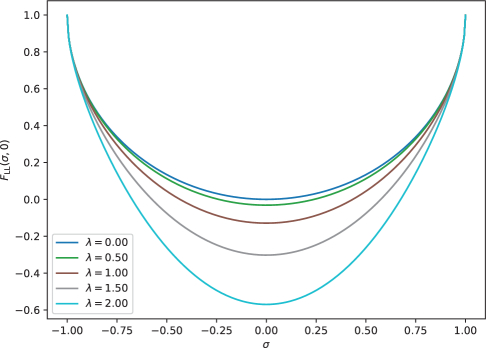
Figure 2. The universal density functional $F_{\mathrm{LL}}(\sigma,0)=F_{\mathrm{L}}(\sigma,0)$ in the reduced setting ($N=M=1$) with $t=1$ and for different values of $\lambda$.

We continue by discussing the Euler–Lagrange equation of the constrained optimization problem in analogy to Theorem 3.7.

Theorem 3.18 (Optimality).

Let $\psi\in\mathcal{M}_{\sigma,\xi}$ be an optimizer of $F_{\mathrm{LL}}(\sigma,\xi)$. If $\sigma\neq\pm 1$, there exist unique Lagrange multipliers $E,v,j\in\mathbb{R}$ such that $\psi$ satisfies the strong Schrödinger equation

$$H(v,j)\psi=E\psi$$ (13)

and the second-order condition

$$\langle\chi,H(v,j)\chi\rangle\geq E\|\chi\|^{2}$$

for all $\chi\in\mathcal{T}_{\psi}(\mathcal{M}_{\sigma,\xi})$. Moreover, $\psi$ has internal energy $\langle\psi,H_{0}\psi\rangle=E-v\sigma-j\xi$.

If $\sigma=+1$, then there exists a $n\in\mathbb{N}_{0}$, such that $\widetilde{\psi}^{+}(x)=\psi^{+}(x+\xi)$ ($\psi^{-}\equiv 0$) satisfies the strong Schrödinger equation for the harmonic oscillator instead,

$$-(\widetilde{\psi}^{+})^{\prime\prime}+x^{2}\widetilde{\psi}^{+}=(2n+1)\widetilde{\psi}^{+},$$ (14)

and one has $\langle\psi,H_{0}\psi\rangle=2n+1+\lambda\xi+\xi^{2}$. If $\sigma=-1$, the same result with $\psi^{+}$ and $\psi^{-}$ interchanged follows.

We have omitted the discussion of the optimality conditions for irregular $\sigma$’s in the general case, but now in the $N=M=1$ case, we see that we get a “degenerate” equation 14, which may be viewed as 13 in the decoupling limit $t\to 0$.

Due to the aforementioned spectral properties of the quantum Rabi model, we can say much more about the optimizers than in the general case.

Theorem 3.19 (unique pure-state $v$-representability).

The following properties hold true.

1. (Regular case) If $\sigma\neq\pm 1$ then for every $(\sigma,\xi)$ there exists a unique $(v,j)$ and $\psi\in\mathcal{M}_{\sigma,\xi}$ strictly positive that is the (unique) ground state of $H(v,j)\psi=E(v,j)\psi$. Moreover, this $\psi\in\mathcal{M}_{\sigma,\xi}$ is the (unique) optimizer of $F_{\mathrm{LL}}(\sigma,\xi)$. In other words, every $(\sigma,\xi)$ pair is uniquely pure-state $v$-representable for $\sigma\neq\pm 1$.

2. (Irregular case) If, however, $\sigma=\pm 1$ then $(\sigma,\xi)$ is not $v$-representable.

From this, we immediately obtain that the pure-state and the mixed-state constrained-search functionals coincide.

Proposition 3.20.

There holds $F_{\mathrm{L}}=F_{\mathrm{LL}}$ on $[-1,1]\times\mathbb{R}$ and the functional is differentiable on the regular set $(-1,1)\times\mathbb{R}$.

That $F_{\mathrm{LL}}$ is continuous and even differentiable is in stark contrast with standard DFT, where the corresponding functionals are everywhere discontinuous [Lam07]. However, at $|\sigma|=1$ the non-$v$-representability according to Theorem 3.19 (ii) implies an empty subdifferential which manifests itself with divergent derivatives of $\sigma\mapsto F_{\mathrm{LL}}(\sigma,\xi)$ as $|\sigma|\to 1$. We expect an analogous behavior also in the general case of the multi-mode Dicke model. Figure 2 shows the universal functional $F_{\mathrm{LL}}(\sigma,0)$ obtained from a numerical calculation for different values of the coupling constant $\lambda$.

4. Proofs

The rest of the paper is devoted to proofs.

4.1. Proofs of Section 2.2

Proof of Theorem 2.1.

Let ${\bm{\psi}}$ be a ground state of $\mathbf{H}(\mathbf{v},\mathbf{j})$, and let

$$\psi_{{\bm{\mu}}}^{\bm{\alpha}}(\mathbf{x})=\mu_{\bm{\alpha}}^{M/2}\psi^{\bm{\alpha}}(\mu_{\bm{\alpha}}\mathbf{x})$$

for some $\mu_{\bm{\alpha}}>0$. Then $\|{\bm{\psi}}_{{\bm{\mu}}}\|=1$ and ${\bm{\psi}}_{(1,\ldots,1)}={\bm{\psi}}$. The different terms of $\langle{\bm{\psi}}_{{\bm{\mu}}},\mathbf{H}(\mathbf{v},\mathbf{j}){\bm{\psi}}_{{\bm{\mu}}}\rangle$ read

$$\|\gradient{\bm{\psi}}_{{\bm{\mu}}}\|^{2} =\sum_{\bm{\alpha}}\mu_{\bm{\alpha}}^{2}\|\gradient\psi^{\bm{\alpha}}\|^{2},$$

$$\|\mathbf{x}{\bm{\psi}}_{{\bm{\mu}}}\|^{2} =\sum_{\bm{\alpha}}\mu_{\bm{\alpha}}^{-2}\|\mathbf{x}\psi^{\bm{\alpha}}\|^{2},$$

$$\langle{\bm{\psi}}_{{\bm{\mu}}},\mathbf{x}\cdot{\bm{\Lambda}}{\bm{\sigma}}_{z}{\bm{\psi}}_{{\bm{\mu}}}\rangle =\sum_{m=1}^{M}\sum_{n=1}^{N}\Lambda_{mn}\sum_{{\bm{\alpha}}}\mu_{\bm{\alpha}}^{-1}(\sigma_{z}^{n})_{{\bm{\alpha}}{\bm{\alpha}}}\langle\psi^{\bm{\alpha}},x_{m}\psi^{\bm{\alpha}}\rangle,$$

$$\langle{\bm{\psi}}_{{\bm{\mu}}},\mathbf{t}\cdot{\bm{\sigma}}_{x}{\bm{\psi}}_{{\bm{\mu}}}\rangle =\sum_{n=1}^{N}t_{n}\sum_{{\bm{\alpha}},{\bm{\beta}}}(\sigma_{x}^{n})_{{\bm{\alpha}}{\bm{\beta}}}\mu_{\bm{\alpha}}^{M/2}\mu_{\bm{\beta}}^{M/2}\int_{\mathbb{R}^{M}}\overline{\psi^{\bm{\alpha}}(\mu_{\bm{\alpha}}\mathbf{x})}\psi^{\bm{\beta}}(\mu_{\bm{\beta}}\mathbf{x})\,\differential\mathbf{x},$$

$$\langle{\bm{\psi}}_{{\bm{\mu}}},\mathbf{v}\cdot{\bm{\sigma}}_{z}{\bm{\psi}}_{{\bm{\mu}}}\rangle =\sum_{n=1}^{N}v_{n}\sum_{\bm{\alpha}}(\sigma_{z}^{n})_{{\bm{\alpha}}{\bm{\alpha}}}\|\psi^{\bm{\alpha}}\|^{2},$$

$$\langle{\bm{\psi}}_{{\bm{\mu}}},\mathbf{j}\cdot\mathbf{x}{\bm{\psi}}_{{\bm{\mu}}}\rangle =\sum_{m=1}^{N}j_{m}\sum_{{\bm{\alpha}}}\mu_{\bm{\alpha}}^{-1}\langle\psi^{\bm{\alpha}},x_{m}\psi^{\bm{\alpha}}\rangle.$$

The optimality condition

$$0=\frac{\partial}{\partial\mu_{\bm{\beta}}}\Big{|}_{{\bm{\mu}}=(1,\ldots,1)}\langle{\bm{\psi}}_{{\bm{\mu}}},\mathbf{H}(\mathbf{v},\mathbf{j}){\bm{\psi}}_{{\bm{\mu}}}\rangle$$

yields

$$0 =2\|\gradient\psi^{\bm{\beta}}\|^{2}-2\|\mathbf{x}\psi^{\bm{\beta}}\|^{2}-\sum_{n=1}^{N}\sum_{m=1}^{M}\Lambda_{mn}(\sigma_{z}^{n})_{{\bm{\beta}}{\bm{\beta}}}\int_{\mathbb{R}^{M}}x_{m}|\psi^{\bm{\beta}}|^{2}\,\differential\mathbf{x}$$

$$-M\sum_{n=1}^{N}\sum_{\bm{\alpha}}t_{n}(\sigma_{x}^{n})_{{\bm{\alpha}}{\bm{\beta}}}\real\langle\psi^{\bm{\alpha}},\psi^{\bm{\beta}}\rangle$$

$$-\sum_{n=1}^{N}\sum_{\bm{\alpha}}t_{n}(\sigma_{x}^{n})_{{\bm{\alpha}}{\bm{\beta}}}2\real\int_{\mathbb{R}^{M}}\overline{\psi^{\bm{\alpha}}(\mathbf{x})}\mathbf{x}\cdot\gradient\psi^{\bm{\beta}}(\mathbf{x})\,\differential\mathbf{x}$$

$$-\mathbf{j}\cdot{\bm{\xi}}_{\bm{\psi}}.$$

Summation over ${\bm{\beta}}$ and rearranging yields

$$2\|\gradient{\bm{\psi}}\|^{2}-2\|\mathbf{x}{\bm{\psi}}\|^{2}-\langle{\bm{\psi}},\mathbf{x}\cdot{\bm{\Lambda}}{\bm{\sigma}}_{z}{\bm{\psi}}\rangle$$

$$=M\langle{\bm{\psi}},\mathbf{t}\cdot{\bm{\sigma}}_{x}{\bm{\psi}}\rangle+2\real\langle{\bm{\psi}},(\mathbf{t}\cdot{\bm{\sigma}}_{x})(\mathbf{x}\cdot\gradient){\bm{\psi}}\rangle+\mathbf{j}\cdot{\bm{\xi}}_{\bm{\psi}}.$$

Next, we use the family of wavefunctions ${\mathbf{M}}\mapsto{\bm{\psi}}_{\mathbf{M}}(\mathbf{x})=(\det{\mathbf{M}})^{1/2}{\bm{\psi}}({\mathbf{M}}\mathbf{x})$, where ${\mathbf{M}}\in\mathbb{R}^{M\times M}$ is a diagonal matrix with positive entries ${\mathbf{M}}=\operatorname{diag}(\mu_{1},\ldots,\mu_{M})$. We have $\|{\bm{\psi}}_{\mathbf{M}}\|=1$. The optimality condition $\frac{\partial}{\partial\mu_{m}}\langle{\bm{\psi}}_{{\mathbf{M}}},\mathbf{H}(\mathbf{v},\mathbf{j}){\bm{\psi}}_{{\mathbf{M}}}\rangle|_{\mu_{1}=\ldots=\mu_{M}=1}=0$ gives

$$\|\gradient{\bm{\psi}}\|^{2}=\|\mathbf{x}{\bm{\psi}}\|^{2}+\frac{1}{2}\langle{\bm{\psi}},\mathbf{x}\cdot{\bm{\Lambda}}{\bm{\sigma}}_{z}{\bm{\psi}}\rangle+\mathbf{j}\cdot{\bm{\xi}}_{\bm{\psi}}.$$

∎

4.2. Proofs of Section 3.1

Proof of Proposition 3.1.

We say that a subset $S$ of vertices of the $N$-cube $[-1,1]^{N}$ is irregular if $\operatorname{Aff}(S)\neq\mathbb{R}^{N}$, and we say that $S$ is maximally irregular if $\dim\operatorname{Aff}(S)=N-1$. First, any irregular set is contained in some maximally irregular set. Next,

$$\mathcal{R}_{N}=[-1,1]^{N}\setminus\bigcup_{\begin{subarray}{c}S\;\text{maximally}\\ \text{irregular}\end{subarray}}\operatorname{Aff}(S),$$

so that $\mathcal{R}_{N}$ is obtained by successively cutting the convex polytope $[-1,1]^{N}$ with hyperplanes, so $\mathcal{R}_{N}$ splits into open convex polytopes. ∎

To prove Theorems 3.2 and 3.19, we need the following version of the unique continuation property (UCP) [Gar20, Theorem 2.3]. Since the condition on the potential is only locally $L^{2}$, it is fulfilled for the case of the harmonic oscillator potential and the coupling term.

Theorem 4.1 (Strong UCP for systems of equations).

Let ${\mathbf{W}}\in L^{2}_{\rm loc}(\mathbb{R}^{M},\mathbb{C}^{2^{N}\times 2^{N}})$ be such that for every $R>0$ there exists $c_{R}\geq 0$ such that

$$\mathbb{1}_{B_{R}}|W_{{\bm{\alpha}}{\bm{\beta}}}|^{2}\leq\epsilon_{N,M}(-\bm{\Delta})^{\frac{3}{2}-\delta}+c_{R},$$

for all ${\bm{\alpha}},{\bm{\beta}}\in I$ in the sense of quadratic forms, where $\epsilon_{N,M}>0$ are small constants depending on $N$ and $M$ only. Let ${\bm{\psi}}\in H^{2}_{\rm loc}(\mathbb{R}^{M},\mathbb{C}^{2^{N}})$ be a weak solution to

$$(-\bm{\Delta}\mathbb{1}_{\mathbb{C}^{2^{N}}}+{\mathbf{W}}){\bm{\psi}}=0.$$

If ${\bm{\psi}}$ vanishes on a set of positive measure, then ${\bm{\psi}}\equiv 0$ a.e.

Proof of Theorem 3.2.

Let $E^{(i)}=E(\mathbf{v}^{(i)},\mathbf{j}^{(i)})$. Using the variational principle

$$E^{(1)} =\langle{\bm{\psi}}^{(1)},\mathbf{H}(\mathbf{v}^{(1)},\mathbf{j}^{(1)}){\bm{\psi}}^{(1)}\rangle\leq\langle{\bm{\psi}}^{(2)},\mathbf{H}(\mathbf{v}^{(1)},\mathbf{j}^{(1)}){\bm{\psi}}^{(2)}\rangle$$

$$=\langle{\bm{\psi}}^{(2)},\mathbf{H}(\mathbf{v}^{(2)},\mathbf{j}^{(2)}){\bm{\psi}}^{(2)}\rangle+(\mathbf{v}^{(1)}-\mathbf{v}^{(2)})\cdot{\bm{\sigma}}+(\mathbf{j}^{(1)}-\mathbf{j}^{(2)})\cdot{\bm{\xi}}$$

$$=E^{(2)}+(\mathbf{v}^{(1)}-\mathbf{v}^{(2)})\cdot{\bm{\sigma}}+(\mathbf{j}^{(1)}-\mathbf{j}^{(2)})\cdot{\bm{\xi}}.$$

Moreover,

$$E^{(2)} =\langle{\bm{\psi}}^{(2)},\mathbf{H}(\mathbf{v}^{(2)},\mathbf{j}^{(2)}){\bm{\psi}}^{(2)}\rangle\leq\langle{\bm{\psi}}^{(1)},\mathbf{H}(\mathbf{v}^{(2)},\mathbf{j}^{(2)}){\bm{\psi}}^{(1)}\rangle$$

$$=\langle{\bm{\psi}}^{(1)},\mathbf{H}(\mathbf{v}^{(1)},\mathbf{j}^{(1)}){\bm{\psi}}^{(1)}\rangle+(\mathbf{v}^{(2)}-\mathbf{v}^{(1)})\cdot{\bm{\sigma}}+(\mathbf{j}^{(2)}-\mathbf{j}^{(1)})\cdot{\bm{\xi}}$$

$$=E^{(1)}+(\mathbf{v}^{(2)}-\mathbf{v}^{(1)})\cdot{\bm{\sigma}}+(\mathbf{j}^{(2)}-\mathbf{j}^{(1)})\cdot{\bm{\xi}}.$$

Together, these two bounds imply that there is equality everywhere, hence

$$\langle{\bm{\psi}}^{(1)},\mathbf{H}(\mathbf{v}^{(2)},\mathbf{j}^{(2)}){\bm{\psi}}^{(1)}\rangle =E^{(2)},$$

$$\langle{\bm{\psi}}^{(2)},\mathbf{H}(\mathbf{v}^{(1)},\mathbf{j}^{(1)}){\bm{\psi}}^{(2)}\rangle =E^{(1)},$$

so that $\mathbf{H}(\mathbf{v}^{(2)},\mathbf{j}^{(2)}){\bm{\psi}}^{(1)}=E^{(2)}{\bm{\psi}}^{(1)}$ and $\mathbf{H}({\bm{\psi}}^{(1)},\mathbf{j}^{(1)}){\bm{\psi}}^{(2)}=E^{(1)}{\bm{\psi}}^{(2)}$ again by the variational principle. This means that ${\bm{\psi}}^{(1)}$ is a ground state to $\mathbf{H}(\mathbf{v}^{(2)},\mathbf{j}^{(2)})$ as well as ${\bm{\psi}}^{(2)}$ to $\mathbf{H}(\mathbf{v}^{(1)},\mathbf{j}^{(1)})$. Subtracting $\mathbf{H}(\mathbf{v}^{(i)},\mathbf{j}^{(i)}){\bm{\psi}}^{(i)}=E^{(i)}{\bm{\psi}}^{(i)}$ from these ($i=1,2$), we obtain via 2 that

$$\left((E^{(2)}-E^{(1)})\mathbb{1}_{\mathbb{C}^{2^{N}}}+(\mathbf{v}^{(1)}-\mathbf{v}^{(2)})\cdot{\bm{\sigma}}_{z}+(\mathbf{j}^{(1)}-\mathbf{j}^{(2)})\cdot\mathbf{x}\mathbb{1}_{\mathbb{C}^{2^{N}}}\right)_{{\bm{\alpha}}{\bm{\alpha}}}(\psi^{(i)})^{\bm{\alpha}}(\mathbf{x})\equiv 0$$ (15)

for a.e. $\mathbf{x}\in\mathbb{R}^{M}$ and all ${\bm{\alpha}}\in\{+,-\}^{N}$. Letting ${\mathbf{A}}^{(i)}(\mathbf{x})$ denote the $|I^{(i)}|\times|I^{(i)}|$ matrix in parenthesis with $I^{(i)}$ the set of spinor indices ${\bm{\alpha}}$ for which $(\psi^{(i)})^{\bm{\alpha}}\not\equiv 0$, we can write 15 equivalently as

$$\widetilde{{\bm{\psi}}}^{(i)}(\mathbf{x})\in\ker{\mathbf{A}}^{(i)}(\mathbf{x})$$

for a.e. $\mathbf{x}\in\mathbb{R}^{M}$, where we have set $\widetilde{{\bm{\psi}}}^{(i)}=((\psi^{(i)})^{\bm{\alpha}})_{{\bm{\alpha}}\in I^{(i)}}$. Using Theorem 4.1, the functions $\widetilde{{\bm{\psi}}}^{(i)}:\mathbb{R}^{M}\to\mathbb{C}^{I^{(i)}}$ cannot vanish on open subsets of $\mathbb{R}^{M}$. Hence, we obtain

$$0\in\sigma({\mathbf{A}}^{(i)}(\mathbf{x}))$$ (16)

for a.e. $\mathbf{x}\in\mathbb{R}^{M}$. Since ${\mathbf{A}}(\mathbf{x})$ is simply a diagonal matrix, its spectrum reads

$$\sigma({\mathbf{A}}^{(i)}(\mathbf{x}))=\left\{E^{(2)}-E^{(1)}+\sum_{n=1}^{N}(v^{(1)}_{n}-v_{n}^{(2)})(\sigma_{z}^{n})_{{\bm{\alpha}}{\bm{\alpha}}}+(\mathbf{j}^{(1)}-\mathbf{j}^{(2)})\cdot\mathbf{x}\right\}_{{\bm{\alpha}}\in I^{(i)}}.$$

Relation 16 then implies that there exists a function ${\bm{\chi}}^{(i)}:\mathbb{R}^{M}\to\{\pm 1\}^{N}$ such that $({\mathbf{A}}^{(i)}(\mathbf{x}))_{{\bm{\chi}}^{(i)}(\mathbf{x}),{\bm{\chi}}^{(i)}(\mathbf{x})}=0$ a.e. $\mathbf{x}\in\mathbb{R}^{M}$. In detail,

$$E^{(2)}-E^{(1)}+\sum_{n=1}^{N}(v^{(1)}_{n}-v_{n}^{(2)})(\sigma_{z}^{n})_{{\bm{\chi}}^{(i)}(\mathbf{x}),{\bm{\chi}}^{(i)}(\mathbf{x})}=-(\mathbf{j}^{(1)}-\mathbf{j}^{(2)})\cdot\mathbf{x},$$

where, as a function of $\mathbf{x}$, the l.h.s. is discontinuous or constant while the r.h.s. is continuous and nonconstant for $\mathbf{j}^{(1)}\neq\mathbf{j}^{(2)}$. We deduce that $\mathbf{j}=\mathbf{j}^{(1)}=\mathbf{j}^{(2)}$ and that ${\bm{\chi}}^{(i)}$ is constant, so $\widetilde{{\bm{\psi}}}^{(i)}(\mathbf{x})\in\ker{\mathbf{A}}^{(i)}$. Hence, (15) reduces to

$$\sum_{n=1}^{N}(v^{(1)}_{n}-v_{n}^{(2)})(\sigma_{z}^{n})_{{\bm{\alpha}}{\bm{\alpha}}}=E^{(1)}-E^{(2)},$$

for every ${\bm{\alpha}}$ such that $(\psi^{(i)})^{\bm{\alpha}}\not\equiv 0$ for some $i=1,2$. From this, the statement for the irregular case (ii) follows right away.

Now suppose that ${\bm{\sigma}}$ is regular and put ${\bm{\psi}}={\bm{\psi}}^{(1)}$. The preceding relation can be compactly written as a linear system

$${\mathbf{P}}{\bm{\Omega}}^{\top}(\mathbf{v}^{(1)}-\mathbf{v}^{(2)})=(E^{(1)}-E^{(2)}){\mathbf{P}}\mathbf{e},$$ (17)

where the $N\times 2^{N}$ matrix ${\bm{\Omega}}$ is given by $\Omega_{n,{\bm{\alpha}}}=(\sigma_{z}^{n})_{{\bm{\alpha}}{\bm{\alpha}}}$ and $\mathbf{e}=(1,\ldots,1)\in\mathbb{R}^{2^{N}}$. Also, ${\mathbf{P}}$ is $2^{N}\times 2^{N}$ the orthogonal projector onto the linear hull of

$$\{\mathbf{e}_{\bm{\alpha}}:\psi^{\bm{\alpha}}\not\equiv 0\}=\{\mathbf{e}_{\bm{\alpha}}:\|\psi^{\bm{\alpha}}\|^{2}\neq 0\}.$$

The regularity of ${\bm{\sigma}}\in[-1,1]^{N}$ implies (is in fact equivalent to) that for all $\omega_{\bm{\alpha}}\geq 0$ such that $\sum_{\bm{\alpha}}\omega_{\bm{\alpha}}=1$ and ${\bm{\Omega}}{\bm{\omega}}={\bm{\sigma}}$, we have $\operatorname{Span}\{{\bm{\Omega}}\mathbf{e}_{\bm{\alpha}}:\omega_{\bm{\alpha}}\neq 0\}=\mathbb{R}^{N}$ and $0\in\operatorname{Aff}\{{\bm{\Omega}}\mathbf{e}_{\bm{\alpha}}:\omega_{\bm{\alpha}}\neq 0\}$. We choose ${\bm{\omega}}=(\|\psi^{\bm{\alpha}}\|^{2})_{{\bm{\alpha}}}$ in what follows.

We may distinguish two cases regarding the solvability of 17.

1. If $E^{(1)}=E^{(2)}$, then 17 is equivalent to

   $$(\mathbf{v}^{(1)}-\mathbf{v}^{(2)})\in\ker{\mathbf{P}}{\bm{\Omega}}^{\top}=(\operatorname{ran}{\bm{\Omega}}{\mathbf{P}})^{\perp}.$$

   But $\operatorname{ran}{\bm{\Omega}}{\mathbf{P}}=\operatorname{Span}\{{\bm{\Omega}}\mathbf{e}_{\bm{\alpha}}:\omega_{\bm{\alpha}}\neq 0\}\supseteq\operatorname{Aff}\{{\bm{\Omega}}\mathbf{e}_{\bm{\alpha}}:\omega_{\bm{\alpha}}\neq 0\}=\mathbb{R}^{N}$ by hypothesis, so $\mathbf{v}^{(1)}=\mathbf{v}^{(2)}$.

2. Suppose that $E^{(1)}\neq E^{(2)}$, which we can simply “scale away” in 17. By the Fredholm alternative theorem, ${\mathbf{P}}{\bm{\Omega}}^{\top}\mathbf{u}={\mathbf{P}}\mathbf{e}$ does not have a solution $\mathbf{u}\in\mathbb{R}^{N}$ precisely if

   $${\bm{\Omega}}{\mathbf{P}}\mathbf{y}=\bm{0},\quad\mathbf{y}\cdot{\mathbf{P}}\mathbf{e}\neq 0$$

   does have a solution $\mathbf{y}\in\mathbb{R}^{2^{N}}$. In other words, if and only if there exists $\mathbf{w}\in\operatorname{ran}{\mathbf{P}}$ such that ${\bm{\Omega}}\mathbf{w}=\bm{0}$ and $\mathbf{e}\cdot\mathbf{w}\neq 0$. By scaling this is equivalent to

   $$\sum_{{\bm{\alpha}}:\psi^{\bm{\alpha}}\not\equiv 0}w_{\bm{\alpha}}{\bm{\Omega}}\mathbf{e}_{\bm{\alpha}}=0$$

   for some $w_{\bm{\alpha}}\in\mathbb{R}$ with $\sum_{{\bm{\alpha}}:\psi^{\bm{\alpha}}\not\equiv 0}w_{\bm{\alpha}}=1$. In other words, $\bm{0}\in\operatorname{Aff}\{{\bm{\Omega}}\mathbf{e}_{\bm{\alpha}}:\omega_{\bm{\alpha}}\neq 0\}$, which holds by hypothesis. Since the alternative has a solution, it must be that case (I) holds.

This finishes the proof also for the regular case (i). ∎

4.3. Proofs of Section 3.2

Proof of Theorem 3.3.

For the $N$-representability of a given density pair $({\bm{\sigma}},{\bm{\xi}})\in[-1,1]^{N}\times\mathbb{R}^{M}$ define ${\bm{\psi}}(\mathbf{x})=(2\pi)^{-M/4}e^{-\frac{1}{4}|\mathbf{x}-{\bm{\xi}}|^{2}}\mathbf{c}$, where $\mathbf{c}\in\mathbb{R}^{2^{N}}$ is to be determined. It is clear that ${\bm{\psi}}\in Q_{0}$ and $|\mathbf{c}|^{2}=1$ is required for $\|{\bm{\psi}}\|=1$. The constraint ${\bm{\sigma}}_{\bm{\psi}}={\bm{\sigma}}$ reads $\sigma_{z}^{n}\mathbf{c}\cdot\mathbf{c}=\sigma_{n}$ for $n=1,\ldots,N$. More explicitly,

$$\sum_{\bm{\alpha}}|c^{\bm{\alpha}}|^{2}=1,\quad\text{and}\quad\sum_{\bm{\alpha}}(\sigma_{z}^{n})_{{\bm{\alpha}}{\bm{\alpha}}}|c^{\bm{\alpha}}|^{2}=\sigma_{n}.$$

These two are equivalent to finding a nonnegative solution $\beta^{\bm{\alpha}}=|c^{\bm{\alpha}}|^{2}$ of

$$\mathbf{A}\bm{\beta}=\begin{pmatrix}1\\ {\bm{\sigma}}\end{pmatrix},$$

where $\mathbf{A}$ is an $N+1$ by $2^{N}$ matrix whose first row is $(1,\ldots,1)$ and its $(n+1)$st row is the diagonal of $\sigma_{z}^{n}$. We claim that the convex set $\{1\}\times[-1,1]^{N}$ is contained within the cone generated by $\mathbf{A}$, i.e., $\{\mathbf{A}\mathbf{x}:x_{m}\geq 0\}$. In fact, it is easy to see using the definition of the matrices $\sigma_{z}^{n}$, that the shifted hypercube $\{1\}\times[-1,1]^{N}$ has $2^{N}$ vertices and that the standard basis vectors $\mathbf{e}_{\bm{\alpha}}$ of $\mathbb{R}^{2^{N}}$ are mapped by $\mathbf{A}$ to these vertices. Since $|\mathbf{c}|=1$, the constraint ${\bm{\xi}}_{\bm{\psi}}={\bm{\xi}}$ is also verified. ∎

Proof of Theorem 3.4.

Let $\{{\bm{\psi}}_{j}\}\subset Q_{0}$ be an optimizing sequence for $F_{\mathrm{LL}}({\bm{\sigma}},{\bm{\xi}})$, i.e. $\|{\bm{\psi}}_{j}\|=1$, ${\bm{\sigma}}_{{\bm{\psi}}_{j}}={\bm{\sigma}}$, ${\bm{\xi}}_{{\bm{\psi}}_{j}}={\bm{\xi}}$ and $\langle{\bm{\psi}}_{j},\mathbf{H}_{0}{\bm{\psi}}_{j}\rangle\to F_{\mathrm{LL}}({\bm{\sigma}},{\bm{\xi}})$ as $j\to\infty$. Since $\mathbf{H}_{0}$ is bounded from below, $\{{\bm{\psi}}_{j}\}\subset Q_{0}$ is bounded in the $Q_{0}$-norm. Then, by the Banach–Alaoglu theorem, there exists a subsequence ${\bm{\psi}}_{j}$ (not distinguished in notation) and ${\bm{\psi}}\in Q_{0}$, such that ${\bm{\psi}}_{j}\rightharpoonup{\bm{\psi}}$ weakly in $Q_{0}$. We need to show that ${\bm{\psi}}$ verifies the constraints and its energy did not increase.

Since $\mathbf{V}$ is a trapping potential ($|\mathbf{V}(\mathbf{x})|\to\infty$ as $|\mathbf{x}|\to\infty$), $-\bm{\Delta}+\mathbf{V}$ has compact resolvent, so the embedding $Q_{0}=Q(-\bm{\Delta}+\mathbf{V})\subset L^{2}(\mathbb{R}^{M},\mathbb{C}^{2^{N}})$ is compact. Then ${\bm{\psi}}_{j}\rightharpoonup{\bm{\psi}}$ implies that ${\bm{\psi}}_{j}\to{\bm{\psi}}$ strongly in $L^{2}(\mathbb{R}^{M},\mathbb{C}^{2^{N}})$, and hence $\|{\bm{\psi}}\|=1$ and ${\bm{\sigma}}_{{\bm{\psi}}}={\bm{\sigma}}$. Moreover, by the Cauchy–Schwarz inequality

$$|{\bm{\xi}}_{{\bm{\psi}}}-{\bm{\xi}}| \leq\int_{\mathbb{R}^{M}}|\mathbf{x}||{\bm{\psi}}-{\bm{\psi}}_{j}|^{2}\,\differential\mathbf{x}\leq\left(\int_{\mathbb{R}^{M}}|x|^{2}|{\bm{\psi}}-{\bm{\psi}}_{j}|^{2}\,\differential\mathbf{x}\right)^{1/2}\|{\bm{\psi}}_{j}-{\bm{\psi}}\|\to 0,$$

because the quantity in parenthesis is uniformly bounded due to the fact that $\{{\bm{\psi}}_{j}\}\subset Q_{0}$ is bounded.

Instead of ${\bm{\psi}}\mapsto\langle{\bm{\psi}},\mathbf{H}_{0}{\bm{\psi}}\rangle$ we can consider ${\bm{\psi}}\mapsto\langle{\bm{\psi}},(\mathbf{H}_{0}+C){\bm{\psi}}\rangle$ in the definition of $F_{\mathrm{LL}}({\bm{\sigma}},{\bm{\xi}})$, which would simply yield $F_{\mathrm{LL}}({\bm{\sigma}},{\bm{\xi}})+C$. But now ${\bm{\psi}}\mapsto\langle{\bm{\psi}},(\mathbf{H}_{0}+C){\bm{\psi}}\rangle$ is a closed positive quadratic form, which means it is strongly lower semicontinuous in $Q_{0}$. By Mazur’s theorem it is also weakly l.s.c., hence

$$F_{\mathrm{LL}}({\bm{\sigma}},{\bm{\xi}})+C=\lim_{j\to\infty}\langle{\bm{\psi}}_{j},(\mathbf{H}_{0}+C){\bm{\psi}}_{j}\rangle\geq\langle{\bm{\psi}},(\mathbf{H}_{0}+C){\bm{\psi}}\rangle.$$

But we already know that $\|{\bm{\psi}}\|=1$, so $C$ cancels from the above inequality and we obtain that ${\bm{\psi}}$ is an optimizer for $F_{\mathrm{LL}}({\bm{\sigma}},{\bm{\xi}})$. ∎

Proof of Theorem 3.5.

First, we note that the quadratic energy functional $\mathcal{E}:Q_{0}\to\mathbb{R}$ that enters the definition of $F_{\mathrm{LL}}$ can be written in a convenient form as

$$\mathcal{E}({\bm{\psi}})=\langle{\bm{\psi}},\mathbf{H}_{0}{\bm{\psi}}\rangle=\|\gradient{\bm{\psi}}\|^{2}+\|\mathbf{x}{\bm{\psi}}\|^{2}+\langle{\bm{\psi}},\mathbf{x}\cdot{\bm{\Lambda}}{\bm{\sigma}}_{z}{\bm{\psi}}\rangle-\langle{\bm{\psi}},\mathbf{t}\cdot{\bm{\sigma}}_{x}{\bm{\psi}}\rangle.$$

For part (i), consider the shift operator $\mathcal{D}_{\bm{\zeta}}{\bm{\psi}}(\mathbf{x})={\bm{\psi}}(\mathbf{x}-{\bm{\zeta}})$ for any ${\bm{\zeta}}\in\mathbb{R}^{M}$. Clearly, $\|(\mathcal{D}_{\bm{\zeta}}\psi)^{\bm{\alpha}}\|^{2}=\|\psi^{\bm{\alpha}}\|^{2}$, ${\bm{\sigma}}_{\mathcal{D}_{\bm{\zeta}}{\bm{\psi}}}={\bm{\sigma}}_{\bm{\psi}}$, ${\bm{\xi}}_{\mathcal{D}_{\bm{\zeta}}{\bm{\psi}}}={\bm{\xi}}_{\bm{\psi}}+{\bm{\zeta}}$ and furthermore

$$\mathcal{E}(\mathcal{D}_{\bm{\zeta}}{\bm{\psi}})=\mathcal{E}({\bm{\psi}})+2{\bm{\zeta}}\cdot{\bm{\xi}}+{\bm{\zeta}}\cdot{\bm{\Lambda}}{\bm{\sigma}}+|{\bm{\zeta}}|^{2}.$$

Using $\mathcal{D}_{\bm{\zeta}}{\bm{\psi}}$ as a trial state for $F_{\mathrm{LL}}({\bm{\sigma}},{\bm{\xi}}+{\bm{\zeta}})$, where ${\bm{\psi}}$ is an optimizer for $F_{\mathrm{LL}}({\bm{\sigma}},{\bm{\xi}})$, we obtain the stated relation with a “$\leq$”. Conversely, choosing $\mathcal{D}_{-{\bm{\zeta}}}{\bm{\psi}}$ as a trial state for $F_{\mathrm{LL}}({\bm{\sigma}},{\bm{\xi}})$, where ${\bm{\psi}}$ is an optimizer for $F_{\mathrm{LL}}({\bm{\sigma}},{\bm{\xi}}+{\bm{\zeta}})$, we get the opposite inequality.

Next, for the real-valuedness part of (ii), it is enough to note that we may decouple the real and the imaginary parts of ${\bm{\psi}}$ within the constraints and the energy. The only nontrivial terms are

$$\langle{\bm{\psi}},\mathbf{x}\cdot{\bm{\Lambda}}{\bm{\sigma}}_{z}{\bm{\psi}}\rangle =\sum_{m=1}^{M}\sum_{n=1}^{N}\Lambda_{mn}\langle\real{\bm{\psi}},x_{m}\sigma_{z}^{n}\real{\bm{\psi}}\rangle+\sum_{m=1}^{M}\sum_{n=1}^{N}\Lambda_{mn}\langle\imaginary{\bm{\psi}},x_{m}\sigma_{z}^{n}\imaginary{\bm{\psi}}\rangle$$

and

$$\langle{\bm{\psi}},\mathbf{t}\cdot{\bm{\sigma}}_{x}{\bm{\psi}}\rangle =\sum_{n=1}^{N}t_{n}\langle{\bm{\psi}},\sigma_{x}^{n}{\bm{\psi}}\rangle=\sum_{n=1}^{N}t_{n}\langle\real{\bm{\psi}},\sigma_{x}^{n}\real{\bm{\psi}}\rangle+\sum_{n=1}^{N}t_{n}\langle\imaginary{\bm{\psi}},\sigma_{x}^{n}\imaginary{\bm{\psi}}\rangle,$$

where the mixed terms cancel using the fact that both $\sigma_{z}^{n}$ and $\sigma_{x}^{n}$ are real symmetric. This allows to minimize $\mathcal{E}({\bm{\psi}})=\mathcal{E}(\real{\bm{\psi}})+\mathcal{E}(\imaginary{\bm{\psi}})$ with just $\real{\bm{\psi}}$.

To see the virial relation (iii), we employ the usual scaling argument [LP85]. Consider the family of wavefunctions ${\mathbf{M}}\mapsto{\bm{\psi}}_{\mathbf{M}}(\mathbf{x}):=(\det{\mathbf{M}})^{1/2}{\bm{\psi}}({\mathbf{M}}\mathbf{x})$, where ${\mathbf{M}}\in\mathbb{R}^{M\times M}$ is a diagonal matrix with positive entries ${\mathbf{M}}=\operatorname{diag}(\mu_{1},\ldots,\mu_{M})$ and ${\bm{\psi}}$ is an optimizer for $F_{\mathrm{LL}}({\bm{\sigma}},\bm{0})$. We have $\|{\bm{\psi}}_{\mathbf{M}}\|=1$, ${\bm{\sigma}}_{{\bm{\psi}}_{\mathbf{M}}}={\bm{\sigma}}$ and ${\bm{\xi}}_{{\bm{\psi}}_{\mathbf{M}}}={\mathbf{M}}^{-1}{\bm{\xi}}=0$. Moreover,

$$\mathcal{E}({\bm{\psi}}_{\mathbf{M}})=\|{\mathbf{M}}\gradient{\bm{\psi}}\|^{2}+\|{\mathbf{M}}^{-1}\mathbf{x}{\bm{\psi}}\|^{2}+\langle{\bm{\psi}},{\mathbf{M}}^{-1}\mathbf{x}\cdot{\bm{\Lambda}}{\bm{\sigma}}_{z}{\bm{\psi}}\rangle-\langle{\bm{\psi}},\mathbf{t}\cdot{\bm{\sigma}}_{x}{\bm{\psi}}\rangle.$$

Since ${\bm{\psi}}$ is an optimizer, we necessarily have $\frac{\partial}{\partial\mu_{m}}\mathcal{E}({\bm{\psi}}_{\mathbf{M}})|_{\mu_{1}=\ldots=\mu_{M}=1}=0$, i.e., with $\mathbf{e}_{m}$ the $m$th unit vector in $\mathbb{R}^{M}$,

$$0=2\|\partial_{x_{m}}{\bm{\psi}}\|^{2}-2\|x_{m}{\bm{\psi}}\|^{2}-\langle{\bm{\psi}},x_{m}\mathbf{e}_{m}\cdot{\bm{\Lambda}}{\bm{\sigma}}_{z}{\bm{\psi}}\rangle,$$

from which the stated formula follows.

To prove (iv), fix $m$ and consider the shifted family

$$s\mapsto{\bm{\psi}}_{s}(\mathbf{x})=(\psi^{\bm{\alpha}}(\mathbf{x}+sc^{\bm{\alpha}}\mathbf{e}_{m}))_{{\bm{\alpha}}},$$

where ${\bm{\psi}}$ is a real-valued optimizer (according to (ii)) for $F_{\mathrm{LL}}({\bm{\sigma}},{\bm{\xi}})$ and $c^{\bm{\alpha}}$ is given by

$$c^{\bm{\alpha}}=\sum_{n=1}^{N}\Lambda_{mn}(\sigma_{z}^{n})_{{\bm{\alpha}}{\bm{\alpha}}}-\sum_{n=1}^{N}\Lambda_{mn}\sigma_{n}$$

so that

$$\sum_{{\bm{\alpha}}}c^{\bm{\alpha}}\|\psi^{\bm{\alpha}}\|^{2}=0.$$

We have $\|{\bm{\psi}}_{s}\|=1$, ${\bm{\sigma}}_{{\bm{\psi}}_{s}}={\bm{\sigma}}$ and

$${\bm{\xi}}_{{\bm{\psi}}_{s}} =\sum_{{\bm{\alpha}}}\int_{\mathbb{R}^{M}}\mathbf{x}|\psi^{\bm{\alpha}}(\mathbf{x}+sc^{\bm{\alpha}}\mathbf{e}_{m})|^{2}\,\differential\mathbf{x}=\sum_{{\bm{\alpha}}}\int_{\mathbb{R}^{M}}(\mathbf{x}-sc^{\bm{\alpha}}\mathbf{e}_{m})|\psi^{\bm{\alpha}}|^{2}\,\differential\mathbf{x}={\bm{\xi}}$$

by construction. Now

$$\mathcal{E}({\bm{\psi}}_{s}) =\langle{\bm{\psi}}_{s},\mathbf{H}_{0}{\bm{\psi}}_{s}\rangle=\|\gradient{\bm{\psi}}\|^{2}+\sum_{\bm{\alpha}}\int_{\mathbb{R}^{M}}|\mathbf{x}-sc^{\bm{\alpha}}\mathbf{e}_{m}|^{2}|\psi^{\bm{\alpha}}|^{2}\,\differential\mathbf{x}$$

$$+\sum_{n^{\prime}=1}^{N}\sum_{m^{\prime}=1}^{M}\Lambda_{m^{\prime}n^{\prime}}\sum_{{\bm{\alpha}}}\int_{\mathbb{R}^{M}}(x_{m^{\prime}}-sc^{\bm{\alpha}}\delta_{mm^{\prime}})(\sigma_{z}^{n^{\prime}})_{{\bm{\alpha}}{\bm{\alpha}}}|\psi^{\bm{\alpha}}|^{2}\,\differential\mathbf{x}$$

$$-\sum_{n^{\prime}=1}^{N}t_{n^{\prime}}\sum_{{\bm{\alpha}},{\bm{\beta}}}(\sigma_{x}^{n^{\prime}})_{{\bm{\beta}}{\bm{\alpha}}}\int_{\mathbb{R}^{M}}\psi^{\bm{\beta}}(\mathbf{x}+sc^{\bm{\beta}}\mathbf{e}_{m})\psi^{\bm{\alpha}}(\mathbf{x}+sc^{\bm{\alpha}}\mathbf{e}_{m})\,\differential\mathbf{x},$$

and the optimality condition $\frac{\differential}{\differential s}\mathcal{E}({\bm{\psi}}_{s})|_{s=0}=0$ implies

$$0= -2\sum_{\bm{\alpha}}\int_{\mathbb{R}^{M}}c^{\bm{\alpha}}x_{m}|\psi^{\bm{\alpha}}|^{2}\,\differential\mathbf{x}-\sum_{n^{\prime}=1}^{N}\Lambda_{mn^{\prime}}\sum_{{\bm{\alpha}}}(\sigma_{z}^{n^{\prime}})_{{\bm{\alpha}}{\bm{\alpha}}}c^{\bm{\alpha}}\|\psi^{\bm{\alpha}}\|^{2}$$

$$-\sum_{n^{\prime}=1}^{N}t_{n^{\prime}}\sum_{{\bm{\alpha}},{\bm{\beta}}}(\sigma_{x}^{n^{\prime}})_{{\bm{\beta}}{\bm{\alpha}}}c^{\bm{\beta}}\int_{\mathbb{R}^{M}}(\partial_{x_{m}}\psi^{\bm{\beta}}(\mathbf{x}))\psi^{\bm{\alpha}}(\mathbf{x})\,\differential\mathbf{x}$$

$$-\sum_{n^{\prime}=1}^{N}t_{n^{\prime}}\sum_{{\bm{\alpha}},{\bm{\beta}}}(\sigma_{x}^{n^{\prime}})_{{\bm{\beta}}{\bm{\alpha}}}c^{\bm{\alpha}}\int_{\mathbb{R}^{M}}\psi^{\bm{\beta}}(\mathbf{x})(\partial_{x_{m}}\psi^{\bm{\alpha}}(\mathbf{x}))\,\differential\mathbf{x}.$$

Using the definition of $c^{\bm{\alpha}}$ and the symmetry of $\sigma_{x}^{n}$ for the last term, we find

$$0= -2\sum_{\bm{\alpha}}\sum_{n=1}^{N}\int_{\mathbb{R}^{M}}x_{m}\Lambda_{mn}(\sigma_{z}^{n})_{{\bm{\alpha}}{\bm{\alpha}}}|\psi^{\bm{\alpha}}|^{2}\,\differential\mathbf{x}+2\sum_{n=1}^{N}\Lambda_{mn}\sigma_{n}\sum_{\bm{\alpha}}\int_{\mathbb{R}^{M}}x_{m}|\psi^{\bm{\alpha}}|^{2}\,\differential\mathbf{x}$$

$$-\sum_{n,n^{\prime}=1}^{N}\Lambda_{mn^{\prime}}\Lambda_{mn}\sum_{{\bm{\alpha}}}(\sigma_{z}^{n^{\prime}})_{{\bm{\alpha}}{\bm{\alpha}}}(\sigma_{z}^{n})_{{\bm{\alpha}}{\bm{\alpha}}}\|\psi^{\bm{\alpha}}\|^{2}+\left(\sum_{n=1}^{N}\Lambda_{mn}\sigma_{n}\right)^{2}$$

$$-2\sum_{n,n^{\prime}=1}^{N}t_{n^{\prime}}\Lambda_{mn}\sum_{{\bm{\alpha}},{\bm{\beta}}}(\sigma_{x}^{n^{\prime}})_{{\bm{\beta}}{\bm{\alpha}}}\left((\sigma_{z}^{n})_{{\bm{\beta}}{\bm{\beta}}}-\sigma_{n}\right)\int_{\mathbb{R}^{M}}(\partial_{x_{m}}\psi^{\bm{\beta}}(\mathbf{x}))\psi^{\bm{\alpha}}(\mathbf{x})\,\differential\mathbf{x}$$

from which

$$0= -2\langle{\bm{\psi}},x_{m}\mathbf{e}_{m}\cdot{\bm{\Lambda}}{\bm{\sigma}}_{z}{\bm{\psi}}\rangle+2\sum_{n=1}^{N}\xi_{m}\Lambda_{mn}\sigma_{n}$$

$$-\sum_{n,n^{\prime}=1}^{N}\Lambda_{mn^{\prime}}\Lambda_{mn}\langle\sigma_{z}^{n^{\prime}}{\bm{\psi}},\sigma_{z}^{n}{\bm{\psi}}\rangle+\left(\sum_{n=1}^{N}\Lambda_{mn}\sigma_{n}\right)^{2}$$

$$-2\sum_{n,n^{\prime}=1}^{N}t_{n^{\prime}}\Lambda_{mn}\langle\sigma_{x}^{n^{\prime}}{\bm{\psi}},(\sigma_{z}^{n}-\sigma_{n})\partial_{x_{m}}{\bm{\psi}}\rangle.$$

The statement then follows from summation over $m$. ∎

Proof of Lemma 3.6.

Consider the smooth map $\mathbf{f}:Q_{0}\to\mathbb{R}^{N+M+1}$ given by

$$\mathbf{f}({\bm{\psi}})=(\|{\bm{\psi}}\|^{2},{\bm{\sigma}}_{\psi},{\bm{\xi}}_{\bm{\psi}}).$$

Then $\mathbf{f}^{-1}(1,{\bm{\sigma}},{\bm{\xi}})=\mathcal{M}_{{\bm{\sigma}},{\bm{\xi}}}$. Note that

$$\mathbf{f}^{\prime}({\bm{\psi}}){\bm{\chi}}=2(\langle{\bm{\psi}},{\bm{\chi}}\rangle,\langle\sigma_{z}^{1}{\bm{\psi}},{\bm{\chi}}\rangle,\ldots,\langle\sigma_{z}^{N}{\bm{\psi}},{\bm{\chi}}\rangle,\langle x_{1}{\bm{\psi}},{\bm{\chi}}\rangle,\ldots,\langle x_{M}{\bm{\psi}},{\bm{\chi}}\rangle).$$

We claim that the differential $(\differential\mathbf{f})_{\bm{\psi}}:Q_{0}\simeq\mathcal{T}_{\bm{\psi}}(Q_{0})\to\mathcal{T}_{(1,{\bm{\sigma}},{\bm{\xi}})}(\mathbb{R}^{N+M+1})\simeq\mathbb{R}^{N+M+1}$ of $\mathbf{f}$ at any ${\bm{\psi}}\in\mathbf{f}^{-1}(1,{\bm{\sigma}},{\bm{\xi}})$ is surjective. To see this, we show that the functions

$$\{{\bm{\psi}}\}\cup\{\sigma_{z}^{1}{\bm{\psi}},\ldots,\sigma_{z}^{N}{\bm{\psi}}\}\cup\{x_{1}{\bm{\psi}},\ldots,x_{M}{\bm{\psi}}\}$$

are linearly independent. Assume for contradiction that there are coefficients $a_{0}$, $a_{1},\ldots,a_{N}\in\mathbb{R}$ and $b_{1},\ldots,b_{M}\in\mathbb{R}$ (not all zero) such that

$$\left(a_{0}+\sum_{n=1}^{N}a_{n}(\sigma_{z}^{n})_{{\bm{\alpha}}{\bm{\alpha}}}+\sum_{m=1}^{M}b_{m}x_{m}\right)\psi^{\bm{\alpha}}(\mathbf{x})=0$$ (18)

for all $\mathbf{x}\in\mathbb{R}^{M}$ and ${\bm{\alpha}}\in\{+,-\}^{N}$. Differentiating 18 with respect to $x_{p}$, $p=1,\ldots,M$, we find

$$\left(a_{0}+\sum_{n=1}^{N}a_{n}(\sigma_{z}^{n})_{{\bm{\alpha}}{\bm{\alpha}}}+\sum_{m=1}^{M}b_{m}x_{m}\right)\partial_{x_{p}}\psi^{\bm{\alpha}}(\mathbf{x})=-b_{p}\psi^{\bm{\alpha}}(\mathbf{x}).$$ (19)

We can assume that $b_{p}\neq 0$ for at least one $p$, since if $b_{1}=\ldots=b_{M}=0$, then 18 implies

$${\mathbf{P}}{\bm{\Omega}}^{\top}\mathbf{a}=a_{0}{\mathbf{P}}\mathbf{e},$$

using the same notations as in the Hohenberg–Kohn theorem’s proof, from which $a_{0}=0$ and $\mathbf{a}=\bm{0}$ follows by the same argument using the regularity of ${\bm{\sigma}}$.

Plugging 19 into 18, we find

$$\left(a_{0}+\sum_{n=1}^{N}a_{n}(\sigma_{z}^{n})_{{\bm{\alpha}}{\bm{\alpha}}}+\sum_{m=1}^{M}b_{m}x_{m}\right)^{2}\partial_{x_{p}}\psi^{\bm{\alpha}}(\mathbf{x})=0$$

for all $\mathbf{x}\in\mathbb{R}^{M}$ and $p=1,\ldots,M$ such that $b_{p}\neq 0$. Taking the inner product with $\partial_{x_{p}}\psi^{\bm{\alpha}}(\mathbf{x})$, we find

$$\left(a_{0}+\sum_{n=1}^{N}a_{n}(\sigma_{z}^{n})_{{\bm{\alpha}}{\bm{\alpha}}}+\sum_{m=1}^{M}b_{m}x_{m}\right)\partial_{x_{p}}\psi^{\bm{\alpha}}(\mathbf{x})=0.$$

Using 19, we find $b_{p}\partial_{x_{p}}\psi^{\bm{\alpha}}(\mathbf{x})=0$. Because ${\bm{\psi}}\neq\bm{0}$ and ${\bm{\psi}}$ is square-integrable, $\gradient{\bm{\psi}}(\mathbf{x})$ must be nonzero on a set of positive measure. But then $b_{p}=0$ which is a contradiction.

Therefore, $(1,{\bm{\sigma}},{\bm{\xi}})$ is a regular value of $\mathbf{f}$. We conclude using the submersion theorem (see e.g. [AMR88, Theorem 3.5.4]) that $\mathcal{M}_{{\bm{\sigma}},{\bm{\xi}}}$ is a closed submanifold of $Q_{0}$, which shows (i), and that the tangent space of $\mathcal{M}_{{\bm{\sigma}},{\bm{\xi}}}$ is given by $\mathcal{T}_{\bm{\psi}}(\mathcal{M}_{{\bm{\sigma}},{\bm{\xi}}})=\ker(\differential\mathbf{f})_{\bm{\psi}}$, from which the stated formulas in (ii) and (iii) follow easily. ∎

Proof of Theorem 3.7.

Let $\mathcal{E}({\bm{\psi}})=\langle{\bm{\psi}},\mathbf{H}_{0}{\bm{\psi}}\rangle$, then the criticality condition reads

$$0=(\differential\mathcal{E}|_{\mathcal{M}_{{\bm{\sigma}},{\bm{\xi}}}})_{\bm{\psi}}({\bm{\chi}})=\langle{\bm{\chi}},\mathbf{H}_{0}{\bm{\psi}}\rangle$$ (20)

for all ${\bm{\chi}}\in\mathcal{T}_{\bm{\psi}}(\mathcal{M}_{{\bm{\sigma}},{\bm{\xi}}})$. In other words, the linear functional $\mathbf{H}_{0}{\bm{\psi}}\in Q_{0}^{*}$ vanishes on $\mathcal{T}_{\bm{\psi}}(\mathcal{M}_{{\bm{\sigma}},{\bm{\xi}}})\subset Q_{0}$. Using the Hahn–Banach theorem, we may extend $\mathbf{H}_{0}{\bm{\psi}}$ to $L^{2}(\mathbb{R}^{M},\mathbb{C}^{2^{N}})$. Denoting the Riesz representation of the extended $\mathbf{H}_{0}{\bm{\psi}}$ with the same expression, $\mathbf{H}_{0}{\bm{\psi}}\in L^{2}(\mathbb{R}^{M},\mathbb{C}^{2^{N}})$ holds, so 20 is simply an $L^{2}$-inner product using the fact that the embedding $L^{2}\subset Q_{0}^{*}$ is continuous. We obtain

$$\mathbf{H}_{0}{\bm{\psi}}\in\mathcal{T}_{\bm{\psi}}(\mathcal{M}_{{\bm{\sigma}},{\bm{\xi}}})^{\perp},$$ (21)

where the orthogonal complement is with respect to the $L^{2}$-inner product. Using Lemma 3.6 (iii), 21 implies that there exists Lagrange multipliers $E\in\mathbb{R}$, $\mathbf{v}\in\mathbb{R}^{N}$ and $\mathbf{j}\in\mathbb{R}^{M}$ such that

$$\mathbf{H}_{0}{\bm{\psi}}=E{\bm{\psi}}-\mathbf{v}\cdot{\bm{\sigma}}_{z}{\bm{\psi}}-\mathbf{j}\cdot\mathbf{x}{\bm{\psi}},$$

as stated.

To show the second order condition 6, let ${\bm{\gamma}}:(-1,1)\to\mathcal{M}_{{\bm{\sigma}},{\bm{\xi}}}$ be a $C^{2}$-curve such that ${\bm{\gamma}}(0)={\bm{\psi}}$ and $\dot{{\bm{\gamma}}}(0)={\bm{\chi}}$. Differentiating the constraints $\|{\bm{\gamma}}(t)\|^{2}=1$, ${\bm{\sigma}}_{{\bm{\gamma}}(t)}={\bm{\sigma}}$ and ${\bm{\xi}}_{{\bm{\gamma}}(t)}={\bm{\xi}}$ twice, we obtain

$$2\real\langle\ddot{{\bm{\gamma}}}(0),{\bm{\psi}}\rangle =-2\|{\bm{\chi}}\|^{2},$$ (22)

$$2\real\langle\ddot{{\bm{\gamma}}}(0),{\bm{\sigma}}_{z}^{n}{\bm{\psi}}\rangle =-2\langle{\bm{\chi}},{\bm{\sigma}}_{z}^{n}{\bm{\chi}}\rangle\quad(n=1,\ldots,N),$$

$$2\real\langle\ddot{{\bm{\gamma}}}(0),x_{m}{\bm{\psi}}\rangle =-2\langle{\bm{\chi}},x_{m}{\bm{\chi}}\rangle\quad(m=1,\ldots,M).$$

We have

$$(\differential^{2}\mathcal{E})_{\bm{\psi}}({\bm{\chi}},{\bm{\chi}}) =\frac{\differential^{2}}{\differential t^{2}}\Big{|}_{0}\langle{\bm{\gamma}}(t),\mathbf{H}_{0}{\bm{\gamma}}(t)\rangle=2\langle{\bm{\chi}},\mathbf{H}_{0}{\bm{\chi}}\rangle+2\real\langle\ddot{{\bm{\gamma}}}(0),\mathbf{H}_{0}{\bm{\psi}}\rangle.$$

Using $\mathbf{H}(\mathbf{v},\mathbf{j})=\mathbf{H}_{0}+\mathbf{v}\cdot{\bm{\sigma}}_{z}+\mathbf{j}\cdot\mathbf{x}$, we get

$$(\differential^{2}\mathcal{E})_{\bm{\psi}}({\bm{\chi}},{\bm{\chi}}) =2\langle{\bm{\chi}},\mathbf{H}(\mathbf{v},\mathbf{j}){\bm{\chi}}\rangle+2\real\langle\ddot{{\bm{\gamma}}}(0),\mathbf{H}(\mathbf{v},\mathbf{j}){\bm{\psi}}\rangle$$

$$-2\sum_{n=1}^{N}v_{n}\langle{\bm{\chi}},{\bm{\sigma}}_{z}^{n}{\bm{\chi}}\rangle-2\sum_{m=1}^{M}j_{m}\langle{\bm{\chi}},x_{m}{\bm{\chi}}\rangle$$

$$-2\real\sum_{n=1}^{N}v_{n}\langle\ddot{{\bm{\gamma}}}(0),{\bm{\sigma}}_{z}^{n}{\bm{\psi}}\rangle-2\real\sum_{m=1}^{M}j_{m}\langle\ddot{{\bm{\gamma}}}(0),x_{m}{\bm{\psi}}\rangle$$

$$=2\langle{\bm{\chi}},(\mathbf{H}(\mathbf{v},\mathbf{j})-E){\bm{\chi}}\rangle,$$

for all ${\bm{\chi}}\in\mathcal{T}_{\bm{\psi}}(\mathcal{M}_{{\bm{\sigma}},{\bm{\xi}}})$, where we used 22 to cancel several terms. Since the Hessian needs to be nonnegative at the optimizer ${\bm{\psi}}$, we obtain the stated relation. ∎

Proof of Theorem 3.8.

Similar to the proof of the Hohenberg-Kohn theorem. ∎

To prove Theorem 3.9, we need a well-known lemma.

Lemma 4.2.

[Lio87, Lemma II.2] Let $H$ be a Hilbert space, $A:H\to H$ a self-adjoint operator bounded from below. If $A$ is nonnegative on a subspace of codimension $d$, then $A$ has at most $d$ nonpositive eigenvalues.

Proof.

Let $\mu_{1}\leq\mu_{2}\leq\ldots$ denote the min-max values of $A$. If $A$ has at most $d$ eigenvalues below the bottom of its essential spectrum (which can be $+\infty$), then we are done. Otherwise, $\mu_{1},\ldots,\mu_{d+1}$ are eigenvalues and the max-min formula implies that

$$\mu_{d+1}\geq\inf_{\begin{subarray}{c}u\in W\\ \|u\|=1\end{subarray}}\langle Au,u\rangle\geq 0,$$

where $W\subset H$ is the $d$-codimensional subspace on which $A$ is nonnegative. ∎

Proof of Theorem 3.9.

The condition 6 this implies that $\mathbf{H}(\mathbf{v},\mathbf{j})-E$ is nonnegative on the $(N+M+1)$-codimensional subspace $\mathcal{T}_{\bm{\psi}}(\mathcal{M}_{{\bm{\sigma}},{\bm{\xi}}})$. Moreover, $\langle{\bm{\psi}},(H(\mathbf{v},\mathbf{j})-E){\bm{\psi}}\rangle=0$ by 5 and ${\bm{\psi}}\in\mathcal{T}_{\bm{\psi}}(\mathcal{M}_{{\bm{\sigma}},{\bm{\xi}}})^{\perp}$, so actually $\mathbf{H}(\mathbf{v},\mathbf{j})-E$ is nonnegative on an $(N+M)$-codimensional subspace. Lemma 4.2 then implies that $\mathbf{H}(\mathbf{v},\mathbf{j})-E$ has at most $N+M$ nonpositive eigenvalues. ∎

4.4. Proofs of Section 3.3

Proof of Lemma 3.10.

By virtue of ${\bm{\Lambda}}=0$, the $N$ two-level systems decouple. Thus, the two-level part of the wavefunction can be written as the $N$-fold tensor product of independent two-level wavefunctions, i.e., ${\bm{\psi}}(\mathbf{x})=\bigotimes_{n=1}^{N}\left(\psi^{+}_{n},\,\psi^{-}_{n}\right)^{\top}\in L^{2}(\mathbb{R}^{M},\mathbb{C}^{2^{N}})$. With this simplification, the constraints for an optimizer ${\bm{\psi}}$ can be combined into the equivalent constraints

$$\norm{\psi_{i}^{\pm}}^{2}=\frac{1\pm\sigma_{i}}{2}\left[\prod_{\begin{subarray}{c}n=1\\ n\neq i\end{subarray}}^{N}\left(\norm{\psi_{n}^{+}}^{2}+\norm{\psi_{n}^{-}}^{2}\right)\right]^{-1}.$$

By use of these constraints and the Cauchy–Schwarz inequality it follows that $\langle{\bm{\psi}},\sigma_{x}^{i}{\bm{\psi}}\rangle\leq\sqrt{1-\sigma_{i}^{2}}$. Furthermore, $\norm{\gradient{\bm{\psi}}}^{2}+\norm{\mathbf{x}{\bm{\psi}}}^{2}\geq M$ by the ground state state energy of the independent harmonic oscillators, implying the lower bound $\langle{\bm{\psi}},\mathbf{H}_{0}{\bm{\psi}}\rangle\geq M-\sum_{n=1}^{N}t_{n}\sqrt{1-\sigma_{n}^{2}}.$ It then follows that $F_{\mathrm{LL}}^{0}({\bm{\sigma}},{\bm{\xi}})\geq M-\sum_{n=1}^{N}t_{n}\sqrt{1-\sigma_{n}^{2}}$, and by the displacement rule, Theorem 3.5 (i), that

$$F_{\mathrm{LL}}^{0}({\bm{\sigma}},{\bm{\xi}})\geq M-\sum_{n=1}^{N}t_{n}\sqrt{1-\sigma_{n}^{2}}+|{\bm{\xi}}|^{2}.$$

Similarly to the proof of Theorem 3.3, suppose the trial state $\psi(\mathbf{x})=\pi^{-M/4}e^{-|\mathbf{x}-{\bm{\xi}}|^{2}/2}\mathbf{c}$ with $\mathbf{c}\in\mathbb{C}^{2^{N}}$ left unspecified. Then by the same calculation, it follows that $|\mathbf{c}|^{2}=1$, ${\bm{\xi}}_{\bm{\psi}}={\bm{\xi}}$ and $\langle\mathbf{c},{\bm{\sigma}}_{z}\mathbf{c}\rangle={\bm{\sigma}}$. Furthermore, we have that $\norm{\gradient{\bm{\psi}}}^{2}=\frac{M}{2}$ and $\norm{\mathbf{x}{\bm{\psi}}}^{2}=\frac{M}{2}+|{\bm{\xi}}|^{2}$. In the case ${\bm{\Lambda}}=\bm{0}$, as discussed above, it is sufficient to consider $\mathbf{c}\in\mathbb{C}^{2N}$. Suppose the particular choice of $\mathbf{c}$ in (8), then it immediately follows that the constraints are satisfied, and that $\langle\mathbf{c},\sigma_{x}^{i}\mathbf{c}\rangle=\sqrt{1-\sigma_{i}^{2}}$. Then

$$\langle{\bm{\psi}},\mathbf{H}_{0}{\bm{\psi}}\rangle=M+|{\bm{\xi}}|^{2}-\sum_{n=1}^{N}t_{n}\sqrt{1-\sigma_{n}^{2}},$$

which in fact equals the lower bound for $F^{0}_{\mathrm{LL}}({\bm{\sigma}},{\bm{\xi}})$, i.e., ${\bm{\psi}}$ is a minimizer. ∎

Proof of Lemma 3.11.

For any optimizers ${\bm{\psi}}_{s{\bm{\Lambda}}}$ and ${\bm{\psi}}_{s^{\prime}{\bm{\Lambda}}}$ of $F_{\mathrm{LL}}^{s{\bm{\Lambda}}}({\bm{\sigma}},{\bm{\xi}})$ and $F_{\mathrm{LL}}^{s^{\prime}{\bm{\Lambda}}}({\bm{\sigma}},{\bm{\xi}})$ respectively, we have

$$F_{\mathrm{LL}}^{s^{\prime}{\bm{\Lambda}}}({\bm{\sigma}},{\bm{\xi}}) =\langle{\bm{\psi}}_{s^{\prime}{\bm{\Lambda}}},\mathbf{H}_{0}^{s^{\prime}{\bm{\Lambda}}}{\bm{\psi}}_{s^{\prime}{\bm{\Lambda}}}\rangle\leq\langle{\bm{\psi}}_{s{\bm{\Lambda}}},\mathbf{H}_{0}^{s^{\prime}{\bm{\Lambda}}}{\bm{\psi}}_{s{\bm{\Lambda}}}\rangle$$

$$=\langle{\bm{\psi}}_{s{\bm{\Lambda}}},\mathbf{H}_{0}^{s{\bm{\Lambda}}}{\bm{\psi}}_{s{\bm{\Lambda}}}\rangle+\langle{\bm{\psi}}_{s{\bm{\Lambda}}},\mathbf{x}\cdot(s^{\prime}-s){\bm{\Lambda}}{\bm{\sigma}}_{z}{\bm{\psi}}_{s{\bm{\Lambda}}}\rangle$$

$$=F_{\mathrm{LL}}^{s{\bm{\Lambda}}}({\bm{\sigma}},{\bm{\xi}})+(s^{\prime}-s)\langle{\bm{\psi}}_{s{\bm{\Lambda}}},\mathbf{x}\cdot{\bm{\Lambda}}{\bm{\sigma}}_{z}{\bm{\psi}}_{s{\bm{\Lambda}}}\rangle.$$

This implies that $\langle{\bm{\psi}}_{s{\bm{\Lambda}}},\mathbf{x}\cdot{\bm{\Lambda}}{\bm{\sigma}}_{z}{\bm{\psi}}_{s{\bm{\Lambda}}}\rangle\in\overline{\partial}_{s}F_{\mathrm{LL}}^{s{\bm{\Lambda}}}({\bm{\sigma}},{\bm{\xi}})(s)$. ∎

4.5. Proofs of Section 3.4

Proof of Theorem 3.13.

The proof closely follows the one of Theorem 4.4 in [Lie83]. By shifting $\mathbf{H}_{0}$ to $\mathbf{H}_{0}+C$ as in the proof of Theorem 3.4, we can achieve $\mathbf{H}_{0}+C>0$. Set $\mathbf{h}=\sqrt{\mathbf{H}_{0}+C}$, then $\mathbf{h}^{-1}$ is compact, because the resolvent $(\mathbf{H}_{0}+C)^{-1}$ is. Let $\{{\bm{\Gamma}}_{j}\}\subset\mathcal{D}(Q_{0})$ be a minimizing sequence such that ${\bm{\sigma}}_{{\bm{\Gamma}}_{j}}={\bm{\sigma}}$, ${\bm{\xi}}_{{\bm{\Gamma}}_{j}}={\bm{\xi}}$. Then for any $\varepsilon>0$ there is a $J\in\mathbb{N}$ such that

$$\Tr\mathbf{h}{\bm{\Gamma}}_{j}\mathbf{h}=\Tr\mathbf{h}^{2}{\bm{\Gamma}}_{j}\leq F_{\mathrm{L}}({\bm{\sigma}},{\bm{\xi}})-C+\varepsilon$$

for all $j\geq J$. We will from here on switch to the subsequence indexed by $j\geq J$. The estimate above implies that the sequence $\mathbf{T}_{j}=\mathbf{h}{\bm{\Gamma}}_{j}\mathbf{h}$ is bounded in trace norm and is thus in $\mathfrak{S}_{1}(\mathcal{H})$. Since $\mathfrak{S}_{\infty}(\mathcal{H})^{*}=\mathfrak{S}_{1}(\mathcal{H})$, with the dual pairing $\Tr\mathbf{T}\mathbf{K}$, where $\mathbf{T}\in\mathfrak{S}_{1}(\mathcal{H})$ and $\mathbf{K}\in\mathfrak{S}_{\infty}(\mathcal{H})$, the Banach–Alaoglu theorem implies that there exists $\mathbf{T}\in\mathfrak{S}_{1}(\mathcal{H})$, such that up to a subsequence,

$$\Tr\mathbf{T}_{j}\mathbf{K}\to\Tr\mathbf{T}\mathbf{K}\quad\text{for all}\quad\mathbf{K}\in\mathfrak{S}_{\infty}(\mathcal{H}).$$ (23)

Since $\mathbf{T}\geq 0$, we have $\liminf_{j\to\infty}\Tr(\mathbf{H}_{0}+C){\bm{\Gamma}}_{j}=\liminf_{j\to\infty}\Tr\mathbf{T}_{j}\geq\Tr\mathbf{T}=\Tr(\mathbf{H}_{0}+C){\bm{\Gamma}}$, where we have set ${\bm{\Gamma}}=\mathbf{h}^{-1}\mathbf{T}\mathbf{h}^{-1}$.

We need to prove now that the self-adjoint, positive trace-class operator ${\bm{\Gamma}}$ with finite $\mathbf{H}_{0}$-energy has the right constraints: $\Tr{\bm{\Gamma}}=1$, ${\bm{\sigma}}_{{\bm{\Gamma}}}={\bm{\sigma}}$ and ${\bm{\xi}}_{{\bm{\Gamma}}}={\bm{\xi}}$. First, taking $\mathbf{K}=\mathbf{h}^{-2}$ in 23, we find $1=\Tr{\bm{\Gamma}}_{j}\to\Tr\mathbf{T}\mathbf{h}^{-2}=\Tr{\bm{\Gamma}}$. Next, we put $\mathbf{K}=\mathbf{h}^{-1}\sigma_{z}^{n}\mathbf{h}^{-1}$, from which follows

$$\sigma_{n}=\Tr\sigma_{z}^{n}{\bm{\Gamma}}_{j}=\Tr\mathbf{T}_{j}\mathbf{h}^{-1}\sigma_{z}^{n}\mathbf{h}^{-1}\to\Tr\mathbf{T}\mathbf{h}^{-1}\sigma_{z}^{n}\mathbf{h}^{-1}=\Tr\sigma_{z}^{n}{\bm{\Gamma}},$$

i.e. ${\bm{\sigma}}_{{\bm{\Gamma}}}={\bm{\sigma}}$. Lastly, we choose $\mathbf{K}=\mathbf{h}^{-1}x_{m}\mathbb{1}_{\mathbb{C}^{2^{N}}}\mathbf{h}^{-1}$, which is compact since $x_{m}$ is bounded in $Q_{0}$ and the embedding $Q_{0}\subset\mathcal{H}$ is compact. Then

$$\xi_{m}=\Tr x_{m}{\bm{\Gamma}}_{j}=\Tr\mathbf{T}_{j}\mathbf{h}^{-1}x_{m}\mathbb{1}_{\mathbb{C}^{2^{N}}}\mathbf{h}^{-1}\to\Tr\mathbf{T}\mathbf{h}^{-1}x_{m}\mathbb{1}_{\mathbb{C}^{2^{N}}}\mathbf{h}^{-1}=\Tr x_{m}{\bm{\Gamma}},$$

which finishes the proof. ∎

Proof of Theorem 3.14.

Part (i) can be proven like Theorem 4.4 and Corollary 4.5 in [Lie83] and a similar proof is given here for Theorem 3.13. Thus this will not be repeated here.

For the proof of (ii) we start from the definition of $F_{\mathrm{L}}$,

$$F_{\mathrm{L}}({\bm{\sigma}},{\bm{\xi}})=\inf_{\begin{subarray}{c}{\bm{\Gamma}}\in\mathcal{D}(Q_{0})\\ {\bm{\sigma}}_{\bm{\Gamma}}={\bm{\sigma}}\\ {\bm{\xi}}_{\bm{\Gamma}}={\bm{\xi}}\end{subarray}}\Tr(\mathbf{H}_{0}{\bm{\Gamma}}).$$

Here, ${\bm{\Gamma}}$ can always be written as an (infinite) convex combination of pure-state projectors as in (9). With this and ${\bm{\sigma}}_{j}={\bm{\sigma}}_{{\bm{\psi}}_{j}}$, ${\bm{\xi}}_{j}={\bm{\xi}}_{{\bm{\psi}}_{j}}$ we have

$$\Tr(\mathbf{H}_{0}{\bm{\Gamma}})=\sum_{j}c_{j}\langle{\bm{\psi}}_{j},\mathbf{H}_{0}{\bm{\psi}}_{j}\rangle,\quad{\bm{\sigma}}=\sum_{j}c_{j}{\bm{\sigma}}_{j},\quad{\bm{\xi}}=\sum_{j}c_{j}{\bm{\xi}}_{j},\quad\sum_{j}c_{j}=1.$$

So instead of over all ${\bm{\Gamma}}$, the infimum can be taken first over all $c_{j}\in\mathbb{R}_{+}$, ${\bm{\sigma}}_{j}\in[-1,1]^{N}$, and ${\bm{\xi}}_{j}\in\mathbb{R}^{M}$ under the constraints above before then taking another infimum over all possible pure states that have ${\bm{\sigma}}_{{\bm{\psi}}_{j}}={\bm{\sigma}}_{j}$, ${\bm{\xi}}_{{\bm{\psi}}_{j}}={\bm{\xi}}_{j}$, i.e., they are from the constraint manifold $\mathcal{M}_{{\bm{\sigma}}_{j},{\bm{\xi}}_{j}}$, and further fulfil the constraints from (9). Without denoting all the constraints this leads to

$$F_{\mathrm{L}}({\bm{\sigma}},{\bm{\xi}})=\inf_{{\bm{\sigma}}_{j},{\bm{\xi}}_{j},c_{j}}\sum_{j}c_{j}\inf_{{\bm{\psi}}_{j}\in\mathcal{M}_{{\bm{\sigma}}_{j},{\bm{\xi}}_{j}}}\langle{\bm{\psi}}_{j},\mathbf{H}_{0}{\bm{\psi}}_{j}\rangle=\inf_{{\bm{\sigma}}_{j},{\bm{\xi}}_{j},c_{j}}\sum_{j}c_{j}F_{\mathrm{LL}}({\bm{\sigma}}_{j},{\bm{\xi}}_{j}).$$

Note that we were able to move the convex sum outside of the inner infimum and thus arrive exactly at the definition for $F_{\mathrm{LL}}$. But this expression is nothing else but the convex envelope. Since we now have that $F_{\mathrm{L}}$ is convex and since the existence of an optimizer (Theorem 3.13) also gives that $F_{\mathrm{L}}$ is locally bounded on all of $(-1,1)^{N}\times\mathbb{R}^{M}$, it is also locally Lipschitz on this set.

To see (iii), we use a well-known characterization: $(-\mathbf{v},-\mathbf{j})\in\underline{\partial}F_{\mathrm{L}}({\bm{\sigma}},{\bm{\xi}})$ if and only if the convex functional $({\bm{\sigma}}^{\prime},{\bm{\xi}}^{\prime})\mapsto F_{\mathrm{L}}({\bm{\sigma}}^{\prime},{\bm{\xi}}^{\prime})+\mathbf{v}\cdot{\bm{\sigma}}^{\prime}+\mathbf{j}\cdot{\bm{\xi}}^{\prime}$ has global minimum at $({\bm{\sigma}},{\bm{\xi}})$. By (12), this in turn is equivalent to

$$E(\mathbf{v},\mathbf{j}) =F_{\mathrm{L}}({\bm{\sigma}},{\bm{\xi}})+\mathbf{v}\cdot{\bm{\sigma}}+\mathbf{j}\cdot{\bm{\xi}}$$

$$=\Tr\mathbf{H}_{0}{\bm{\Gamma}}+\mathbf{v}\cdot{\bm{\sigma}}+\mathbf{j}\cdot{\bm{\xi}}=\Tr\mathbf{H}(\mathbf{v},\mathbf{j}){\bm{\Gamma}}$$

for some ${\bm{\Gamma}}\in\mathcal{D}(Q_{0})$ with ${\bm{\sigma}}_{\bm{\Gamma}}={\bm{\sigma}}$ and ${\bm{\xi}}_{{\bm{\Gamma}}}={\bm{\xi}}$.

The last item, (iv), is a direct consequence of how $E$ is given as the transformation of $F_{\mathrm{L}}$ in (12) and the fact that since $F_{\mathrm{L}}$ is both convex and lower semicontinuous it must agree with the back-transformation of $E$. ∎

Proof of Theorem 3.15.

We first show (i). A proof like for Theorem 3.5 (i) is possible here, but we will show another technique that employs the ladder operators $a_{m}^{\dagger},a_{m}$. Define $a_{m}^{\dagger}=(x_{m}-\partial_{x_{m}})/\sqrt{2}$ and $a_{m}=(x_{m}+\partial_{x_{m}})/\sqrt{2}$. Note that we have $[a_{m},a_{m^{\prime}}]=0$ and $[a_{m},a_{m^{\prime}}^{\dagger}]=[a_{m}^{\dagger},a_{m^{\prime}}]=0$ ($m\neq m^{\prime}$), and $[a_{m},a_{m}^{\dagger}]=1$. For any ${\bm{\zeta}}\in\mathbb{C}^{M}$ define the multimode displacement operator

$$D({\bm{\zeta}})=\prod_{m=1}^{M}\exp\left(\frac{\zeta_{m}a_{m}^{\dagger}-\overline{\zeta_{m}}a_{m}}{\sqrt{2}}\right).$$

Clearly, $D({\bm{\zeta}})^{-1}=D(-{\bm{\zeta}})=D({\bm{\zeta}})^{\dagger}$, i.e. $D({\bm{\zeta}})$ is unitary. Moreover,

$$D({\bm{\zeta}})^{\dagger}a_{m}D({\bm{\zeta}}) =a_{m}+\zeta_{m}/\sqrt{2},$$ (24)

$$D({\bm{\zeta}})^{\dagger}a_{m}^{\dagger}D({\bm{\zeta}}) =a_{m}^{\dagger}+\overline{\zeta}_{m}/\sqrt{2}.$$

Notice that ${\bm{\xi}}_{\bm{\Gamma}}$ can be alternatively written as

$$({\bm{\xi}}_{\bm{\Gamma}})_{m}=\Tr\left(\frac{a_{m}+a_{m}^{\dagger}}{\sqrt{2}}\mathring{\Gamma}\right),$$

so that

$${\bm{\xi}}_{D({\bm{\zeta}}){\bm{\Gamma}}D({\bm{\zeta}})^{\dagger}}={\bm{\xi}}_{\bm{\Gamma}}+\real{\bm{\zeta}}.$$

Clearly, $D({\bm{\zeta}})^{\dagger}\sigma_{j}^{n}D({\bm{\zeta}})=\sigma_{j}^{n}$, hence

$${\bm{\sigma}}_{D({\bm{\zeta}}){\bm{\Gamma}}D({\bm{\zeta}})^{\dagger}}={\bm{\sigma}}_{\bm{\Gamma}}.$$

The internal part of the Hamiltonian in terms of ladder operators is

$$\mathbf{H}_{0}=2\sum_{m=1}^{M}\left(a_{m}^{\dagger}a_{m}+\frac{1}{2}\right)+\sum_{m=1}^{M}\sum_{n=1}^{N}\frac{a_{m}+a_{m}^{\dagger}}{\sqrt{2}}\Lambda_{mn}\sigma_{z}^{n}-\sum_{n=1}^{N}t_{n}\sigma_{x}^{n}.$$

Using 24, the individual parts transform as

$$D({\bm{\zeta}})^{\dagger}a_{m}^{\dagger}a_{m}D({\bm{\zeta}}) =(a_{m}^{\dagger}+\overline{\zeta}_{m}/\sqrt{2})(a_{m}+\zeta_{m}/\sqrt{2})$$

$$=a_{m}^{\dagger}a_{m}+\zeta_{m}a_{m}^{\dagger}/\sqrt{2}+\overline{\zeta}_{m}a_{m}/\sqrt{2}+\tfrac{1}{2}|\zeta_{m}|^{2}$$

$$=a_{m}^{\dagger}a_{m}+(\real\zeta_{m})x_{m}+(\imaginary\zeta_{m})\mathrm{i}\partial_{x_{m}}+\tfrac{1}{2}|\zeta_{m}|^{2},$$

$$D({\bm{\zeta}})^{\dagger}\frac{a_{m}+a_{m}^{\dagger}}{\sqrt{2}}\Lambda_{mn}\sigma_{z}^{n}D({\bm{\zeta}}) =\frac{a_{m}+a_{m}^{\dagger}}{\sqrt{2}}\Lambda_{mn}\sigma_{z}^{n}+(\real\zeta_{m})\Lambda_{mn}\sigma_{z}^{n},$$

$$D({\bm{\zeta}})^{\dagger}t_{n}\sigma_{x}^{n}D({\bm{\zeta}}) =t_{n}\sigma_{x}^{n}.$$

Consequently, the expectation value of the internal part of the Hamiltonian transforms as

$$\Tr(\mathbf{H}_{0}D({\bm{\zeta}}){\bm{\Gamma}}D({\bm{\zeta}})^{\dagger})=\Tr\mathbf{H}_{0}{\bm{\Gamma}}+2(\real{\bm{\zeta}})\cdot{\bm{\xi}}_{\bm{\Gamma}}+2(\imaginary{\bm{\zeta}})\cdot\langle\mathrm{i}\gradient\rangle_{{\bm{\Gamma}}}+(\real{\bm{\zeta}})\cdot{\bm{\Lambda}}{\bm{\sigma}}_{\bm{\Gamma}}+|{\bm{\zeta}}|^{2}.$$ (25)

After these preparations, we are ready to prove the stated formula. First, let ${\bm{\Gamma}}$ be an optimizer for $F_{\mathrm{L}}({\bm{\sigma}},{\bm{\xi}})$, and put $D({\bm{\zeta}}){\bm{\Gamma}}D({\bm{\zeta}})^{\dagger}$, ${\bm{\zeta}}\in\mathbb{R}^{M}$, as a trial state for $F_{\mathrm{L}}({\bm{\sigma}},{\bm{\xi}}+{\bm{\zeta}})$, to get

$$F_{\mathrm{L}}({\bm{\sigma}},{\bm{\xi}}+{\bm{\zeta}})\leq F_{\mathrm{L}}({\bm{\sigma}},{\bm{\xi}})+2{\bm{\zeta}}\cdot{\bm{\xi}}+{\bm{\zeta}}\cdot{\bm{\Lambda}}{\bm{\sigma}}+|{\bm{\zeta}}|^{2}.$$

Conversely, let ${\bm{\Gamma}}$ be an optimizer for $F_{\mathrm{L}}({\bm{\sigma}},{\bm{\xi}}+{\bm{\zeta}})$ and put $D(-{\bm{\zeta}}){\bm{\Gamma}}D(-{\bm{\zeta}})^{\dagger}$ as a trial state to $F_{\mathrm{L}}({\bm{\sigma}},{\bm{\xi}})$ to obtain the opposite inequality.

Next, for (ii), note that the complex conjugation ${\bm{\Gamma}}\mapsto\overline{{\bm{\Gamma}}}$ leaves the energy $\Tr\mathbf{H}_{0}{\bm{\Gamma}}$ invariant, which can be easily verified by writing it with the integral kernel $\overline{{\bm{\Gamma}}(\mathbf{x},\mathbf{x}^{\prime})}={\bm{\Gamma}}(\mathbf{x}^{\prime},\mathbf{x})$. Let ${\bm{\Gamma}}$ be an optimizer for $F_{\mathrm{L}}({\bm{\sigma}},{\bm{\xi}})$ and note that $({\bm{\Gamma}}+\overline{{\bm{\Gamma}}})/2$ is a density matrix as well that has same internal energy $F_{\mathrm{L}}({\bm{\sigma}},{\bm{\xi}})$. Since it is real-valued, this proves (ii).

To show (iii), we consider the one-parameter family of scaled density matrices ${\bm{\Gamma}}_{\mathbf{M}}(\mathbf{x},\mathbf{x}^{\prime})=(\det{\mathbf{M}}){\bm{\Gamma}}({\mathbf{M}}\mathbf{x},{\mathbf{M}}\mathbf{x}^{\prime})$ for any diagonal matrix with positive entries ${\mathbf{M}}=\operatorname{diag}(\mu_{1},\ldots,\mu_{M})\in\mathbb{R}^{M\times M}$. If ${\bm{\Gamma}}$ is an optimizer for $F_{\mathrm{L}}({\bm{\sigma}},\bm{0})$ then ${\bm{\sigma}}_{{\bm{\Gamma}}_{{\mathbf{M}}}}={\bm{\sigma}}_{\bm{\Gamma}}={\bm{\sigma}}$ and ${\bm{\xi}}_{{\bm{\Gamma}}_{{\mathbf{M}}}}={\mathbf{M}}^{-1}{\bm{\xi}}_{{\bm{\Gamma}}}=0$. Moreover,

$$\Tr\mathbf{H}_{0}{\bm{\Gamma}}_{{\mathbf{M}}}=\Tr(-{\mathbf{M}}^{2}(\gradient\otimes\gradient){\bm{\Gamma}})+\Tr|{\mathbf{M}}^{-1}\mathbf{x}|^{2}{\bm{\Gamma}}+\Tr({\mathbf{M}}^{-1}\mathbf{x}\cdot{\bm{\Lambda}}{\bm{\sigma}}_{z}{\bm{\Gamma}})-\Tr(\mathbf{t}\cdot{\bm{\sigma}}_{x}{\bm{\Gamma}}).$$

Since ${\bm{\Gamma}}$ is an optimizer, $\frac{\partial}{\partial\mu_{m}}\Tr\mathbf{H}_{0}{\bm{\Gamma}}_{{\mathbf{M}}}|_{\mu_{m}=1}=0$, i.e.,

$$0=2\Tr((-\partial_{x_{m}}^{2}-x_{m}^{2}){\bm{\Gamma}})-\Tr(x_{m}\mathbf{e}_{m}\cdot{\bm{\Lambda}}{\bm{\sigma}}_{z}{\bm{\Gamma}})$$

from which the stated formula follows after summation over $m$.

For (iv), let ${\bm{\Gamma}}$ be an optimizer for $F_{\mathrm{L}}({\bm{\sigma}},{\bm{\xi}})$ and consider $s\mapsto{\bm{\Gamma}}_{s}=D(\mathrm{i}s\mathbf{e}_{m}){\bm{\Gamma}}D(\mathrm{i}s\mathbf{e}_{m})^{\dagger}$ for a fixed $m$. Using 25, we find

$$0=\frac{\differential}{\differential s}\Big{|}_{s=0}\Tr\mathbf{H}_{0}{\bm{\Gamma}}_{s}=2\langle\mathrm{i}\partial_{x_{m}}\rangle_{{\bm{\Gamma}}},$$

as required. ∎

Proof of Proposition 3.16.

Since $\Tr\mathbf{H}(\mathbf{v},\mathbf{j}){\bm{\Gamma}}=E(\mathbf{v},\mathbf{j})$ the ${\bm{\Gamma}}$ is the optimizer in (11) and thus from (12) we have by characterizing the optimizer with the subdifferential that

$$(-\mathbf{v},-\mathbf{j})\in\underline{\partial}F_{\mathrm{L}}({\bm{\sigma}}_{\bm{\Gamma}},{\bm{\xi}}_{\bm{\Gamma}}).$$

Now put in the displacement rule (i) for $F_{\mathrm{L}}({\bm{\sigma}}_{\bm{\Gamma}},{\bm{\xi}}_{\bm{\Gamma}})$ and from differentiation with respect to ${\bm{\xi}}$ directly get

$$-\mathbf{j}={\bm{\Lambda}}{\bm{\sigma}}_{\bm{\Gamma}}+2{\bm{\xi}}_{\bm{\Gamma}},$$

which concludes the proof. The same result can be achieved as a “hypervirial theorem” [Hir60] with respect to the momentum operator $-\mathrm{i}\vnabla$. ∎

4.6. Proofs of Section 3.5

Proof of Theorem 3.17.

For (i), we use the invertible transformation

$$\psi(x)\mapsto\widetilde{\psi}(x)=\begin{pmatrix}\psi^{-}(-x)\\ \psi^{+}(-x)\end{pmatrix}.$$

Then $\|\widetilde{\psi}^{+}\|^{2}=\frac{1-\sigma}{2}$, $\|\widetilde{\psi}^{-}\|^{2}=\frac{1+\sigma}{2}$ and $\xi_{\widetilde{\psi}}=-\xi$ for any $\psi$ such that $\|\psi^{+}\|^{2}=\frac{1+\sigma}{2}$, $\|\psi^{-}\|^{2}=\frac{1-\sigma}{2}$ and $\xi_{\psi}=\xi$. Also, $\langle\widetilde{\psi},H_{0}\widetilde{\psi}\rangle=\langle\psi,H_{0}\psi\rangle$, from which the claim follows.

As for the real-valuedness part of (ii), it is enough to see that the real and imaginary parts of $\psi$ decouple in the expression of the quadratic form $\langle\psi,H\psi\rangle$, and that the minimization can be carried out for the real and imaginary parts separately. This is obvious, except for the term $-t\langle\sigma_{x}\rangle_{\psi}=-2t\real\langle\psi^{+},\psi^{-}\rangle$. But if we write for any admissible $\psi$,

$$2\real\langle\psi^{+},\psi^{-}\rangle=1-\|\psi^{+}-\psi^{-}\|^{2}=1-\|\real\psi^{+}-\real\psi^{-}\|^{2}-\|\imaginary\psi^{+}-\imaginary\psi^{-}\|^{2}$$

using the polarization identity, then real-valuedness follows. To see non-negativity, let $\psi$ be an admissible wavefunction. Define the level sets $A_{+}^{\alpha}=\{x\in\mathbb{R}:\psi^{\alpha}(x)\geq 0\}$ and $A_{-}^{\alpha}=\{x\in\mathbb{R}:\psi^{\alpha}(x)<0\}$. Set

$$\widetilde{\psi}=\begin{cases}\psi&A_{+}^{+}\cap A_{+}^{-}\\ (\psi^{+},-\psi^{-})&A_{+}^{+}\cap A_{-}^{-}\\ (-\psi^{+},\psi^{-})&A_{-}^{+}\cap A_{+}^{-}\\ -\psi&A_{-}^{+}\cap A_{-}^{-}\end{cases}$$

which is non-negative. It is clear that the constraints and all the terms in $\langle\widetilde{\psi},H_{0}\widetilde{\psi}\rangle$ are unchanged except for $-2t\real\langle\widetilde{\psi}^{+},\widetilde{\psi}^{-}\rangle$, which, again by polarization, can be reduced to looking at

$$\|\widetilde{\psi}^{+}-\widetilde{\psi}^{-}\|^{2} =\int_{A_{+}^{+}\cap A_{+}^{-}}|\psi^{+}-\psi^{-}|^{2}+\int_{A_{+}^{+}\cap A_{-}^{-}}|\psi^{+}+\psi^{-}|^{2}$$

$$+\int_{A_{-}^{+}\cap A_{+}^{-}}|\psi^{+}+\psi^{-}|^{2}+\int_{A_{-}^{+}\cap A_{-}^{-}}|\psi^{+}-\psi^{-}|^{2}.$$

Here, the middle two terms did not increase (now these integrands possibly contain a sum of a positive and a negative function) and the other two integrals remained invariant. We deduce that the transformation $\psi\mapsto\widetilde{\psi}$ did not increase the energy.

To see (iii), consider the one-parameter family of wavefunctions $\psi_{\mu}(x)=\sqrt{\mu}\psi(\mu x)$, which has $\|\psi_{\mu}^{+}\|^{2}=\frac{1+\sigma}{2}$, $\|\psi_{\mu}^{-}\|^{2}=\frac{1-\sigma}{2}$ and $\xi_{\psi_{\mu}}=\frac{1}{\mu}\xi_{\psi}$. Moreover,

$$\langle\psi_{\mu},H_{0}\psi_{\mu}\rangle=\int\left[\mu^{2}|\psi^{\prime}|^{2}+\frac{x^{2}}{\mu^{2}}|\psi|^{2}\right]\differential x+\frac{\lambda}{\mu}\int x\left(|\psi^{+}|^{2}-|\psi^{-}|^{2}\right)\differential x-2t\real\langle\psi^{+},\psi^{-}\rangle.$$

But $\frac{\differential}{\differential\mu}|_{\mu=1}\langle\psi_{\mu},H_{0}\psi_{\mu}\rangle=0$ which is equivalent to the stated relation if we further use $\int x\left(|\psi^{+}|^{2}+|\psi^{-}|^{2}\right)\differential x=\xi_{\psi}=\xi$.

Next, for (iv) we use the transformation

$$\psi\mapsto\psi_{s}=\begin{pmatrix}\psi^{+}(x-(1-\sigma)s)\\ \psi^{-}(x+(1+\sigma)s)\end{pmatrix}$$

which is chosen such that it keeps $\sigma_{\psi_{s}}=\sigma_{\psi}=\sigma$, $\xi_{\psi_{s}}=\xi_{\psi}=\xi$ (not zero necessarily zero) constant. We consider the derivative $\partial_{s}\langle H_{0}\rangle_{\psi_{s}}$ that must be zero at $s=0$ if $\psi$ is an optimizer. The parts of $H_{0}$ are,

$$\langle-t\sigma_{x}\rangle_{\psi_{s}} =-2t\int\psi^{+}(x-(1-\sigma)s)\psi^{-}(x+(1-\sigma)s)\,\differential x,$$

$$\langle\lambda\sigma_{z}x\rangle_{\psi_{s}} =\lambda\langle x+(1-\sigma)s\rangle_{\psi^{+}}-\lambda\langle x-(1+\sigma)s\rangle_{\psi^{-}}$$

$$=\lambda(\langle x\rangle_{\psi^{+}}-\langle x\rangle_{\psi^{-}})+\lambda s(1-\sigma^{2}),$$

$$\langle p^{2}\rangle_{\psi_{s}} =\langle p^{2}\rangle_{\psi},$$

$$\langle x^{2}\rangle_{\psi_{s}} =\langle(x+(1-\sigma)s)^{2}\rangle_{\psi^{+}}+\langle(x-(1+\sigma)s)^{2}\rangle_{\psi^{-}}$$

$$=\langle x^{2}\rangle_{\psi}+2s(\langle x\rangle_{\psi^{+}}-\langle x\rangle_{\psi^{-}})-2s\sigma\xi+s^{2}(1+\sigma^{2}).$$

Now the derivative at $s=0$ yields

$$\frac{\differential}{\differential s}\Big{|}_{s=0}\langle H_{0}\rangle_{\psi_{s}}=2 t(1-\sigma)\int(\psi^{+})^{\prime}\psi^{-}-2t(1+\sigma)\int\psi^{+}(\psi^{-})^{\prime}$$

$$+\lambda(1-\sigma^{2})+2\langle x\rangle_{\psi^{+}}-2\langle x\rangle_{\psi^{-}}-2\sigma\xi=0.$$

As $\langle x\rangle_{\psi^{-}}=\xi-\langle x\rangle_{\psi^{+}}$, this yields the stated result. Moreover, if we similarly consider $\frac{\differential^{2}}{\differential s^{2}}\big{|}_{s=0}\langle\psi_{s},H_{0}\psi_{s}\rangle\geq 0$ we find the stated inequality.

Finally, (v) is just a special case of Lemma 3.10. ∎

Proof of Theorem 3.18.

Existence of the Lagrange multipliers in the regular case $\sigma\neq\pm 1$ was already treated in Theorem 3.7, and uniqueness follows from the fact that the functions $\psi$, $\sigma_{z}\psi$ and $x\psi$ are linearly independent.

It remains to consider the irregular case $\sigma=\pm 1$. We only look at $\sigma=+1$, the other case is analogous, and proceed similarly as in the proof of Theorem 3.7. The criticality condition reads $\langle\chi,H_{0}\psi\rangle=0$ with $\psi=(\psi^{+},0)^{\top}$, $\chi=(\chi^{+},0)^{\top}$, $\int\chi^{+}\psi^{+}=0$ and $\int x\chi^{+}\psi^{+}=0$. This implies, by a similar argument as before, that

$$-(\psi^{+})^{\prime\prime}+x^{2}\psi^{+}+\lambda x\psi^{+}=\mu^{+}\psi^{+}+\mu^{0}x\psi^{+}$$

for some unique $\mu^{+},\mu^{0}\in\mathbb{R}$. Rearranging, we get

$$-(\psi^{+})^{\prime\prime}+\left(x+\frac{\lambda-\mu^{0}}{2}\right)^{2}\psi^{+}=\left(\mu^{+}+\frac{(\lambda-\mu^{0})^{2}}{4}\right)\psi^{+}.$$

The constraint $\xi_{\psi}=\xi$ implies that $\xi=-(\lambda-\mu^{0})/2$, or $\mu^{0}=\lambda+2\xi$. From the eigenvalues of the harmonic oscillator, we find $\mu^{+}=2n+1-\xi^{2}$. The stated equation follows by translation. ∎

Proof of Theorem 3.19.

We know from Theorem 3.17 (ii) that there is at least one optimizer $\psi$ of $F_{\mathrm{LL}}(\sigma,\xi)$ which is non-negative. Since for $\sigma\neq\pm 1$ this $\psi$ satisfies the Schrödinger equation 13 with $H(v,j)$ by Theorem 3.18, it is even positive a.e. by the strong UCP (Theorem 4.1). We also have $\exp(-tH(v,j))$ as a positivity improving operator [HH14, NRBW24], which together with steps 3 and 4 in [Chi17] means that the ground-state eigenvector of $H(v,j)$ is strictly positive and non-degenerate. Any excited eigenstate is orthogonal to the ground state and consequently must change sign. Thus the optimizer $\psi$ must also be the unique ground state.

For the uniqueness part, suppose that $\widetilde{\psi}$ is another optimizer of $F_{\mathrm{LL}}(\sigma,\xi)$ with potentials $(\widetilde{v},\widetilde{j})$, then $E(v,j)=E(\widetilde{v},\widetilde{j})+\sigma(v-\widetilde{v})+\xi(j-\widetilde{j})$. We have

$$E(v,j) \leq\langle\widetilde{\psi},H(v,j)\widetilde{\psi}\rangle=E(\widetilde{v},\widetilde{j})+\sigma(v-\widetilde{v})+\xi(j-\widetilde{j})=E(v,j),$$

hence there is equality. Therefore, $\langle\widetilde{\psi},H(v,j)\widetilde{\psi}\rangle=E(v,j)$, so $\widetilde{\psi}$ satisfies $H(v,j)\widetilde{\psi}=E(v,j)\widetilde{\psi}$, which contradicts the fact that the ground state of $H(v,j)$ is unique.

Finally, if $\sigma=\pm 1$ then note that by Theorem 3.18 the $\psi$ corresponding to $(\sigma,\xi)$ must satisfy the Schrödinger equation for the harmonic oscillator 14 and is thus unique. But 14 is not a Schrödinger equation of the form $H(v,j)\psi=E\psi$. More generally, if $H(v,j)\psi=E\psi$ for some $(v,j)$ and $\psi$, then $\psi^{\mp}=0$ implies that $\psi^{\pm}=0$ from the coupling term $-t\sigma_{x}$, $t\neq 0$, so $\psi\equiv 0$, hence $v$-representability does not hold in this case. ∎

Proof of Proposition 3.20.

We start by showing $F_{\mathrm{L}}=F_{\mathrm{LL}}$ on $(-1,1)\times\mathbb{R}$. By Theorem 3.19 (i) the (unique) optimizer of $F_{\mathrm{LL}}(\sigma,\xi)$ is a ground state of $H(v,j)\psi=E(v,j)\psi$ with $\sigma_{\psi}=\sigma$ and $\xi_{\psi}=\xi$. Any ensemble state $\Gamma$ can be written as a convex combination over pure-state projectors onto normalized $\psi_{j}$, i.e., $\Gamma=\sum_{j}c_{j}|\psi_{j}\rangle\langle\psi_{j}|$ with $\sum_{j}c_{j}=1$. With the variational principle for the ground state $\psi$ this means

$$E(v,j) =F_{\mathrm{LL}}(\sigma,\xi)+\sigma v+\xi j=\sum_{j}c_{j}\langle\psi,H(v,j)\psi\rangle$$

$$\leq\sum_{j}c_{j}\langle\psi_{j},H(v,j)\psi_{j}\rangle=\Tr H(v,j)\Gamma=\Tr H_{0}\Gamma+\sigma v+\xi j.$$

Now taking the infimum over all ensemble states $\Gamma$ with $\sigma_{\Gamma}=\sigma$ and $\xi_{\Gamma}=\xi$ yields $F_{\mathrm{LL}}\leq F_{\mathrm{L}}$. Since anyway $F_{\mathrm{L}}\leq F_{\mathrm{LL}}$ we have that $F_{\mathrm{L}}=F_{\mathrm{LL}}$ on $(-1,1)\times\mathbb{R}$. Since further the $(v,j)$ such that $\psi$ is a ground state of $H(v,j)\psi=E(v,j)\psi$ are unique, the subdifferential $\partial F_{\mathrm{L}}(\sigma,\xi)$ is a singleton and thus the functional is automatically differentiable on $(-1,1)\times\mathbb{R}$.

The cases $\sigma=\pm 1$ are now shown separately. First, by Theorem 3.15 (i) shift to $F_{\mathrm{L}}(\sigma,\xi)=F_{\mathrm{L}}(\sigma,0)+\lambda\sigma\xi+\xi^{2}$, then use the property that $F_{\mathrm{L}}(\sigma,0)$ can be evaluated as the infimum over all convex combinations of $F_{\mathrm{L}}(\sigma_{j},0)$ with $\sum_{j}c_{j}\sigma_{j}=\sigma$ and $\sum_{j}c_{j}=1$ [Lie83, Eq. (4.6)]. But if $\sigma=\pm 1$ then also all $\sigma_{j}=\pm 1$, so no non-trivial convex combination is possible and we directly have $F_{\mathrm{L}}(\sigma,0)=F_{\mathrm{LL}}(\sigma,0)$ from which follows $F_{\mathrm{L}}(\sigma,\xi)=F_{\mathrm{LL}}(\sigma,\xi)$ by the displacement rule. ∎

References

- [AMR88] Ralph Abraham, Jerrold E Marsden and Tudor Ratiu “Manifolds, tensor analysis, and applications” Springer, 1988
- [BLZ15] Murray T Batchelor, Zi-Min Li and Huan-Qiang Zhou “Energy landscape and conical intersection points of the driven Rabi model” In J. Phys. A: Math. Theor. 49 IOP Publishing, 2015, pp. 01LT01 DOI: 10.1088/1751-8113/49/1/01LT01
- [BZ15] Murray T. Batchelor and Huan-Qiang Zhou “Integrability versus exact solvability in the quantum Rabi and Dicke models” In Phys. Rev. A 91 American Physical Society (APS), 2015 DOI: 10.1103/physreva.91.053808
- [BSK24] Lucas Borges, Thomas Schnappinger and Markus Kowalewski “Extending the Tavis–Cummings model for molecular ensembles – Exploring the effects of dipole self energies and static dipole moments” In arXiv preprint: 2404.10680, 2024 DOI: doi.org/10.1063/5.0214362
- [Bra11] D. Braak “Integrability of the Rabi Model” In Physical Review Letters 107 American Physical Society (APS), 2011 DOI: 10.1103/physrevlett.107.100401
- [Bra13] D. Braak “Solution of the Dicke model for N=3” In J. Phys. B: At. Mol. Opt. Phys. 46 IOP Publishing, 2013, pp. 224007 DOI: 10.1088/0953-4075/46/22/224007
- [Bra15] D. Braak “Analytical Solutions of Basic Models in Quantum Optics” In Applications + Practical Conceptualization + Mathematics = fruitful Innovation Springer, 2015, pp. 75–92 DOI: 10.1007/978-4-431-55342-7˙7
- [CF23] “Density Functional Theory: Modeling, Mathematical Analysis, Computational Methods, and Applications” Springer, 2023
- [Chi17] Francesco Chini “Uniqueness of the ground state” Accessed: 01-07-2024, 2017 URL: https://www.nielsbenedikter.de/advmaphys2/ground_state.pdf
- [dCdAdQ16] Bruno Carneiro Cunha, Manuela Carvalho Almeida and Amilcar Rabelo Queiroz “On the existence of monodromies for the Rabi model” In J. Phys. A: Math. Theor. 49 IOP Publishing, 2016, pp. 194002 DOI: 10.1088/1751-8113/49/19/194002
- [DG12] Reiner M Dreizler and Eberhard KU Gross “Density functional theory: An approach to the quantum many-body problem” Springer, 2012
- [Ebb16] Thomas W Ebbesen “Hybrid light–matter states in a molecular and material science perspective” In Acc. Chem. Res. 49 ACS Publications, 2016, pp. 2403–2412 DOI: 10.1021/acs.accounts.6b00295
- [Esc03] Helmut Eschrig “The fundamentals of density functional theory” Springer, 2003
- [FWR+19] Johannes Flick, Davis M Welakuh, Michael Ruggenthaler, Heiko Appel and Angel Rubio “Light–matter response in nonrelativistic quantum electrodynamics” In ACS Photonics 6 ACS Publications, 2019, pp. 2757–2778 DOI: 10.1021/acsphotonics.9b00768
- [GCE21] Francisco J Garcia-Vidal, Cristiano Ciuti and Thomas W Ebbesen “Manipulating matter by strong coupling to vacuum fields” In Science 373 American Association for the Advancement of Science, 2021, pp. eabd0336 DOI: 10.1126/science.abd0336
- [Gar20] Louis Garrigue “Unique Continuation for Many-Body Schrödinger Operators and the Hohenberg–Kohn Theorem. II. The Pauli Hamiltonian” In Doc. Math. 25, 2020, pp. 869–898 DOI: 10.4171/DM/765
- [GR13] Walter Greiner and Joachim Reinhardt “Field quantization” Springer, 2013
- [HDC15] Shu He, Liwei Duan and Qing-Hu Chen “Exact solvability, non-integrability, and genuine multipartite entanglement dynamics of the Dicke model” In New J. Phys. 17 IOP Publishing, 2015, pp. 043033 DOI: 10.1088/1367-2630/17/4/043033
- [HH14] Masao Hirokawa and Fumio Hiroshima “Absence of energy level crossing for the ground state energy of the Rabi model” In Comm. Stoch. Anal. 8 Louisiana State University Libraries, 2014 DOI: 10.31390/cosa.8.4.08
- [HS24] Fumio Hiroshima and Tomoyuki Shirai “Renormalized spectral zeta function and ground state of Rabi model” In arXiv preprint: 2405.09158, 2024 DOI: 10.48550/arXiv.2405.09158
- [Hir60] Joseph O Hirschfelder “Classical and quantum mechanical hypervirial theorems” In J. Chem. Phys. 33 American Institute of Physics, 1960, pp. 1462–1466 DOI: 10.1063/1.1731427
- [HK64] P. Hohenberg and W. Kohn “Inhomogeneous Electron Gas” In Phys. Rev. 136, 1964, pp. B864–B871 DOI: 10.1103/PhysRev.136.B864
- [JRO+19] René Jestädt, Michael Ruggenthaler, Micael JT Oliveira, Angel Rubio and Heiko Appel “Light-matter interactions within the Ehrenfest–Maxwell–Pauli–Kohn–Sham framework: fundamentals, implementation, and nano-optical applications” In Adv. Phys. 68 Taylor & Francis, 2019, pp. 225–333 DOI: 10.1080/00018732.2019.1695875
- [KKA+24] Lukas Konecny, Valeriia P Kosheleva, Heiko Appel, Michael Ruggenthaler and Angel Rubio “Relativistic Linear Response in Quantum-Electrodynamical Density Functional Theory” In arXiv preprint: 2407.02441, 2024 DOI: 10.48550/arXiv.2407.02441
- [KLTH21] Simen Kvaal, Andre Laestadius, Erik Tellgren and Trygve Helgaker “Lower Semicontinuity of the Universal Functional in Paramagnetic Current–Density Functional Theory” In J. Phys. Chem. Lett. 12, 2021, pp. 1421–1425 DOI: 10.1021/acs.jpclett.0c03422
- [Lae14] Andre Laestadius “Density functionals in the presence of magnetic field” In Int. J. Quantum Chem. 114, 2014, pp. 1445–1456 DOI: 10.1002/qua.24707
- [LCP+24] Andre Laestadius, Mihály A. Csirik, Markus Penz, Nicolas Tancogne-Dejean, Michael Ruggenthaler, Angel Rubio and Trygve Helgaker “Exchange-only virial relation from the adiabatic connection” In The Journal of Chemical Physics 160 AIP Publishing, 2024 DOI: 10.1063/5.0184934
- [Lam07] Paul E Lammert “Differentiability of Lieb functional in electronic density functional theory” In Int. J. Quantum Chem. 107, 2007, pp. 1943–1953 DOI: 10.1002/qua.21342
- [Lev79] Mel Levy “Universal variational functionals of electron densities, first-order density matrices, and natural spin-orbitals and solution of the v-representability problem” In Proc. Natl. Acad. Sci. USA 76, 1979, pp. 6062–6065 DOI: 10.1073/pnas.76.12.6062
- [Lev91] Mel Levy “Density-functional exchange correlation through coordinate scaling in adiabatic connection and correlation hole” In Phys. Rev. A 43 APS, 1991, pp. 4637 DOI: 10.1103/PhysRevA.43.4637
- [LP85] Mel Levy and John P. Perdew “Hellmann–Feynman, virial, and scaling requisites for the exact universal density functionals. Shape of the correlation potential and diamagnetic susceptibility for atoms” In Phys. Rev. A 32 American Physical Society, 1985, pp. 2010–2021 DOI: 10.1103/PhysRevA.32.2010
- [Lie83] E.. Lieb “Density Functionals for Coulomb-Systems” In Int. J. Quantum Chem. 24, 1983, pp. 243–277 DOI: 10.1002/qua.560240302
- [Lio87] P.-L. Lions “Solutions of Hartree-Fock equations for Coulomb systems” In Commun. Math. Phys. 109, 1987, pp. 33–97 DOI: 10.1007/BF01205672
- [Mor13] Alexander Moroz “On solvability and integrability of the Rabi model” In Ann. Phys. 338 Elsevier BV, 2013, pp. 319–340 DOI: 10.1016/j.aop.2013.07.007
- [NRBW24] Linh Thi Hoai Nguyen, Cid Reyes-Bustos, Daniel Braak and Masato Wakayama “Spacing distribution for quantum Rabi models” In J. Phys. A: Math. Theor. IOP Publishing, 2024 DOI: 10.1088/1751-8121/ad5bc7
- [NP06] Constantin Niculescu and Lars-Erik Persson “Convex functions and their applications” Springer, 2006
- [NKIT23] D. Novokreschenov, A. Kudlis, I. Iorsh and I.. Tokatly “Quantum electrodynamical density functional theory for generalized Dicke model” In Physical Review B 108 American Physical Society (APS), 2023 DOI: 10.1103/physrevb.108.235424
- [PTC+23] Markus Penz, Erik I. Tellgren, Mihály A Csirik, Michael Ruggenthaler and Andre Laestadius “The Structure of Density-Potential Mapping. Part I: Standard Density-Functional Theory” In ACS Phys. Chem. Au 3 American Chemical Society (ACS), 2023, pp. 334–347 DOI: 10.1021/acsphyschemau.2c00069
- [PTC+23a] Markus Penz, Erik I. Tellgren, Mihály A Csirik, Michael Ruggenthaler and Andre Laestadius “The structure of the density-potential mapping. Part II: Including magnetic fields” In ACS Phys. Chem. Au 3 ACS Publications, 2023, pp. 492–511 DOI: 10.1021/acsphyschemau.3c00006
- [PvL21] Markus Penz and Robert Leeuwen “Density-functional theory on graphs” In J. Chem. Phys. 155 AIP Publishing, 2021 DOI: 10.1063/5.0074249
- [PvL23] Markus Penz and Robert Leeuwen “Geometry of degeneracy in potential and density space” In Quantum 7 Verein zur Förderung des Open Access Publizierens in den Quantenwissenschaften, 2023, pp. 918 DOI: 10.22331/q-2023-02-09-918
- [RWRR18] Vasil Rokaj, Davis M Welakuh, Michael Ruggenthaler and Angel Rubio “Light–matter interaction in the long-wavelength limit: no ground-state without dipole self-energy” In J. Phys. B: At. Mol. Opt. Phys. 51 IOP Publishing, 2018, pp. 034005 DOI: 10.1088/1361-6455/aa9c99
- [Rug17] M. Ruggenthaler “Ground-State Quantum-Electrodynamical Density-Functional Theory” In arXiv preprint: 1509.01417, 2017 DOI: 10.48550/arXiv.1509.01417
- [RFP+14] Michael Ruggenthaler, Johannes Flick, Camilla Pellegrini, Heiko Appel, Ilya V. Tokatly and Angel Rubio “Quantum-electrodynamical density-functional theory: Bridging quantum optics and electronic-structure theory” In Phys. Rev. A 90 American Physical Society (APS), 2014 DOI: 10.1103/physreva.90.012508
- [RSR23] Michael Ruggenthaler, Dominik Sidler and Angel Rubio “Understanding Polaritonic Chemistry from Ab Initio Quantum Electrodynamics” In Chem. Rev. 123 American Chemical Society (ACS), 2023, pp. 11191–11229 DOI: 10.1021/acs.chemrev.2c00788
- [RTF+18] Michael Ruggenthaler, Nicolas Tancogne-Dejean, Johannes Flick, Heiko Appel and Angel Rubio “From a quantum-electrodynamical light–matter description to novel spectroscopies” In Nat. Rev. Chem. 2 Springer, 2018 DOI: 10.1038/s41570-018-0118
- [Ryd96] Lewis H Ryder “Quantum field theory” Cambridge University Press, 1996
- [SRRR20] Christian Schäfer, Michael Ruggenthaler, Vasil Rokaj and Angel Rubio “Relevance of the quadratic diamagnetic and self-polarization terms in cavity quantum electrodynamics” In ACS Photonics 7 ACS Publications, 2020, pp. 975–990 DOI: 10.1021/acsphotonics.9b01649
- [SSR+23] Thomas Schnappinger, Dominik Sidler, Michael Ruggenthaler, Angel Rubio and Markus Kowalewski “Cavity Born–Oppenheimer Hartree–Fock ansatz: Light–matter properties of strongly coupled molecular ensembles” In J. Phys. Chem. Lett. 14 ACS Publications, 2023, pp. 8024–8033 DOI: 10.1021/acs.jpclett.3c02033
- [SK17] Jaclyn Semple and Marcus Kollar “Asymptotic behavior of observables in the asymmetric quantum Rabi model” In J. Phys. A: Math. Theor. 51 IOP Publishing, 2017, pp. 044002 DOI: 10.1088/1751-8121/aa9970
- [SSO+24] Dominik Sidler, Thomas Schnappinger, Anatoly Obzhirov, Michael Ruggenthaler, Markus Kowalewski and Angel Rubio “Unraveling a Cavity-Induced Molecular Polarization Mechanism from Collective Vibrational Strong Coupling” In J. Phys. Chem. Lett. 15 ACS Publications, 2024, pp. 5208–5214 DOI: 10.1021/acs.jpclett.4c00913
- [Spo04] Herbert Spohn “Dynamics of charged particles and their radiation field” Cambridge University Press, 2004
- [Wak15] Masato Wakayama “Equivalence Between the Eigenvalue Problem of Non-Commutative Harmonic Oscillators and Existence of Holomorphic Solutions of Heun Differential Equations, Eigenstates Degeneration, and the Rabi Model” In Int. Math. Res. Not. IMRN 2016 Oxford University Press, 2015, pp. 759–794 DOI: 10.1093/imrn/rnv145
- [XZBL17] Qiongtao Xie, Honghua Zhong, Murray T Batchelor and Chaohong Lee “The quantum Rabi model: solution and dynamics” In J. Phys. A: Math. Theor. 50 IOP Publishing, 2017, pp. 113001 DOI: 10.1088/1751-8121/aa5a65