Quantum particle on the surface of a spherocylindrical capsule

Abstract

A spinless nonrelativistic quantum particle on the curved surface of a homogeneous spherocylindrical capsule is considered. We apply Costa’s formalism to solve the Schrödinger equation with only a confined potential forcing the particle to remain on the surface and be free to move. It is shown that while a quantum particle with zero tangential/local energy can exist on the surface of a spherical shell with an arbitrary radius, it exists on a spherocylinder capsule only with a quantized length-to-radius ratio. In other words, if and only if the length-to-radius ratio of the capsule is an even multiplication of $\pi$, the wave function on the surface interferes with itself constructively such that the wave function survives. This hypothetical phenomenon may lead to applications in nanoscale measurements.

I Introduction

Quantum particles confined on curved surfaces are a growing multidisciplinary subject with wide applications in nanotechnology NT1 ; NT2 , for instance, condensed matter physics CMP , material science, and the study of electronic properties of nanostructured materials such as graphene Gra ; Gra2 ; Gra3 ; Gra4 , carbon nanotube Car ; Car2 ; Car3 , and Phosphorant Pho . The formalism was developed initially by De Witt in 1957 Witt which was suffering from the so-called ordering-ambiguity. A different approach was attempted by Jensen and Koppe in 1971 JK which showed the necessity of considering the effects of geometry and probably topology in the formation of a geometrical potential. In 1981, eventually, Costa in Costa (see also Costa2 ) analytically obtained the Schrödinger equation for a quantum particle confined to a 2-dimensional curved surface embedded in the 3-dimensional Euclidean space. Following Costa ; Costa2 in 2008, Ferrari and Cuoghi extended the formalism to the Schrödinger equation for a particle on a curved surface in an electric and magnetic field EM . Moreover, another important extension of Costa’s work has been made recently by Liang and Lai in Lai where the inhomogeneous confinement - as a result of the variable thicknesses of the curved surface - has been worked out.

These formalisms i.e., Costa ; Costa2 ; EM have been widely employed in the literature. For instance, very recently Meschede et al studied the quantum scattering of a nonrelativistic spinless quantum particle confined on a curved surface from the geometric potential due to the localized curvatures of the surface Mes . In Lai2 the geometry-induced wave-function collapse has been studied which is in analogy with the collapse of a quantum system in 3-dimensions undergoing a potential in the form of an inverse squared distance. Although, according to Lai2 , such a potential geometrically forms a truncated conic surface instead of a Coulomb impurity. In PDM , the effects of the position-dependent mass of an electron confined on a bilayer graphene catenoid bridge on its electronic properties are investigated. Gravesen et al in MP studied the quantum particle on a generic surface of revolution and in an interesting example, they obtained the eigenvalues and eigenfunctions of the quantum particle confined on a finite cylindrical surface by applying two different methods. First, they employed Costa’s formalism where the thickness of the finite cylinder was going to zero. Then in MP the authors assumed the quantum particle was confined in a cylindrical hollow where the Cylindrical surface is considered thick such that after they obtained the eigenvalues and eigenfunctions by solving the Schrödinger equation in 3 dimensions they calculated the limits when the thickness of the cylindrical hollow goes to zero. As was reported in MP , the results of the two methods agree which confirms the feasibility of Costa’s formalism.

Considering all these efforts, in this current research we study a nonrelativistic spinless quantum particle on a particular compact surface called the ”spherocylindrical capsule”. Although confined quantum particles on some nontrivial surfaces have been studied in the literature (see for example S1 ; S2 ; S3 ; S4 ; S5 ; S6 ; S7 ; S8 ; S9 ), we aim to report an important feature of this special geometry with a quantum particle of zero local energy confined on its surface. Here is the organization of this paper. In Sec. II we revisit Costa’s formalism briefly. In Sec. III and IV, we introduce the geometry of the sphere and spherocylindrical capsule and solve the corresponding Schrödinger equations. We conclude our paper by giving an interpretation and possible applications in Sec. V.

II Schrödinger equation on a curved surface: a brief review

Consider a non-relativistic quantum particle constrained to remain on a curved surface $\mathcal{S}.$ Herein, the curved surface $\mathcal{S}$ is the map $\mathbf{f}\left(u,v\right):\mathbb{R}^{2}\supset U\rightarrow\mathcal{S}\subset\mathbb{R}^{3}$ where the finite or infinite plane $U=\left\{\left(u,v\right)\in\mathbb{R}^{2}|u_{1}<u<u_{2},v_{1}<v<v_{2}\right\}$ is mapped into the surface $\mathcal{S}\subset\mathbb{R}^{3}.$ This quantum particle has to satisfy the Schrödinger equation

$$-\frac{\hbar^{2}}{2M}\frac{1}{\sqrt{g}}\partial_{\mu}\left(\sqrt{g}g^{\mu\nu}\partial_{\nu}\right)\psi\left(x^{\mu},t\right)+V_{c}\left(x^{3}\right)\psi\left(x^{\mu},t\right)=i\hbar\partial_{t}\psi\left(x^{\mu},t\right),$$ (1)

in which $M$ is the mass of the particle, $g_{\mu\nu}$ is the metric tensor of the Euclidean space $\mathbb{R}^{3}$ with $g=\det g_{\mu\nu}$, $\mu\in\left\{1,2,3\right\}$ such that $x^{1}=u,$ $x^{2}=v$ are used in a two dimensional local coordinates system on the curved surface and $x^{3}=w$ is the distance of any point in the space from the surface $\mathcal{S}$. Furthermore, $V_{c}\left(x^{3}\right)$ is the constraint potential such that for a homogeneous and uniform thickness surface it is zero when $x^{3}\subset\left(-\frac{\varepsilon}{2},\frac{\varepsilon}{2}\right)$ with $\varepsilon\rightarrow 0$ the uniform thickness of the surface and infinity elsewhere. In other words, the particle experiences a one-dimensional infinite well potential across the thickness of the surface. Therefore, one writes

$$\psi\left(x^{\mu},t\right)=e^{-iEt/\hbar}\psi^{\left(N\right)}\left(w\right)\psi^{\left(T\right)}\left(u,v\right),$$ (2)

where the subindices $N$ and $T$ stand for the normal and tangent wave function, respectively. Introducing (2) in (1) and separating the variables yields the following separated equations

$$-\frac{\hbar^{2}}{2M}\psi^{\left(N\right)\prime\prime}\left(w\right)+V_{c}\left(w\right)\psi^{\left(N\right)}\left(w\right)=E^{\left(N\right)}\psi^{\left(N\right)}\left(w\right),$$ (3)

and

$$-\frac{\hbar^{2}}{2M}\frac{1}{\sqrt{h}}\partial_{a}\left(\sqrt{h}h^{ab}\partial_{b}\right)\psi^{\left(T\right)}\left(x^{c}\right)+V_{g}\left(x^{c}\right)\psi^{\left(T\right)}\left(x^{c}\right)=E^{\left(T\right)}\psi^{\left(T\right)}\left(x^{c}\right),$$ (4)

where $a,b,c\in\left\{1,2\right\}$, $h_{ab}$ is the induced metric tensor on the curved surface $\mathcal{S}$ with $h=\det h_{ab}$, $E=E^{\left(N\right)}+E^{\left(T\right)}$ is the total energy of the particle with $E^{\left(N\right)}$ the normal/global energy due to the confinement force and $E^{\left(T\right)}$ is the tangent/local energy due to geometrical potential given by

$$V_{g}\left(x^{c}\right)=-\frac{\hbar^{2}}{2M}\left(\frac{1}{4}K^{2}-K_{G}\right),$$ (5)

with $K$ and $K_{G}$ the total and the Gaussian curvature of $\mathcal{S}$. For a detailed proof, we refer to S9 . The normal Schrödinger equation can be solved to get

$$\psi_{n}^{\left(N\right)}\left(w\right)=\sqrt{\frac{\varepsilon}{2}}\sin\left(\frac{n\pi}{\varepsilon}w\right),$$ (6)

and

$$E_{n}^{\left(N\right)}=\frac{n^{2}\pi^{2}\hbar^{2}}{2M\varepsilon^{2}},\text{ }n=1,2,3,...\text{.}$$ (7)

In solving (3), we assumed the surface to be thin with the thickness $\varepsilon$ such that the constrained potential simplifies to

$$V_{c}\left(w\right)=\left\{\begin{array}[]{cc}0,&0<w<\varepsilon\\ \infty,&elsewhere\end{array}\right..$$ (8)

While the normal part of the wave function of the constrained quantum particle is trivially given by (6) for all homogenous surfaces, the tangent equation (4) strongly depends on the geometrical potential (5) which is the effect of the curvatures of the surface. For surfaces that are not intrinsically curved, the Gaussian curvature is zero, and the geometric potential becomes negative definite. For instance, for a flat plane, both curvatures are zero and consequently $V_{G}\left(w\right)=0.$ A circular cylinder of radius $R$ is not intrinsically curved and therefore one finds $K_{G}=0$ and $K=\frac{1}{R}$ which amount $V_{G}\left(w\right)=-\frac{\hbar^{2}}{2M}\frac{1}{4R^{2}}.$ Unlike a cylinder, a spherical surface of radius $R$ is intrinsically curved such that both $K$ and $K_{G}$ are nonzero and given by $K=\frac{2}{R}$ and $K_{G}=\frac{1}{R^{2}}$ that result in a zero geometrical potential i.e., $V_{G}\left(w\right)=0$.

III Zero-tangent/local energy particle on a sphere

Let us assume a quantum particle with a zero tangent or local energy located on a spherical shell of radius $R$ and thickness $\varepsilon.$ Having the tangent energy to be zero implies that the total energy of the particle is

$$E_{n}=E_{n}^{\left(N\right)}=\frac{n^{2}\pi^{2}\hbar^{2}}{2M\varepsilon^{2}},\text{ }n=1,2,3,...\text{.}$$ (9)

The tangent Schrödinger equation (4) becomes

$$-\frac{\hbar^{2}}{2M}\frac{1}{\sqrt{h}}\partial_{a}\left(\sqrt{h}h^{ab}\partial_{b}\right)\psi^{\left(T\right)}\left(x^{c}\right)=0,$$ (10)

where $u=\theta$ and $v=\varphi$ are the local coordinates with $\theta$ and $\varphi$ being the standard polar and azimuthal angles in the spherical coordinates system. Furthermore, the induced metric tensor of the shell is found to be

$$h_{ab}=\left(\begin{array}[]{cc}R^{2}&0\\ 0&R^{2}\sin^{2}\theta\end{array}\right),$$ (11)

with $\sqrt{h}=R^{2}\sin\theta.$ Equation (10) hence becomes

$$\frac{1}{\sin\theta}\partial_{\theta}\left(\sin\theta\partial_{\theta}\right)\psi^{\left(T\right)}\left(\theta,\varphi\right)+\frac{1}{\sin^{2}\theta}\partial_{\varphi}\partial_{\varphi}\psi^{\left(T\right)}\left(\theta,\varphi\right)=0.$$ (12)

Next, we introduce

$$\psi^{\left(T\right)}\left(\theta,\varphi\right)=\Theta\left(\theta\right)e^{im\varphi},$$ (13)

in (12) to get

$$\frac{1}{\sin\theta}\partial_{\theta}\left(\sin\theta\partial_{\theta}\right)\Theta\left(\theta\right)-\frac{m^{2}}{\sin^{2}\theta}\Theta\left(\theta\right)=0.$$ (14)

With $m$ as an integer number due to the azimuthal symmetry, the only possible solution that remains finite at $\theta=0$ and $\theta=\pi$ is a constant corresponding to $m=0$. Therefore one writes

$$\psi_{m=0}^{\left(T\right)}\left(\theta,\varphi\right)=C,$$ (15)

where $C$ is an integration constant. To normalize the solution we write

$$\int\int\nolimits_{S}\left|\psi^{\left(T\right)}\left(\theta,\varphi\right)\right|^{2}R^{2}\sin\theta d\theta d\varphi=1,$$ (16)

which yields

$$C=\frac{1}{\sqrt{4\pi R^{2}}},$$ (17)

and therefore the full solution becomes

$$\psi_{n}\left(\theta,\varphi,w,t\right)=\sqrt{\frac{\varepsilon}{8\pi R^{2}}}\sin\left(\frac{n\pi}{\varepsilon}w\right)e^{-iE_{n}t/\hbar},\text{ }n=1,2,3,...,$$ (18)

with energy given by (9). Before we move on it should be noted that Eq. (10) is the angular part of the 3-dimensional Laplace equation whose solutions are known to be the spherical harmonics i.e., $\psi^{\left(T\right)}\left(\theta,\varphi\right)=Y_{\ell,m}\left(\theta,\varphi\right)$ where $\ell=0,1,2,...$ and $\left|m\right|\leq\ell.$ The normalized wave function, therefore, is proportion to $Y_{0,0}\left(\theta,\varphi\right)=\frac{1}{\sqrt{4\pi}}$.

IV Zero-tangent energy particle on a spherocylindrical capsule

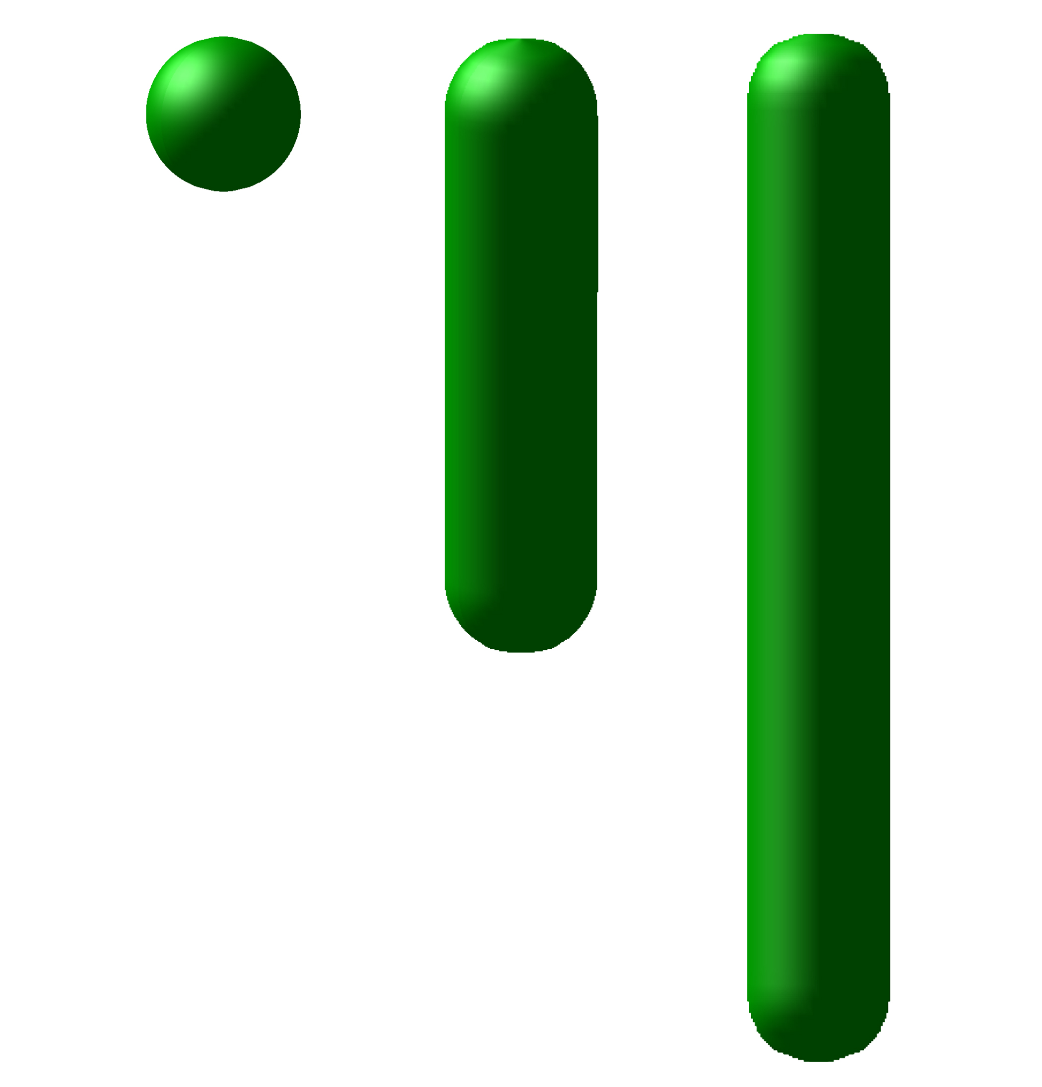
Figure 1: Plot of the spherocylindrical capsule with the length-to-radius ratio equal to $0$, $2\pi$ and $4\pi$ in actual scales.

In this section, we solve the tangential Schrödinger equation (4) on the surface of the so-called spherocylindrical capsule. A spherocylindrical capsule is a compact surface consisting of a circular finite cylinder of radius $R$ and length $L$ which is closed on both ends by a hemisphere of radius $R$ as is depicted in Fig. 1. To parametrize the entire surface homogeneously, we introduce the map

$$\mathbf{f}\left(z,\varphi\right)=z\hat{k}+a\left(z\right)\left(\hat{\imath}\cos\varphi+\hat{\jmath}\sin\varphi\right),$$ (19)

in which $-R-\frac{L}{2}<z<\frac{L}{2}+R$ is the axis of the capsule and $0<\varphi<2\pi$ is the usual azimuthal angle. Furthermore, $a\left(z\right)$ is the variable radius of the cross-section of the capsule at any given $z$ expressed by

$$a\left(z\right)=\left\{\begin{array}[]{lr}\sqrt{R^{2}-\left(z+\frac{L}{2}\right)^{2}}&-R-\frac{L}{2}\leq z\leq-\frac{L}{2}\\ R&-\frac{L}{2}\leq z\leq\frac{L}{2}\\ \sqrt{R^{2}-\left(z-\frac{L}{2}\right)^{2}}&\frac{L}{2}\leq z\leq\frac{L}{2}+R\end{array}\right.,$$ (20)

and $\hat{\imath},\hat{\jmath}$ and $\hat{k}$ are the usual constant unit vectors. Having the surface patch defined in (19) and (20), we proceed to obtain the first fundamental form which is obtained to be

$$h_{ab}=\left(\begin{array}[]{cc}\mathbf{f}_{,z}.\mathbf{f}_{,z}&\mathbf{f}_{,z}.\mathbf{f}_{,\varphi}\\ \mathbf{f}_{,\varphi}.\mathbf{f}_{,z}&\mathbf{f}_{,\varphi}.\mathbf{f}_{,\varphi}\end{array}\right)=\left(\begin{array}[]{cc}1+a^{\prime}\left(z\right)^{2}&0\\ 0&a\left(z\right)^{2}\end{array}\right),$$ (21)

where a prime stands for the derivative with respect to $z.$ Moreover, we introduce the normal unit vector to the surface (outward direction)

$$\hat{N}=-\frac{\mathbf{f}_{,z}\times\mathbf{f}_{,\varphi}}{\left\|\mathbf{f}_{,z}\times\mathbf{f}_{,\varphi}\right\|}=\frac{\hat{\imath}\cos\varphi+\hat{\jmath}\sin\varphi-a^{\prime}\hat{k}}{\sqrt{1+a^{\prime}\left(z\right)^{2}}},$$ (22)

upon which we calculate the second fundamental form i.e.,

$$\kappa_{ab}=\left(\begin{array}[]{cc}\mathbf{f}_{,zz}.\hat{N}&\mathbf{f}_{,z\varphi}.\hat{N}\\ \mathbf{f}_{,\varphi z}.\hat{N}&\mathbf{f}_{,\varphi\varphi}.\hat{N}\end{array}\right)=\frac{1}{\sqrt{1+a^{\prime}\left(z\right)^{2}}}\left(\begin{array}[]{cc}a^{\prime\prime}&0\\ 0&-a\end{array}\right).$$ (23)

Finally, we calculate the mixed extrinsic curvature tensor

$$\kappa_{a}^{b}=h^{bc}\kappa_{ac}=\frac{1}{\sqrt{1+a^{\prime}\left(z\right)^{2}}}\left(\begin{array}[]{cc}\frac{a^{\prime\prime}}{1+a^{\prime}\left(z\right)^{2}}&0\\ 0&-\frac{1}{a}\end{array}\right),$$ (24)

from which we calculate the total and Gaussian curvatures i.e.,

$$K=\text{Tr}\left(\kappa_{a}^{b}\right)=\frac{1}{\sqrt{1+a^{\prime}\left(z\right)^{2}}}\left(\frac{a^{\prime\prime}}{1+a^{\prime}\left(z\right)^{2}}-\frac{1}{a}\right),$$ (25)

and

$$K_{G}=\det\left(\kappa_{a}^{b}\right)=\frac{-a^{\prime\prime}}{a\left(1+a^{\prime}\left(z\right)^{2}\right)^{2}}.$$ (26)

Having $K$ and $K_{G}$ calculated in (25) and (26), the geometric potential (5) becomes

$$V_{G}\left(z,\varphi\right)=\left\{\begin{array}[]{lr}0&-R-\frac{L}{2}\leq z\leq-\frac{L}{2}\\ -\frac{\hbar^{2}}{8R^{2}M}&-\frac{L}{2}\leq z\leq\frac{L}{2}\\ 0&\frac{L}{2}\leq z\leq\frac{L}{2}+R\end{array}\right.,$$ (27)

as was expected. Next, we introduce the tangential/local wave function in the form

$$\psi^{\left(T\right)}\left(z,\varphi\right)=e^{im\varphi}Y\left(z\right),$$ (28)

such that (4) with zero-tangential/local energy becomes

$$-\frac{\hbar^{2}}{2M}\frac{1}{\sqrt{1+a^{\prime}\left(z\right)^{2}}}\frac{d}{dz}\left(\frac{1}{\sqrt{1+a^{\prime}\left(z\right)^{2}}}\frac{d}{dz}\right)Y\left(z\right)+\frac{\hbar^{2}m^{2}}{2Ma\left(z\right)^{2}}Y\left(z\right)+V_{G}Y\left(z\right)=0,$$ (29)

in which $m$ is an integer number due to the azimuthal symmetry of the capsule. Knowing that on the surface

$$\sqrt{1+a^{\prime}\left(z\right)^{2}}=\frac{R}{a\left(z\right)},$$ (30)

the explicit form of (29) is given by

$$-\frac{\hbar^{2}}{2M}\frac{a\left(z\right)}{R}\frac{d}{dz}\left(\frac{a\left(z\right)}{R}\frac{d}{dz}\right)Y\left(z\right)+\frac{\hbar^{2}m^{2}}{2Ma\left(z\right)^{2}}Y\left(z\right)+V_{G}Y\left(z\right)=0.$$ (31)

In terms of different regions on the capsule, (31) reads

$$\left\{\begin{array}[]{lr}-\frac{\hbar^{2}}{2M}\frac{\sqrt{R^{2}-\left(z+\frac{L}{2}\right)^{2}}}{R}\frac{d}{dz}\left(\frac{\sqrt{R^{2}-\left(z+\frac{L}{2}\right)^{2}}}{R}\frac{d}{dz}\right)Y_{I}\left(z\right)+\frac{\hbar^{2}m^{2}}{2M\left(R^{2}-\left(z+\frac{L}{2}\right)^{2}\right)}Y_{I}\left(z\right)=0&-R-\frac{L}{2}\leq z\leq-\frac{L}{2}\\ -\frac{\hbar^{2}}{2M}\frac{d^{2}}{dz^{2}}Y_{II}\left(z\right)+\frac{\hbar^{2}}{2MR^{2}}\left(m^{2}-\frac{1}{4}\right)Y_{II}\left(z\right)=0&-\frac{L}{2}\leq z\leq\frac{L}{2}\\ -\frac{\hbar^{2}}{2M}\frac{\sqrt{R^{2}-\left(z-\frac{L}{2}\right)^{2}}}{R}\frac{d}{dz}\left(\frac{\sqrt{R^{2}-\left(z-\frac{L}{2}\right)^{2}}}{R}\frac{d}{dz}\right)Y_{III}\left(z\right)+\frac{\hbar^{2}m^{2}}{2M\left(R^{2}-\left(z-\frac{L}{2}\right)^{2}\right)}Y_{III}\left(z\right)=0&\frac{L}{2}\leq z\leq\frac{L}{2}+R\end{array}\right.,$$ (32)

where we used the subindices I, II, and III for the left, middle, and right sides of the capsule. By introducing $z=-\frac{L}{2}+qR$ and $L=\lambda R$ in which $q$ is the new variable and $\lambda=\frac{L}{R}$ being the length-to-radius ratio, the first equation in (32) simplifies to

$$-\sqrt{1-q^{2}}\frac{d}{dq}\left(\sqrt{1-q^{2}}\frac{d}{dq}\right)Y_{I}\left(q\right)+\frac{m^{2}}{1-q^{2}}Y_{I}\left(q\right)=0,$$ (33)

which is the same as Eq. (14) after considering $\cos\theta=q$. With $-R-\frac{L}{2}\leq z\leq-\frac{L}{2}$, we find $-1\leq q\leq 0$ and the only finite solution of (33) in this interval corresponds to $m=0$ and

$$Y_{I}\left(q\right)=C_{I},$$ (34)

in which $C_{I}$ is an integration constant. Similarly in the third region, we introduce $z=\frac{L}{2}+qR$ and $L=\lambda R$ to get

$$-\sqrt{1-q^{2}}\frac{d}{dz}\left(\sqrt{1-q^{2}}\frac{d}{dz}\right)Y_{III}\left(z\right)+\frac{m^{2}}{1-q^{2}}Y_{III}\left(z\right)=0,$$ (35)

such that $0\leq q\leq 1$. With the same reason here also $m=0$ and the only solution being finite in the domain of $q$ is

$$Y_{III}\left(q\right)=C_{III}.$$ (36)

Finally, the tangential Schrödinger equation in the middle region after introducing $m=0$ due to the continuity condition of the wave function becomes

$$\frac{d^{2}}{dz^{2}}Y_{II}\left(z\right)+\frac{1}{4R^{2}}Y_{II}\left(z\right)=0,$$ (37)

which admits a solution in the form of

$$Y_{II}\left(z\right)=A\cos\left(\frac{z}{2R}\right)+B\sin\left(\frac{z}{2R}\right),$$ (38)

in which $A$ and $B$ are two integration constants. After we obtained the solutions on all regions we have to apply the boundary conditions. In particular since we set $m=0$ the azimuthal part of the wave function is trivially continuous. The non-azimuthal part of the wave function i.e., $Y\left(z\right)$ and its first derivative i.e., $Y^{\prime}\left(z\right)$ have to be continuous everywhere on the surface of the capsule. In particular we apply these conditions at $z=-\frac{L}{2}$ and $z=\frac{L}{2}.$ The wave function and its first derivatives are given by

$$Y\left(z\right)=\left\{\begin{array}[]{lr}C_{I}&-R-\frac{L}{2}\leq z\leq-\frac{L}{2}\\ A\cos\left(\frac{z}{2R}\right)+B\sin\left(\frac{z}{2R}\right)&-\frac{L}{2}\leq z\leq\frac{L}{2}\\ C_{III}&\frac{L}{2}\leq z\leq\frac{L}{2}+R\end{array}\right.,$$ (39)

and

$$Y^{\prime}\left(z\right)=\left\{\begin{array}[]{lr}0&-R-\frac{L}{2}\leq z\leq-\frac{L}{2}\\ -\frac{A}{2R}\sin\left(\frac{z}{2R}\right)+\frac{B}{2R}\cos\left(\frac{z}{2R}\right)&-\frac{L}{2}\leq z\leq\frac{L}{2}\\ 0&\frac{L}{2}\leq z\leq\frac{L}{2}+R\end{array}\right.,$$ (40)

respectively. The continuity of the wave function and its derivative at $z=-\frac{L}{2}$ and $z=\frac{L}{2}$ yield

$$\text{the boundary conditions}\Longrightarrow\left\{\begin{array}[]{l}A\cos\left(\frac{L}{4R}\right)-B\sin\left(\frac{L}{4R}\right)=C_{I}\\ A\cos\left(\frac{L}{4R}\right)+B\sin\left(\frac{L}{4R}\right)=C_{III}\\ A\sin\left(\frac{L}{4R}\right)+B\cos\left(\frac{L}{42R}\right)=0\\ -A\sin\left(\frac{L}{4R}\right)+B\cos\left(\frac{L}{4R}\right)=0\end{array}\right..$$ (41)

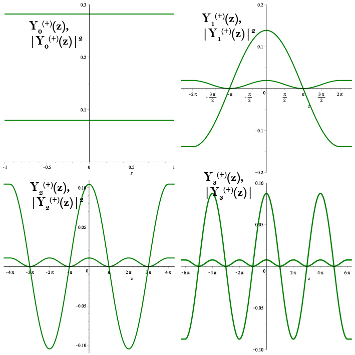
Figure 2: Plots of the wavefunctions $Y_{k}^{\left(+\right)}$ and $\left|Y_{k}^{\left(+\right)}\right|^{2}$ in terms of the axial variable $z$ for the first four even states i.e., $k=0,1,2$ and $4$ corresponding to the length-to-radius ration $\lambda_{k}^{\left(+\right)}=\frac{L_{k}^{\left(+\right)}}{R}=4k\pi.$ The upper panel left plot corresponds to the spherical capsule where the probability density is uniform over the surface of the sphere. This uniform probability can be seen in the other three graphs only on the hemispheres in the left and the right of the graph. The probability on the cylindrical part of the capsule, however, is not uniform and instead is periodic.

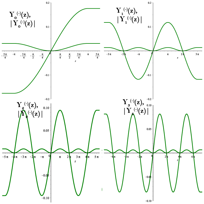
Figure 3: Plots of the wavefunctions $Y_{k}^{\left(-\right)}$ and $\left|Y_{k}^{\left(-\right)}\right|^{2}$ in terms of the axial variable $z$ for the first four odd states i.e., $k=0,1,2$ and $3$ corresponding to the length-to-radius ration $\lambda_{k}^{\left(-\right)}=\frac{L_{k}^{\left(-\right)}}{R}=2\left(2k+1\right)\pi.$ Similar to the even states, here also the probability density on the two hemispheres is uniform and on the cylindrical part of the capsule is periodic.

The last two equations admit nontrivial solutions for $A$ and $B$ if and only if

$$\sin\left(\frac{L}{4R}\right)\cos\left(\frac{L}{4R}\right)=0.$$ (42)

Hence, while with $\cos\left(\frac{L}{2R}\right)=0$ one gets $A=0$ and $B\neq 0$, with $\sin\left(\frac{L}{2R}\right)=0$ it yields $B=0$ and $A\neq 0.$ For the former case the first two equations imply $C_{III}=-C_{I}=B\sin\left(\frac{L}{2R}\right)$ and therefore the solution becomes

$$Y^{\left(-\right)}\left(z\right)=\left\{\begin{array}[]{lr}-B\sin\left(\frac{L}{4R}\right)&-R-\frac{L}{2}\leq z\leq-\frac{L}{2}\\ B\sin\left(\frac{z}{4R}\right)&-\frac{L}{2}\leq z\leq\frac{L}{2}\\ B\sin\left(\frac{z}{4R}\right)&\frac{L}{2}\leq z\leq\frac{L}{2}+R\end{array}\right.\text{ with }\frac{L}{4R}=\left(k+\frac{1}{2}\right)\pi.\text{ }$$ (43)

On the other hand for the latter case, the first two equations yield $C_{III}=C_{I}=A\cos\left(\frac{L}{4R}\right)$ and the wave function reads

$$Y^{\left(+\right)}\left(z\right)=\left\{\begin{array}[]{lr}A\cos\left(\frac{L}{4R}\right)&-R-\frac{L}{2}\leq z\leq-\frac{L}{2}\\ A\cos\left(\frac{z}{4R}\right)&-\frac{L}{2}\leq z\leq\frac{L}{2}\\ A\cos\left(\frac{L}{4R}\right)&\frac{L}{2}\leq z\leq\frac{L}{2}+R\end{array}\right.\text{ with }\frac{L}{4R}=k\pi.$$ (44)

Herein, the superindices $\pm$ stand for the even and odd solution and $k=0,1,2,3,...$. To normalize the wave function, we write

$$\int_{0}^{2\pi}\int_{-R-\frac{L}{2}}^{R+\frac{L}{2}}\left|Y^{\left(\pm\right)}\left(z\right)\right|^{2}\sqrt{h}dzd\varphi=1,$$ (45)

in which

$$h=\det h_{ab}=\left(1+a^{\prime}\left(z\right)^{2}\right)a\left(z\right)^{2}=R^{2},$$ (46)

in all regions. Explicitly (45) for the even solution reads

$$2\pi R\left|A\right|^{2}\left(\int_{-R-\frac{L}{2}}^{-\frac{L}{2}}dz+\int_{-\frac{L}{2}}^{+\frac{L}{2}}\cos^{2}\left(\frac{z}{2R}\right)dz+\int_{\frac{L}{2}}^{\frac{L}{2}+R}dz\right)=1,$$ (47)

in which we used $\cos\left(\frac{L}{4R}\right)=\cos\left(k\pi\right)=\left(-1\right)^{k}.$ Hence, we obtain

$$\left|A\right|^{2}=\frac{1}{2\pi R\left(2R+\frac{L}{2}\right)}=\frac{1}{4\pi R^{2}\left(1+k\pi\right)}.$$ (48)

A similar calculation for the odd wave function yields

$$\left|B\right|^{2}=\frac{1}{4\pi R^{2}\left(1+\left(k+\frac{1}{2}\right)\pi\right)}.$$ (49)

Finally, the normalized wave function is expressed by

$$\psi_{n,k}^{\left(+\right)}\left(z,\varphi,w,t\right)=\sqrt{\frac{\varepsilon}{8\pi R^{2}\left(1+k\pi\right)}}\left\{\begin{array}[]{lr}\left(-1\right)^{k}\sin\left(\frac{n\pi}{\varepsilon}w\right)e^{-iE_{n}t/\hbar}&-R-\frac{L}{2}\leq z\leq-\frac{L}{2}\\ \cos\left(\frac{z}{2R}\right)\sin\left(\frac{n\pi}{\varepsilon}w\right)e^{-iE_{n}t/\hbar}&-\frac{L}{2}\leq z\leq\frac{L}{2}\\ \left(-1\right)^{k}\sin\left(\frac{n\pi}{\varepsilon}w\right)e^{-iE_{n}t/\hbar}&\frac{L}{2}\leq z\leq\frac{L}{2}+R\end{array}\right.,$$ (50)

and

$$\psi_{n,k}^{\left(-\right)}\left(z,\varphi,w,t\right)=\sqrt{\frac{\varepsilon}{8\pi R^{2}\left(1+\left(k+\frac{1}{2}\right)\pi\right)}}\left\{\begin{array}[]{lr}\left(-1\right)^{k+1}\sin\left(\frac{n\pi}{\varepsilon}w\right)e^{-iE_{n}t/\hbar}&-R-\frac{L}{2}\leq z\leq-\frac{L}{2}\\ \sin\left(\frac{z}{2R}\right)\sin\left(\frac{n\pi}{\varepsilon}w\right)e^{-iE_{n}t/\hbar}&-\frac{L}{2}\leq z\leq\frac{L}{2}\\ \left(-1\right)^{k}\sin\left(\frac{n\pi}{\varepsilon}w\right)e^{-iE_{n}t/\hbar}&\frac{L}{2}\leq z\leq\frac{L}{2}+R\end{array}\right..$$ (51)

We note that, in both cases, the total energy is equal to the normal/global energy i.e., $E_{n}=E_{n}^{\left(N\right)}=\frac{n^{2}\pi^{2}\hbar^{2}}{2M\varepsilon^{2}},$ $n=1,2,3,...$ because the local energy was set to zero. Furthermore, the wave functions (50) and (51) both exist only if and only if the length-to-radius ratio $\lambda_{k}^{\left(\pm\right)}=\frac{L}{R}$ is quantized. The first quantized length is $\lambda_{0}^{\left(+\right)}=0$ which corresponds to the spherical shell. In other words, the capsule is a sphere that has been studied separately in the previous section. The second, third, and fourth quantized length-to-radius ratio correspond to $\lambda_{0}^{\left(-\right)}=\pi$, $\lambda_{1}^{\left(+\right)}=2\pi$ and $\lambda_{1}^{\left(-\right)}=3\pi$, respectively. In Fig. 2 and 3, we plot the tangential even/odd wave functions i.e., $Y_{k}^{\left(\pm\right)}\left(z\right)$ and the corresponding probability densities i.e., $\left|Y_{k}^{\left(\pm\right)}\left(z\right)\right|^{2}$ in terms of $z$ for the first, second, third, and fourth quantized length-to-radius ratio for each parity i.e., even and odd.

Our calculations show that with the $\frac{L}{R}=\lambda_{k}^{\left(\pm\right)}$ the wave function of the particle with zero local energy makes constructive interference with itself such that the stationary wave function is nonzero and normalizable. On the other hand when $\frac{L}{R}\neq\lambda_{k}^{\left(\pm\right)}$ the wave function makes a kind of destructive interference with itself such that its wave function eventually vanishes. Such particles cannot exist with zero local energy and must jump on any other possible energy level corresponding to a wave function that satisfies all boundary conditions. We assume hypothetically that there exists a mechanism upon which we can measure the local energy of a quantum particle confined on a spherocylindrical capsule. Since the zero energy corresponds to a quantized $\frac{L}{R}$, a nonzero wave function for such a particle implies the size of the capsule and vice versa. Therefore, we may have created an indirect method to measure the size of nanotubes as well as the energy of the quantum particles on those nanotubes.

V Conclusion

In this research, we studied a spinless nonrelativistic quantum particle on a spherocylindrical capsule. Employing Costa’s formalism Costa , we solved the corresponding Schrödinger equation by separating it into a normal/global component multiplied by a tangent/local component. Assuming a homogeneous and very thin surface, the normal or global component simply became a one-dimensional infinite well problem with exact eigenfunctions and eigenenergies. The tangent or local component, however, needed to be treated in three different regions on the surface of the capsule. After we assumed the tangent or local energy of the particle to be zero, we were able to solve the 2-dimensional Schrödinger equation on the three different regions on the surface. Moreover, upon imposing the boundary conditions consisting of the continuity of the wave function as well as its first derivative, we obtained a relation between the geometric structure of the capsule and the existence of a nonzero wave function. In summary, we can state the results as follows: While a spinless nonrelativistic particle with energy $E_{n}=\frac{n^{2}\pi^{2}\hbar^{2}}{2M\varepsilon^{2}},$ $n=1,2,3,...$ can live on a spherical surface of radius $R$ and thickness $\varepsilon$ with a uniform probability distribution everywhere on the surface, the same particle cannot survive on the surface of a spherocylindrical capsule of the same radius $R$ for the hemispheres, length $L$ for the cylindrical body and thickness $\varepsilon$ unless $\frac{L}{R}$ is equal to an even multiplication of $\pi$. Precisely, we found $\frac{L}{R}=2\left(2k+1\right)\pi,4k\pi$ where $k=0,1,2,...$. Physically it can be understood in the context of the constructive or destructive interference of the wave function of the particle with itself for $\frac{L}{R}=2\left(2k+1\right)\pi,4k\pi$ or $\frac{L}{R}\neq 2\left(2k+1\right)\pi,4k\pi,$ respectively.  On one hand, the mechanism of having a non-zero wave function with a given energy on the surface of the capsule may be used to measure precisely the size of such nanotubes. On the other hand upon knowing the size of the capsule and a nonzero wave function on the surface hypothetically one may find the energy of such a particle.

References

• (1) F. Santos, S. Fumeron, B. Berche, F. Moraes, Nanotechnology 27, 135302 (2016).
• (2) A. Marchi, S. Reggiani, M. Rudan, A. Bertoni, Phys. Rev. B 72, 035403 (2005).
• (3) R. Cheng, Y.-L. Wang, H.-X. Gao, H. Zhao, J.-Q, Wang, and H.-S. Zong, J. Phys.: Condens. Matter 32, 025504 (2020).
• (4) M. Katsnelson, 2012, Graphene: Carbonin Two Dimensions (Cambridge: Cambridge University Press).
• (5) A. H. Castro Neto, F. Guinea, N. M. R. Peres, K. S. Novoselov, and A. K. Geim, Rev. Mod. Phys. 81, 109 (2009).
• (6) A. K. Geim, and K. S. Novoselov, Nature Mater 6, 183 (2007).
• (7) A. de J. Espinosa-Champo, G. G. Naumis, and P. C.-Villarreal, Phys. Rev. B 110, 035421 (2024).
• (8) S. Berber, Y. K. Kwon and D. Tomanek, Phys. Rev. Lett. 84, 4613 (2000).
• (9) L. Wei, P. K. Kuo, R. L. Thomas, T. R. Anthony, and W. F. Banholzer, Phys. Rev. Lett. 70, 3764 (1993).
• (10) S. Iijima, Nature (London) 354, 56 (1991).
• (11) A. Carvalho, M. Wang, X. Zhu, A. S. Rodin, H. Su, and A. H. Castro Neto, Nat. Rev. Mater. 1, 11 (2016).
• (12) B. S. D. Witt, Rev. Modern Phys. 29, 377 (1957).
• (13) H. Jensen, H. Koppe, Ann. Phys. 63, 586 (1971).
• (14) R. C. T. de Costa, Phys. Rev. A 23, 1982 (1981).
• (15) R.C.T. da Costa, Phys. Rev. A 25, 2893 (1982).
• (16) G. Ferrari, G. Cuoghi, Phys. Rev. Lett. 100, 230403 (2008).
• (17) G-H Liang, and M-Y. Lai, Phys. Rev. A 107, 022213 (2023).
• (18) L. Meschede, B. Schwager, D. Schulz, and J. Berakdar, Phys. Rev. A 107, 062806 (2023).
• (19) L-L. Ye, C.-D. Han, L. Huang, and Y-C. Lai, Phys. Rev. A 106, 022207 (2022).
• (20) J. E. G. Silva, J. Furtado, and A. C. A. Ramos, Eur. Phys. J. B 94, 127 (2021).
• (21) J. Gravesen, M. Willatzen, and L. C. L. Yan Voon, J. Math. Phys. 46, 012107 (2005).
• (22) A. G. M. Schmidt and M. E. Pereira, Phys. Lett. A 517, 129674 (2024).
• (23) A. G. M. Schmidt, Braz. J. Phys. 50, 419 (2020).
• (24) A. G. M. Schmidt, M.E. Pereira, J. Math. Phys. 64, 042101 (2023).
• (25) J. E. G. Silva, J. Furtado, A. C. A. Ramos, Eur. Phys. J. B 94, 127 (2021).
• (26) T. F. de Souza, A. C. A. Ramos, R. N. Costa Filho, J. Furtado, Phys. Rev. B 106, 165426 (2022).
• (27) Z. Q. Yang, X. Y. Zhou, Z. Li, W. K. Du, and Q. H. Liu, Phys. Lett. A 384, 126604 (2020).
• (28) J. E. G. Silva, J. Furtado, T. M. Santiago, A. C.A. Ramos, D. R. da Costa, Phys. Lett. A 384, 126458 (2020).
• (29) G. C-Acosta, H. H-Hernandez, and J. R-Rascon, Ann. Phys. 467, 169695 (2024).
• (30) S. H. Mazharimousavi, Phys. Scr. 96, 125245 (2021).