Local Exchange-Correlation Potentials by Density Inversion in Solids
Abstract
Following Hollins et al. [J. Phys.: Condens. Matter 29, 04LT01 (2017)], we invert the electronic ground state densities for various semiconducting and insulating solids calculated using several density functional approximations within the generalised Kohn-Sham (GKS) scheme, Hartree-Fock (HF) theory and the LDA+ method, and benchmark against standard (semi-)local functionals. The band structures from the resulting local exchange-correlation (LXC) Kohn-Sham potential for these densities are then compared with the band structures of the original GKS method. We find the LXC potential obtained from the HF density systematically predicts band gaps in good agreement with experiment, even in strongly correlated transition metal monoxides (TMOs). Furthermore, we find that the HSE06 and PBE0 hybrid functionals yield similar densities and LXC potentials, and in weakly correlated systems, these potentials are similar to PBE. For LDA+ densities, the LXC potential effectively reverses the flattening of bands caused by over-localisation by a large Hubbard- value, while for meta-GGAs, we find only small differences between the GKS and LXC results demonstrating that the non-locality of meta-GGAs is weak.
I Introduction
Density functional theory (DFT) has enjoyed considerable success as a framework for modelling and obtaining theoretical insight into the behaviour of materials at a relatively low computational cost. Within the Kohn-Sham(KS)[1] formulation, this is realised through a fictitious auxiliary non-interacting system of electrons constructed to yield an identical ground state density to the interacting system. Although a formally exact theory in principle, in practice the exchange-correlation (XC) contribution to the total energy density functional needs to be approximated. Consequently, the resulting XC potential of any density functional approximation (DFA),
| (1) |
will differ from the corresponding of the exact theory.
The solution to the standard KS problem involves finding the ground state density and in an iterative fashion beginning with a trial density and calculating , solving the KS equations and updating the density, repeating the process until self-consistency has been achieved. The development and refinement of approximations for remains challenging, not least because the exact or are not experimentally observable and thus, one lacks a benchmark to which one can compare.
Although previous work using many-body perturbation theory[2, 3, 4, 5, 6] has been carried out in simple semiconductors to gain some insight and study the behaviour of the exact , an alternative, albeit indirect approach to construct the exact is through the inverse KS or density inversion problem. Because of the one-to-one correspondence between the KS potential and established by the Hohenberg-Kohn theorems[7, 8], one can seek the local exchange-correlation (LXC) potential , that will adopt a target density as its ground state. If the target density is obtained by sufficiently accurate means, for instance from quantum Monte Carlo (QMC) calculations[9] such that it may be regarded as “exact”, the technique can be used to study the corresponding “exact” KS potential.
Moreover, density inversion can also be used to study and analyse the quality of approximate densities and their corresponding local XC potentials. Considerable work has been carried out in recent years in understanding errors within DFT calculations[10, 11, 12, 13, 14, 15, 16, 17, 18, 19, 20, 21]. According to an insightful analysis by Burke and coworkers, the error in the approximate total energy of a DFT calculation may be partitioned into the “functional error” and the so-called “density-driven error”[22, 23, 24, 25, 26], the significance of which can be investigated using density inversion[27]. The former is the most common and refers to the quality of the approximation for the XC energy density functional for the exact density. The latter arises in “abnormal” systems [22], where the density is particularly sensitive to changes in , giving rise to large errors in the density, which are only further exacerbated by the self-consistent cycle. In such instances, the use of the Hartree-Fock (HF) density in a non-self-consistent manner can give improved total energies such as in water clusters[28, 29, 30, 31, 32].
Finally, density inversion is closely connected to the optimised effective potential (OEP) method[33, 34], notably the direct OEP method developed by Wu and Yang[35] which can be adapted to invert densities[36] with a similar approach by Görling[37, 38]. In a wider sense, OEP is of interest for the application of implicit density functionals, which can potentially offer greater accuracy through the satisfaction of a greater number of exact constraints[39, 40]. Due to numerical issues such as those caused by the use of finite basis sets[41, 42], the difficulty in the calculation of the full OEP in a computationally efficient and robust manner[43, 44] has limited the wider adoption of the OEP method.
Despite the appeal of density inversion as a benchmarking and functional development tool for the aforementioned reasons, the inversion of the density remains a somewhat formidable task due to the sensitivity of the potential to errors in the density[45, 46] and thus the problem remains an active area of research with various inversion schemes proposed [47, 48, 37, 49, 50, 51, 36, 52, 53, 54, 55, 56, 57, 58, 59, 60, 61, 62, 63]. In this work, we use the scheme developed by Hollins et al.[64] to compare the LXC potential obtained via densities produced by approximations with increasing degrees of non-locality in their single-particle Hamiltonians. We then compare the calculated band structures from the LXC potential and from the self-consistent non-local potential as well as their total energy differences, when the total energy functional is evaluated using the self-consistent orbitals and the orbitals obtained via the LXC potential.
This paper is structured as follows. In section II, we overview our method used to invert densities to find the LXC potential and its implementation in a plane-wave pseudopotential code. Section III describes the various computational parameters we have used and also introduces the systems used in this study. In section IV, we present computed band structures from the LXC potentials and from self-consistent KS and generalised Kohn-Sham (GKS) schemes. Section IV.1 presents the inversion of local/semi-local LDA and PBE densities to quantify the degree of numerical error in the inversion algorithm. We then discuss the inversion of HF densities and hybrid functionals in sections IV.2 and IV.3 where we also discuss the difference in total energy when a given DFA is evaluated using self-consistent GKS orbitals and the LXC orbitals as a quantitative indicator of the non-locality. Results from the inversion of LDA+ densities in transition metal monoxides (TMOs) are presented in section IV.4. We then discuss the inversion of densities from a meta-GGA functional (rSCAN) when treated in a GKS scheme. Finally, we discuss the magnitude of the exchange-correlation derivative discontinuity for the LXC potential in section V before we draw conclusions and discuss plans for future work in section VI.
II Theory
We follow the density inversion method of references [64, 56, 57]. We consider a non-interacting system of particles moving within a local effective potential with a ground state density . The full Hamiltonian of this non-interacting system can be expressed as a sum of single-particle Hamiltonians with single-particle energies ,
| (2) |
The goal is to invert a “target” density, obtained from some electronic structure or quantum chemical method to find the local effective potential such that has a ground state density equal to the target density, .
Consider the Coulomb energy associated with the difference in the target density and the ground state density of the local potential ,
| (3) |
When the two densities are equal, ,
and thus the KS potential is found and the density inversion problem solved.
The KS potential is customarily partitioned into an external , Hartree and exchange-correlation potentials
| (4) |
In this work, we will refer to the exchange-correlation of the KS potential obtained via density inversion of a target density as the local exchange-correlation (LXC) potential (emphasising that it is a local multiplicative potential). Since , it is thus possible to invert a given target density via minimisation of . A change in the potential, with causes a change in
| (5) |
Applying the chain rule and noting the change in the density is related to the density-density response function
| (6) |
We can thus express the change in the Hartree energy given in Eq. (5)
| (7) |
We now choose for Eq. (7)
| (8) |
as used, for instance, in the inversion methods of Zhao, Morrison and Parr[50] and Görling[38]. Using this form for leads to faster convergence compared to simply using the density difference, , particularly in regions of low density[64]. Moreover, the form of in Eq. (8) ensures that is minimised for a sufficiently small value of as because the response function is a negative semi-definite operator. For these reasons, can be regarded as an effective gradient of .
.
In a steepest descent algorithm, see Fig. 1, the potential is thus updated by taking a step in the direction of the effective gradient
| (9) |
where is the step size calculated using a line search, as discussed further in section II.2. The density adopted by the local potential is then updated by solving the KS equations
| (10) |
to find the orbitals associated with the updated local effective potential . We then calculate the Hartree energy , see Eq. (3) of the density difference . This iterative procedure is repeated until the target density and the density of the local effective potential, , are equal within a small tolerance such that is effectively zero. In practice, we use a more efficient conjugate gradient[65] algorithm.
As an aside, we note the inverse KS problem is strictly defined for densities which are ground state -representable, that is to say, ground state densities of local multiplicative potentials .
II.1 Orbitals of the Non-Interacting System and Total Energies
The orbitals that yield the density of the non-interacting system bound by a local potential can be regarded as density optimal[66] in the sense that they yield an identical density to the target density . Suppose that the target density is obtained via a DFA which has an explicit dependence on orbitals but not on the density . This DFA can be regarded as an implicit functional of the density since the KS orbitals are determined by the KS potential which in turn depends on the density. These DFAs can always be treated within a standard KS scheme using single-particle equations that contain a local, multiplicative potential via the OEP method[40, 67]. Alternatively, one can instead consider them in a generalised Kohn-Sham (GKS) scheme with non-local single-particle equations.
The KS orbitals obtained from the inversion of the density are not energy optimal as they do not fully minimise the total energy functional of the DFA, , and in the case of such DFAs, the GKS scheme yields a lower energy. Equivalently, the effective potential , and by extension the LXC potential obtained for this DFA density , is not the minimising potential of ; instead the minimising potential is non-local and in general, . Therefore, if one evaluates in a non-self-consistent manner using the orbitals from the inversion, then
| (11) |
where are the self-consistent set of GKS orbitals associated with the minimising non-local GKS potential. The magnitude of the energy difference in Eq. (11) will depend on the degree of non-locality in the Hamiltonian .
In the case of HF densities, the potential obtained via inversion of the HF density is the local Fock exchange (LFX) potential [63, 58, 59, 60, 64, 68, 56, 57], . The inversion of HF densities yields a local potential similar to the exact-exchange-only (EXX) potential (without correlation or exchange-only OEP (xOEP)), particularly in weakly correlated systems[54, 61, 62, 69, 70, 71, 59, 60, 72, 43, 64, 73]. This is due to the fact that the xOEP potential and LFX potential minimise physically equivalent energy differences[64, 8].
II.2 Implementation in a Plane-Wave Code
The algorithm to carry out the inversion of the density to find the LXC potential has been implemented in the plane-wave DFT code CASTEP[74]. As is usual with plane-wave implementations, the density, orbitals and potentials are represented on rectilinear grids[75]. The KS orbitals are described within a spherical region of reciprocal space with a radius equal to the cutoff wave vector , while the density and potential are non-zero in a region of . The density is inverted through minimisation of the Coloumb energy difference , see Eq. (3) and is performed in real space to enable direct variation of the potential, see Eq. (8).
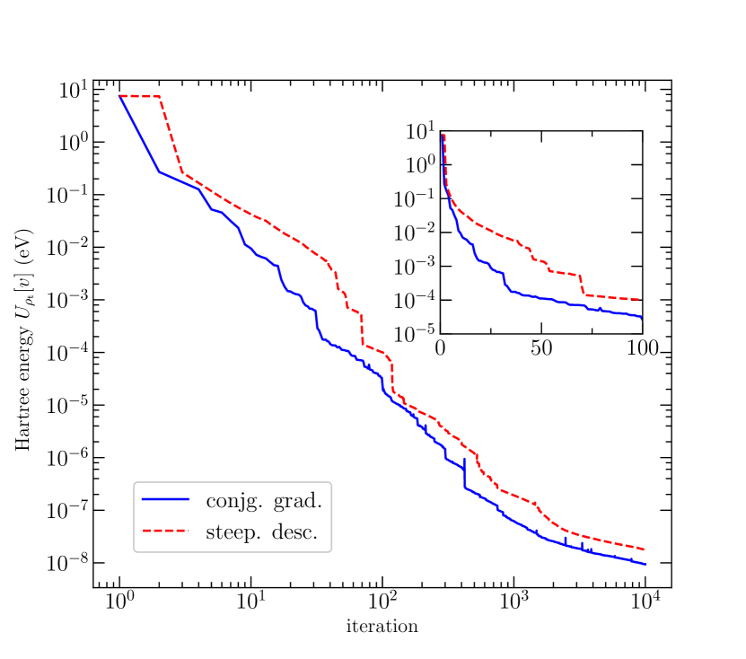
A Fletcher-Reeves-based conjugate gradient algorithm[65] is the algorithm of choice for the minimisation and is used to compute the search direction (in steepest descent this is simply Eq. (8)). The potential is then corrected along this search direction multiplied by a prefactor , whose optimal value is determined via a line search that minimises using a parabolic three-step fit. Fig. 2 compares the convergence of for the inversion of the HF density of silicon for steepest descent and conjugate gradient algorithms with the initial LXC potential set to the local density approximation (LDA) potential generated by the HF density. Although the steepest descent algorithm exhibits a similarly shaped decrease in to conjugate gradient, the rate of convergence starts to fall off rapidly after around 20 iterations only reaching a value of after around 100 iterations, whereas the conjugate gradient algorithm reaches a value of . In both cases, the effective gradient term, see Eq. (8), tends to zero as expected from a variational method.
For our actual calculations, the differences in were monitored over a window of iterations (we find works well), denoted . The minimisation procedure was repeated until the difference between the largest and smallest values of within the window is smaller than the threshold value of , that is to say,
| (12) |
We find that was sufficiently small to ensure that the calculation was well converged. This ensured that the algorithm did not terminate prematurely due to a plateau in the energy landscape.
III Computational Details
For all calculations presented here, the plane-wave cutoff energy and Monkhorst-Pack[76] grid for Brillouin zone sampling were selected such that the self-consistent total energy was converged to less than . The inversion algorithm was considered converged when the difference of the Hartree energy within a window of three iterations was less than eV/atom.
With regard to the choice of pseudopotentials, we used norm-conserving pseudopotentials (NCPs) from CASTEP’s NCP19[77] on-the-fly pseudopotential library at the same level of theory as the self-consistent calculation used to generate the target density. The exception to this was HF and B3LYP[78, 79, 80] hybrid functionals where LDA[1, 10] NCPs were used, while in the case of PBE0[81] and HSE06[82, 83] functionals, PBE[84] NCPs were used since these functionals contain predominantly PBE exchange and entirely PBE correlation.
For each solid, the experimental lattice parameters were taken from Ref. [85] unless stated otherwise. The diamond cubic structure (space group: ) was used for silicon, diamond and germanium; the zincblende structure (space group: ) for BAs, BP, CdS (for which the wurtzite structure [space group: ] was also computed), CdSe, GaAs, GaP, InP, SiC and ZnS; the rocksalt or halite structure (space group: ) for CaO, LiF, MgO and NaCl. For the perovskites materials , , , and , the ideal cubic phase (space group: ) was used. For the transition metal monoxide (TMOs), the rocksalt structure was used with a primitive rhombohedral computational cell of the AFM II magnetic structure commensurate with the antiferromagnetic ordering between alternating cubic (111) planes.
IV Results and Discussion
IV.1 LDA and GGA Densities
We begin with the inversion of target densities, , generated by the self-consistent solution of the KS equations for the two lowest rungs of Jacob’s ladder[86], namely the local density approximation[1, 10] (LDA) and generalised gradient approximations (GGAs). For a purely local DFA like the LDA, the potential within the single-particle KS Hamiltonian is a local, multiplicative potential. By construction, the LXC potential obtained by inversion of the LDA target density, is expected to be identical (up to a constant) to the LDA potential for that system
| (13) |
by the Hohenberg-Kohn theorems.
In the case of a GGA such as the PBE[84] functional, although the XC energy functional is semi-local as a result of the use of gradient expansions of the density, the potential is a local, multiplicative potential and can still be treated within the KS scheme without the use of the OEP method. For the same reason as target densities from LDA, we expect
| (14) |
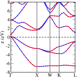
Despite the statements contained within Eqs.(13) and (14) being obviously true, the inversion of the target densities from LDA and GGAs remains nonetheless insightful as a benchmark to quantify the numerical error from the minimisation algorithm outlined in section IV, since the LXC potential from the DFA (or DFA-LXC potential for short), is known a priori to the inversion. We first performed a self-consistent calculation of the target density and KS potential (see Eq. (4)) by self-consistently solving the KS equations for the LDA and PBE functionals and obtained the band structure for these functionals (using ). The LDA and PBE band gaps are given in Table 1. We found that the LXC-LDA111 For LDA target densities, the LXC potential was initialised to the PBE potential calculated from the target density. If the LXC potential was instead initialised to the LDA potential calculated from the target density like elsewhere in this work, the inversion is already converged without any further iteration, and more importantly remains converged. and LXC-PBE band structures were indistinguishable from the LDA and PBE band structures for all systems considered, with the mean absolute deviation (MAD) between the LXC-DFA and DFA band gap being around 3 meV for both LDA and PBE. An example of this is shown in Fig. 3 for GaAs using the PBE target density where the LXC-PBE band structure is indistinguishable from the PBE band structure. An example of the inversion of the LDA density in diamond is given in the supplemental material[88].
| LDA | PBE | rSCAN | B3LYP | PBE0 | HSE06 | HF | expt. | ||||||
| BAs222Experimental band gap from Ref.[89] | |||||||||||||
| BP | |||||||||||||
| C(diamond) | |||||||||||||
| CaO | |||||||||||||
| CdS(wurtzite) | |||||||||||||
| CdS(zincblende) | |||||||||||||
| CdSe | |||||||||||||
| GaAs | |||||||||||||
| GaP | |||||||||||||
| Ge | |||||||||||||
| InP | |||||||||||||
| LiF | |||||||||||||
| MgO | |||||||||||||
| NaCl | |||||||||||||
| Si | |||||||||||||
| SiC | |||||||||||||
| ZnS | |||||||||||||
| 333Lattice parameters from Ref.[90], expt. band gap from Ref.[91] | |||||||||||||
| 444Lattice parameters from Refs.[92, 93], expt. band gap from Ref.[94] | |||||||||||||
| 555Lattice parameters from Refs.[95, 96], expt. band gap from Ref.[97] | |||||||||||||
| 666Lattice parameters from Refs.[98, 99], expt. band gap from Ref.[100] | |||||||||||||
| 777Lattice parameters from Refs.[101], expt. band gap from Ref.[102] | |||||||||||||
| MAE | |||||||||||||
| MARE | |||||||||||||
| MAD | 0.20 | 1.12 | 1.42 | 0.83 | 6.90 | ||||||||
| MARD | 14.6% | 36.9% | 40.7% | 28.9% | 68.6% | ||||||||
IV.2 LXC-Hartree-Fock(HF) or Local Fock Exchange(LFX)
In contrast to the KS orbitals which are density optimal[66], the HF orbitals are energy optimal in the sense they optimise the Slater determinant that minimises the HF energy functional. The (unconstrained) minimisation of the HF functional yields single-particle equations which contain a non-local potential in the form of the Fock exchange operator
| (15) |
In a wider sense HF together with hybrid DFAs can be considered within a GKS scheme wherein the GKS equations are single-particle equations with a non-local exchange potential as part of the full XC potential . Alternatively, these DFAs can be considered within a KS scheme with a local XC potential but due to the orbital dependence, one cannot evaluate Eq. (1) directly and instead the OEP method must be used.
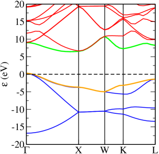
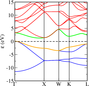
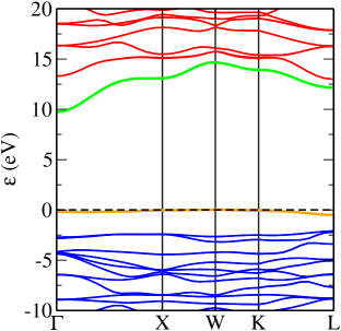
Table 1 gives the HF and LFX band gaps for various systems. As expected, the HF band gap is typically a massive overestimate of the experimental band gaps. In the literature, this effect is often attributed to the lack of correlation [103], but see the discussion in Ref. [104]. The LXC potential obtained by the inversion of the HF density is the local Fock exchange[64] (LFX) potential . As a result of the strongly non-local nature of the HF exchange potential , the band structures obtained from will naturally be quite different from the original HF band structure obtained via , unlike the LXC-LDA and LXC-PBE band structures where the potentials obtained by inversion, and . In contrast to HF, the LFX band gaps are generally a systematic improvement over the unphysically large HF band gaps, when compared to experiment. As discussed in Refs.[64, 68], the LFX potential is expected to be similar to the xOEP potential in weakly interacting systems whose exchange energy is much larger than the correlation energy. Therefore, the LFX band structures and band gaps obtained here and in Refs.[64, 68] will be similar to those calculated using xOEP[69, 70, 71, 43, 72].
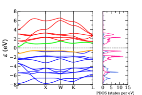
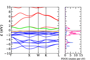
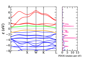
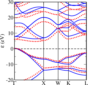
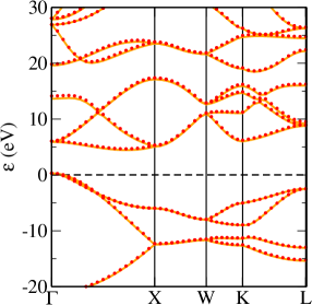
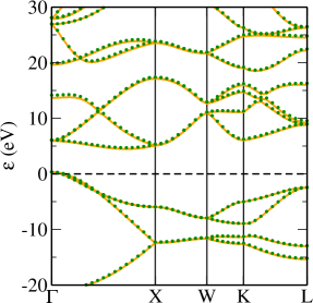
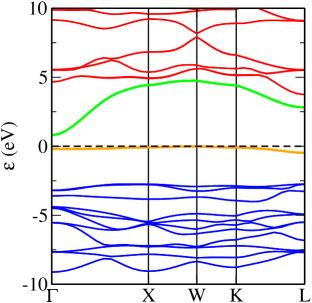
In particular for Si, shown in Fig. 4 the LFX band gap happens to be equal to the experimental band gap of while the HF band gap is . In the case of Ge, local and semi-local DFAs[105, 106] like LDA and PBE incorrectly predict it to be metallic rather than insulating. On the other hand, the LFX potential correctly describes Ge qualitatively, with a gap , suggesting that the failure of the LDA and PBE potentials is probably due to an inaccurate description of exchange. Alternatively, these results can be improved by resorting to many-body perturbation theory techniques such as the method[107, 108, 109]. We note that large relative errors were obtained for LFX in GaAs (39%) and ZnS (42%).
In the case of the cubic perovskites , and , we found that the computed LFX band gap was an overestimate in contrast to the other semiconductors and insulators in Table 1, although the same qualitative improvement over HF was observed. Comparable overestimates in these cubic perovskites were obtained in the xOEP calculations by Betzinger et al.[110] and Trushin et al.[73]. As discussed in the latter, the error is not necessarily due to an inherent shortcoming of the xOEP/LFX potentials but rather to additional physical effects not considered here such as zero-point motion of the lattice that leads to band gap renormalisation. In transition metal perovskites such as , this can be as large as as calculated in Ref. [111], although the effect is largely insignificant in other semiconductors and insulators (see Ref. [112]).
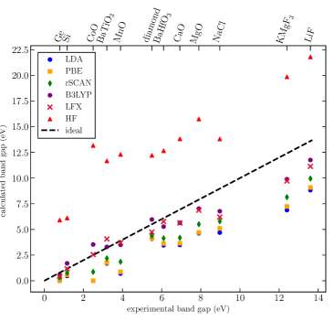
Finally, as shown in Fig. 5, the degree to which the LFX band gap underestimates the fundamental band gap increases in systems with large fundamental gaps. In particular, LiF, NaCl and had absolute errors of , and respectively which were larger than LFX’s mean absolute error (MAE) of for the materials in Table 1. However, the absolute relative errors of 19.7% and 21.6% for LiF and respectively, remain comparable to mean absolute relative error (MARE) of LFX while NaCl has an absolute relative error of 30.8%.
IV.3 Reducing non-locality: Hybrid Functionals
We have seen in section IV.1 that the LXC potential obtained from the inversion of LDA and PBE densities is identical to the original potential LDA and PBE KS potentials, and . At the other end of the non-locality spectrum, in the previous section, we have shown that a target density generated by the non-local HF (exchange-only) potential results in an LXC potential with improved band structures and particularly band gaps compared to the HF results. The natural question is what happens when the two are combined.
In hybrid functionals, the exchange energy is a mixture of non-local Fock exchange and local/semi-local DFA exchange energy. Considered in a GKS scheme, this gives rise to a non-local exchange potential that is not as strongly non-local as the full HF exchange potential due to a smaller weighting on the Fock exchange energy in the total energy functional. We considered target densities from three hybrid functionals: B3LYP[78, 79, 80], PBE0[81] and HSE[83] (we specifically used the HSE06[82] parametrization).
In all hybrid functionals considered, the LXC band gap obtained by the inversion of the respective hybrid target densities was lower than the calculated GKS band gap. This behaviour of the LXC potential is analogous to the behaviour of the LFX potential , although the effect is reduced due to the smaller weighting of HF exchange in the full exchange energy .
The B3LYP functional mixes several exchange and correlation functionals with HF exchange ,
| (16) |
is the Becke-88[113] (B88) gradient-correction (to the LSDA) and is the correlation functional of Lee, Yang and Parr[114] (LYP) with[78] and . The only term in Eq. (16) that gives rise to a non-local potential in a GKS scheme is the HF exchange energy while all other terms are all explicitly local/semi-local density functionals which yield a local, multiplicative potential. The LXC-B3LYP band gaps differ from the GKS-B3LYP band gaps with a mean absolute relative deviation (MARD) of 34% and a mean absolute deviation (MAD) of whereas the MARD and MAD for HF and LFX were 68.6% and respectively, thereby highlighting the weaker non-locality in B3LYP. We also note that the LXC-B3LYP band gaps were still typically larger than the LDA and PBE band gaps. The reason for this is two-fold; the first is the aforementioned analogous behaviour of to . The second is the semi-local B88 functional constructed as a correction to the L(S)DA which, as noted by Becke[113], obtains a greater portion of the full exchange energy due to the recovering the correct asymptotic behaviour of the exchange energy density.
We stress that the non-linearity of the inversion process means that the LXC potential does not simply subtract off the non-local HF potential and replace it with the LFX potential. Notably, in the case of Ge, the LXC-B3LYP potential gives a metallic band structure whereas the GKS-B3LYP band gap is 0.54 eV; the latter is closer to the experimental value of 0.785 eV than the LFX band gap of 0.46 eV. We also found that the LXC-B3LYP band gaps were similar to the GKS-rSCAN band gaps where the MAD between the two was 0.13 eV and the MARD was 7.18%. We will explore this in detail in section IV.5.
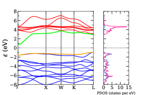
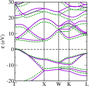
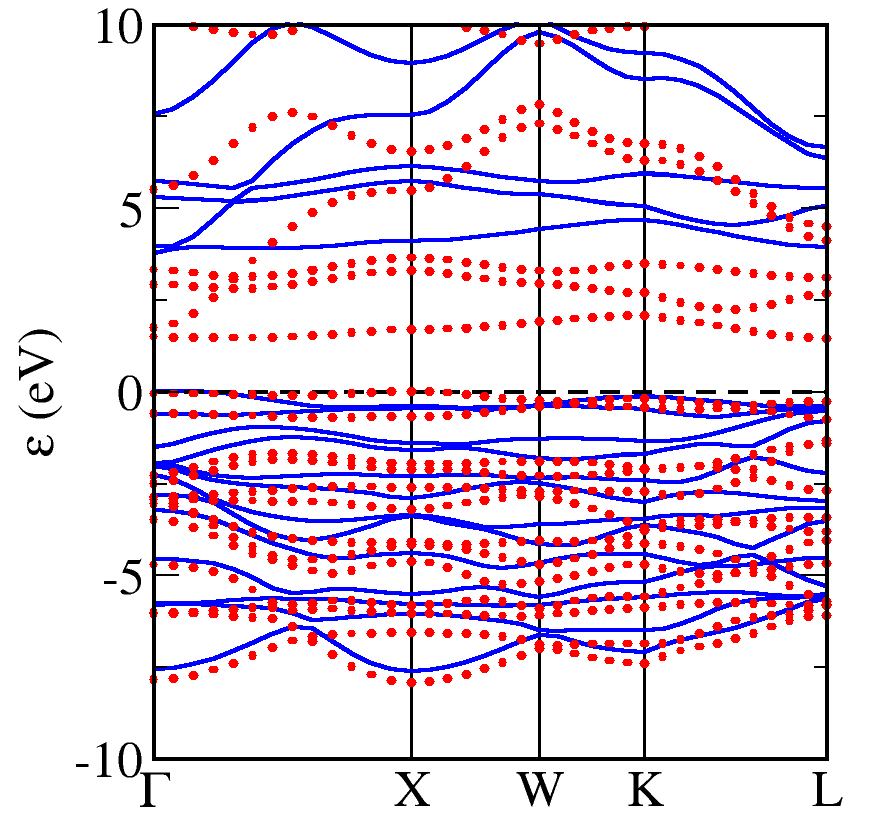
In the case of PBE0, which contains non-local HF exchange with the remainder of the XC energy coming from semi-local PBE, one might expect the LXC band gap to be similar to the PBE band gap with the LXC potential similar to the PBE potential. Indeed, this is the case as shown in Fig. 6b for diamond where the LXC band structure obtained by inversion of the PBE0 target density is virtually identical to the PBE band structure. Likewise, the remainder of Table 1 shows that the LXC-PBE0 band gap is close (but not necessarily identical) to the PBE gap, with the MAD and MARD between the two being 0.36 eV and 19.8% respectively. Some notable deviations between LXC-PBE0 and PBE include Ge, in which LXC-PBE0 gave a small (but non-zero nonetheless) band gap of 0.20 eV in contrast to PBE as well as LXC-B3LYP, which predicted it to be metallic. Larger-than-average absolute deviations between LXC-PBE0 and PBE of 0.51 eV, 0.67 eV and 0.68 eV were also observed in CaO, MgO and LiF respectively, as well as in cubic perovskites with an absolute deviation of 0.55 eV for being the smallest and the largest of 0.60 eV for .
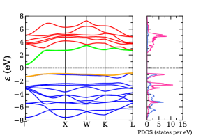
Turning our attention to a range-separated hybrid such as HSE06, the short-range exchange (a mixture of HF non-local exchange and PBE semi-local exchange) is screened by PBE exchange at long-range. Since we have a different DFA from PBE0, it is not clear in advance how the densities and thus the LXC potentials from HSE06 and PBE0 will differ, in particular the degree to which screening in the former will affect the density and potential. Indeed, there is a MAD of 0.60 eV and MARD of 18.32% between HSE06 and PBE0 GKS gaps for the semiconductors and insulators in Table 1, which is unsurprising due to the screened Fock operator in the former which can lead to potentially large differences in the GKS eigenvalues.
However, it turns out that for the systems we considered, there was only a small difference in the LXC-PBE0 and LXC-HSE06 band gaps with a MAD of (and a MARD 1.2%) between the two. The similarity of the two LXC potentials from PBE0 and HSE06, and , to each other suggests that both DFAs yield similar densities. Given the similarity of LXC-PBE0 to PBE, by extension, both these DFAs have similar densities to PBE and their respective LXC potentials are similar to the PBE potential . In particular, it appears that the screening within the HSE06 DFA has a minimal effect on the density compared to unscreened PBE0. Together with the fact that both HSE06 and PBE0 have the same weighting of Fock exchange (25%), it is not too surprising that the inversion of an HSE06 target density, , yields a similar band structure to the inversion of the corresponding PBE0 target density for these systems. This is shown in Figs. 6c and 6d for diamond. The similarity of the LXC band structures thus suggests that the and are similar. The difference in band gaps obtained when these two DFAs are considered in a GKS scheme is thus due to the screening of HF exchange in HSE06 that is absent in PBE0. Therefore, despite having similar densities, the two DFAs yield different GKS band gaps, notably in where GKS-PBE0 gives and GKS-HSE06 gives , while the LXC band gaps obtained for the respective target densities remain similar at around .
IV.3.1 Total Energy Differences and Band Gaps
The inversion of a DFA’s density finds the local Kohn-Sham potential that reproduces that DFA’s density.
As discussed in section II.1, the orbitals obtained by solving the Kohn-Sham equations with
do not fully minimise the total energy for a non-local DFA due to the additional constraint that the potential obtained from the inversion must be local.
Therefore, the total energy difference between and can thus be used as a metric to gauge the degree of non-locality in a particular GKS scheme.
| HF(LFX) | B3LYP | |
|---|---|---|
| BAs | 0.390 | 0.016 |
| BP | 0.179 | 0.005 |
| C-diamond | 0.152 | 0.006 |
| CaO | 0.255 | 0.014 |
| CdS (zincblende) | 0.347 | 0.016 |
| CdSe | 0.644 | 0.023 |
| GaAs | 0.536 | 0.023 |
| GaP | 0.348 | 0.011 |
| Ge | 0.519 | 0.020 |
| InP | 0.449 | 0.012 |
| LiF | 0.093 | 0.005 |
| MgO | 0.112 | 0.005 |
| NaCl | 0.109 | 0.007 |
| Si | 0.228 | 0.009 |
| SiC | 0.140 | 0.005 |
| ZnS | 0.371 | 0.013 |
| 0.664 | 0.023 | |
| 0.840 | 0.044 | |
| 0.664 | 0.038 | |
| 0.290 | 0.016 | |
| 0.777 | 0.044 |
Table 2 gives total energy differences for HF and B3LYP when evaluated using the GKS orbitals and LXC orbitals obtained via the KS equations with XC potential set to the LXC potential as defined in Eq. (11). As one might expect, the total energy difference between LFX (LXC-HF) and HF is the largest since HF contains a strongly non-local exchange-only potential. Moreover, these energy differences are similar but not identical to those between xOEP and HF[64]. We note that the xOEP potential satisfies the virial relation for exchange[115] while LFX satisfies the virial relation only approximately to second order[64]. Turning now to B3LYP which contains only 20% HF exchange, the constraint of a local potential is less “severe” and thus the orbitals generated by are closer to the energy optimal GKS orbitals generated by the non-local GKS potential . This can also be inferred from the smaller changes in the band structure between LXC-B3LYP and GKS-B3LYP compared to LFX and HF.
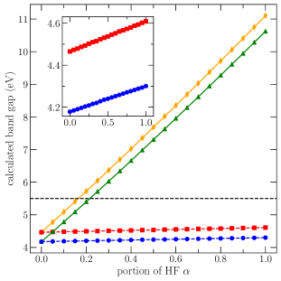
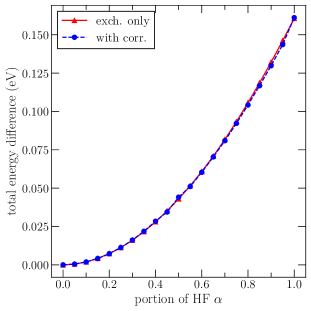
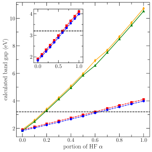
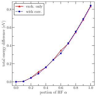
To better investigate the effects of non-locality on both the band structure and total energy difference, we considered a PBE0-like hybrid functional with parameter
| (17) |
where gives the standard PBE0 functional. For various values of , the DFA defined by Eq. (17) was treated in a GKS scheme from which the GKS band gap and target density were obtained before inversion to obtain the LXC potential and band gap.
The results are shown in Figs. 7 and 8 for diamond and respectively with and without the inclusion of semi-local PBE correlation .
At low , the total energy difference is small (zero at ) but increases rapidly in a non-linear fashion as , i.e. full HF exchange. The GKS band gap increases faster than the LXC band gap with , where at in the absence of correlation, one obtains the LFX gap. We note that the inclusion of semi-local PBE correlation does not significantly change the difference in total energies although it does result in a reduction of both the GKS and LXC band gaps.
The difference in exchange-only band gaps and those with semi-local PBE correlation exhibits a weak dependence on with the difference between the two for a given remaining nearly constant; in diamond the difference in LXC band gaps between exchange-only results varied between 0.29–0.31 eV and 0.08–0.12 eV in . The connection between band gap and total energy is not fully clear; in particular, a larger difference in the total energies does not necessarily directly translate to a larger difference between GKS and LXC band gaps. For , see Fig. 8 and Tables 1 and 2, the HF gap is 11.67 eV and the LFX gap is with a difference of 7.6 eV between the two while the total energy difference of the HF functional when evaluated using the LFX and HF orbitals is 0.840 eV. By contrast, for diamond, see Fig. 7, the HF gap is 12.21 eV and the LFX gap is 4.75 eV with the two differing by yet the total energy difference is only , more than a factor of 5 smaller than the energy difference for despite both systems having similar band gap differences between HF and LFX.
At high , one might expect that the inclusion of correlation would give a calculated LXC band gap closer to the experimental value. However, we note that while LFX (and xOEP) treat exchange exactly, DFAs can still remain accurate in spite of the inexact treatment of exchange due to a cancellation of errors when the corresponding exchange and correlation DFAs are used in tandem, in this case, PBE exchange with PBE correlation. We note the KS gap does not equal the fundamental gap, with the two differing by the exchange-correlation derivative discontinuity discussed in greater detail in section V.
IV.3.2 Transition Metal Monoxides (TMOs)
| LDA | PBE | rSCAN | B3LYP | PBE0 | HSE06 | HF | expt. | ||||||
| CoO | 111Value from Ref. [117] | ||||||||||||
| FeO | – | – | – | 222Value from Refs. [118, 119] | |||||||||
| MnO | 333Value from Ref. [120] | ||||||||||||
| NiO | 444Value from Ref. [121] | ||||||||||||
| MAE | |||||||||||||
| MARE | |||||||||||||
| MAD | - | - | 0.10 | 1.88 | 2.39 | 1.82 | 9.01 | ||||||
| MARD | - | - | 6.2% | 49.6% | 53.7% | 46.8% | 77.4 | ||||||
The transition metal monoxides (TMOs) (Co,Fe,Mn,Ni)O, which adopt an AFM-II ([111]) insulating ground state present challenges for simple local and semi-local density functionals due to strong inter-electron interactions, particularly for -electrons. These interactions lead to strong localisation that is often underestimated by these functionals as a result of their tendency to overly delocalise electrons due to the presence of self-interaction error (SIE)[10, 11, 12, 122, 13] leading to the prediction of both quantitatively as well as qualitatively incorrect material properties. HF on the other hand does not have SIE and by extension, hybrid functionals which include a portion of HF exchange are able to partly correct the SIE[119, 123]. These errors can also be corrected through DFT+ (discussed in the next section), xOEP[124, 43] as well as many-body perturbation theory methods such as the approximation[125] and dynamical mean field theory[126, 127, 128, 129] (DMFT).
The band gaps for various DFAs and the corresponding LXC gaps are given in Table 3 for these TMOs in the rocksalt structure. For MnO and NiO, the LSDA underestimate the band gap when compared to experiment with LSDA giving 0.81 eV compared to the experimental value of 3.9 eV for MnO[120] and 0.66 eV compared to the experimental value[121] of 4.0 eV for NiO. A small improvement is given using a GGA such as PBE with for MnO and 1.23 eV for NiO. However, in the case of CoO and FeO, the inaccuracy of the LSDA and PBE is more severe with both systems predicted to be falsely metallic rather than insulating. In the case of a meta-generalised gradient approximation (meta-GGA) such as the regularised variant of the strongly constrained and appropriately normed functional[130] (rSCAN), all four TMOs were correctly predicted to be insulating which is unsurprising given the SCAN functional is expected to have a smaller SIE than GGAs[131, 132, 133].
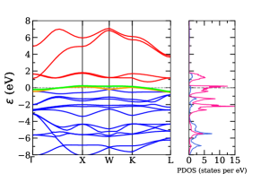
The LFX potential, by virtue of being obtained by inversion of the HF density, does not contain a SIE. It is thus unsurprising perhaps that the computed KS band gap using LFX had the lowest MAE of and MARE of 17.6% compared to experiment, with accuracy comparable to hybrid functionals treated in a GKS scheme, in particular B3LYP and HSE06. On the other hand, a larger deviation between LFX and the experimental band gap was found in FeO, shown in Fig. 9, where LFX gave a gap of 0.81 eV while the experimental gap is 2.4 eV. We believe this is due to strong Mott physics, which we will address in section V. We point out that the qualitative picture is correct and in particular, we are not aware of another local XC potential (besides LFX/xOEP) which predicts a finite band gap for FeO. In the other TMOs studied, the similarity of the LFX band gaps and experimental band gaps suggests weaker Mott physics and that the failure of local and semi-local DFAs is at least partially due to an inaccurate or incomplete description of exchange.
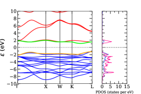
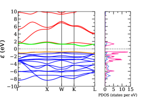
The inversion of PBE0 and HSE06 target densities in these TMOs, however, yields an LXC potential that is quite different from the PBE potential. Notably, in the case of CoO, both the LXC-PBE0 and LXC-HSE06 band structures (shown in Fig. 10) are insulating with a band gap of 1.45 eV and 1.44 eV respectively while PBE predicts it to be metallic. Likewise, the LXC-B3LYP potential gives a band gap of 1.30 eV which is perhaps not surprising since the weighting for HF exchange in the B3LYP, PBE0 and HSE06 functionals is similar with 20% in B3LYP and 25% in PBE0 and HSE06 (the non-locality is weaker in HSE06 since the HF exchange is screened by PBE exchange at long range). Similar albeit less drastic differences were observed for MnO and NiO; in these systems, PBE gives the right qualitative behaviour but underestimates the band gaps giving 0.96 eV and 1.23 eV respectively. However, LXC-PBE0 and LXC-HSE06 give band gaps of 2.02 eV and 2.01 eV in MnO and 2.72 eV and 2.71 eV in NiO. The behaviour of the LXC potential for PBE0 and HSE06 densities for (Co,Ni,Mn)O is thus consistent with the behaviour in the previously discussed systems in Table 1 insofar that PBE0 and HSE06 appear to give similar densities and therefore similar LXC potentials. However, the large difference between these LXC potentials and the PBE potential suggests that the PBE0 and HSE06 densities differ greatly from the PBE density, especially in CoO where the SIE is large.
| Structure | HF(LFX) | B3LYP |
|---|---|---|
| CoO | 1.522 | 0.126 |
| FeO | 0.496 | – |
| MnO | 0.740 | 0.047 |
| NiO | 1.516 | 0.104 |
Table 4 gives the differences in total energies for HF and B3LYP when the respective total energy functional is evaluated using the LFX/LXC orbitals and HF/GKS orbitals as defined in Eq. (11). In the TMOs studied in this work, we found that the total energies differences were typically larger than the other systems studied for both B3LYP and HF, cf. Table 2. CoO had the largest difference for both HF and B3LYP of 1.522 eV and 0.126 eV respectively; MnO had the smallest difference for B3LYP of 0.104 eV while FeO had the smallest energy difference out of all TMOs for HF of 0.496 eV. For comparison, the largest total energy difference for the other systems in Table 2 was with energy differences of 0.777 eV and 0.044 eV for LFX and B3LYP respectively. The larger-than-average values obtained for TMOs suggest that the degree of non-locality for HF and B3LYP when treated in a GKS scheme in these systems is stronger compared to the previous systems studied.
IV.4 Reduced Non-Locality: LDA+
The Hubbard model[134, 135, 136] is the simplest model Hamiltonian that is capable of capturing a Mott transition. In the so-called DFT+ method, the ‘Hubbard-’ term from the Hubbard model gives an energy contribution to a subset of orbitals that penalises the double occupancy resulting in greater localisation of the electrons occupying these orbitals. This partially corrects the delocalisation error and SIE exhibited particularly in local and semi-local DFAs, with the role of the Hubbard- term in the total energy expression analogous to that of HF in hybrid functionals. More recently, Koopmans-compliant[137, 138, 139, 140] functionals have been developed to tackle the issue of SIE within standard DFAs through a restoration of the piecewise-linearity condition known from exact DFT as obtained by Perdew, Parr, Levy and Balduz[141]. Since the Hubbard- correction in DFT+ is applied to a subset of all orbitals (typically strongly-correlated and electrons in most calculations), it is by definition a non-local potential and thus the LXC potential derived from a DFT+ target density will naturally differ from the original, self-consistent non-local potential for DFT+ or GKS potential .
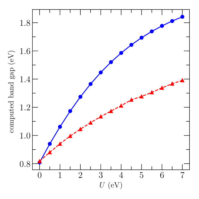
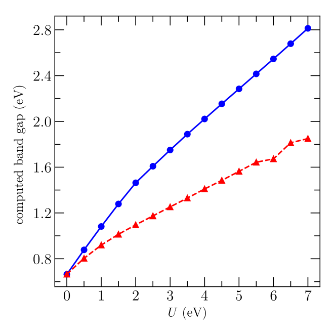
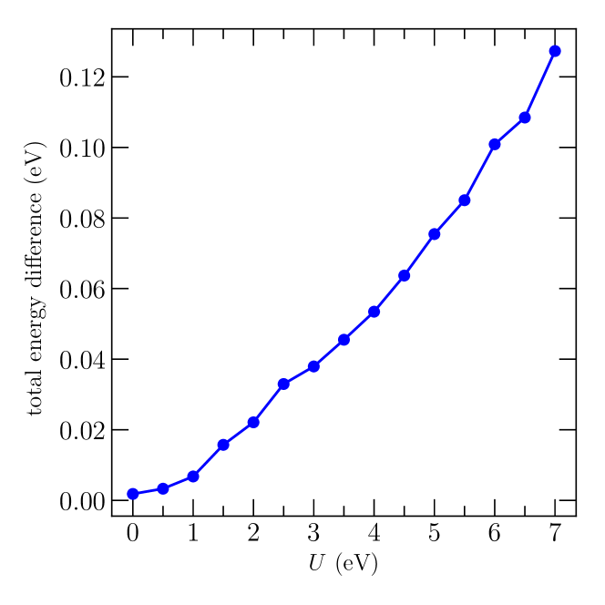
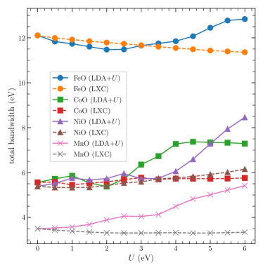
We performed LDA+ band structure calculations for (Co,Mn,Ni,Fe)O in the rocksalt structure (with the same lattice parameters as the previous calculations) with a Hubbard- applied to the -orbitals of the respective metal cation across a range of from 0–7 eV. We then inverted the obtained LDA+ densities to find the LXC-LDA+ potential . Figs. 11a and 11b gives the calculated LDA+ and LXC-LDA+ band gap as a function of the Hubbard- parameter for MnO and NiO respectively. In both systems, one is unable to obtain the experimental band gap with LDA+ with a giving for MnO compared to the experimental gap of 3.9 eV and 2.81 eV for NiO compared to the experimental gap of . As a recurring theme throughout this work, the LXC band gap is always lower than the LDA+ band gap with the LXC-LDA+ gap for being about 75%–80% of the LDA+ gap for MnO while it was 65%–73% of the LDA+ gap in NiO. We note that for MnO, the rate of change in the band gap as a function of starts to decrease at high as there is a limit to the localisation that can be achieved in the -electrons. We would expect similar behaviour at even higher in NiO as well. For completeness, we point out that there is an ‘optimal’ or appropriate value for Hubbard- for each TMO although the determination of this value lies beyond the scope of this work and we instead draw attention to methods developed for this purpose elsewhere based on linear response(see Refs. [142, 143]). More recently, these methods have been reformulated using the machinery of density functional perturbation theory (DFPT)[144, 145].
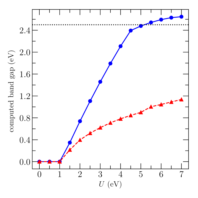
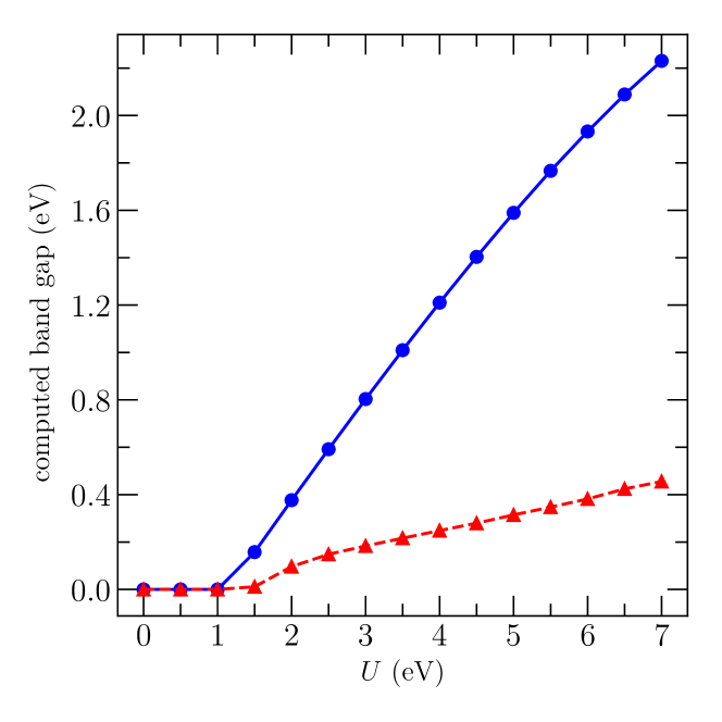
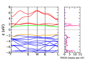
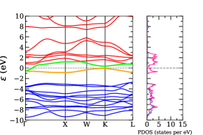
Both FeO and CoO are falsely predicted to be metallic by the LDA. When LDA+ is used, there exists a “critical” value of , denoted , at which both systems exhibit a metal-insulator transition. The variation of the band gap as a function of Hubbard- is shown in Figs. 12a and 12b for CoO and FeO respectively. The value of resulting in a non-zero gap is the same for both the LXC-LDA+ and LDA+ calculations in CoO. However, in FeO, the value of for LXC-LDA+ lagged behind the LDA+ value with and for LDA+ and LXC-LDA+ respectively. This behaviour, particularly in CoO, shows that causes a change in the density from the usual LDA density. Consequently, the LXC potential obtained by the inversion of the LDA+ target density necessarily differs from the non-local self-consistent LDA+ potential. We also note that while the gap opens up in the standard LDA+ calculation at the same , i.e. , for both FeO and CoO, the rate at which the gap increases is faster in CoO than FeO. Moreover, it is possible to obtain the experimental band gap of 2.5 eV of CoO by using eV with LDA+ but this is not possible with LXC-LDA+; as a whole, we found that for eV that the LXC-LDA+ band was around 40% to 50% of the LDA+ band gap in CoO. In contrast to the other TMOs, the LXC-LDA+ band gap for FeO does not change significantly across the range of between and considered in this work, changing only by in FeO compared to 0.92 eV in CoO. In particular, we found that the LXC band gap for FeO was less than 25% of the LDA+ band gap.
In a similar fashion to the HF and B3LYP functionals, total energy differences can be used to quantify the degree of non-locality of the LDA+ potential.
We calculate the total energy difference when the LDA+ functional
is evaluated using the self-consistent orbitals and the orbitals that are eigenstates of the single-particle KS Hamiltonian with the LXC potential. In both instances, the same value of Hubbard- is utilised when evaluating the total energy functional.
Fig. 13 shows the results of this procedure for FeO where we note the difference is 0.0455 eV at eV and 0.127 eV at eV.
For comparison, the energy difference between LFX and HF for FeO was 0.496 eV.
The fact that the difference between LFX and HF is larger than the difference between LXC-LDA+ and LDA+ suggests LDA+ has weaker non-locality.
This is not surprising as the non-local HF exchange operator acts on all occupied orbitals that comprise the HF determinant while the Hubbard- is only applied to a subset of the orbitals, namely those with -character, that comprise the KS determinant .
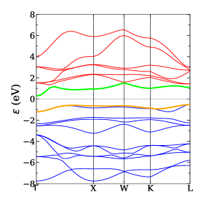
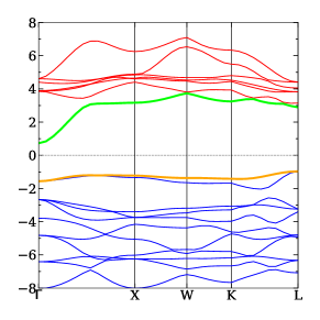
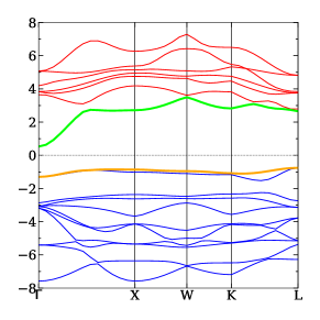
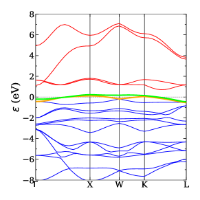
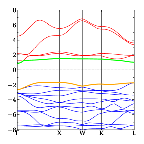
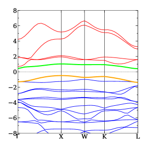
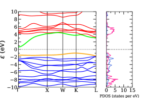
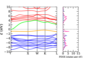
Moreover, we now draw attention to the more noteworthy differences in the dispersion of the energy bands between LXC-LDA+ and LDA+ band structures. In LDA+, a sufficiently large leads to the unphysical flattening of bands due to over localisation of electrons to which the is applied (in this case the electrons). This is shown in Fig. 14 for MnO where the LDA, LDA+ and LXC-LDA+ band structures are plotted at . Intriguingly, the inversion restores some of the original energy dispersion of the LDA band structure for the occupied states although the LXC-LDA+ gap is higher than the original LDA gap. However, for unoccupied states, both the LXC and LDA+ band structures have a similar conduction band width of while the LDA band structure has a conduction band width of in addition to all three having different band gaps as previously stated. Examining the LDA+ band structure of CoO shown in Fig. 14 for eV, one can similarly find flat bands due to over-localisation. However, the inversion does not nearly restore the energy dispersion of the occupied states in CoO compared to MnO. In yet another contrast to MnO, the conduction band width of CoO was found to be similar across all three methods where the LDA band width was 0.68 eV, LDA+ 0.66 eV, and LXC-LDA+ 0.62 eV for eV. On the other hand, the valence band width between the LXC-LDA+ and LDA+ band structures were similar, and respectively, but LDA had a valence band width of 0.65 eV.
Investigating how the total occupied band width varies across these methods is non-trivial due to the difference in how the potentials act on the orbital. As previously stated, the LXC potential acts on all orbitals in an identical manner but the LDA+ potential in general does not. We calculated the projected density of states (PDOS) using OptaDOS[146, 147] using the population analysis methodology of Segall et al.[148] for both the LDA+ and LXC-LDA+ (PDOS calculations presented in supplemental material[88]) and found that the LXC potential largely preserves the character of each band, while LDA+ does not, particularly where the valence band starts to acquire oxygen character in addition to that of the transition metal cation character due to hybridisation. The number of bands that contribute to the total -character is thus in general not the same between the LDA+ and LXC-LDA+ results. For these reasons, in Fig. 15, we plot the total band width of bands below and including the valence band with (predominantly) character at the LDA level of theory, denoted ,
| (18) |
In both the LDA and LXC-LDA+ cases, corresponds to the number of electrons in the respective transition metal cation (although a notable exception is in FeO[88]). We emphasise that unlike LDA+, the total band width of the same set of bands is insensitive to the value of Hubbard- which can be attributed to the local nature of the LXC potential which acts on all orbitals in the same way. Moreover, we also point out that the does not significantly change from the LDA, i.e. value with changing in contrast to LDA+, reflecting our previous observations for the band structures of CoO and MnO, cf. Fig. 14.
IV.5 Weak Non-Locality: Meta-GGA densities
The final class of densities we consider in this work are those generated via GKS calculations with meta-generalised gradient approximations (meta-GGAs), particularly using the rSCAN functional. Like other orbital functionals which are implicit functionals of the density, meta-GGAs can also be treated via the OEP method similar to xOEP in which case the resulting KS potential is local . We consider a GKS scheme in this work since the resulting potential obtained is non-local and we wish to investigate the degree of non-locality in the GKS potential .
In general, we found that LXC-rSCAN band structures were similar to the GKS-rSCAN band structures (cf. Tables 1 and 3) where we found that the MAD between the GKS-rSCAN and LXC-rSCAN band gaps was about 0.17 eV. The largest difference in band gap between the two potentials was obtained for GaAs where the GKS-rSCAN band gap was 0.89 eV and 0.43 eV in LXC-rSCAN. Similar differences were obtained for InP with GKS-rSCAN giving 1.01 eV and LXC-rSCAN giving 0.58 eV while for NaCl where the GKS-rSCAN band gap was 5.79 eV compared to the LXC-rSCAN band gap of 5.34 eV. This suggests that the non-locality of the GKS rSCAN potential is weak.
This is exemplified in the results for Ge where LXC-rSCAN gave a metallic band structure while GKS-rSCAN gave a band gap of 0.31 eV. Recall however for Ge that if the target density is obtained via a GKS scheme featuring a more strongly non-local potential such as HF or even PBE0 and HSE06, the LXC potential obtained from inversion of this density gave a finite band gap, with LXC-PBE0 and LXC-HSE06 giving 0.20 eV and 0.18 eV respectively. On the other hand, LXC-B3LYP for Ge gives a metallic band structure.
Interestingly, we also find that the LXC-rSCAN band gaps and band structures are similar to the LXC results for hybrid functionals for weakly correlated systems cf. Table 1. We found that the MAD between the LXC-rSCAN and LXC-B3LYP was around 0.13 eV while the MARD between them was 7.18%. A similar result was found between LXC-PBE0 and LXC-HSE06, and LXC-rSCAN. For comparison, the MAD between B3LYP and LXC-B3LYP was 1.15 eV with the MARD being 33.7% while the MAD between LXC-PBE0 and LXC-HSE06 with PBE was around 0.36 eV with a MARD of around 20%. This suggests that the densities of hybrid functionals are similar given that they yield similar LXC potentials and band structures. The differences thus obtained in a GKS scheme are due to exchange, more precisely the degree of non-locality in the exchange potential . In strongly correlated systems such as the TMOs, the differences are larger and in these instances, the LXC band gap for a hybrid functional is not close to the LXC-rSCAN band gap with the former typically being higher. NiO is an exception where LXC-B3LYP gave a band gap of 2.52 eV while LXC-rSCAN gave a band gap of 2.61 eV. Moreover, we find a larger difference in the band gap and band structure between GKS-rSCAN and LXC-rSCAN in these instances.
V Exchange-Correlation Derivative Discontinuity
As shown by Perdew and others[141, 149, 2, 3], it is known that the KS gap between the valence band maximum (VBM) and conduction band minimum (CBM) of the exact KS system is not equal to the fundamental gap of the actual solid due to the so-called exchange-correlation derivative discontinuity
| (19) |
In this work, we have calculated various KS potentials, which we dubbed LXC potentials, via inversion of their target densities; the question we address is what is the value of for the various LXC potentials obtained. Although an ab initio calculation of is beyond the scope of this study (via the total energy of the electron and electron systems), it is still possible to make some comments or estimate the size of for various potentials. It has been shown[150] that local and semi-local DFAs with local multiplicative XC potentials have zero/vanishing . However, we note that it is possible to get a non-zero via an ensemble generalisation of such DFAs, for instance as done by Kraisler and Kronik[151, 152] although this correction vanishes in the thermodynamic limit.
The LFX potential obtained from the inversion of the HF density is expected to be similar to the xOEP potential, especially in weakly correlated systems (stronger deviations between LFX and xOEP were found by Hollins et al[43, 64] in the TMOs). Both the LFX and xOEP potentials are exchange-only potentials; as such, when the total energy for LFX/xOEP is obtained at the HF level, i.e. omitting any correlation which may be added as a post-SCF step, then the only contribution to is from the exchange discontinuity . Ab initio calculations for in xOEP in the literature[69, 71, 72] show that the magnitude of restores the HF band gap. The magnitude of for the LFX potential is similar. We note that a correlation discontinuity, , can be calculated using a post-HF method, whose magnitude, at least in second-order Møller–Plesset (MP2) is comparable or can even exceed (see Refs. [153, 154, 155]).
For GKS schemes, it has been proposed that the GKS band gap is equal to, or more precisely, can be interpreted as the fundamental gap[14]. With hybrid functionals, one can consider to be the difference between the GKS and the LXC band gap. This likewise includes LDA+ and meta-GGAs[67] although as the result of the weaker non-locality in GKS, the difference between LXC and GKS band gaps is smaller, and thus the resulting magnitude of is smaller than in hybrid functionals.
With regard to strongly correlated systems, namely Mott insulators, the hallmark of a Mott insulator is a large correction relative to the KS band gap, or equivalently that the majority of the contribution to the fundamental gap is from . In FeO we found that the LFX band gap had a larger-than-average absolute relative error to the experimental gap. We believe that the fact the LFX gap greatly underestimates the experimental fundamental gap confirms the strong Mott physics at play in FeO and that the correlation energy not taken into account by both HF and LFX is significant. Conversely, in the other TMOs, the similarity of the LFX band gap to the size of the experimental gap suggests that the failure of local and semi-local DFAs is due to the inaccurate, or rather incomplete description of exchange.
VI Conclusions
We have presented a thorough study across a range of solids of the KS potential with a local exchange-correlation (LXC) potential term obtained via the inversion of target densities from various DFAs employing a non-local potential in a GKS scheme. Our calculations provide a means of quantifying the strength of the non-locality in various GKS schemes, which we achieved by comparing the computed KS band structures with GKS band structures using HF, hybrid functionals, LDA+ functionals and meta-GGAs.
In general, we found that the exchange-only local Fock exchange (LFX) potential, obtained from the inversion of the HF density gives KS band gaps that have the best agreement with experimental fundamental gaps out of any LXC potential (omitting any exchange and correlation derivative discontinuity correction). We also point out that the LFX potential is almost indistinguishable to the exchange-only OEP (xOEP) calculations[64, 43, 69, 70, 71, 124, 72, 73], particularly in weakly correlated systems, although we expect stronger deviations in strongly correlated systems, for instance in the TMOs studied in this work. These LFX (KS) band gaps are also comparable in accuracy to those of hybrid DFAs when treated in GKS, with slightly reduced computational cost for the LFX band structure and associated spectroscopic calculations due to the use of a local potential. We also note that to the best of our knowledge, the LFX potential as well as the xOEP are, to our knowledge, the only local potentials which qualitatively predict FeO to be insulating rather than metallic, highlighting that the failure of potentials from local and semi-local DFAs in strongly correlated systems is at least partial failing to correct for SIE.
In hybrid schemes, the reduced contribution from the Fock exchange term results in GKS potential with a weaker non-locality. Consequently, although the LXC band gap is still lower than the corresponding GKS band gap for a given DFA (analogous to the behaviour between HF and LFX), we find that the difference between the two is smaller. In meta-GGAs, there is an even smaller difference between the LXC and GKS results highlighting that the non-locality for meta-GGAs due to the kinetic energy density is even weaker.
We also presented an alternative means of quantifying this non-locality by evaluating the total energy functional for a given DFA using the GKS and LXC orbitals and obtaining the energy difference between the two. We found that the energy differences were typically an order of magnitude smaller for the B3LYP functional compared to the HF functional; naturally the GKS orbitals yield a lower total energy minimum given that the minimisation is carried out without the constraint of a local potential.
Moreover, our results highlight that it is possible for different DFAs to give similar densities and thus similar LXC/KS potentials although they give different GKS potentials. For instance, in weakly correlated systems, we found that the LXC results for PBE0 and HSE06 were similar to PBE suggesting that the improved band gap prediction of these hybrid DFAs is due to the the non-locality in the GKS potential contributed by the non-local Fock exchange term. We observed similar behaviour between LXC-rSCAN and the LXC results for hybrid DFAs, notably LXC-B3LYP, suggesting that the improvement in the gap within GKS is a result of the stronger non-locality in B3LYP compared to rSCAN.
On the other hand, in strongly correlated systems, such as the anti ferromagnetic TMOs considered in this work, LXC-PBE0 and LXC-HSE06 have a greater discrepancy with PBE, leading to an improved density in the former as a result of correcting SIE through an accurate treatment of exchange. This is reflected in the larger total energy differences when the HF and B3LYP energy functionals are evaluated using GKS and LXC orbitals. Taken as a whole, these results imply that GKS and KS will yield similar densities where exchange effects dominate over correlation.
The LXC-LDA+ results for CoO and FeO in particular highlight the importance of correcting for self-interaction. At sufficiently large Hubbard-, the LXC potential obtained from the inversion of the LDA+ density does not qualitatively predict these systems to be falsely metallic, reflecting the role of the Hubbard- as a correction for self-interaction error[142, 143]. The weaker non-locality from the Hubbard- can be seen with the smaller total energy difference in FeO for LDA+ compared to HF across the range of we considered when evaluated using GKS and LXC orbitals.
Finally, it is well-known that the exact KS band gap is not equal to the fundamental gap of a solid. The difference between the two is the exchange-correlation derivative discontinuity[141, 149] . As discussed in Ref.[14], the difference between a KS treatment, in this case, the LXC result, and GKS treatment gives an estimate of , although we find that the size of obtained in this manner is small, particularly in rSCAN as a result of the weaker non-locality.
Although we have specifically studied the KS potentials from various DFAs in this work, our algorithm is general and robust and can be readily applied to densities from other electronic structure methods, for example, quantum Monte Carlo (QMC), such that the local potential obtained via inversion of an accurate density can give insight into features of the exact KS potential[9]. Comparing the results of the inversion of QMC densities with the existing LXC results will enable the benchmarking of DFAs with regards to the densities they yield and by extension, their LXC potentials in keeping with the original spirit of KS-DFT, namely to provide an accurate density through a mean-field local effective potential.
The data that supports the findings of this article will be made available through Durham collections[156].
Acknowledgements.
V Ravindran acknowledges the Durham Doctoral Scholarship programme for financial support. We acknowledge the use of the Durham Hamilton HPC service (Hamilton) and the UK national supercomputing facility (ARCHER2) funded by EPSRC grant EP/X035891/1.References
- Kohn and Sham [1965] W. Kohn and L. J. Sham, “Self-Consistent Equations Including Exchange and Correlation Effects,” Phys. Rev. 140, A1133–A1138 (1965).
- Sham and Schlüter [1983] L. J. Sham and M. Schlüter, “Density-Functional Theory of the Energy Gap,” Phys. Rev. Lett. 51, 1888–1891 (1983).
- Godby, Schlüter, and Sham [1986] R. W. Godby, M. Schlüter, and L. J. Sham, “Accurate Exchange-Correlation Potential for Silicon and Its Discontinuity on Addition of an Electron,” Phys. Rev. Lett. 56, 2415–2418 (1986).
- Godby, Schlüter, and Sham [1987a] R. W. Godby, M. Schlüter, and L. J. Sham, “Quasiparticle energies in GaAs and AlAs,” Phys. Rev. B 35, 4170–4171 (1987a).
- Godby, Schlüter, and Sham [1987b] R. W. Godby, M. Schlüter, and L. J. Sham, “Trends in self-energy operators and their corresponding exchange-correlation potentials,” Phys. Rev. B 36, 6497–6500 (1987b).
- Godby, M., and Sham [1988] R. W. Godby, S. M., and L. J. Sham, “Self-energy operators and exchange-correlation potentials in semiconductors,” Phys. Rev. B 37, 10159–10175 (1988).
- Hohenberg and Kohn [1964] P. Hohenberg and W. Kohn, “Inhomogeneous Electron Gas,” Phys. Rev. 136, B864–B871 (1964).
- Gidopoulos [2011] N. I. Gidopoulos, “Progress at the interface of wave-function and density-functional theories,” Phys. Rev. A 83, 040502 (2011).
- Aouina et al. [2023] A. Aouina, M. Gatti, S. Chen, S. Zhang, and L. Reining, “Accurate Kohn-Sham auxiliary system from the ground-state density of solids,” Phys. Rev. B 107, 195123 (2023).
- Perdew and Zunger [1981] J. P. Perdew and A. Zunger, “Self-interaction correction to density-functional approximations for many-electron systems,” Phys. Rev. B 23, 5048–5079 (1981).
- Svane and Gunnarsson [1990] A. Svane and O. Gunnarsson, “Transition-metal oxides in the self-interaction–corrected density-functional formalism,” Phys. Rev. Lett. 65, 1148–1151 (1990).
- Mori-Sánchez, Cohen, and Yang [2008] P. Mori-Sánchez, A. J. Cohen, and W. Yang, “Localization and delocalization errors in density functional theory and implications for band-gap prediction,” Phys. Rev. Lett. 100, 146401 (2008).
- Bryenton et al. [2023] K. R. Bryenton, A. A. Adeleke, S. G. Dale, and E. R. Johnson, “Delocalization error: The greatest outstanding challenge in density-functional theory,” WIREs Computational Molecular Science 13, e1631 (2023).
- Perdew et al. [2017] J. P. Perdew, W. Yang, K. Burke, Z. Yang, E. K. U. Gross, M. Scheffler, G. E. Scuseria, T. M. Henderson, I. Y. Zhang, A. Ruzsinszky, H. Peng, J. Sun, E. Trushin, and A. Görling, “Understanding band gaps of solids in generalized Kohn–Sham theory,” Proc. Natl. Acad. Sci. USA 114, 2801–2806 (2017).
- Wang et al. [2021] A. Wang et al., “A framework for quantifying uncertainty in DFT energy corrections,” Sci. Rep. 11, 15496 (2021).
- Cohen, Mori-Sánchez, and Yang [2012] A. J. Cohen, P. Mori-Sánchez, and W. Yang, “Challenges for Density Functional Theory,” Chem. Rev. 112, 289–320 (2012).
- Burke [2012] K. Burke, “Perspective on density functional theory,” The Journal of Chemical Physics 136, 150901 (2012).
- Vuckovic and Burke [2020] S. Vuckovic and K. Burke, “Quantifying and Understanding Errors in Molecular Geometries,” J. Chem. Phys. Lett. 11, 9957–9964 (2020).
- Vuckovic [2022] S. Vuckovic, “Quantification of Geometric Errors Made Simple: Application to Main-Group Molecular Structures,” J. Phys. Chem. A 126, 1300–1311 (2022).
- De Waele et al. [2016] S. De Waele, K. Lejaeghere, M. Sluydts, and S. Cottenier, “Error estimates for density-functional theory predictions of surface energy and work function,” Phys. Rev. B 94, 235418 (2016).
- Brittain et al. [2009] D. R. B. Brittain, C. Y. Lin, A. T. B. Gilbert, E. I. Izgorodina, P. M. W. Gill, and M. L. Coote, “The role of exchange in systematic DFT errors for some organic reactions,” Phys. Chem. Chem. Phys. 11, 1138–1142 (2009).
- Kim, Sim, and Burke [2013] M.-C. Kim, E. Sim, and K. Burke, “Understanding and Reducing Errors in Density Functional Calculations,” Phys. Rev. Lett. 111, 073003 (2013).
- Kim, Sim, and Burke [2014] M.-C. Kim, E. Sim, and K. Burke, “Ions in solution: Density corrected density functional theory (DC-DFT),” J. Chem. Phys 140, 18A528 (2014).
- Vuckovic et al. [2019] S. Vuckovic, S. Song, J. Kozlowski, E. Sim, and K. Burke, “Density Functional Analysis: The Theory of Density-Corrected DFT,” J. Chem. Theory Comput 15, 6636–6646 (2019).
- Sim et al. [2022] E. Sim, S. Song, S. Vuckovic, and K. Burke, “Improving Results by Improving Densities: Density-Corrected Density Functional Theory,” J. Am. Chem. Soc 144, 6625–6639 (2022).
- Song et al. [2022] S. Song, S. Vuckovic, E. Sim, and K. Burke, “Density-Corrected DFT Explained: Questions and Answers,” J. Chem. Theory Comput 18, 817–827 (2022).
- Nam et al. [2020] S. Nam, S. Song, E. Sim, and K. Burke, “Measuring Density-Driven Errors Using Kohn–Sham Inversion,” J. Chem. Theory Comput 16, 5014–5023 (2020).
- Dasgupta et al. [2021] S. Dasgupta, E. Lambros, J. P. Perdew, and F. Paesani, “Elevating density functional theory to chemical accuracy for water simulations through a density-corrected many-body formalism,” Nat Commun 12, 6359 (2021).
- Dasgupta et al. [2022] S. Dasgupta, C. Shahi, P. Bhetwal, J. P. Perdew, and F. Paesani, “How Good Is the Density-Corrected SCAN Functional for Neutral and Ionic Aqueous Systems, and What Is So Right about the Hartree–Fock Density?” J. Chem. Theory Comput 18, 4745–4761 (2022).
- Kaplan et al. [2023] A. D. Kaplan, C. Shahi, P. Bhetwal, R. K. Sah, and J. P. Perdew, “Understanding Density-Driven Errors for Reaction Barrier Heights,” J. Chem. Theory Comput 19, 532–543 (2023).
- Song et al. [2023] S. Song, S. Vuckovic, Y. Kim, H. Yu, E. Sim, and K. Burke, “Extending density functional theory with near chemical accuracy beyond pure water,” Nat. Commun 14, 799 (2023).
- Yu et al. [2023] H. Yu, S. Song, S. Nam, K. Burke, and E. Sim, “Density-Corrected Density Functional Theory for Open Shells: How to Deal with Spin Contamination,” J. Phys. Chem. Lett. 14, 9230–9237 (2023).
- Talman and Shadwick [1976] J. D. Talman and W. F. Shadwick, “Optimized effective atomic central potential,” Phys. Rev. A 14, 36–40 (1976).
- Sharp and Horton [1953] R. T. Sharp and G. K. Horton, “A Variational Approach to the Unipotential Many-Electron Problem,” Phys. Rev. 90, 317–317 (1953).
- Yang and Wu [2002] W. Yang and Q. Wu, “Direct Method for Optimized Effective Potentials in Density-Functional Theory,” Phys. Rev. Lett. 89, 143002 (2002).
- Wu and Yang [2003] Q. Wu and W. Yang, “A direct optimization method for calculating density functionals and exchange–correlation potentials from electron densities,” J. Chem. Phys 118, 2498–2509 (2003).
- Görling [1992] A. Görling, “Kohn-Sham potentials and wave functions from electron densities,” Phys. Rev. A 46, 3753–3757 (1992).
- Erhard, Trushin, and Görling [2022] J. Erhard, E. Trushin, and A. Görling, “Numerically stable inversion approach to construct Kohn–Sham potentials for given electron densities within a Gaussian basis set framework,” J. Chem. Phys. 156, 204124 (2022).
- Perdew et al. [2005] J. P. Perdew, A. Ruzsinszky, J. Tao, V. N. Staroverov, G. E. Scuseria, and G. I. Csonka, “Prescription for the design and selection of density functional approximations: More constraint satisfaction with fewer fits,” J. Chem. Phys 123, 062201 (2005).
- Kümmel and Kronik [2008] S. Kümmel and L. Kronik, “Orbital-dependent density functionals: Theory and applications,” Rev. Mod. Phys. 80, 3–60 (2008).
- Gidopoulos and Lathiotakis [2012] N. I. Gidopoulos and N. N. Lathiotakis, “Nonanalyticity of the optimized effective potential with finite basis sets,” Phys. Rev. A 85, 052508 (2012).
- Heaton-Burgess, Bulat, and Yang [2007] T. Heaton-Burgess, F. A. Bulat, and W. Yang, “Optimized Effective Potentials in Finite Basis Sets,” Phys. Rev. Lett. 98, 256401 (2007).
- Hollins et al. [2012] T. W. Hollins, S. J. Clark, K. Refson, and N. I. Gidopoulos, “Optimized effective potential using the Hylleraas variational method,” Phys. Rev. B 85, 235126 (2012).
- Kümmel and Perdew [2003] S. Kümmel and J. P. Perdew, “Optimized effective potential made simple: Orbital functionals, orbital shifts, and the exact Kohn-Sham exchange potential,” Phys. Rev. B 68, 035103 (2003).
- Jensen and Wasserman [2018] D. S. Jensen and A. Wasserman, “Numerical methods for the inverse problem of density functional theory,” Int. J. Quantum Chem 118, e25425 (2018).
- Shi and Wasserman [2021] Y. Shi and A. Wasserman, “Inverse Kohn–Sham Density Functional Theory: Progress and Challenges,” J. Phys. Chem. Lett 12, 5308–5318 (2021).
- Werden and Davidson [1984] S. H. Werden and E. R. Davidson, “On the Calculation of Potentials from Densities,” in Local Density Approximations in Quantum Chemistry and Solid State Physics, edited by J. P. Dahl and J. Avery (Springer US, Boston, MA, 1984) pp. 33–42.
- Chan, Tozer, and Handy [1997] G. K.-L. Chan, D. J. Tozer, and N. C. Handy, “Correlation potentials and functionals in Hartree-Fock-Kohn-Sham theory,” J. Chem. Phys. 107, 1536–1543 (1997).
- van Leeuwen and Baerends [1994] R. van Leeuwen and E. J. Baerends, “Exchange-correlation potential with correct asymptotic behavior,” Phys. Rev. A 49, 2421–2431 (1994).
- Zhao, Morrison, and Parr [1994] Q. Zhao, R. C. Morrison, and R. G. Parr, “From electron densities to Kohn-Sham kinetic energies, orbital energies, exchange-correlation potentials, and exchange-correlation energies,” Phys. Rev. A 50, 2138–2142 (1994).
- Savin, Umrigar, and Gonze [1998] A. Savin, C. Umrigar, and X. Gonze, “Relationship of Kohn–Sham eigenvalues to excitation energies,” Chemical Physics Letters 288, 391–395 (1998).
- Peirs, Van Neck, and Waroquier [2003] K. Peirs, D. Van Neck, and M. Waroquier, “Algorithm to derive exact exchange-correlation potentials from correlated densities in atoms,” Phys. Rev. A 67, 012505 (2003).
- Kadantsev and Stott [2004] E. S. Kadantsev and M. J. Stott, “Variational method for inverting the Kohn-Sham procedure,” Phys. Rev. A 69, 012502 (2004).
- Ryabinkin and Staroverov [2012] I. G. Ryabinkin and V. N. Staroverov, “Determination of Kohn–Sham effective potentials from electron densities using the differential virial theorem,” J. Chem. Phys 137, 164113 (2012).
- Kumar, Singh, and Harbola [2019] A. Kumar, R. Singh, and M. K. Harbola, “Universal nature of different methods of obtaining the exact Kohn–Sham exchange-correlation potential for a given density,” J. Phys. B: At. Mol. Opt. Phys. 52, 075007 (2019).
- Callow, Lathiotakis, and Gidopoulos [2020] T. J. Callow, N. N. Lathiotakis, and N. I. Gidopoulos, “Density-inversion method for the Kohn–Sham potential: Role of the screening density,” J. Chem. Phys 152, 164114 (2020).
- Bousiadi, Gidopoulos, and Lathiotakis [2022] S. Bousiadi, N. I. Gidopoulos, and N. N. Lathiotakis, “Density inversion method for local basis sets without potential auxiliary functions: inverting densities from RDMFT,” Phys. Chem. Chem. Phys. 24, 19279–19286 (2022).
- Görling and Ernzerhof [1995] A. Görling and M. Ernzerhof, “Energy differences between Kohn-Sham and Hartree-Fock wave functions yielding the same electron density,” Phys. Rev. A 51, 4501–4513 (1995).
- Ryabinkin, Kananenka, and Staroverov [2013] I. G. Ryabinkin, A. A. Kananenka, and V. N. Staroverov, “Accurate and Efficient Approximation to the Optimized Effective Potential for Exchange,” J. Chem. Phys. 111, 013001 (2013).
- Kohut, Ryabinkin, and Staroverov [2014] S. V. Kohut, I. G. Ryabinkin, and V. N. Staroverov, “Hierarchy of model Kohn–Sham potentials for orbital-dependent functionals: A practical alternative to the optimized effective potential method,” J. Chem. Phys. 140, 18A535 (2014).
- Holas et al. [1993] A. Holas, N. H. March, Y. Takahashi, and C. Zhang, “Hartree-Fock method posed as a density-functional theory: Application to the Be atom,” Phys. Rev. A 48, 2708–2715 (1993).
- Nagy [1997] A. Nagy, “Alternative derivation of the Krieger-Li-Iafrate approximation to the optimized-effective-potential method,” Phys. Rev. A 55, 3465–3468 (1997).
- Jiqiang Chen and Stott [1994] R. O. E. Jiqiang Chen and M. J. Stott, “Exchange-correlation potential for small atoms,” Philos. mag., B 69, 1001–1009 (1994).
- Hollins et al. [2017] T. W. Hollins, S. J. Clark, K. Refson, and N. I. Gidopoulos, “A local Fock-exchange potential in Kohn–Sham equations,” J. Phys.: Condens. Matter 29, 04LT01 (2017).
- Fletcher and Reeves [1964] R. Fletcher and C. M. Reeves, “Function minimization by conjugate gradients,” Comput. J 7, 149–154 (1964).
- Kohn [1999] W. Kohn, “Nobel lecture: Electronic structure of matter—wave functions and density functionals,” Rev. Mod. Phys. 71, 1253–1266 (1999).
- Yang et al. [2016] Z.-H. Yang, H. Peng, J. Sun, and J. P. Perdew, “More realistic band gaps from meta-generalized gradient approximations: Only in a generalized Kohn-Sham scheme,” Phys. Rev. B 93, 205205 (2016).
- Clark et al. [2017] S. J. Clark, T. W. Hollins, K. Refson, and N. I. Gidopoulos, “Self-interaction free local exchange potentials applied to metallic systems,” J. Phys.: Condens. Matter 29, 374002 (2017).
- Städele et al. [1997] M. Städele, J. A. Majewski, P. Vogl, and A. Görling, “Exact Kohn-Sham Exchange Potential in Semiconductors,” Phys. Rev. Lett. 79, 2089–2092 (1997).
- Städele et al. [1999] M. Städele, M. Moukara, J. A. Majewski, P. Vogl, and A. Görling, “Exact exchange Kohn-Sham formalism applied to semiconductors,” Phys. Rev. B 59, 10031–10043 (1999).
- Grüning, Marini, and Rubio [2006] M. Grüning, A. Marini, and A. Rubio, “Density functionals from many-body perturbation theory: The band gap for semiconductors and insulators,” J. Chem. Phys, 124, 154108 (2006).
- Klimeš and Kresse [2014] J. Klimeš and G. Kresse, “Kohn-Sham band gaps and potentials of solids from the optimised effective potential method within the random phase approximation,” J. Chem. Phys. 140, 054516 (2014).
- Trushin, Fromm, and Görling [2019] E. Trushin, L. Fromm, and A. Görling, “Assessment of the exact-exchange-only Kohn-Sham method for the calculation of band structures for transition metal oxide and metal halide perovskites,” Phys. Rev. B 100, 075205 (2019).
- Clark et al. [2005] S. J. Clark, M. D. Segall, C. J. Pickard, P. J. Hasnip, M. I. J. Probert, K. Refson, and M. C. Payne, “First principles methods using CASTEP,” Z. Kristall. 220, 567–570 (2005).
- Car and Parrinello [1985] R. Car and M. Parrinello, “Unified Approach for Molecular Dynamics and Density-Functional Theory,” Phys. Rev. Lett. 55, 2471–2474 (1985).
- Monkhorst and Pack [1976] H. J. Monkhorst and J. D. Pack, “Special points for Brillouin-zone integrations,” Phys. Rev. B 13, 5188–5192 (1976).
- Lejaeghere et al. [2016] K. Lejaeghere et al., “Reproducibility in density functional theory calculations of solids,” Science 351, aad3000 (2016).
- Becke [1993] A. D. Becke, “Density-functional thermochemistry. III. The role of exact exchange,” J. Chem. Phys. 98, 5648–5652 (1993).
- Lee, Yang, and Parr [1988a] C. Lee, W. Yang, and R. G. Parr, “Development of the Colle-Salvetti correlation-energy formula into a functional of the electron density,” Phys. Rev. B 37, 785–789 (1988a).
- Stephens et al. [1994] P. J. Stephens, F. J. Devlin, C. F. Chabalowski, and M. J. Frisch, “Ab initio calculation of vibrational absorption and circular dichroism spectra using density functional force fields,” J. Phys. Chem. 98, 11623–11627 (1994).
- Perdew, Ernzerhof, and Burke [1996] J. P. Perdew, M. Ernzerhof, and K. Burke, “Rationale for mixing exact exchange with density functional approximations,” J. Chem. Phys. 105, 9982–9985 (1996).
- Heyd, Scuseria, and Ernzerhof [2006] J. Heyd, G. E. Scuseria, and M. Ernzerhof, “Erratum: ‘Hybrid functionals based on a screened Coulomb potential’ [J. Chem. Phys. 118, 8207 (2003)],” J. Chem. Phys. 124 (2006).
- Heyd, Scuseria, and Ernzerhof [2003] J. Heyd, G. E. Scuseria, and M. Ernzerhof, “Hybrid functionals based on a screened Coulomb potential,” J. Chem. Phys 118, 8207–8215 (2003).
- Perdew, Burke, and Ernzerhof [1996] J. P. Perdew, K. Burke, and M. Ernzerhof, “Generalized Gradient Approximation Made Simple,” Phys. Rev. Lett. 77, 3865–3868 (1996).
- Madelung [1996] O. Madelung, Semiconductors – Basic Data, 2nd ed. (Springer Berlin / Heidelberg, Berlin, Heidelberg, 1996).
- Perdew and Schmidt [2001] J. P. Perdew and K. Schmidt, “Jacob’s ladder of density functional approximations for the exchange-correlation energy,” AIP Conf Proc 577, 1–20 (2001).
- Note [1] For LDA target densities, the LXC potential was initialised to the PBE potential calculated from the target density. If the LXC potential was instead initialised to the LDA potential calculated from the target density like elsewhere in this work, the inversion is already converged without any further iteration, and more importantly remains converged.
- [88] See supplemental material at DOI:XXXXXXX for the inversion of the LDA density and projected density of states that show how we selected bands with predominantly -character in calculations for transition metal oxides.
- Kang et al. [2019] J. S. Kang, M. Li, H. Wu, H. Nguyen, and Y. Hu, “Basic physical properties of cubic boron arsenide,” Appl. Phys. Lett. 115 (2019).
- Li et al. [2004] L. Li, B. J. Kennedy, Y. Kubota, K. Kato, and R. F. Garrett, “Structures and phase transitions in perovskites,” J. Mater. Chem. 14, 263–273 (2004).
- Kim et al. [2017] Y. M. Kim, C. Park, T. Ha, U. Kim, N. Kim, J. Shin, Y. Kim, J. Yu, J. H. Kim, and K. Char, “High-k perovskite gate oxide BaHfO3,” APL Mater 5 (2017), 016104.
- Hellwege and Hellwege [1969] K. H. Hellwege and A. M. Hellwege, “Ferroelectrics and related substances,” in Landolt-Börnstein, Vol. 3 (Springer-Verlag, 1969).
- Wang et al. [2010] J. J. Wang, F. Y. Meng, X. Q. Ma, M. X. Xu, and L. Q. Chen, “Lattice, elastic, polarization, and electrostrictive properties of BaTiO3 from first-principles,” J. Appl. Phys 108 (2010), 034107.
- Wemple [1970] S. H. Wemple, “Polarization Fluctuations and the Optical-Absorption Edge in BaTi,” Phys. Rev. B 2, 2679–2689 (1970).
- Levin et al. [2003] I. Levin, T. G. Amos, S. M. Bell, L. Farber, T. A. Vanderah, R. S. Roth, and B. H. Toby, “Phase equilibria, crystal structures, and dielectric anomaly in the BaZrO3–CaZrO3 system,” J. Chem. Phys. 175, 170–181 (2003).
- Evarestov [2011] R. A. Evarestov, “Hybrid density functional theory LCAO calculations on phonons in Ba(Ti,Zr,Hf)3,” Phys. Rev. B 83, 014105 (2011).
- Robertson [2000] J. Robertson, “Band offsets of wide-band-gap oxides and implications for future electronic devices,” J. Vac. Sci. Technol. B 18, 1785–1791 (2000).
- Heaton and Lin [1982a] R. A. Heaton and C. C. Lin, “Electronic energy-band structure of the KMg crystal,” Phys. Rev. B 25, 3538–3549 (1982a).
- Luaña, Costales, and Martín Pendás [1997] V. Luaña, A. Costales, and A. Martín Pendás, “Ions in crystals: The topology of the electron density in ionic materials.ii. the cubic alkali halide perovskites,” Phys. Rev. B 55, 4285–4297 (1997).
- Heaton and Lin [1982b] R. A. Heaton and C. C. Lin, “Electronic energy-band structure of the KMg crystal,” Phys. Rev. B 25, 3538–3549 (1982b).
- Abramov et al. [1995] Y. A. Abramov, V. G. Tsirelson, V. E. Zavodnik, S. A. Ivanov, and B. I. D., “The chemical bond and atomic displacements in SrTiO3 from X-ray diffraction analysis,” Acta Crystallographica Section B 51, 942–951 (1995).
- van Benthem, Elsässer, and French [2001] K. van Benthem, C. Elsässer, and R. H. French, “Bulk electronic structure of SrTiO3: Experiment and theory,” J. Appl. Phys 90, 6156–6164 (2001).
- Ashcroft and Mermin [1976] N. W. Ashcroft and N. D. Mermin, Solid State Physics (Saunders College Publishing, 1976).
- Blair, Kroukis, and Gidopoulos [2015] A. I. Blair, A. Kroukis, and N. I. Gidopoulos, “A correction for the Hartree-Fock density of states for jellium without screening,” J. Chem. Phys 142 (2015), 10.1063/1.4909519.
- Bachelet and Christensen [1985] G. B. Bachelet and N. E. Christensen, “Relativistic and core-relaxation effects on the energy bands of gallium arsenide and germanium,” Phys. Rev. B 31, 879–887 (1985).
- Ekuma et al. [2013] C. Ekuma, M. Jarrell, J. Moreno, and D. Bagayoko, “Re-examining the electronic structure of germanium: A first-principle study,” Physics Letters A 377, 2172–2176 (2013).
- Hedin [1965] L. Hedin, “New Method for Calculating the One-Particle Green’s Function with Application to the Electron-Gas Problem,” Phys. Rev. 139, A796–A823 (1965).
- Rohlfing, Krüger, and Pollmann [1993] M. Rohlfing, P. Krüger, and J. Pollmann, “Quasiparticle band-structure calculations for C, Si, Ge, GaAs, and SiC using Gaussian-orbital basis sets,” Phys. Rev. B 48, 17791–17805 (1993).
- Fleszar [2001] A. Fleszar, “LDA, GW, and exact-exchange Kohn-Sham scheme calculations of the electronic structure of semiconductors,” Phys. Rev. B 64, 245204 (2001).
- Betzinger et al. [2012] M. Betzinger, C. Friedrich, A. Görling, and S. Blügel, “Precise response functions in all-electron methods: Application to the optimized-effective-potential approach,” Phys. Rev. B 85, 245124 (2012).
- Bhandari et al. [2018] C. Bhandari, M. van Schilfgaarde, T. Kotani, and W. R. L. Lambrecht, “All-electron quasiparticle self-consistent band structures for including lattice polarization corrections in different phases,” Phys. Rev. Mater. 2, 013807 (2018).
- Karsai et al. [2018] F. Karsai, M. Engel, E. Flage-Larsen, and G. Kresse, “Electron–phonon coupling in semiconductors within the GW approximation,” New J. Phys. 20, 123008 (2018).
- Becke [1988] A. D. Becke, “Density-functional exchange-energy approximation with correct asymptotic behavior,” Phys. Rev. A 38, 3098–3100 (1988).
- Lee, Yang, and Parr [1988b] C. Lee, W. Yang, and R. G. Parr, “Development of the Colle-Salvetti correlation-energy formula into a functional of the electron density,” Phys. Rev. B 37, 785–789 (1988b).
- Levy and Perdew [1985] M. Levy and J. P. Perdew, “Hellmann-feynman, virial, and scaling requisites for the exact universal density functionals. shape of the correlation potential and diamagnetic susceptibility for atoms,” Phys. Rev. A 32, 2010–2021 (1985).
- Sasaki, Fujino, and Tákeuchi [1979] S. Sasaki, K. Fujino, and Y. Tákeuchi, “X-Ray Determination of Electron-Density Distributions in Oxides, MgO, MnO, CoO, and NiO, and Atomic Scattering Factors of their Constituent Atoms,” Proc. Jpn. Acad., Ser. B 55, 43–48 (1979).
- van Elp et al. [1991] J. van Elp et al., “Electronic structure of CoO, Li-doped CoO, and ,” Phys. Rev. B 44, 6090–6103 (1991).
- Parmigiani and Sangaletti [1999] F. Parmigiani and L. Sangaletti, “Fine structures in the X-ray photoemission spectra of MnO, FeO, CoO, and NiO single crystals,” J Electron Spectros Relat Phenomena. 98-99, 287–302 (1999).
- Tran et al. [2006] F. Tran, P. Blaha, K. Schwarz, and P. Novák, “Hybrid exchange-correlation energy functionals for strongly correlated electrons: Applications to transition-metal monoxides,” Phys. Rev. B 74, 155108 (2006).
- Zimmermann et al. [1999] R. Zimmermann et al., “Electronic structure of 3d-transition-metal oxides: on-site Coulomb repulsion versus covalency,” J. Phys. Condens. Matter 11, 1657 (1999).
- Sawatzky and Allen [1984] G. A. Sawatzky and J. W. Allen, “Magnitude and Origin of the Band Gap in NiO,” Phys. Rev. Lett. 53, 2339–2342 (1984).
- Himmetoglu et al. [2014] B. Himmetoglu, A. Floris, S. de Gironcoli, and M. Cococcioni, “Hubbard-corrected DFT energy functionals: The LDA+U description of correlated systems,” Int. J. Quantum Chem. 114, 14–49 (2014).
- Gillen and Robertson [2013] R. Gillen and J. Robertson, “Accurate screened exchange band structures for the transition metal monoxides MnO, FeO, CoO and NiO,” J. Phys.: Condens. Matter 25, 165502 (2013).
- Engel and Schmid [2009] E. Engel and R. N. Schmid, “Insulating ground states of transition-metal monoxides from exact exchange,” Phys. Rev. Lett. 103, 036404 (2009).
- Sakuma and Aryasetiawan [2013] R. Sakuma and F. Aryasetiawan, “First-principles calculations of dynamical screened interactions for the transition metal oxides O (=Mn, Fe, Co, Ni),” Phys. Rev. B 87, 165118 (2013).
- Kotliar et al. [2006] G. Kotliar, S. Y. Savrasov, K. Haule, V. S. Oudovenko, O. Parcollet, and C. A. Marianetti, “Electronic structure calculations with dynamical mean-field theory,” Rev. Mod. Phys. 78, 865–951 (2006).
- Kuneš et al. [2008] J. Kuneš, A. V. Lukoyanov, V. I. Anisimov, R. T. Scalettar, and W. E. Pickett, “Collapse of magnetic moment drives the Mott transition in MnO,” Nature Materials 7, 198–202 (2008).
- Mandal et al. [2019a] S. Mandal, K. Haule, K. M. Rabe, and D. Vanderbilt, “Systematic beyond-DFT study of binary transition metal oxides,” Npj Comput. Mater. 5, 115 (2019a).
- Mandal et al. [2019b] S. Mandal, K. Haule, K. M. Rabe, and D. Vanderbilt, “Influence of magnetic ordering on the spectral properties of binary transition metal oxides,” Phys. Rev. B 100, 245109 (2019b).
- Bartók and Yates [2019] A. P. Bartók and J. R. Yates, “Regularized SCAN functional,” J. Chem. Phys 150 (2019), 10.1063/1.5094646, 161101.
- Sai Gautam and Carter [2018] G. Sai Gautam and E. A. Carter, “Evaluating transition metal oxides within DFT-SCAN and frameworks for solar thermochemical applications,” Phys. Rev. Mater. 2, 095401 (2018).
- Long, Sai Gautam, and Carter [2020] O. Y. Long, G. Sai Gautam, and E. A. Carter, “Evaluating optimal for transition-metal oxides within the SCAN+ framework,” Phys. Rev. Mater. 4, 045401 (2020).
- Sun, Ruzsinszky, and Perdew [2015] J. Sun, A. Ruzsinszky, and J. P. Perdew, “Strongly Constrained and Appropriately Normed Semilocal Density Functional,” Phys. Rev. Lett. 115, 036402 (2015).
- Hubbard and Flowers [1963] J. Hubbard and B. H. Flowers, “Electron correlations in narrow energy bands,” Proc. R. Soc. Lond. A 276, 238–257 (1963).
- Tasaki [1998a] H. Tasaki, “From Nagaoka’s Ferromagnetism to Flat-Band Ferromagnetism and Beyond: An Introduction to Ferromagnetism in the Hubbard Model,” Prog. Theor. Phys. 99, 489–548 (1998a).
- Tasaki [1998b] H. Tasaki, “The Hubbard model - an introduction and selected rigorous results,” J. Phys. Condens. Matter 10, 4353 (1998b).
- Dabo et al. [2010] I. Dabo, A. Ferretti, N. Poilvert, Y. Li, N. Marzari, and M. Cococcioni, “Koopmans’ condition for density-functional theory,” Phys. Rev. B 82, 115121 (2010).
- Nguyen et al. [2018] N. L. Nguyen, N. Colonna, A. Ferretti, and N. Marzari, “Koopmans-compliant spectral functionals for extended systems,” Phys. Rev. X 8, 021051 (2018).
- De Gennaro et al. [2022] R. De Gennaro, N. Colonna, E. Linscott, and N. Marzari, “Bloch’s theorem in orbital-density-dependent functionals: Band structures from Koopmans spectral functionals,” Phys. Rev. B 106, 035106 (2022).
- Colonna et al. [2019] N. Colonna, N. L. Nguyen, A. Ferretti, and N. Marzari, “Koopmans-compliant functionals and potentials and their application to the gw100 test set,” J. Chem. Theory Comput 15, 1905–1914 (2019), pMID: 30640457.
- Perdew et al. [1982] J. P. Perdew, R. G. Parr, M. Levy, and J. L. Balduz, “Density-Functional Theory for Fractional Particle Number: Derivative Discontinuities of the Energy,” Phys. Rev. Lett. 49, 1691–1694 (1982).
- Cococcioni and de Gironcoli [2005] M. Cococcioni and S. de Gironcoli, “Linear response approach to the calculation of the effective interaction parameters in the method,” Phys. Rev. B 71, 035105 (2005).
- Kulik et al. [2006] H. J. Kulik, M. Cococcioni, D. A. Scherlis, and N. Marzari, “Density Functional Theory in Transition-Metal Chemistry: A Self-Consistent Hubbard Approach,” Phys. Rev. Lett. 97, 103001 (2006).
- Timrov, Marzari, and Cococcioni [2018] I. Timrov, N. Marzari, and M. Cococcioni, “Hubbard parameters from density-functional perturbation theory,” Phys. Rev. B 98, 085127 (2018).
- Binci and Marzari [2023] L. Binci and N. Marzari, “Noncollinear and Hubbard parameters with fully relativistic ultrasoft pseudopotentials,” Phys. Rev. B 108, 115157 (2023).
- Morris et al. [2014] A. J. Morris, R. J. Nicholls, C. J. Pickard, and J. R. Yates, “OptaDOS: A tool for obtaining density of states, core-level and optical spectra from electronic structure codes,” Comp. Phys. Comm. 185, 1477–1485 (2014).
- Yates et al. [2007] J. R. Yates, X. Wang, D. Vanderbilt, and I. Souza, “Spectral and Fermi surface properties from Wannier interpolation,” Phys. Rev. B 75, 195121 (2007).
- Segall et al. [1996] M. D. Segall, R. Shah, C. J. Pickard, and M. C. Payne, “Population analysis of plane-wave electronic structure calculations of bulk materials,” Phys. Rev. B 54, 16317–16320 (1996).
- Perdew and Levy [1983] J. P. Perdew and M. Levy, “Physical Content of the Exact Kohn-Sham Orbital Energies: Band Gaps and Derivative Discontinuities,” Phys. Rev. Lett. 51, 1884–1887 (1983).
- Perdew [1985] J. P. Perdew, “Density functional theory and the band gap problem,” Int. J. of Quantum Chem. 28, 497–523 (1985).
- Kraisler and Kronik [2013] E. Kraisler and L. Kronik, “Piecewise Linearity of Approximate Density Functionals Revisited: Implications for Frontier Orbital Energies,” Phys. Rev. Lett. 110, 126403 (2013).
- Kraisler and Kronik [2014] E. Kraisler and L. Kronik, “Fundamental gaps with approximate density functionals: The derivative discontinuity revealed from ensemble considerations,” J. Chem. Phys. 140, 18A540 (2014).
- Suhai [1983] S. Suhai, “Quasiparticle energy-band structures in semiconducting polymers: Correlation effects on the band gap in polyacetylene,” Phys. Rev. B 27, 3506–3518 (1983).
- Grüneis, Marsman, and Kresse [2010] A. Grüneis, M. Marsman, and G. Kresse, “Second-order Møller–Plesset perturbation theory applied to extended systems. II. Structural and energetic properties,” J. Chem. Phys. 133, 074107 (2010).
- Lange and Berkelbach [2021] M. F. Lange and T. C. Berkelbach, “Improving MP2 bandgaps with low-scaling approximations to EOM-CCSD,” J. Chem. Phys. 155, 081101 (2021).
- Ravindran, Gidopoulos, and Clark [2024] V. Ravindran, N. I. Gidopoulos, and S. J. Clark, “Local Exchange-Correlation Potentials by Density Inversion In Solids [dataset],” http://doi.org/10.15128/r18w32r562d (2024).
Appendix A Convergence of Inversion Algorithm: Inverting Local/Semi-local DFAs
The algorithm to invert a given target density to find the Kohn-Sham (KS) potential with a local exchange-correlation potential (LXC) potential is detailed in the main text and in Ref. [64]. By definition, the LXC potential obtained from a target density of a local or semi-local DFA is identical to local potential of that DFA,
| (20) |
To that end, it is useful to invert densities from the local density approximation[1, 10] (LDA), whose potential has an explicit functional form in terms of the density to verify convergence of the inversion algorithm. As discussed in the main text, we inverted LDA densities with the LXC potential initialised to the PBE potential calculated from the LDA density. An example of this is given in Fig. 16 for diamond where we have plotted the LDA band structure and the band structure obtained via inversion of the LDA density, dubbed LXC-LDA. One can see the two band structures are practically indistinguishable by eye.
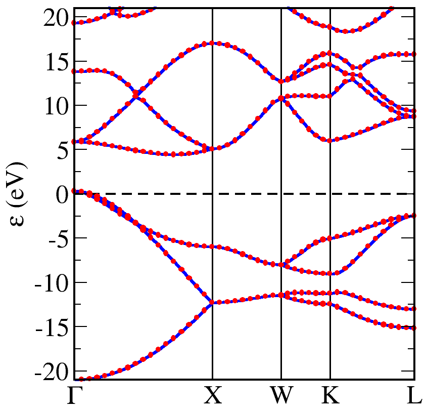
Appendix B Projected Density of States: LDA+ vs LXC-LDA+
The non-locality in LDA+ originates from the Hubbard- term[134, 135, 136]. By contrast, the LXC-LDA+, by its very nature must act on all orbitals in the same manner since it is a local (multiplicative) potential. The identification of the character of bands with regards to the angular momentum must thus be done with some care since it is not guaranteed that either method will preserve the character of bands that is obtained by the LDA.
We performed a series of LDA+ calculations with a Hubbard- applied to the transition metal cation’s orbitals before inverting these densities to find the LXC-LDA+ band structure. We calculated the projected density of states (PDOS) using the OptaDOS code[146] which implements the population analysis methodology of Segall et al.[148] to determine the character of each band by projecting the Kohn-Sham orbital onto a linear combination of atomic orbitals (LCAO) with the broadening scheme of Yates et al.[147] with a adaptive smearing ratio of 0.4. A Monkhorst-Pack k-point grid with a spacing of was used for the PDOS calculation. The PDOS is plotted alongside the associated band structure in Fig 17l for each transition metal monoxide (TMO) for the LDA, LDA+ and LXC-LDA+ methods at .
In general, one can see that the inversion largely preserves the PDOS as the Hubbard- parameter is varied and the only substantial significant change one observes is in the calculated gap where it appears that the eigenvalues are merely shifted by a largely constant amount. This behaviour also manifests itself in the insensitivity of the total band width bands with largely -character with increasing and in particular, similar to the LDA band width. This is not true however for the LDA+ where one sees that as is applied, additional bands start acquiring character and that the valence band and other occupied states near it start to show hybridisation of the transition metal cation’s electrons with the oxygen states.
Regarding material-specific differences, we point out that CoO has a larger difference in the LXC-LDA+ PDOS compared to MnO and NiO and as pointed out in the main text, also does not recover the dispersion of LDA to the same extent as in MnO and NiO. FeO proves once again to be somewhat of a special case amongst these class of materials where in the LDA case, almost all occupied bands shown have character and exhibit strong hybridisation with oxygen states, thus making it difficult to identify specific bands with character. This contrasts with the behaviour with the other TMOs where the highest occupied bands where is the total number of electrons also have predominantly -character. With LDA+, as we have previously stated, occupied bands near the valence band start to have oxygen -character; the difference in FeO however is much more stark to the extent that these bands have predominantly oxygen- character.
For calculations of the total band width for each TMO presented in the main text, we treated the LDA PDOS as a reference, obtaining the bands with pre-dominantly character. We then calculated the total band width for these set of bands for LDA+ and LXC-LDA+.