Graph Similarity Regularized Softmax for Semi-Supervised Node Classification

Abstract

Graph Neural Networks (GNNs) are powerful deep learning models designed for graph-structured data, demonstrating effectiveness across a wide range of applications. The softmax function is the most commonly used classifier for semi-supervised node classification. However, the softmax function lacks spatial information of the graph structure. In this paper, we propose a graph similarity regularized softmax for GNNs in semi-supervised node classification. By incorporating non-local total variation (TV) regularization into the softmax activation function, we can more effectively capture the spatial information inherent in graphs. The weights in the non-local gradient and divergence operators are determined based on the graph’s adjacency matrix. We apply the proposed method into the architecture of GCN and GraphSAGE, testing them on citation and webpage linking datasets, respectively. Numerical experiments demonstrate its good performance in node classification and generalization capabilities. These results indicate that the graph similarity regularized softmax is effective on both assortative and disassortative graphs.

Index Terms - Graph neural networks, Node classification, Regularization, Non-local total variation.

1 Introduction

Graph Neural Networks (GNNs) is a type of neural network specifically designed to operate on graph-structured data. GNNs have overcome the Euclidean data limitation inherent in traditional convolutional Neural Networks (CNNs), facilitating applications in domains like machine translation [1], recommendation systems [31], bioinformatics [6], and interactive simulations [2]. Semi-supervised node classification is a crucial task in GNNs which employ node features and edge information within graph data to accurately predict node labels, even when only a limited number of labeled nodes are available. Graphs used in node classification tasks can be categorized into assortative and disassortative graph [18, 19] based on node homophily [20]. Graphs with high node homophily are known as assortative graphs, where nodes with the same label tend to cluster together, such as citation networks. Conversely, disassortative graph are characterized by lower node homophily, where nodes with the same label are more likely to be distant from each other, such as webpage linking networks.

Recently, many variants of GNNs have been proposed and attracted increasing attention. Some of GNNs focus on the aggregation of neighbor information. One notable method is the Graph Convolutional Network (GCN) introduced by Kipf and Welling [14]. The core idea behind GCN is to define convolution operations on graphs to effectively learn representations by aggregating information from a node’s neighbors. GraphSAGE [9] introduced an innovative sampling strategy that allows the model to randomly sample a fixed number of neighboring nodes at each layer, and then aggregate information through predefined aggregation functions. The most discussed aggregation functions are mean aggregation and max pooling, both of which have achieved decent performances in node classification tasks. Additionally, common methods for addressing the issue of aggregating neighbor information can be broadly divided into strengthening effective neighbor determination and improving the way aggregating the feature weights. Chen et al. [3] proposed the Label-Aware GCN framework, which refines the graph structure by increasing positive ratio of neighbors. Wang et al. [29] integrated the high-order motif-structure information into feature aggregation. Liu et al. [16], to complement the original feature data, generated more samples in the local neighborhood via data augmentation. Graph Attention Networks (GAT) [28] leverage the attention mechanism to dynamically allocate weights to neighboring nodes based on their similarity, enabling effective information aggregation from distant neighbors across multiple hops. In [32], Zhang et al. further developed this idea by introducing a model with a mask aggregator, which performs a Hadamard product between the feature vector of each neighbor, supporting both node-level and feature-level attention.

Researchers have made numerous attempts to address the overfitting issues in GNNs. Tian et al. [26] employ stochastic transformation and data perturbations at both the node and edge structure levels to regularize the unlabeled and labeled data. Pei et al. [21] measure the saliency of each node from a global perspective, specifically the semantic similarities between each node and the graph representation, and then use the learned saliency distribution to regularize GNNs. Some researchers have explored regularization from the perspective of the loss function. Kejani et al. [12] propose a global loss function that integrates supervised and unsupervised information, and mitigates overfitting through manifold regularization applied to unsupervised loss. However, the model with a limitation on high-order neighbors. To fully exploit the structured information, Dornaika [5] further extend this method’s feasibility by integrating high-order neighbor feature propagation strategy into each GNN layer. In addition, Fu et al. utilize p-Laplacian matrix [7] and hypergraph p-Laplacian [8] to explore manifold structural information, thereby preserving local structural information while completing regularization tasks. However, most studies in the field are grounded in empirical experience, our work introduces a novel approach based on the variational method.

Most studies employ a single split of train/validation/test for each dataset to evaluate the accuracy in semi-supervised node classification. However, Oleksandr et al. [25] found that different data splits can lead to significantly different rankings of models. They highlight a major risk: models developed using a single split often perform well only with that specific split, failing to evaluate the model’s true generalization capabilities. To address this limitation, they proposed an assessment strategy based on averaging results over 100 random train/validation/test splits for each dataset and 20 random parameter initializations for each split. This approach provides a more accurate evalution of model generalization performance, avoiding the pitfall of selecting a model that overfits to a single fixed test set.

Total Variation (TV) regularization [23] is one of the most widely used methods in image processing, known for its outstanding performance in image restoration tasks. Recently, Fan et al. [10] proposed a framework that integrates traditional variational regularization method into CNNs for semantic image segmentation. In their work, the softmax activation function is reinterpreted as the minimizer of a variational problem, then spatial TV regularization can be effectively incorporated into CNNs via the softmax activation function. These regularized CNNs not only achieve superior segmentation results but also exhibits enhanced robustness to noise. Based on this work, the authors [11] further introduced non-local TV regularization to the softmax activation function to capture long range dependency information in CNNs. They presented a primal-dual hybrid gradient method for this proposed method. Numerical experiments show that this approach can eliminate isolated regions while preserving more details. Furthermore, instead of using TV regularization, Liu et al. [15] proposed a Soft Threshold Dynamics (STD) framework that can easily integrate various spatial priors, such as spatial regularity, volume constraints and star-shape priori, into CNNs for image segmentation. These methods combine the strengths of both CNNs and model-based methods by applying a variational perspective to the softmax activation function.

Inspired by these works, we aim to apply this variational regularization method to GNNs for node classification tasks, incorporating the non-local TV regularization into the softmax activation function. It can help GNNs to better capture the spatial information inherent in graphs. Unlike CNNs, where the similarity relationship between data points must be carefully determined, GNNs inherently provide this relationship through the adjacent matrix. We apply the proposed method into the architecture of GCN and GraphSAGE, testing them on citation and webpage linking datasets, respectively. Numerical experiments demonstrate that this variational regularization method is also well-suited for GNNs, and exhibits strong generalization capabilities across 100 random dataset splits and 20 random parameter initializations for each split. The contributions of this paper can be summarized as follows:

• We introduce a novel graph similarity regularized softmax for GNNs in semi-supervised node classification.

• We propose a framework for integrating the traditional variational regularization method into GNNs.

The article is structured as follows: In Section II, we provide a concise overview of related work, including GCN, GraphSAGE and softmax variational problem. Section III presents the regularized GNNs model and algorithm. Experimental results and implementation details are reported in Section IV. We conclude this paper in Section V.

2 Related Work

For a graph $\mathcal{G}=\{\mathcal{V},\mathcal{E}\}$, where $\mathcal{V}$ and $\mathcal{E}$ represent the set of nodes and edges, respectively. Let $N$ denote the number of nodes, and let $d$ represent the number of features for each node. A node $x_{i}\in\mathcal{V}$ has a neighborhood $\mathcal{N}(x_{i})=\{x_{j}\in\mathcal{V}|(x_{i},x_{j})\in\mathcal{E}\}$, where $(x_{i},x_{j})$ represents an edge between nodes $x_{i}$ and $x_{j}$. The adjacency matrix $A$ is an $N\times N$ matrix with $A_{ij}=1$ if $(x_{i},x_{j})\in\mathcal{E}$ and $A_{ij}=0$ otherwise. The feature matrix $X\in\mathbb{R}^{N\times d}$ represents the features of the nodes, and the nodes are characterized by $K$ classification labels.

In this section, we first introduce the general form of GNNs and the discuss two special instances: GCN and GraphSAGE. In addition, we give the variational form of softmax function, which lays the foundation for next section.

2.1 Graph Neural Networks

The fundamental idea of GNNs is to iteratively update the representation of each node by combing both its own features and the features of its neighboring nodes. In [30], Xu et al. proposed a general framework for GNNs, where each layer consists two important functions as follows:

• AGGREGATE function: This function aggregates information from the neighboring nodes of each node.

• COMBINE function: This function updates the node’s representation by combining the aggregated information from its neighbors with its current representation.

Mathematically, the $l$-th layer of a GNN can be defined as follows:

$$\begin{gathered}a_{i}^{(l)}=\text{AGGREGATE}^{(l)}(\{H_{j}^{(l-1)}:x_{j}\in\mathcal{N}(x_{i})\}),\\ i=1,2,...,N,\end{gathered}$$ (1)

$$H_{i}^{(l)}=\text{COMBINE}^{(l)}(H_{i}^{(l-1)},a^{(l)}_{i}),i=1,2,...,N,$$ (2)

where $H^{(l)}$ represents the feature matrix at the $l$-th layer (with $H^{(0)}=X$ being the input feature matrix), and $a_{i}^{(l)}$ denotes the aggregated feature vector of node $x_{i}$ at the $l$-th layer. Different GNNs employ various AGGREGATE and COMBINE functions [30, 14, 28, 9]. The node representations in the final layer $H^{(L)}$ can be considered the final representations of the nodes, denoted as $H^{(L)}=\text{GNN}(X)\in\mathbb{R}^{N\times D}$, then it can be used for node label prediction through the softmax function:

$$\hat{Y}=\text{softmax}(H^{(L)}W).$$ (3)

where $W\in\mathbb{R}^{D\times K}$ is a learnable matrix.

2.2 Graph Convolutional Network

In [14], Kipf and Welling proposed a classical GCN. Each layer of GCN can be defined as follows:

$$H^{(l+1)}=\sigma(\tilde{D}^{-\frac{1}{2}}\tilde{A}\tilde{D}^{-\frac{1}{2}}H^{(l)}W^{(l)}),$$ (4)

where $\tilde{A}=A+I_{N}\in\mathbb{R}^{N\times N}$ is the adjacency matrix of the graph with added self-connections (where $I_{N}$ is the identity matrix of size $N$), $\tilde{D}$ is the degree matrix of $\tilde{A}$, $W^{(l)}$ is the layer-specific trainable weight matrix, and $\sigma$ is an activation function, such as ReLU and softmax.

Commonly the feature matrix $X$ and adjacency matrix $A$ of the entire graph are input through a two-layer GCN, defined as follows:

$$\hat{Y}=\text{softmax}(\hat{A}\text{ReLU}(\hat{A}XW^{(0)})W^{(1)}),$$ (5)

where $\hat{A}=\tilde{D}^{-\frac{1}{2}}\tilde{A}\tilde{D}^{-\frac{1}{2}}\in\mathbb{R}^{N\times N}$ is the normalized adjacency matrix with added self-connections, $W^{(0)}$ and $W^{(1)}$ are the trainable weight matrices of the first and second layers, respectively, and $\hat{Y}\in\mathbb{R}^{N\times K}$ represents the output of this network.

GCN is trained by minimizing a cross-entropy loss function, which aims to make the predicted labels of nodes in the training set as close as possible to their ground truth labels. This loss function is commonly used for classification problems and is given by

$$L(Y,\hat{Y})=-\sum_{i\in\mathcal{Y}_{L}}\sum^{K}_{k=1}Y_{ik}\text{ln}\hat{Y}_{ik},$$ (6)

where $\mathcal{Y}_{L}$ is the set of indexes for the nodes used for training. $Y_{i}$ represents the ground-truth probability distribution of the $i$-th node, which is represented as a one-hot vector, with $Y_{ik}$ indicating whether the $i$-th node belongs to the $k$-th class. $\hat{Y}_{ik}$ represents the predicted probability of the $i$-th node belonging to class $k$.

2.3 GraphSAGE

In [9], Hamilton et al. introduced a groundbreaking graph neural network model known as GraphSAGE. During each iteration, a fixed number of neighboring nodes are sampled for each central node, and these nodes are then aggregated as formulated in (1). There are three alternative AGGREGATION functions available:

• Mean Aggregator: Computes the average of the neighbor embeddings, which is combined with the central node’s embedding through a non-linear trasformation.

• LSTM Aggregator: Utilizes Long Short-Term Memory (LSTM) networks to process a sequence of neighbor embeddings. It is important to randomize the order of neighbors to ensure the model does not rely on a specific sequence, as graph structures are inherently unordered.

• Pooling Aggregator: Applies non-linear transformation followed by pooling operations, such as max or average pooling to the neighbor embeddings to extract the most significant features.

Subsequently, the aggregated information is combined with the state of the central node, as depicted in (2). This COMBINE function is specifically defined by the following formula:

$$H_{i}^{(l)}=\sigma(W^{(l)}\cdot\text{CONCAT}(H_{i}^{(l-1)},a_{i}^{(l)})).$$ (7)

where CONCAT denotes the concatenation operation and $W^{(l)}$ is the weight matrix at layer $l$. By choosing an appropriate aggregation function and training the model with the loss function (6), GraphSAGE can effectively learn node embeddings that generalize well to unseen nodes, making it a powerful tool for inductive learning on graphs.

2.4 Softmax Variational Problem

The softmax function is most commonly used in the last layer of neural networks for classification tasks. It converts the input logits into a probability distribution, facilitating the identification of the class with the highest probability as the predicted class. In [11], Liu et al. provide a variational interpretation of the softmax function, showing that it can be derived from the following minimization problem:

$$\begin{gathered}\min_{\mathscr{A}}-\langle\mathscr{A},O\rangle+\epsilon\langle\mathscr{A},\log\mathscr{A}\rangle,\\ \text{s.t.}\sum_{k=1}^{K}\mathscr{A}_{ik}=1,\mathscr{A}_{ik}\geq 0,\forall i=1,2,...,N,\end{gathered}$$ (8)

where $O=(O_{1},O_{2},...,O_{K})\in\mathbb{R}^{N\times K}$ is the given input, $\mathscr{A}=(\mathscr{A}_{1},\mathscr{A}_{2},...,\mathscr{A}_{K})\in\mathbb{R}^{N\times K}$ is the output we aim to find, the second term of the objective function can be interpreted as a negative entropy term. This term enforces smoothness on $\mathscr{A}$ with a positive control parameter $\epsilon>0$. The equation represents the constraint condition that the sum of each row of $\mathscr{A}$ is 1. Using the Lagrange method, the minimizer of the above problem is:

$$\mathscr{A}^{*}_{ik}=\frac{\exp\frac{O_{ik}}{\epsilon}}{\sum^{K}_{\hat{k}=1}\exp\frac{O_{i\hat{k}}}{\epsilon}},$$ (9)

where $O_{ik}$ represents the probability of the $i$-th node belonging to the $k$-th class. This can be equivalently reformulated in matrix form as

$$\mathscr{A^{*}}=\text{softmax}\left(\frac{O}{\epsilon}\right).$$ (10)

In fact, when $\epsilon=1$, it is exactly the softmax activation function, i.e.,

$$\mathscr{A^{*}}=\text{softmax}(O).$$ (11)

3 Methods and Algorithms

3.1 The Non-local TV Regularized Softmax Function

Considering that the softmax activation function does not have any spatial regularization, Liu et al. [11] proposed a novel regularized softmax activation function by integrating non-local TV regularization, defined as follows:

$$\begin{gathered}\min_{\mathscr{A}}{\sum_{k=1}^{K}\{-\langle\mathscr{A}_{k},O_{k}\rangle+\epsilon\langle\mathscr{A}_{k},\log\mathscr{A}_{k}\rangle+\lambda NLTV(\mathscr{A}_{k})}\}\\ \text{s.t.}\sum_{k=1}^{K}\mathscr{A}_{ik}=1,\forall i=1,2,...,N,\end{gathered}$$ (12)

where $\lambda$ is a regularization parameter, and the variational formulation of non-local TV is given in the following form

$$NLTV(\mathscr{A}_{k})=\max_{\|\eta_{k}\|_{\infty}\leqslant 1}\left\langle\mathscr{A}_{k},\operatorname{div}_{\textbf{S}}\eta_{k}\right\rangle,$$ (13)

where $\eta_{k}\in\mathbb{R}^{N\times N}$ is the dual variable associated with $\mathscr{A}_{k}$, $\eta_{k}(j)$ denotes the $j$-th row of $\eta_{k}$, and the infinity norm $\|\eta_{k}\|_{\infty}=\max\limits_{j}\|\eta_{k}(j)\|_{2}$ represents the maximum Euclidean norm among all the rows of the matrix $\eta_{k}$. By substituting the above equation, the minimization problem (12) is equivalently reformulated as the following min-max problem:

$$\begin{gathered}\min_{\mathscr{A}}\max_{\|\eta_{k}\|_{\infty}\leqslant 1}\sum_{k=1}^{K}\{-\langle\mathscr{A}_{k},O_{k}\rangle+\epsilon\langle\mathscr{A}_{k},\log\mathscr{A}_{k}\rangle\\ +\lambda\left\langle\mathscr{A}_{k},\operatorname{div}_{\textbf{S}}\eta_{k}\right\rangle\},\\ \text{s.t.}\sum_{k=1}^{K}\mathscr{A}_{ik}=1,\forall i=1,2,...,N.\end{gathered}$$ (14)

By employing the alternating minimization algorithm to solve this problem, it can be decomposed into two subproblems for $\eta$ and $\mathscr{A}$ respectively:

• $\eta$-subproblem:

  For fixed $\mathscr{A}$, we solve

  $$\max_{\|\eta_{k}\|_{\infty}\leqslant 1}\left\langle\mathscr{A}_{k},\operatorname{div}_{\textbf{S}}\eta_{k}\right\rangle.$$ (15)

• $\mathscr{A}$-subproblem:

  For fixed $\eta$, we solve

  $$\begin{gathered}\min_{\mathscr{A}}\sum_{k=1}^{K}\{-\langle\mathscr{A}_{k},O_{k}\rangle+\epsilon\langle\mathscr{A}_{k},\log\mathscr{A}_{k}\rangle+\lambda\left\langle\mathscr{A}_{k},\operatorname{div}_{\textbf{S}}\eta_{k}\right\rangle\}\\ \text{s.t.}\sum_{k=1}^{K}\mathscr{A}_{ik}=1.\end{gathered}$$ (16)

For the $\eta$-subproblem, it is solved using the Lagrange multiplier technique, while for the $\mathscr{A}$-subproblem, it is tackled through gradient descent combined with a projection operator. More detailed information on solving these two subproblems can be found in Appendix (Calculating the $\mathscr{A}$-subproblem and $\eta$-subproblem in RGNN). Then, the iteration can be expressed as:

$$\begin{cases}\begin{aligned} \eta^{t}_{k}&=\mathcal{P}_{B}\left(\eta^{t-1}_{k}-\tau\nabla_{\textbf{S}}\mathscr{A}_{k}^{t-1}\right),\\ \mathscr{A}^{t}_{k}&=\operatorname{softmax}\left(\frac{O_{k}-\lambda\operatorname{div}_{\textbf{S}}\eta^{t}_{k}}{\epsilon}\right),\end{aligned}\end{cases}k=1,2,...,K,$$ (17)

where $\bigtriangledown_{\textbf{S}}\mathscr{A}_{k}\in\mathbb{R}^{N\times N}$ and $\operatorname{div}_{\textbf{S}}\eta_{k}\in\mathbb{R}^{N}$ represent the non-local gradient operator and non-local divergence operator, respectively.

The non-local gradient operator ${\bigtriangledown}_{\textbf{S}}u(x):L^{2}(\mathcal{V})\rightarrow L^{2}(\mathcal{V}\times\mathcal{V})$ is defined as

$$({\bigtriangledown}_{\textbf{S}}u)(x_{i},x_{j})=\textbf{S}(x_{i},x_{j})(u(x_{j})-u(x_{i})),i=1,2,...,N.$$ (18)

The non-local divergence operator $\operatorname{div}_{\textbf{S}}v(x):L^{2}(\mathcal{V}\times\mathcal{V})\rightarrow L^{2}(\mathcal{V})$ is defined as

$$\begin{gathered}(\operatorname{div}_{\textbf{S}}v)(x_{i})=\sum_{x_{j}\in\mathcal{N}(x_{i})}\textbf{S}(x_{i},x_{j})(v(x_{i},x_{j})-v(x_{j},x_{i})),\\ i=1,2,...,N.\end{gathered}$$ (19)

Here, $\textbf{S}(x_{i},x_{j})\geq 0$ is the weight function that measures the similarity between two nodes $x_{i}$ and $x_{j}$. In [11], Liu et al. provide several methods to define a proper weight function to depict the relationship between data points, which are crucial for grid-structured data like images. However, for graph-structured data, the relationship between nodes have already been directly given in the form of adjacency matrix $A$. To ensure stable training, we use the normalized form to define the similarity matrix $\textbf{S}=D^{-\frac{1}{2}}AD^{-\frac{1}{2}}$, with $D$ being the diagonal degree matrix of $A$.

The projection operator is given by

$$\mathcal{P}_{B}(\eta_{k})=\begin{cases}\begin{aligned} &\eta_{k}(j),&\left\|\eta_{k}(j)\right\|_{2}\leq 1,\\ &\frac{\eta_{k}(j)}{\left\|\eta_{k}\right\|_{\infty}},&\left\|\eta_{k}(j)\right\|_{2}>1,\end{aligned}\end{cases}$$ (20)

where $\eta_{k}(j)\in\mathbb{R}^{N}$ denotes the $j$-th row of $\eta_{k}$ and $\|\eta_{k}\|_{\infty}=\max\limits_{j}\|\eta_{k}(j)\|_{2}$.

Therefore, the non-local TV regularized softmax function can be expressed as:

$$\mathscr{A}^{*}=\operatorname{softmax}\left(\frac{O-\lambda\operatorname{div}_{\textbf{S}}\eta}{\epsilon}\right).$$ (21)

3.2 The Proposed RGNN Algorithm

In this section, we propose to apply the regularized non-local TV softmax function within the GNN framework. In the forward process, we first initialize the learnable weight matrices $W^{(l)},l=1,...,L$ in the GNN models. For each epoch, we then initialize $\mathscr{A}^{0}$ as follows:

$$\mathscr{A}^{0}=\text{softmax}(O),$$ (22)

where $O=\text{GNN}(X)\in\mathbb{R}^{N\times K}$ represents the output node features of the GNN before applying the softmax function. Here, $\mathscr{A}^{0}$ corresponds to the output classes generated by the forward process of traditional GNN models. Based on these results and setting $\eta^{(0)}=\textbf{0}$, we proceed to compute the following iterations to update $\eta$ and $\mathscr{A}$ for the non-local TV regularized softmax function:

• $\eta$-subproblem:

  Step 1. Compute the non-local gradient operator:
  

  $$\begin{gathered}(\bigtriangledown_{\textbf{S}}\mathscr{A}^{t-1}_{k})(x_{i},x_{j})=\textbf{S}(x_{i},x_{j})(\mathscr{A}^{t-1}_{jk}-\mathscr{A}^{t-1}_{ik}),\\ i,j=1,2,...,N,k=1,2,...,K,\end{gathered}$$ (23)

  where the similarity matrix $\textbf{S}=D^{-\frac{1}{2}}AD^{-\frac{1}{2}}$. In the context of the graph structure, the selection of S is linked to the adjacency matrix $A$ of the given graph.

  Step 2. Update $\eta_{k}$ using the gradient descent method and the projection operator:

  $$\eta_{k}^{t}=\mathcal{P}_{B}(\eta^{t-1}_{k}-\tau\bigtriangledown_{\textbf{S}}\mathscr{A}^{t-1}_{k}),k=1,2,...,K.\\$$ (24)

• $\mathscr{A}$-subproblem:

  Step 1. Compute the non-local divergence operator:

  $$\begin{gathered}(\operatorname{div}_{\textbf{S}}\eta^{t}_{k})(x_{i})=\sum_{x_{j}\in\mathcal{N}(x_{i})}\textbf{S}(x_{i},x_{j})(\eta^{t}_{k}(x_{i},x_{j})\\ -\eta^{t}_{k}(x_{j},x_{i})),\\ i=1,2,...,N,k=1,2,...,K.\end{gathered}$$ (25)

  Step 2. Calculate the non-local TV regularized softmax function:

  $$\mathscr{A}^{t}_{k}=\text{softmax}\left(\frac{O_{k}-\lambda\operatorname{div}_{\textbf{S}}\eta^{t}_{k}}{\epsilon}\right),k=1,2,...,K.$$ (26)

After iterating to obtain the optimal matrix $\hat{Y}=\mathscr{A}^{T}$, we proceed to compute the cross-entropy loss $L(\hat{Y},Y)$ between $\hat{Y}$ and the ground-truth probability distribution matrix $Y$. In the backward process, we compute the gradient of the loss $L$ with respect the parameters $W^{(l)}$ using automatic differentiation. This process traverses the computational graph backward and is commonly implemented in machine learning frameworks. This gradient $\frac{\partial L}{\partial W^{(l)}}$ is then used in popular optimizers like stochastic gradient descent (SGD) [22] or its variants to update the parameters $W^{(l)}$ during training.

We summarize the proposed RGNN algorithm in Algorithm 1. To better understanding, Figure 1 illustrates the differences between the structures of GNN and RGNN.

Input: Graph $\mathcal{G}(\mathcal{V},\mathcal{E})$, feature matrix $X$, learnable parameters $\lambda,\epsilon,\tau$, external iterations number $M$ and internal iterations number $T$.

1

2Initialize: $W^{(l)},l=1,2,...,L$.

3 for $epoch=1,2,...,M$ do

4       $O=\text{GNN}(X)$, $\mathscr{A}^{0}=\text{softmax}(O)$,

5       Set $\eta^{0}=\textbf{0}$.

6       for $t=1,2,...,T$ do

7             $\eta$-subproblem:

8               (1)compute the non-local gradient operator $\bigtriangledown_{\textbf{S}}\mathscr{A}^{t-1}$ by (23).

9               (2)update $\eta^{t}$ using gradient descent and projection operator by (24).

10            

11            $\mathscr{A}$-subproblem:

12               (1)compute the non-local divergence operator $\operatorname{div}_{\textbf{S}}\eta^{t}$ by (25).

13               (2)calculate the regularized softmax function $\mathscr{A}^{t}$ by (26).

14       end for

15      Get the matrix $\hat{Y}=\mathscr{A}^{T}$ and compute the cross-entropy function $L(Y,\hat{Y})$.

16       Update $W^{(l)}$ by using gradient descent method.

17 end for

Output: $W^{(l)},l=1,2,..,L$.

Algorithm 1 RGNN algorithm

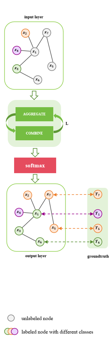
(a) original GNN

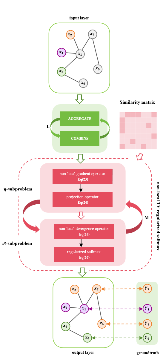
(b) RGNN

Figure 1: GNN vs. RGNN: A structural comparison. (The output shows that node $x_{1}$ is misclassified by the GNN but correctly classified by the RGNN.)

4 Experiments

4.1 Datasets

In this paper, we discuss the performance of our proposed RGNN approach on both assortative and disassortative datasets.

4.1.1 Assortative datasets

We utilize three standard citation network benchmark datasets for the semi-supervised node classification task: Cora, Citeseer, and Pubmed [24, 17]. In these datasets, nodes represent individual documents, while edges represent citation relationships between these documents. Node features are extracted from the bag-of-words representation of the document content, and each node is associate with a corresponding class label.

4.1.2 Disassortative datasets

We employ three specialized webpage linking network benchmark datasets: Cornell, Texas, Wisconsin, which are subdatasets of WebKB [4], collected from computer science departments of various universities. In these datasets, nodes represent web pages and edges are hyperlinks between them. Node features are bag-of-words representation of web pages.

We provide the statistics of each dataset in Table 1.

Table 1: Graph Dataset Statistics.

	Assortative			Disassortative
Datasets	Cora	Citeseer	Pubmed	Cornell	Texas	Wisconsin
Classes	7	6	3	5	5	5
Features	1433	3703	500	1703	1703	1703
Nodes	2485	2120	19717	183	183	251
Edges	5069	3679	44324	295	309	499

4.2 Parameters initialization

All experiments are conducted using PyTorch on an NVIDIA RTX 3090 GPU with 24GB of memory. We train our proposed RGNN models for a maximum of 10000 epochs, with early stopping implemented if the validation loss does not decrease or the accuracy does not increase for 50 consecutive epochs. All the network parameters are initialized using Glorot initialization and optimized using the Adam optimizer [13].

Since the optimal hyperparameters may vary across different random splits and initializations, we treat these three hyperparameters $\tau$, $\lambda$ and $\epsilon$ in the proposed RGNN model as learnable, starting with initial values. Table 2 outlines our parameters initialization and learning rate. To optimize computation time, our experiments generally focus on the case where $T=1$. Despite this limitation, this regularized softmax approach still proves effective in our numerical experiments.

Table 2: Initial values and learning rate (Lr) of parameters for RGNN.

	Cor.	Cit.	Pub.	Cor.	Tex.	Wis.	Lr
$\tau_{ini}$	1.0	0.3	1.0	0.01	0.01	0.01	0.01
$\lambda_{ini}$	3.0	8.0	3.0	0.3	3.0	1.0	0.001
$\epsilon_{ini}$	1.0	5.0	0.5	8.0	3.0	1.0	0.01

4.3 Experimental Results

In this section, we conduct a thorough comparison of our proposed RGNN method with several prominent graph learning approaches: GCN [14], GAT [28], and two variants of GraphSAGE (mean and maxpool) [9]. We evaluate the average classification performance of each method across 2000 experiments, with 100 random dataset splits and 20 random initializations.

4.3.1 Experiments on assortative datasets

Recognizing the superior performance of GCN on assortative datasets-Cora, Citeseer, and Pubmed-we integrate the non-local TV regularized softmax into GCN, resulting in the regularized GCN (RGCN). We compare the performance of RGCN with standard GCN, GAT and GraphSAGE-mean and GraphSAGE-maxpool. For each dataset split, the training set is formed by randomly selecting 20 nodes per class, the validation set by selecting 30 nodes per class, with the remainder assigned to the test set. The results, presented in Table 3, indicate that the RGCN model outperforms the standard GCN and consistently achieves the highest average accuracy across all these three citation datasets. This highlights the efficiency of the softmax regularization and its robust generalization capabilities.

Table 3: The mean accuracy and std (%) over 100 random dataset splits and 20 random initializations for each split.

	Cora	Citeseer	Pubmed
GCN [14]	81.5±1.3	72.1±1.6	79.0±2.1
GAT [28]	80.8±1.3	71.6±1.7	78.6±2.1
GraphSAGE-mean [9]	79.3±1.3	71.6±1.6	76.1±2.0
GraphSAGE-maxpool [9]	76.7±1.8	67.4±2.2	76.9±2.0
RGCN(ours)	81.9±1.1	74.1±1.6	79.2±2.1

4.3.2 Experiments on disassortative datasets

Considering GraphSAGE’s proficiency with disassortative datasets, we integrate the non-local TV regularized softmax into GraphSAGE-mean, resulting in RGraphSAGE-mean. We compare its performance with standard GraphSAGE-mean, GraphSAGE-maxpool, GCN, and GAT on Cornell, Texas, and Wisconsin datasets. Due to the small number of nodes in some classes, we modified the partitioning strategy for dataset splits, randomly allocating 60%, 20%, and 20% of the nodes to the training, validation, and test sets, respectively. Table 4 demonstrates that RGraphSAGE-mean significantly outperforms GraphSAGE-mean and other test methods across these webpage datasets, underscoring its practical efficacy of non-local TV regularized softmax. Additionally, these average results over 2000 experiments suggest that our regularized model maintains robust performance across different dataset splits and initializations.

Table 4: The mean accuracy and std (%) over 100 random dataset splits and 20 random initializations for each split.

	Cornell	Texas	Wisconsin
GCN [14]	36.7±3.9	42.4±3.3	51.8±3.3
GAT [28]	41.2±3.3	46.8±5.0	51.8±4.2
GraphSAGE-mean [9]	76.4±6.0	78.6±4.1	78.7±2.1
GraphSAGE-maxpool [9]	66.6±5.8	77.5±4.2	74.0±1.6
RGraphSAGE-mean(ours)	80.8±6.4	81.4±6.2	80.8±5.7

4.4 Further Discussion

4.4.1 Comparison of time consumption

By incorporating the non-local TV regularized softmax into GNNs, addition computation is required compared to original GNNs, which can increase training time. Table 5 and Table 6 provide a comparison of time expenditure for RGCN, RGraphSAGE-mean and their counterparts during a single training epoch. It can be observed that the training time has a certain increase compare to GCN and GraphSAGE. However, this additional computational cost can lead to significant improvement in model accuracy and generalization.

Table 5: Time(s) per epoch for different GNNs on citation datasets.

	Cora	Citeseer	Pubmed
GCN [14]	3.55e-3	3.72e-3	3.69e-3
GAT [28]	8.78e-3	8.97e-3	1.53e-2
GraphSAGE-mean [9]	4.69e-3	4.34e-3	5.10e-3
GraphSAGE-maxpool [9]	4.45e-3	6.05e-3	8.16e-3
RGCN(ours)	2.98e-3	2.87e-2	2.71e-1

Table 6: Time(s) per epoch for different GNNs on webpage datasets.

	Cornell	Texas	Wisconsin
GCN [14]	3.41e-3	3.51e-3	3.64e-3
GAT [28]	8.72e-3	8.13e-3	8.50e-3
GraphSAGE-mean [9]	4.65e-3	4.59e-3	4.74e-3
GraphSAGE-maxpool [9]	2.79e-3	2.85e-3	2.96e-3
RGraphSAGE-mean(ours)	4.05e-2	3.85e-2	3.79e-2

4.4.2 Parameters analysis

In this section, we discuss the performance of the RGCN model with different initializations for the three parameters $\tau$, $\lambda$, and $\epsilon$. Specifically, $\tau$ serves as the learning rate for the gradient descent in the $\eta$-subproblem, $\lambda$ acts as the coefficient for the non-local TV regularization term, and $\epsilon$ represents the coefficient for the negative entropy term in the RGCN model.

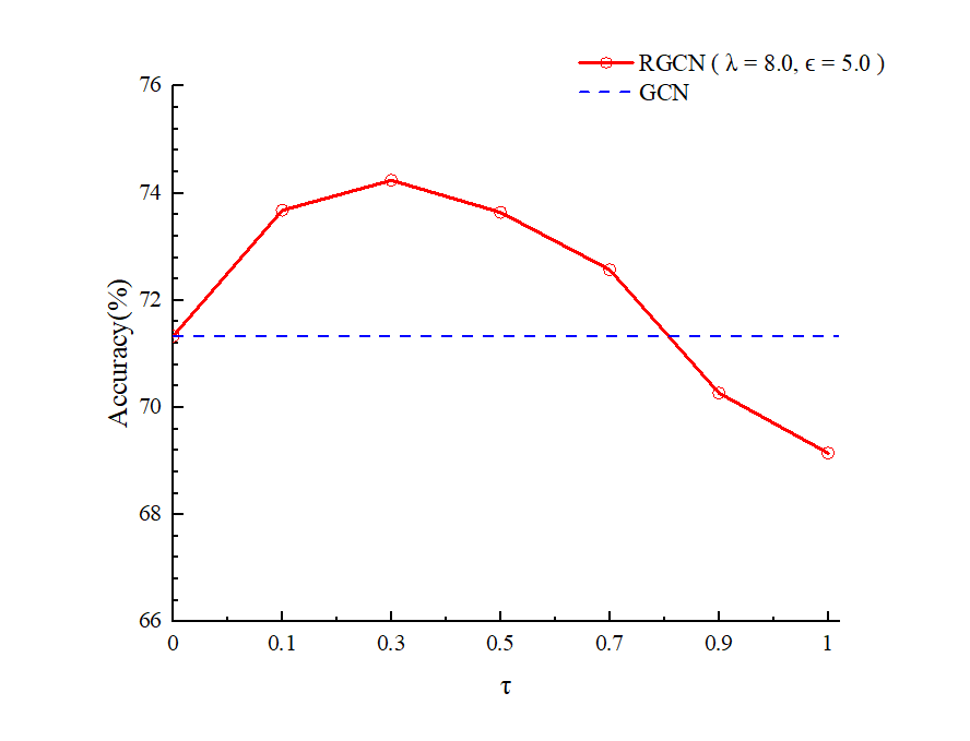
(a) $\tau$

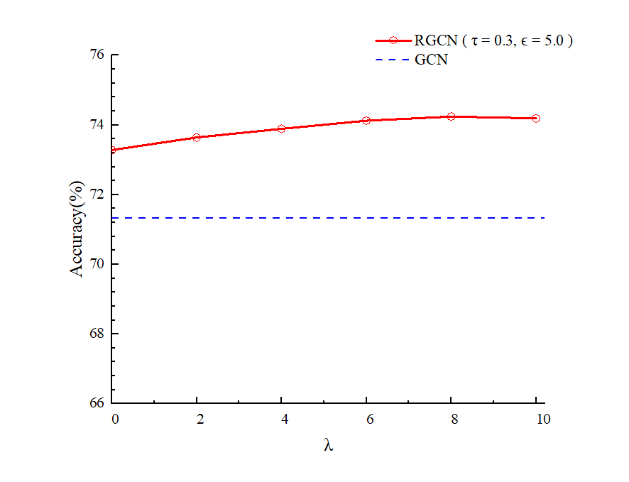
(b) $\lambda$

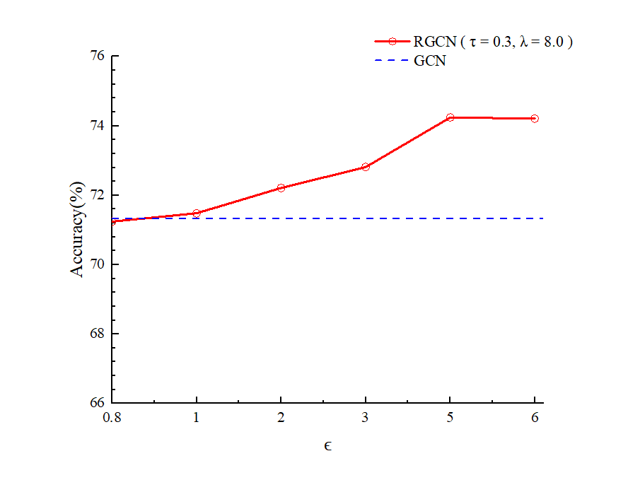
(c) $\epsilon$

Figure 2: Classification accuracy on Citeseer dataset of the RGCN model with varying initial settings of parameters $\tau$,$\lambda$ and $\epsilon$, respectively.

In Figure 2, we evaluate the influence of each hyperparameter by keeping the initial values of the other two hyperparameters fixed. The average classification accuracy are obtained from 5 random data splits and 5 random parameter initializations on Citeseer dataset. We observe that when the initial parameter values are within a certain range, the proposed RGCN model (represented by the red solid line) can consistently outperforms the baseline GCN model (indicated by the blue dashed line), highlighting the advantages of this non-local TV regularized softmax in GCN for semi-supervised node classification.

In Figure 2(a), with initial values set to $\lambda=8.0$ and $\epsilon=5.0$, it is evident that within the range of $(0,0.7]$ for parameter $\tau$, the RGCN model achieves superior accuracy compared to the standard GCN model, reaching its highest accuracy at $\tau=0.3$. In addition, we discuss the parameter $\lambda$ within $[0,10]$ with initial values set to $\epsilon=5.0$ and $\tau=0.3$. As depicted in Figure 2(b), experimental results of RGCN consistently outperform the GCN within this range, with the best performance achieved at $\lambda=8.0$. Similarly, the parameter $\epsilon$ is also very important for the experimental results shown in Figure 2(c), where the highest accuracy is achieved at $\epsilon=5.0$.

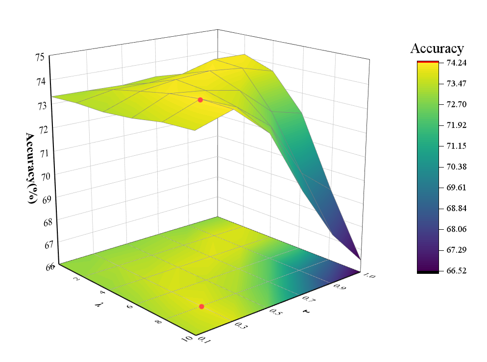
Figure 3: The combined impact of the scaling factor $\tau$ and regularization parameter $\lambda$ on Citeseer dataset.

Furthermore, we conducted an in-depth study on how the parameter $\tau$ and $\lambda$ collectively influence performance of RGCN on the Citeseer dataset, with the initial value of $\epsilon=5.0$. As depicted in Figure 3, when the initial value of $\tau$ approaches $1.0$, the model tends to perform poorly, especially as $\lambda$ also increases. Conversely, when the initial value of $\tau$ is closer to $0.1$, the model is more likely to exhibit superior performance. This indicates a significant correlation between these two parameters, with the optimal combination being $(\tau,\lambda)=(0.3,8.0)$, achieving the highest accuracy of $74.24\%$, as shown in Figure 3. Additionally, Figure 2(c) highlights that the intial value of $\epsilon$ is crucial for the performance of the RGNN model when $\tau$ and $\lambda$ are set to 0.3 and 8.0, respectively. These results indicate that the careful tuning of these three hyperparameters is essential for optimizing model performance, and proper combination of $\tau$, $\lambda$, and $\epsilon$ will enable the proposed RGNN model to achieve its best performance.

4.4.3 Visualization

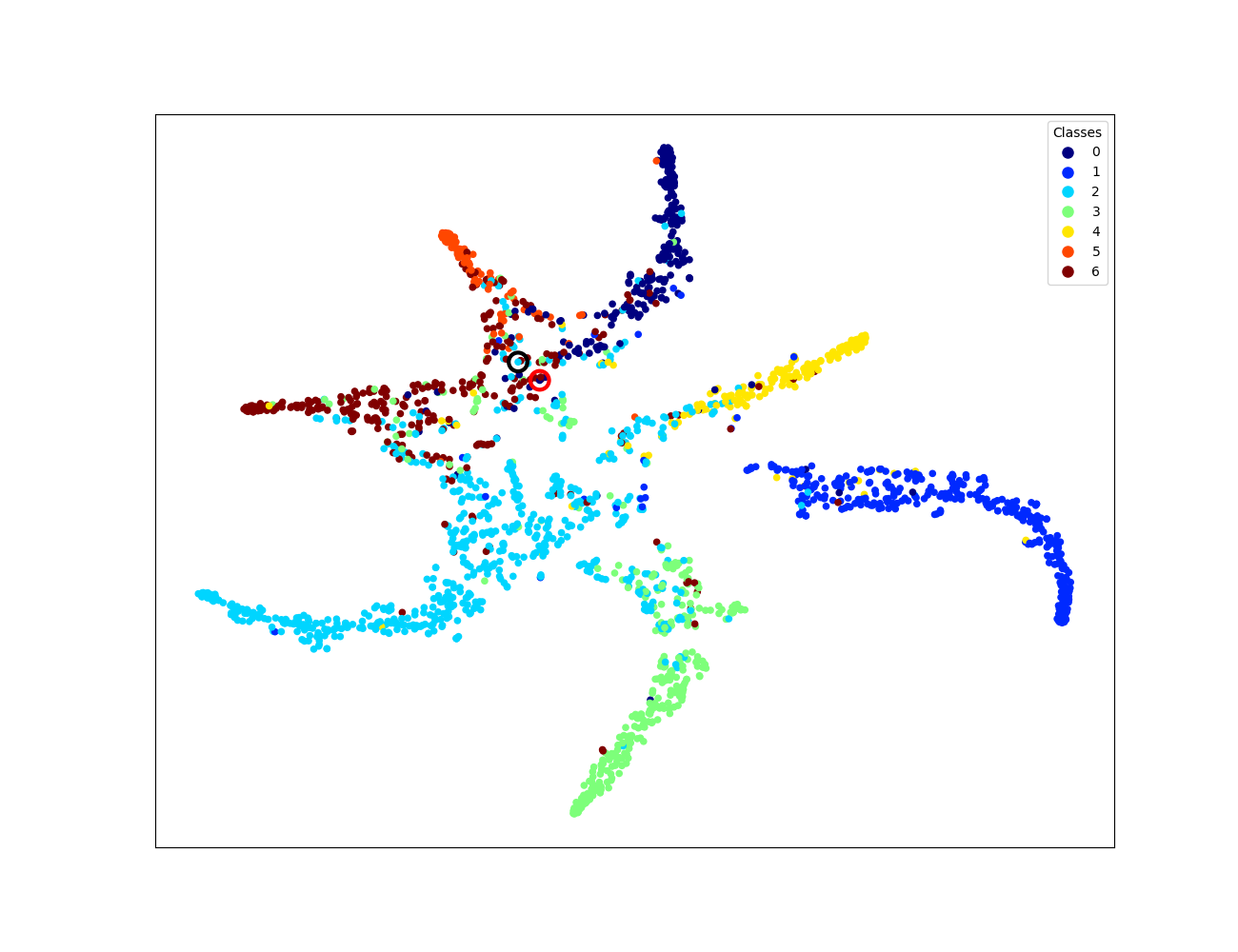
(a)

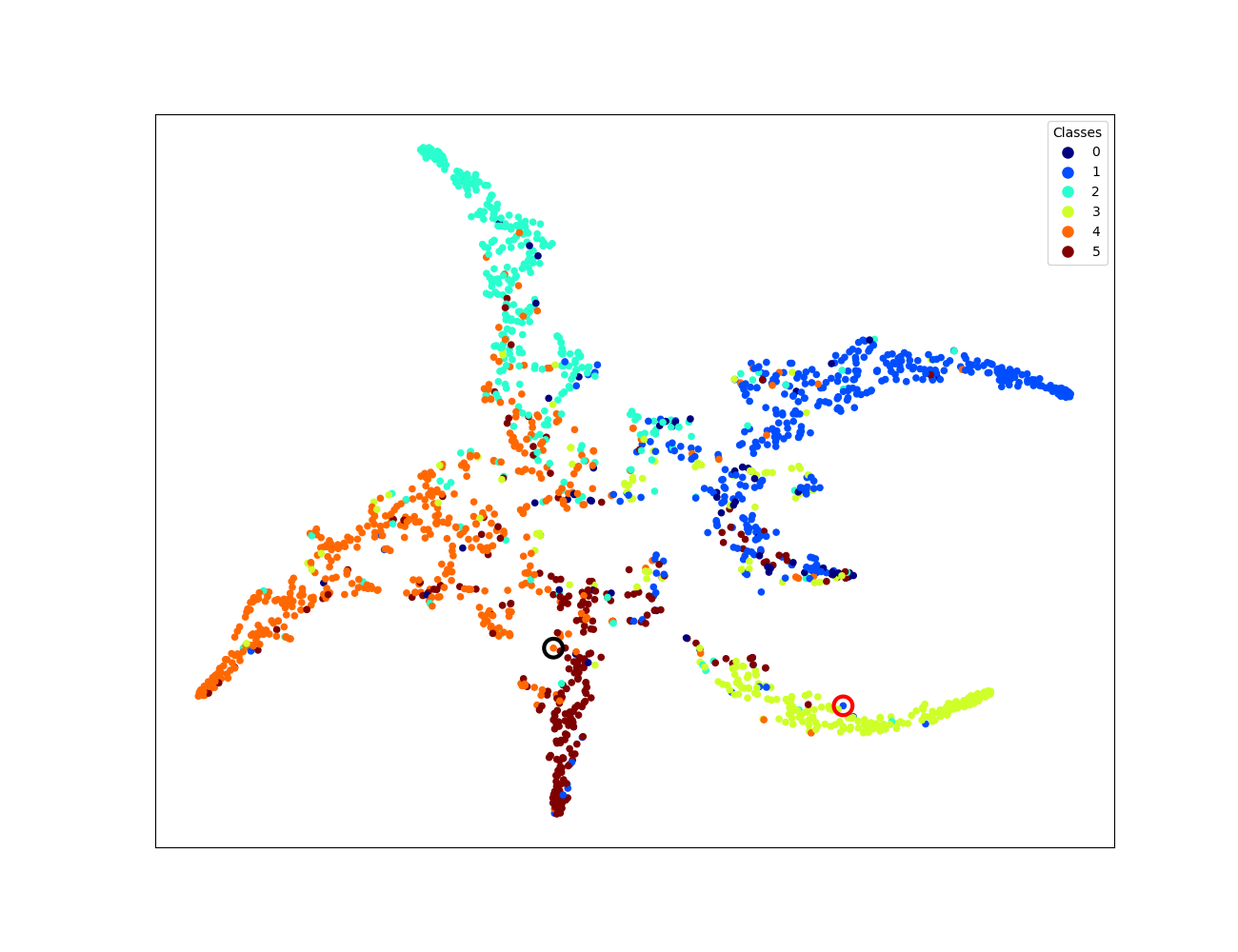
(a) GCN

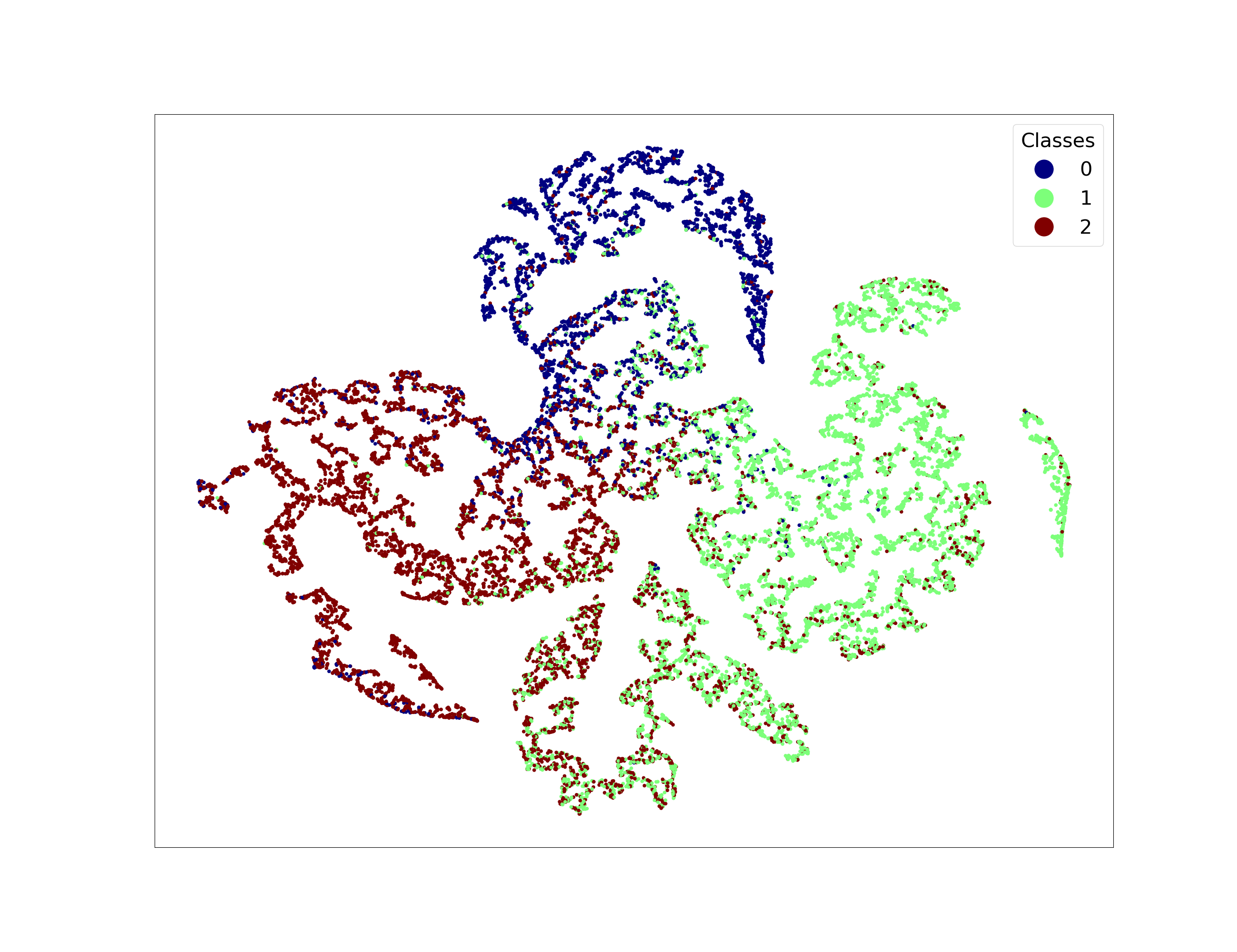
(b)

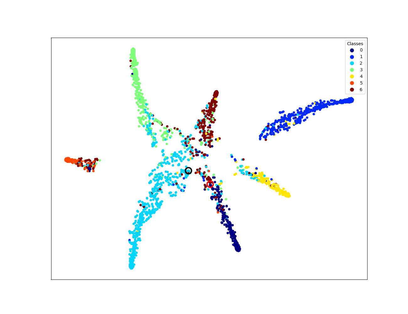
(c)

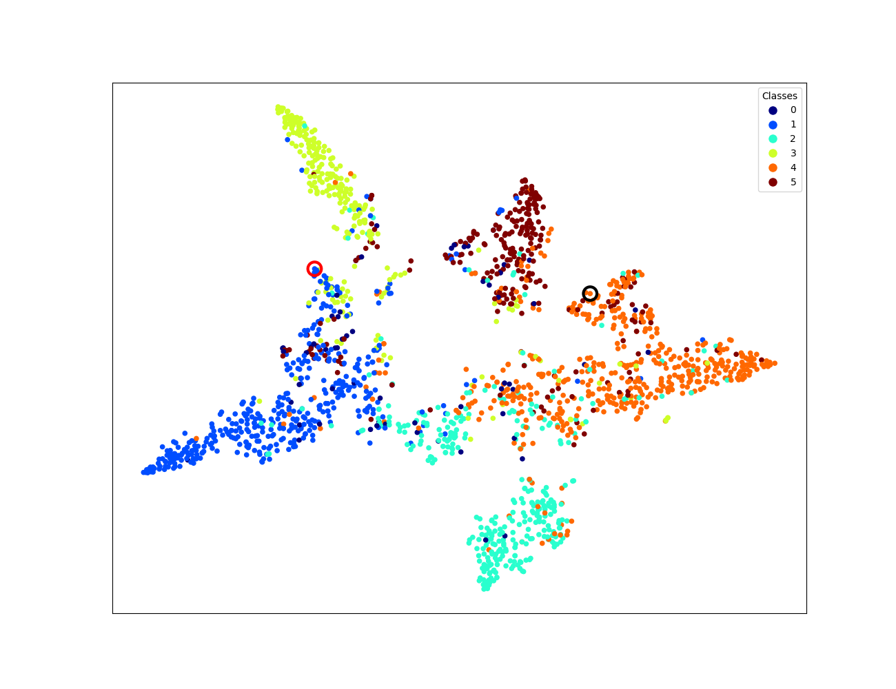
(b) RGCN

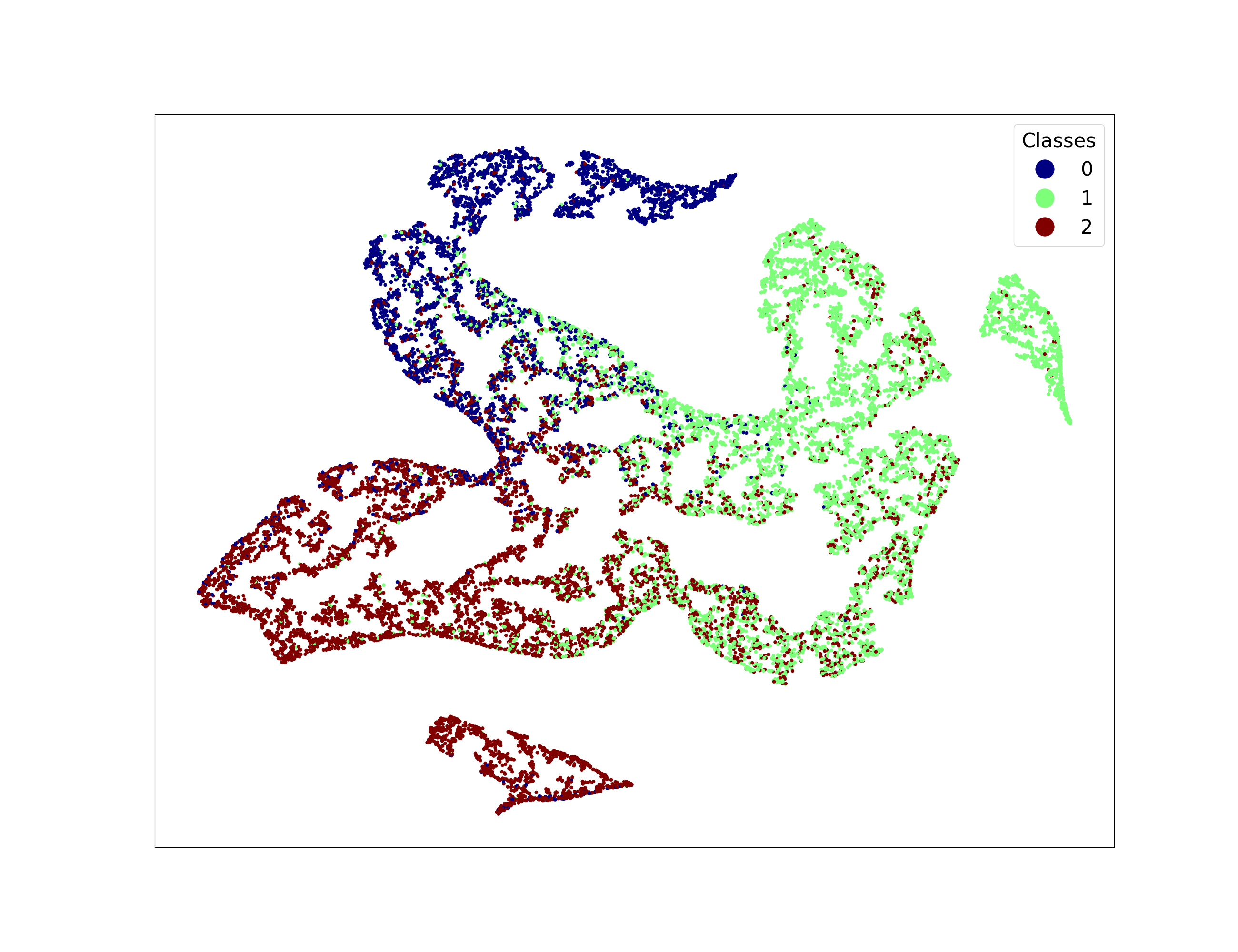
(c)

Figure 4: Visualization results of GCN and RGCN on Cora, Citeseer and Pubmed datasets (from left to right).

To intuitively illustrate the classification performance of our regularized GNN models, we utilize the t-Distributed Stochastic Neighbor Embedding (t-SNE) technique [27] to visualize the predict results of GCN after applying the standard softmax function and RGCN after applying the regularized softmax function. The visualization of classification results for Cora, Citeseer and Pubmed datasets are presented in Figure 4. In these visualizations, each data point represents an individual node from the test sets, with distinct colors denoting the ground truth classes of the nodes. The spatial positions of nodes reflect the projections of high-dimensional embeddings generated by t-SNE. If nodes from different classes are well-separated and nodes from the same class are grouped closely together, it indicates that the model has higher prediction accuracy and better effectiveness.

The outputs generated by RGCN, as shown in Figure 4(b), are more separable than those produced by GCN, as shown in Figure 4(a). For instance, class 2 and class 4 in Cora dataset, and class 4 and class 5 in Citeseer dataset. Several nodes that were misclassified by GCN are indicated with red and black circles; these nodes have been correctly reclassified by RGCN. For example, in Core dataset, a node within a black circle was incorrectly classified by GCN as class 5 but was correctly assigned to class 2 by RGCN. Similarly, in Citeseer dataset, a node within a red circle was misclassified by GCN as class 3 but was accurately reclassified by RGCN as class 1. These results confirm that the regularized softmax function is more effective than the standard softmax function in GNNs for semi-supervised node classification.

4.4.4 Ideal similarity matrix

In this section, to demonstrate the importance of choosing the similarity matrix S in our models, we design an ideal similarity matrix. We assume that the label of each node on the given graph is known and can be used to construct the ideal similarity matrix according to the following rule: if nodes $x_{i}$ and $x_{j}$ belong to the same class, then $\textbf{S}(x_{i},x_{j})=1$; if nodes $x_{i}$ and $x_{j}$ belong to different classes, then $\textbf{S}(x_{i},x_{j})=0$. For better understanding, we provide an example of constructing the ideal similarity matrix from a given graph, as shown in the Figure 5.

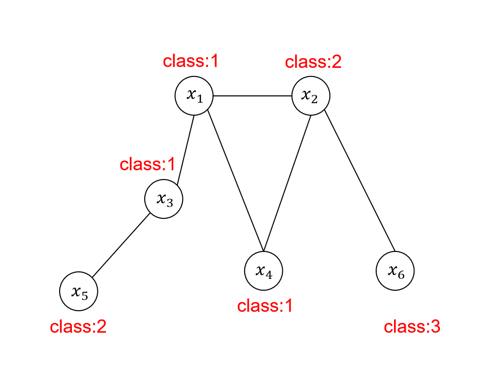
(a) A given graph

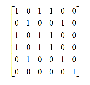
(b) Ideal S

Figure 5: An example of constructing an ideal similarity matrix S.

In Table 7, we present the results of GCN, RGCN and RGCN using the ideal similarity matrix S on a single random dataset split and initialization. We can clearly observe that the classification accuracy achieved with ideal S is notably high, approaching nearly 100%, surpassing both GCN and RGCN. Additionally, the visualizations of RGCN with ideal similarity matrix S on the Cora and Citeseer datasets are displayed in Figure 6. The results show outstanding performance with clear separation between nodes with different labels and high cohesion among nodes sharing the same label. The excellent experimental results further validate the effectiveness of our method, demonstrating that a well-constructed similarity matrix S can significantly enhance the model’s performance.

Table 7: The accuracy (%) over a single random dataset split and initialization.

	Cora	Citeseer
GCN [14]	79.8	73.0
RGCN(ours)	81.8	73.7
RGCN-ideal S	95.1	95.0

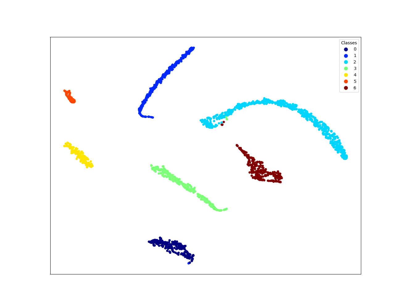
(a) Cora

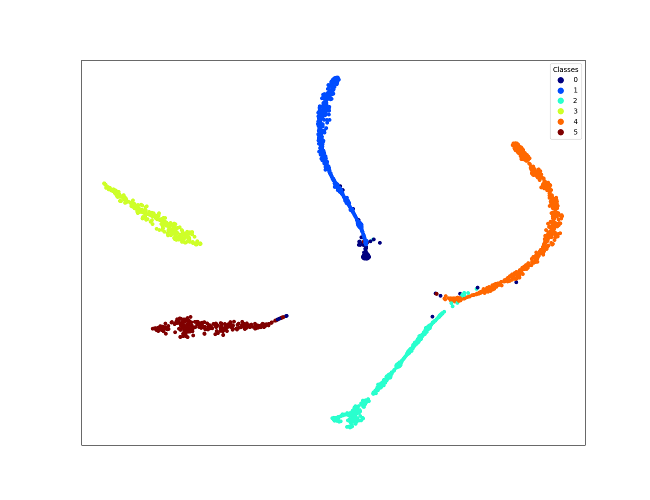
(b) Citeseer

Figure 6: A visualization for the outputs obtained from RGCN with ideal similarity matrix S on the Cora and Citeseer datasets.

5 Conclusion

This paper presents a non-local TV regularized softmax for GNNs aimed at semi-supervised node classification tasks. In our experiments, we apply the proposed regularization method to both GCN and GraphSAGE and observe better performance on assortative and disassortative datasets. To demonstrate the generalization capability of our approach, we conduct experiments over 100 train/validation/test splits and 20 random initializations for each dataset. Additionally, we discuss the significant impact of the similarity matrix on model performance. We propose that designing more effective similarity matrix, rather than relying solely on the adjacency matrix, is a promising direction for future research. For example, developing a learnable similarity matrix could be beneficial for this task. Furthermore, we will explore incorporating STD regularization into the GNN framework.

Calculating the $\mathscr{A}$-subproblem and $\eta$-subproblem in RGNN

For the $\mathscr{A}$-subproblem, we employ the technique of Lagrange multipliers. The Lagrangian function is defined as:

$$\begin{gathered}L=\sum^{K}_{k=1}\{-\langle\mathscr{A}_{k},O_{k}\rangle+\epsilon\langle\mathscr{A}_{k},\log\mathscr{A}_{k}\rangle+\lambda\langle\mathscr{A}_{k},\operatorname{div}_{\textbf{S}}\eta_{k}\rangle\}\\ +\sum^{N}_{i=1}v_{i}\left(\sum^{K}_{k=1}\mathscr{A}_{ik}-1\right),\end{gathered}$$ (27)

where $v_{i}$ are the Lagrange multipliers. Using the first order optimization conditions, we obtain:

$$\frac{\partial L}{\partial\mathscr{A}_{ik}}=-O_{ik}+\epsilon(\log\mathscr{A}_{ik}+1)+\lambda\operatorname{div}_{\textbf{S}}\eta_{ik}+v_{i}=0.$$ (28)

Rearranging, we find:

$$\log\mathscr{A}_{ik}=\frac{O_{ik}-\epsilon-\lambda\operatorname{div}_{\textbf{S}}\eta_{ik}-v_{i}}{\epsilon}.$$ (29)

Thus, we can express $\mathscr{A}_{ik}$ in the following form:

$$\mathscr{A}_{ik}=\exp\left(\frac{O_{ik}-\lambda\operatorname{div}_{\textbf{S}}\eta_{ik}}{\epsilon}\right)\exp\left(\frac{-\epsilon-v_{i}}{\epsilon}\right).$$ (30)

Considering the constraint $\sum^{K}_{k=1}\mathscr{A}_{ik}=1,$ we have:

$$\exp\left({\frac{-\epsilon-v_{i}}{\epsilon}}\right)\sum^{K}_{k=1}\exp\left({\frac{O_{ik}-\lambda\operatorname{div}_{\textbf{S}}\eta_{ik}}{\epsilon}}\right)=1.$$ (31)

Solving for $\exp({\frac{-\epsilon-v_{i}}{\epsilon}})$, we obtain:

$$\exp\left({\frac{-\epsilon-v_{i}}{\epsilon}}\right)=\frac{1}{\sum^{K}_{k=1}\exp\left({\frac{O_{ik}-\lambda\operatorname{div}_{\textbf{S}}\eta_{ik}}{\epsilon}}\right)}.$$ (32)

Substituting (32) into (30), we get:

$$\mathscr{A}_{ik}=\frac{\exp({\frac{O_{ik}-\lambda\operatorname{div}_{\textbf{S}}\eta_{ik}}{\epsilon}})}{\sum^{K}_{\hat{k}=1}\exp({\frac{O_{i\hat{k}}-\lambda\operatorname{div}_{\textbf{S}}\eta_{i\hat{k}}}{\epsilon}})}.$$ (33)

Thus, we can express $\mathscr{A}_{k}$ as:

$$\mathscr{A}_{k}=\text{softmax}\left(\frac{O_{k}-\lambda\operatorname{div}_{\textbf{S}}\eta_{k}}{\epsilon}\right).$$ (34)

For the $\eta$-subproblem, it is equivalent to solving the following minimization problem:

$$\min_{\|\eta_{k}\|_{\infty}\leq 1}\sum^{K}_{k=1}\langle\bigtriangledown_{\textbf{S}}\mathscr{A}_{k},\eta_{k}\rangle.$$ (35)

We solve this using gradient descent and a projection operator:

$$\eta^{t}_{k}=\prod\nolimits_{\|\eta_{k}\|_{\infty}\leq 1}(\eta^{t-1}_{k}-\tau\bigtriangledown\mathscr{A}^{t-1}_{k}).$$ (36)

References

- [1] Jasmijn Bastings, Ivan Titov, Wilker Aziz, Diego Marcheggiani and Khalil Sima’an “Graph convolutional encoders for syntax-aware neural machine translation” In arXiv preprint arXiv:1704.04675, 2017
- [2] Peter Battaglia, Razvan Pascanu, Matthew Lai and Danilo Jimenez Rezende “Interaction networks for learning about objects, relations and physics” In Advances in neural information processing systems 29, 2016
- [3] Hao Chen, Yue Xu, Feiran Huang, Zengde Deng, Wenbing Huang, Senzhang Wang, Peng He and Zhoujun Li “Label-aware graph convolutional networks” In Proceedings of the 29th ACM international conference on information & knowledge management, 2020, pp. 1977–1980
- [4] Mark Craven, Dan DiPasquo, Dayne Freitag, Andrew McCallum, Tom Mitchell, Kamal Nigam and Seán Slattery “Learning to construct knowledge bases from the World Wide Web” In Artificial Intelligence 118.1, 2000, pp. 69–113 DOI: https://doi.org/10.1016/S0004-3702(00)00004-7
- [5] Fadi Dornaika “On the use of high-order feature propagation in Graph Convolution Networks with Manifold Regularization” In Information Sciences 584 Elsevier, 2022, pp. 467–478
- [6] Alex Fout, Jonathon Byrd, Basir Shariat and Asa Ben-Hur “Protein interface prediction using graph convolutional networks” In Advances in neural information processing systems 30, 2017
- [7] Sichao Fu, Weifeng Liu, Kai Zhang, Yicong Zhou and Dapeng Tao “Semi-supervised classification by graph p-Laplacian convolutional networks” In Information Sciences 560 Elsevier, 2021, pp. 92–106
- [8] Sichao Fu, Weifeng Liu, Yicong Zhou and Liqiang Nie “HpLapGCN: Hypergraph p-Laplacian graph convolutional networks” In Neurocomputing 362 Elsevier, 2019, pp. 166–174
- [9] Will Hamilton, Zhitao Ying and Jure Leskovec “Inductive representation learning on large graphs” In Advances in neural information processing systems 30, 2017
- [10] Fan Jia, Jun Liu and Xuecheng Tai “A Regularized Convolutional Neural Network for Semantic Image Segmentation” In ArXiv abs/1907.05287, 2019 URL: https://api.semanticscholar.org/CorpusID:195886329
- [11] Fan Jia, Xue-Cheng Tai and Jun Liu “Nonlocal regularized CNN for image segmentation” In Inverse Problems & Imaging 14.5, 2020, pp. 891–911
- [12] M Tavassoli Kejani, Fadi Dornaika and H Talebi “Graph convolution networks with manifold regularization for semi-supervised learning” In Neural Networks 127 Elsevier, 2020, pp. 160–167
- [13] Diederik P Kingma and Jimmy Ba “Adam: A method for stochastic optimization” In arXiv preprint arXiv:1412.6980, 2014
- [14] Thomas N Kipf and Max Welling “Semi-supervised classification with graph convolutional networks” In arXiv preprint arXiv:1609.02907, 2016
- [15] Jun Liu, Xiangyue Wang and Xue-Cheng Tai “Deep convolutional neural networks with spatial regularization, volume and star-shape priors for image segmentation” In Journal of Mathematical Imaging and Vision 64.6 Springer, 2022, pp. 625–645
- [16] Songtao Liu, Rex Ying, Hanze Dong, Lanqing Li, Tingyang Xu, Yu Rong, Peilin Zhao, Junzhou Huang and Dinghao Wu “Local augmentation for graph neural networks” In International conference on machine learning, 2022, pp. 14054–14072 PMLR
- [17] Galileo Namata, Ben London, Lise Getoor, Bert Huang and U Edu “Query-driven active surveying for collective classification” In 10th international workshop on mining and learning with graphs 8, 2012, pp. 1
- [18] M… Newman “Assortative Mixing in Networks” In Physical Review Letters 89.20 American Physical Society (APS), 2002 DOI: 10.1103/physrevlett.89.208701
- [19] M… Newman “Mixing patterns in networks” In Physical Review E 67.2 American Physical Society (APS), 2003 DOI: 10.1103/physreve.67.026126
- [20] Hongbin Pei, Bingzhe Wei, Kevin Chen-Chuan Chang, Yu Lei and Bo Yang “Geom-gcn: Geometric graph convolutional networks” In arXiv preprint arXiv:2002.05287, 2020
- [21] Wenjie Pei, Weina Xu, Zongze Wu, Weichao Li, Jinfan Wang, Guangming Lu and Xiangrong Wang “Saliency-aware regularized graph neural network” In Artificial Intelligence 328 Elsevier, 2024, pp. 104078
- [22] Herbert E. Robbins “A Stochastic Approximation Method” In Annals of Mathematical Statistics 22, 1951, pp. 400–407 URL: https://api.semanticscholar.org/CorpusID:16945044
- [23] Leonid I. Rudin, Stanley Osher and Emad Fatemi “Nonlinear total variation based noise removal algorithms” In Physica D: Nonlinear Phenomena 60.1, 1992, pp. 259–268 DOI: https://doi.org/10.1016/0167-2789(92)90242-F
- [24] Prithviraj Sen, Galileo Namata, Mustafa Bilgic, Lise Getoor, Brian Galligher and Tina Eliassi-Rad “Collective classification in network data” In AI magazine 29.3, 2008, pp. 93–93
- [25] Oleksandr Shchur, Maximilian Mumme, Aleksandar Bojchevski and Stephan Günnemann “Pitfalls of graph neural network evaluation” In arXiv preprint arXiv:1811.05868, 2018
- [26] Xiuzhi Tian, Chris HQ Ding, Sibao Chen, Bin Luo and Xin Wang “Regularization graph convolutional networks with data augmentation” In Neurocomputing 436 Elsevier, 2021, pp. 92–102
- [27] Laurens Van der Maaten and Geoffrey Hinton “Visualizing data using t-SNE.” In Journal of machine learning research 9.11, 2008
- [28] Petar Veličković, Guillem Cucurull, Arantxa Casanova, Adriana Romero, Pietro Lio and Yoshua Bengio “Graph attention networks” In arXiv preprint arXiv:1710.10903, 2017
- [29] Bin Wang, LvHang Cheng, JinFang Sheng, ZhengAng Hou and YaoXing Chang “Graph convolutional networks fusing motif-structure information” In Scientific Reports 12.1 Nature Publishing Group UK London, 2022, pp. 10735
- [30] Keyulu Xu, Weihua Hu, Jure Leskovec and Stefanie Jegelka “How powerful are graph neural networks?” In arXiv preprint arXiv:1810.00826, 2018
- [31] Rex Ying, Ruining He, Kaifeng Chen, Pong Eksombatchai, William L Hamilton and Jure Leskovec “Graph convolutional neural networks for web-scale recommender systems” In Proceedings of the 24th ACM SIGKDD international conference on knowledge discovery & data mining, 2018, pp. 974–983
- [32] Li Zhang and Haiping Lu “A feature-importance-aware and robust aggregator for GCN” In Proceedings of the 29th ACM International Conference on Information & Knowledge Management, 2020, pp. 1813–1822