Optimal control of a kinetic model describing social interactions on a graph

Abstract

In this paper we introduce the optimal control of a kinetic model describing agents who migrate on a graph and interact within its nodes exchanging a physical quantity. As a prototype model, we consider the spread of an infectious disease on a graph, so that the exchanged quantity is the viral-load. The control, exerted on both the mobility and on the interactions separately, aims at minimising the average macroscopic viral-load. We prove that minimising the average viral-load weighted by the mass in each node is the most effective and convenient strategy. We consider two different interactions: in the first one the infection (gain) and the healing (loss) processes happen within the same interaction, while in the second case the infection and healing result from two different processes. With the appropriate controls, we prove that in the first case it is possible to stop the increase of the disease, but paying a very high cost in terms of control, while in the second case it is possible to eradicate the disease. We test numerically the role of each intervention and the interplay between the mobility and the interaction control strategies in each model.

1 Introduction

Interactions happening within—or among—social groups often present traits of heterogeneity: whenever either the groups or the interactions themselves are not homogeneous, labeling the social groups’ elements is a useful abstraction, along with building a relational model of members’ interactions based on those labels. In this context, network theory is a natural framework [36], allowing to study different phenomena from disease spreading [28, 40] to dissemination of information [35, 9] to movement (local, i.e., traffic [38, 4] and global, i.e., migration [43, 22]). In particular, developing models to analyze and control dynamics taking place on large networks has become one of the most relevant aspects in contemporary research in applied mathematics, especially related to epidemiology.

Kinetic theory [11], emerging from the field of statistical mechanics of particle physics, has established itself in the last decades as one of the most powerful ways to model the behavior of systems of a large number of interacting agents and to derive sound macroscopic models inheriting the characteristics of the implemented universal microscopic dynamics [39]. Its characteristics makes it suitable to employ in order to study dynamics on underlying networks, either for diseases spreading [5], opinion formation [1, 2, 18] or more general type of interactions [37, 10].

In the field of epidemiology, viral-load-based frameworks are employed classically, especially in studies on chronic infections like HIV [25, 27], but they are studied also for acute settings in view of the usefulness of quantitative data over qualitative clinical descriptions for policy making or therapy design [23, 41]. For this reason, and also for its natural description within kinetic theory, substantial mathematical research on viral-load-based models has been conducted recently, see, e.g., [32, 33] for a more general introduction, [14, 15] for compartmental-based models and [8] for a data-driven approach.

For what concerns optimal control theory of diseases on networks, instead, we refer the reader to the recent works on homogeneous populations [20, 26, 30], on heterogeneous populations [42], to works on information dissemination like, e.g., [19, 31, 24] and to opinions in a kinetic setting like, e.g., [1]. Moreover, for a short list of recent papers on optimal control within the framework of kinetic theory on related topics see, e.g., [3, 21, 16] and references therein.

In view of the importance of this topic for the aforementioned reasons, in this paper we follow up the model presented in [33], where the authors propose a Boltzmann-type kinetic model for the spreading of diseases on a network, based on the exchange of viral load. Our contribution to the model in [33] is to devise optimal control strategies to mitigate the infection on the network. To this aim, we rely on the method used in [3].

The manuscript outline is as follows. As in the original work [33], in Section 2, we consider a strongly connected graph: each agent belongs to exactly one of its vertices (or nodes) and can move from node to node with a certain probability, prescribed by a transition matrix. Agents can only interact—pairwise—with their peers belonging to their same node; each binary interaction consists in an exchange of viral load, representing the contagion dynamics. In Section 3, we start by considering a control policy intervening on agents’ mobility, i.e., we construct a suitably controlled transition matrix. Then we proceed to devise in-node control strategies to affect agents’ interactions within the same vertex. Our results show that the prototypical model of [33], while useful to gain insight by binary exchange contagion dynamics, might be too simplistic to depict a fully realistic infection phenomenon in which individuals can actually recover, and to give rise to satisfactory controlling results in a challenging spreading scenario. For this reason, in Section 4 we modify the interaction dynamics to incorporate a healing process, again expressed as a suitable kind of binary interaction. In this new setting, we devise a different in-node control strategy, of which we can prove it achieves the complete eradication of the disease from the network, under appropriate assumptions.

We present in Section 5 several numerical experiments to support our theoretical findings and we also showcase an application of the new infection-healing dynamics on real-world data. Finally, we conclude the manuscript by commenting on the presented results and we outline some possible future research directions.

2 Mathematical modeling of interactions on a graph

In this section, we revise the basic kinetic-like model (without control) for social interactions on a graph. We summarise the results presented in [33] concerning the emerging behavior of the system that can be studied by analysing the macroscopic equations that can be derived from the underlying kinetic description.

2.1 Kinetic description

Let us consider a large system of interacting individuals migrating on a network, which is modelled by a graph with a finite number of vertices and edges. In particular, we introduce a weighted graph $G=(\mathcal{I},E,A)$, where $\mathcal{I}$ is the set of the nodes that is a finite ordered index set with $\left\lvert\mathcal{I}\right\rvert=n\in\mathbb{N}$, for instance $\mathcal{I}=\{1,\,\dots,\,n\}\subset\mathbb{N}$. The set $E$ is the set of the edges, while $A=A_{ij}$ is the set of the weights that can be assigned to each edge. Then $A$ allows to define the transition matrix $P$ that is defined as

$$P_{ij}\coloneqq\operatorname{Prob}(j\to i):=\dfrac{A_{ij}}{\sum_{i\in\mathcal{I}}A_{ij}}\in[0,1],\qquad i,j\in\mathcal{I},$$ (1)

and thus satisfies

$$\sum_{i\in\mathcal{I}}P_{ij}=1,\qquad\forall i\in\mathcal{I}.$$ (2)

The transition matrix $\mathbf{P}\coloneqq[P_{ij}]_{i,j\in\mathcal{I}}\in\mathbb{R}^{n\times n}$ is, by definition (2), left stochastic. Moreover, we shall consider strongly connected graphs, which means that for any two nodes, there exists at least one directed path that connects them. Notice that a graph is strongly connected if and only if $\mathbf{P}$ is irreducible [34].

The agents are assumed to be characterised by a physical quantity $v\in\mathbb{R}_{+}$ and to be located on the nodes of the graph $G$. As a consequence, the agents are characterized by a microscopic state $(x,v)\in\mathcal{I}\times\mathbb{R}_{+}$. The label $x\in\mathcal{I}$, denoting the vertex on which the agent is located, may change as a consequence of possible migrations among the nodes of the graph. Hence, the displacements of the agents from one vertex to another are described as a Markov-type jump process through the transition probability $P_{ij}$ representing the probability to jump from vertex $j$ to vertex $i$. Conversely, the physical quantity $v\in\mathbb{R}_{+}$ can be exchanged as a consequence of binary interactions. In the present case $v$ represents the viral load. In particular, it is assumed that individuals may interact only when on the same node $x=i$. In order to have easily manageable interaction rules and having the aim of studying the emerging properties of the system, we consider linear interaction rules defined as

$$v^{\prime}=(1-\nu_{1}^{i}+\eta)v+\nu_{2}^{i}v_{*},\qquad v_{*}^{\prime}=(1-\nu_{1}^{i}+\eta_{\ast})v_{*}+\nu_{2}^{i}v,$$ (3)

where $v$, $v_{*}$ represent the pre-interaction states of two interacting individuals and $v^{\prime}$, $v_{*}^{\prime}$ their post-interaction states. In (3), $\nu_{1}^{i},\nu_{2}^{i}\in[0,1]$ are the exchange parameters describing the deterministic part of the interaction that may depend on the node $i$, while $\eta,\eta_{\ast}$ are white noises taking into account the possible stochastic fluctuations. Moreover, the two microscopic processes leading to the migration across the nodes of the graph and to the binary exchange process are assumed to be stochastically independent and happening with frequencies $\chi$ and $\mu$ respectively.

The evolution equation of each $f_{i}=f_{i}(v,t):\mathbb{R}_{+}\times\mathbb{R}_{+}\to\mathbb{R}_{+}$, which is the distribution of $v$ in each node $i$, is shown to be

$$\frac{d}{dt}\int_{{\mathbb{R}_{+}}}\varphi(v)f_{i}(v,t)\,dv =\chi\int_{{\mathbb{R}_{+}}}\varphi(v)\biggl{(}\sum_{j\in\mathcal{I}}P_{ij}f_{j}(v,t)-f_{i}(v,t)\biggr{)}\,dv$$ (4)

$$+\mu\int_{{\mathbb{R}_{+}}}\varphi(v)Q(f_{i},f_{i})(v,t)\,dv,\qquad i\in\mathcal{I},$$

where $\varphi\colon{\mathbb{R}_{+}}\to\mathbb{R}$ is a test function and $Q(f_{i})$ is the so-called collisional operator, defined in weak form by

$$\int_{{\mathbb{R}_{+}}}\varphi(v)Q(f_{i},f_{i})(v,t)\,dv=\int_{{\mathbb{R}_{+}}}\!\int_{{\mathbb{R}_{+}}}\langle\varphi(v^{\prime})-\varphi(v)\rangle f_{i}(v,t)f_{i}(v_{*},t)\,dv_{*}\,dv.$$ (5)

2.2 Aggregate description

In the rest of the manuscript, we will be interested in some aggregate average quantities, namely

$$\rho_{i}(t)\coloneqq\int_{{\mathbb{R}_{+}}}f_{i}(v,t)\,dv\geq 0,\qquad\rho_{i}(t)m_{i}(t)\coloneqq\int_{{\mathbb{R}_{+}}}vf_{i}(v,t)\,dv,$$ (6)

which are the density and first moment of the individuals on the $i$-th node of the graph, respectively.

Setting $\varphi=1$ in (4) allows to obtain

$$\frac{d\rho_{i}}{dt}=\chi\left(\sum_{j\in\mathcal{I}}P_{ij}\rho_{j}-\rho_{i}\right),\qquad i\in\mathcal{I},$$ (7)

which in vector notation reads

$$\frac{d\bm{\rho}}{dt}=\chi(\mathbf{P}-\mathbf{I})\bm{\rho},$$ (8)

with $\bm{\rho}:=(\rho_{i})_{i\in\mathcal{I}}$. First of all we remark that

$$\frac{d}{dt}\|\bm{\rho}(t)\|_{1}:=\frac{d}{dt}\sum_{i\in\mathcal{I}}\rho_{i}(t)=0,$$

i.e. the $\ell^{1}$-norm of $\bm{\rho}$, i.e. the quantity $\|\bm{\rho}\|_{1}:=\sum_{i\in\mathcal{I}}\rho_{i}$, is conserved in time, which, physically, means conservation of mass across the graph. From (8) we can investigate the stationary mass distribution $\bm{\rho}^{\infty}\in\mathbb{R}^{n}_{+}$ emerging for large times, namely the vector satisfying the equation

$$(\mathbf{P}-\mathbf{I})\bm{\rho}^{\infty}=\mathbf{0}.$$ (9)

In [33], the authors studying the eigenvalues-eigenvector properties of the transition matrix $\mathbf{P}$ and by applying the Perron-Frobenius theory, prove that

Proposition 1.

Let $\mathbf{P}$ be irreducible. There exists a unique physically admissible solution $\bm{\rho}^{\infty}\in\mathbb{R}^{n}_{+}$ to (9), which is a stable and attractive asymptotic density distribution for (8).

Remark 2.

The uniqueness is fixed by conservation of mass across the graph. Specifically, we have that, given $\bm{\rho^{0}}=[\rho_{1}^{0},...,\rho^{0}_{n}]$ the initial condition, then we have that

$$\|\bm{\rho}\|_{1}=\|\bm{\rho}^{0}\|_{1}.$$

Conversely, setting $\varphi(v)=v$ in (4) we may investigate the evolution of the first moment $\rho_{i}m_{i}$ which turns out to satisfy the equation

$$\frac{d}{dt}(\rho_{i}m_{i})=\chi\left(\sum_{j\in\mathcal{I}}P_{ij}\rho_{j}m_{j}-\rho_{i}m_{i}\right)+\mu(\nu_{2}^{i}-\nu_{1}^{i})\rho_{i}^{2}m_{i}.$$ (10)

Moreover, the evolution of the average

$$m_{i}(t):=\frac{1}{\rho_{i}(t)}\int_{\mathbb{R}_{+}}vf_{i}(v,t)\,dv,$$

is

$$\frac{d}{dt}m_{i}=\frac{\chi}{\rho_{i}}\sum_{j\in\mathcal{I}}P_{ij}\rho_{j}(m_{j}-m_{i})+\mu(\nu^{i}_{2}-\nu^{i}_{1})\rho_{i}m_{i}.$$ (11)

As expected, the average varies because of the sum of the two independent contributions, related to the migration on the graph and to the evolution of the average physical quantity, respectively, as

$$\frac{d}{dt}m_{i}=\left[\frac{d}{dt}m_{i}\right]_{\chi}+\left[\frac{d}{dt}m_{i}\right]_{\mu},$$ (12)

where

$$\left[\frac{d}{dt}m_{i}\right]_{\chi}=\frac{\chi}{\rho_{i}}\sum_{j\in\mathcal{I}}P_{ij}\rho_{j}(m_{j}-m_{i}),$$ (13)

and

$$\left[\frac{d}{dt}m_{i}\right]_{\mu}=\mu(\nu^{i}_{2}-\nu^{i}_{1})\rho_{i}m_{i}.$$ (14)

Moreover, as a consequence of (2), we have that the variation of the total average on the graph is only due to the interactions inside the nodes, as

$$\frac{d}{dt}\sum_{i\in\mathcal{I}}\rho_{i}m_{i}=\mu\sum_{i\in\mathcal{I}}\rho_{i}^{2}m_{i}(\nu_{2}^{i}-\nu_{1}^{i}).$$ (15)

As a consequence of the latter, it is possible to prove that

Proposition 3.

Assume the graph is strongly connected and that $\nu_{1}^{i}=\nu_{1},\nu_{2}^{i}=\nu_{2}$. When $t\rightarrow\infty$, the solution $m_{i}$ of (11) obeys one of the following cases:

1. If $\nu_{1}>\nu_{2}$ then $m_{i}\rightarrow 0$ for all $i\in\mathcal{I}$ and $\bm{m}^{\infty}=\bm{0}$ is a stable and attractive solution for (11).

2. If $\nu_{1}<\nu_{2}$ then the solution $m_{i}$ of (11) satisfies $m_{i}\rightarrow\infty$ for some $i\in\mathcal{I}$.

3. If $\nu_{1}=\nu_{2}$ then $\displaystyle\sum_{i\in\mathcal{I}}\rho_{i}m_{i}$, being the evolution of $\rho_{i}m_{i}$ described by (10), is constant in time. Moreover, there exists a unique stable and attractive equilibrium configuration for $\bm{m}^{\infty}$ and in particular $m_{i}^{\infty}=\displaystyle\sum_{j\in\mathcal{I}}\rho_{j}m_{j}$ for all $i\in\mathcal{I}$.

Proof.

The first two points have been proved in [33]. We then prove the third point, as it is slightly more general than in [33]. Let $\nu_{1}=\nu_{2}$. If either $\bm{\rho}(0)=\mathbf{0}$ or $\bm{m}(0)=\mathbf{0}$, equation (15) gives the claim immediately. Otherwise, we can conveniently rewrite equation (10) as

$$\frac{d\beta_{i}}{dt}=\chi\left(\sum_{j\in\mathcal{I}}P_{ij}\beta_{j}-\beta_{i}\right),\qquad i\in\mathcal{I},$$ (16)

where we introduced the quantities $\beta_{i}$, defined as

$$\beta_{i}(t)\coloneqq\frac{\rho_{i}m_{i}(t)}{\displaystyle\sum_{j\in\mathcal{I}}\rho_{j}m_{j}(t)}.$$ (17)

Since $\nu_{1}=\nu_{2}$, equation (15) implies the conservation of the total first moment $\rho_{i}m_{i}$, so that the denominator in equation (17) is a positive constant and (16) is well defined. In particular, we also have that $\beta_{i}\in[0,1]$ for all $i\in\mathcal{I}$ and $\sum_{i\in\mathcal{I}}\beta_{i}=1$. Therefore, due to the irreducibility of the matrix $\mathbf{P}$, we can apply Perron-Frobenius theorem on the vector form of equation (16)

$$\frac{d\bm{\beta}}{dt}=\chi(\mathbf{P}-\mathbf{I})\bm{\beta}$$

to obtain the existence of a unique, stable and attractive positive equilibrium point $\beta_{i}^{\infty}\in\mathbb{R}_{+}^{n}$. Moreover, Perron-Frobenius theorem actually tells us that $\bm{\beta}^{\infty}=\bm{\rho}^{\infty}$, since they must be scalar multiples and they share the same norm. This implies that

$$\rho_{i}^{\infty}m_{i}^{\infty}=\rho_{i}^{\infty}\sum_{j\in\mathcal{I}}\rho_{j}m_{j},$$

and we conclude setting the equilibrium point for the node average as

$$m_{i}^{\infty}=\begin{cases}0&\text{if }\rho_{i}^{\infty}=0,\\ \displaystyle\sum_{j\in\mathcal{I}}\rho_{j}m_{j}&\text{otherwise}.\end{cases}$$ (18)

∎

Remark 4.

Proposition 3 allows to detect the asymptotic value of the average viral load in the case $\nu_{2}=\nu_{1}$ that is the same in each node as proved by (18), and shown numerically in Figure 1.

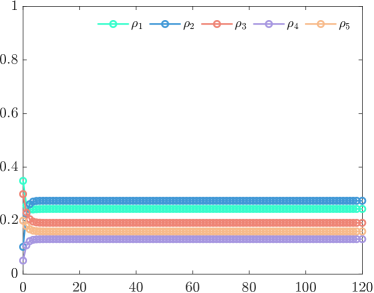
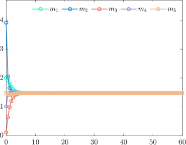
Figure 1: Left to right: example of evolution in time of number of agents and average viral load in the case $\nu_{1}^{i}=\nu_{2}^{i}=1/2$ for all $i\in\mathcal{I}$. The numerical test shows accordance with Proposition 3. Refer to Section 5.1 for more details about the simulation.

In the case of node dependent exchange parameters, the authors in [33] prove that

Proposition 5.

Let the graph be strongly connected and let us assume that $\mu=\dfrac{1}{\varepsilon}$, $\chi=1$, where $\varepsilon\ll 1$ in (4). Then,

• Assume $\nu_{1}^{i}>\nu_{2}^{i}$ for all $i\in\mathcal{I}-\{i_{\ast}\}$ and $\nu_{1}^{i_{*}}=\nu_{2}^{i_{*}}$. Then $m_{i}\rightarrow 0$ for all $i\in\mathcal{I}$, in particular also for $i=i_{\ast}$;

• Assume $\nu_{1}^{i}=\nu_{2}^{i}$ for all $i\in\mathcal{I}-\{i_{\ast}\}$ and $\nu_{1}^{i_{*}}>\nu_{2}^{i_{*}}$. Let moreover $\mathcal{I}_{\ast}=\{j\in\mathcal{I}:P_{i_{\ast},j}>0\}$. Then $m_{i}\rightarrow 0$ for all $i\in\mathcal{I}_{*}$;

• Assume $\nu_{1}^{i_{*}}<\nu_{2}^{i_{*}}$ for some $i_{\ast}\in\mathcal{I}$. Then $m_{i}\rightarrow\infty$ when $t\rightarrow\infty$ for all $i\in\mathcal{I}$ s.t. $\nu_{1}^{i}\leq\nu_{2}^{i}$ while $m_{i}\rightarrow 0$ when $t\rightarrow\infty$ for all $i\in\mathcal{I}$ s.t. $\nu_{1}^{i}>\nu_{2}^{i}$.

The Proof of the latter (see [33]) relies on the use of classical arguments of kinetic theory, such as the hydrodynamic regime and collision invariants. Specifically, the regime $\mu=\dfrac{1}{\varepsilon}$, $\chi=1$ corresponds to the one in which local interactions within the vertices of the graph are much more frequent than jumps from node to node, that are assimilated to the free particle transport in classical kinetic theory, and that happens on a slower time scale.

3 The control problem

In this section, we implement a control on the kinetic-like equations presented in the previous section. The control has the aim of mitigating the diffusion of the infectious disease in each node and across the graph. As the state of the individual with respect to the disease is characterised by the viral-load $v\in\mathbb{R}_{+}$, we shall implement such a control by controlling some quantity related to the average viral-load. As we want to control the evolution of the average in each node, we bear in mind that such an evolution in each node depends on both (independent) processes, i.e. the binary interactions leading to exchange of the physical quantity $v$ and the migration across the nodes. As a consequence, we consider two kinds of control: $u_{i}^{\chi}$, a multiplicative control term on $P_{ij}$—with the idea from a modeling point of view of controlling the mobility from node to node—and a multiplicative control $u_{i}^{\mu}$ on the binary interactions to mimic containment measures within nodes.

3.1 Control on the transition matrix

Let us define the controlled transition matrix

$$P_{ij}^{u}=\begin{cases}P_{ij}\cdot(1-u_{i}^{\chi})&i\neq j,\\[5.69046pt] 1-\displaystyle\sum_{\begin{subarray}{c}k\in\mathcal{I}\\ k\neq i\end{subarray}}P_{ki}^{u}&\text{otherwise},\end{cases}$$ (19)

where $u_{i}^{\chi}$ is the control on the migration dynamics implemented in order to mitigate the incoming migration in each node $i\in\mathcal{I}$. We shall consider $u_{i}^{\chi}\in[0,1]$, so that $(1-u_{i}^{\chi})\in[0,1]$ with the idea of expressing the interaction/migration limitations as a percentage of the normal regime. The optimality conditions defining $u_{i}^{\chi}$ will be discussed later, and will be based on the infection condition in node $i$, as it is reasonable to hamper individuals from migrating to node $i$ if the infection there is too high. The modeling choice $u_{i}^{\chi}\in[0,1]$ allows to prove that the entries of the controlled matrix are non-negative and smaller than one, so that they can be probabilities. In fact, the following Proposition holds.

Lemma 6.

If $u_{i}^{\chi}\in[0,1]$ for all $i\in\mathcal{I}$, then $P_{ij}^{u}\in[0,1]$ for all $i,j\in\mathcal{I}$.

Proof.

As $P_{ij}\in[0,1]$ and $u_{i}^{\chi}\in[0,1]$ it is clear that $P_{ij}^{u}\in[0,1]$ for all $j\neq i$. Then, we need to check that $P_{ii}^{u}\in[0,1]$ for all $i\in\mathcal{I}$. Clearly, $1-\sum_{k\neq i}P_{ki}^{u}\leq 1$, while we have that

$$1-\displaystyle\sum_{\begin{subarray}{c}k\in\mathcal{I}\\ k\neq i\end{subarray}}P_{ki}^{u}=1-\displaystyle\sum_{\begin{subarray}{c}k\in\mathcal{I}\\ k\neq i\end{subarray}}P_{ki}(1-u_{k}^{\chi})=P_{ii}+\displaystyle\sum_{\begin{subarray}{c}k\in\mathcal{I}\\ k\neq i\end{subarray}}P_{ki}\,u_{k}^{\chi}\geq 0,$$

where in the last equality we have used $1-\displaystyle\sum_{\begin{subarray}{c}k\in\mathcal{I}\\ k\neq i\end{subarray}}P_{ki}=P_{ii}$ that follows from (2). ∎

As $P_{ij}^{u}\in[0,1]$ for all $i,j\in\mathcal{I}$, we can now remark that $\mathbf{P}^{\mathbf{u}}$ is a left stochastic matrix by construction, thanks to the definition of $P_{ii}^{u}$ in (19), i.e. its satisfies

$$\sum_{\begin{subarray}{c}i\in\mathcal{I}\end{subarray}}P^{u}_{ij}=1,\qquad\forall j\in\mathcal{I}.$$ (20)

The diagonal entry $P_{ii}^{u}$ can be explicitly determined from (19) using (20)

$$P_{ii}^{u}=P_{ii}+\sum_{\begin{subarray}{c}k\in\mathcal{I}\\ k\neq i\end{subarray}}u_{k}P_{ki}.$$ (21)

We remark that, while $(1-u_{k}^{\chi})$ diminishes the mobility from node $i$ to $k$, as soon as at least one $k\neq i$ satisfies $u_{k}^{\chi}>0$, then $P_{ii}^{u}>P_{ii}$, i.e. the probability of staying in the same node is higher.

Furthermore, the probability of reaching node $i$ in the controlled and uncontrolled scenarios are related as follows

$$\sum_{\begin{subarray}{c}k\in\mathcal{I}\\ k\neq i\end{subarray}}P^{u}_{ik}=(1-u_{i}^{\chi})\displaystyle\sum_{\begin{subarray}{c}k\in\mathcal{I}\\ k\neq i\end{subarray}}P_{ik},$$

thus determining $(1-u_{i}^{\chi})$ to be the total mobility reduction rate to node $i$. Moreover, we have that the control may preserve the irreducibility of the transition matrix under a suitable condition.

Proposition 7.

If we set $u_{i}^{\chi}\in[0,1)$ for all $i\in\mathcal{I}$ and consider an irreducible transition matrix $P_{ij}$, then $P_{ij}^{u}$ is irreducible.

Proof.

It is straightforward to see that if $\mathbf{P}$ is associated to a strongly connected graph, then the graph associated to $\mathbf{P}^{u}$ is still strongly connected and, thus $\mathbf{P}^{u}$ is irreducible. ∎

Remark 8.

Of course, the extremal choice $u_{i}^{\chi}=1$ (that corresponds to a hundred percent restrictions) would have the effect of disconnecting the network, thus ceding the irreducibility.

3.2 Control in each node

We consider two independent controls on the migration dynamics and on the binary interactions, as they are independent processes, and controlling both with the same control could be over expensive. We then define the controlled problem as

$$\frac{d}{dt}\int_{\mathbb{R}_{+}}\varphi(v)f_{i}(v,t)\,dv =\mu_{i}\,\left\langle\int_{\mathbb{R}_{+}}\!\int_{\mathbb{R}_{+}}(\varphi(v^{\prime})-\varphi(v))f_{i}(t,v)f_{i}(t,v_{*})\,dv_{*}\,dv\right\rangle$$ (22)

$$\hphantom{{}=}+\chi\int_{\mathbb{R}_{+}}\varphi(v)\bigl{[}P_{ij}^{u}f_{j}(t,v)-f_{i}(t,v)\bigr{]}\,dv,$$

where the control matrix $P_{ij}^{u}$ is defined by equation (19), while the control $\mu_{i}$ on the binary interactions is defined by

$$\mu_{i}:=\mu(1-u_{i}^{\mu}).$$ (23)

The latter has the effect of reducing the interaction rate inside each node. The optimality conditions defining $u_{i}^{\mu}$ will be discussed later.

Next, we analyse the controlled macroscopic equations. We shall denote by the apex ^u the macroscopic quantities related to the controlled problem (22). Setting $\varphi=1$ in (22), we obtain

$$\frac{d}{dt}\rho_{i}^{u} =\chi\biggl{[}\sum_{j\in\mathcal{I}}P_{ij}^{u}\rho_{j}^{u}-\rho_{i}^{u}\biggr{]}=\chi\biggl{[}\sum_{\begin{subarray}{c}j\in\mathcal{I}\\ j\neq i\end{subarray}}(P_{ij}^{u}\rho_{j}^{u}-P_{ji}^{u}\rho_{i}^{u})\biggr{]},$$

$$=\chi\biggl{[}(1-u_{i}^{\chi})\sum_{\begin{subarray}{c}j\in\mathcal{I}\\ j\neq i\end{subarray}}P_{ij}\rho_{j}-\sum_{\begin{subarray}{c}j\in\mathcal{I}\\ j\neq i\end{subarray}}P_{ji}(1-u_{j}^{\chi})\rho_{i}\biggr{]},$$

that highlights the fact that $(1-u_{i}^{\chi})$ in the gain term regulates the incoming migration, while the terms $(1-u_{j}^{\chi}),\,j\neq i$ in the loss term diminishes the outgoing flux.

Setting $\varphi=v$ in (22) we obtain

$$\frac{d}{dt}\rho_{i}^{u}(t)m_{i}^{u}(t)=\chi\biggl{[}\sum_{j\in\mathcal{I}}P_{ij}^{u}\rho_{j}^{u}(t)m_{j}^{u}(t)-\rho_{i}^{u}(t)m_{i}^{u}(t)\biggr{]}+\mu(1-u_{i}^{\mu})(\nu^{i}_{2}-\nu^{i}_{1})\rho_{i}^{u^{2}}(t)m_{i}^{u}(t),$$ (24)

and, also

$$\frac{d}{dt}m_{i}^{u}(t)=\chi\biggl{[}\sum_{\begin{subarray}{c}j\in\mathcal{I}\\ j\neq i\end{subarray}}P_{ij}^{u}\frac{\rho_{j}^{u}(t)}{\rho_{i}^{u}(t)}\bigl{(}m_{j}^{u}(t)-m_{i}^{u}(t)\bigr{)}\biggr{]}+\mu(1-u_{i}^{\mu})(\nu^{i}_{2}-\nu^{i}_{1})\rho_{i}^{u}(t)m_{i}^{u}(t),$$ (25)

i.e.

$$\frac{d}{dt}m_{i}^{u}=(1-u_{i}^{\chi})\left[\frac{d}{dt}m_{i}\right]_{\chi}+(1-u_{i}^{\mu})\left[\frac{d}{dt}m_{i}\right]_{\mu},$$

where in the right hand side the quantities are defined in (13)-(14).

Remark 9.

We remark that, for both the evolution of the masses and of the averages, the controls $1-u_{i}^{\chi},1-u_{i}^{\mu}\in[0,1]$ reduce the time variation rate, without inverting the natural trend. Only if we allow $u_{i}^{\mu},u_{i}^{\chi}=1$, the control has the effect of stopping the time evolution of both masses and averages. This is why we also consider a control on the migration mechanism.

Remark 10.

We remark that, like in the uncontrolled case, as $\mathbf{P}^{\mathbf{u}}$ is a left stochastic matrix, then the total average on the graph only depends on the binary exchange process, i.e.

$$\frac{d}{dt}\sum_{i\in\mathcal{I}}\rho_{i}^{u}m_{i}^{u}=\mu\sum_{i\in\mathcal{I}}(1-u_{i}^{\mu})\rho_{i}^{u^{2}}m_{i}^{u}(\nu_{2}^{i}-\nu_{1}^{i}).$$ (26)

thus suggesting that a mere control on the interaction rate $\mu$ is sufficient in order to mitigate the evolution of the total average. Moreover, we have that, as the microscopic processes are independent and the evolution of the physical quantity is mainly due to the binary exchange process, only controlling the migration mechanism is not enough. However, as the travelling individuals carry on with them their state $v$ while migrating across the nodes, in case of a mere control on the the interaction rate, the control would need to be stronger in order to mitigate the propagation of large values of $v$.

3.3 Optimality conditions

From now on, we drop the apex ^u on the average quantities $\rho_{i},\rho_{i}m_{i}$ of the controlled problem (22). We now want to find the optimal control $\bar{u}_{i}^{\mu},\bar{u}_{i}^{\chi}$, similarly to [3]. Let us then consider the problem with a discretisation in time

$$\int_{\mathbb{R}_{+}}\varphi(v)f_{i}(t+h,v)\,dv =\int_{\mathbb{R}_{+}}\varphi(v)f_{i}(t,v)\,dv+h\chi\int_{\mathbb{R}_{+}}\varphi(v)\bigl{[}\sum_{j\in\mathcal{I}}P_{ij}^{u}f_{i}(t,v)-f_{i}(t,v)\bigr{]}\,dv$$ (27)

$${\hphantom{{}={}}}+h\mu(1-u_{i}^{\mu})\,\left\langle\int_{\mathbb{R}_{+}}\!\int_{\mathbb{R}_{+}}(\varphi(v^{\prime})-\varphi(v))f_{i}(t,v)f_{i}(t,v_{*})\,dv_{\ast}\,dv\right\rangle.$$

We consider the cost functional:

$$\mathcal{J}_{h}^{i}(u_{i}^{\chi},u_{i}^{\mu},\rho_{i}m_{i})=\psi(\rho_{i}m_{i}(t+h))+\frac{1}{2}\nu^{\chi}{u_{i}^{\chi}}^{2}+\frac{1}{2}\nu^{\mu}{u_{i}^{\mu}}^{2},$$ (28)

i.e. we want to minimise the first moment $\rho_{i}m_{i}$, that is the average weighted by the mass in each node. The minimisation conditions are

$$D_{u_{i}^{\chi}}\mathcal{J}_{h}^{i}(u_{i}^{\chi},u_{i}^{\mu},\rho_{i}m_{i})=0,\qquad D_{u_{i}^{\mu}}\mathcal{J}_{h}^{i}(u_{i}^{\chi},u_{i}^{\mu},\rho_{i}m_{i})=0,$$

that imply

$$\frac{d\rho_{i}m_{i}}{du_{i}^{\chi}}\psi^{\prime}(\rho_{i}m_{i}(t+h))+\nu^{\chi}u_{i}^{\chi}=0,\qquad\frac{d\rho_{i}m_{i}}{du_{i}^{\mu}}\psi^{\prime}(\rho_{i}m_{i}(t+h))+\nu^{\mu}u_{i}^{\mu}=0,$$

that, from equation (25), are equivalent to

$$\nu^{\chi}u_{i}^{\chi}+\psi^{\prime}(\rho_{i}m_{i}(t+h))h\left[-\chi\left(\sum_{j}P_{ij}\rho_{j}m_{j}-\rho_{i}m_{i}\right)\right]=0,\quad\nu^{\mu}u_{i}^{\mu}+\psi^{\prime}(\rho_{i}m_{i}(t+h))h\left[-\mu(\nu_{2}^{i}-\nu_{1}^{i})\rho_{i}^{2}m_{i}\right]=0.$$

Now, if we impose $\nu^{\alpha}=hk^{\alpha},\,\alpha=\chi,\mu$ for suitable $k_{i}^{\chi},k_{i}^{\mu}>0$, we can write

$$\bar{u}_{i}^{\chi}(t+h)=\psi^{\prime}(\rho_{i}m_{i}(t+h))\biggl{[}\frac{\chi}{k^{\chi}}\left(\sum_{j}P_{ij}\rho_{j}m_{j}-\rho_{i}m_{i}\right)\biggr{]},\qquad\bar{u}_{i}^{\mu}(t+h)=\psi^{\prime}(\rho_{i}m_{i}(t+h))\biggl{[}\frac{\mu}{k^{\mu}}(\nu^{i}_{2}-\nu^{i}_{1})\rho_{i}^{2}m_{i}\biggr{]}.$$ (29)

Then, when $h\to 0$ in equation (27), we have

$$u_{i}^{\chi}=\min\{\max\{\delta,\bar{u}_{i}^{\chi}\},1\},\qquad u_{i}^{\mu}=\min\{\max\{0,\bar{u}_{i}^{\mu}\},1\}$$ (30)

with $\delta>0$ being the minimum entry of $P_{ij}$, and

$$\bar{u}_{i}^{\chi}(t)=\psi^{\prime}(\rho_{i}m_{i}(t))\left[\dfrac{\chi}{k_{i}^{\chi}}(\sum_{j}P_{ij}\rho_{j}m_{j}-\rho_{i}m_{i})\right],\qquad\bar{u}_{i}^{\mu}(t)=\psi^{\prime}(\rho_{i}m_{i}(t))\left[\dfrac{\mu}{k_{i}^{\mu}}(\nu_{2}^{i}-\nu_{1}^{i})\rho_{i}^{2}m_{i}\right].$$ (31)

In the same spirit as in [3], we shall consider

$$\psi(x)=\dfrac{x^{q}}{q},\quad q>1.$$ (32)

Now, we discuss the compatibility of (31). As the controls $u_{i}^{\chi},u_{i}^{\mu}$ are actually defined by (30), then they are compatible, but we want to discuss possible ranges of values of $k_{i}^{\mu},k_{i}^{\chi}$ allowing to obtain a compatible $\bar{u}_{i}^{\chi},\bar{u}_{i}^{\mu}$, at least in the upper-bound, i.e. we impose $\bar{u}_{i}^{\chi},\bar{u}_{i}^{\mu}\leq 1$. We assume that $\psi^{\prime}$ is positive.

Differently with respect to [17], the argument of $\psi$ is not monotone, but we determine a constraint on $k_{i}^{\mu},k_{i}^{\chi}$ by imposing that $m_{i}(t)<m_{i}(0)$. When the latter is not satisfied, the compatibility of the controls will be guaranteed by (30). For the migration dynamics, by imposing $\bar{u}_{i}^{\mu}\leq 1$ and $m_{i}(t)<m_{i}(0)$, we can choose, for example

$$k_{i}^{\chi}\geq\rho_{i}^{q-1}(t)m_{i}^{q-1}(0)\chi m_{\bar{i}}(0)(1-P_{ii}),$$ (33)

being

$$\bar{i}=\displaystyle\operatorname*{arg\,max}_{j\in\mathcal{I}}m_{j}(0).$$

We remark that when $\chi=0$ the penalization coefficient is not needed as there is no migration on the graph. For the infection dynamics, by imposing $\bar{u}_{i}^{\mu}\leq 1$ and $m_{i}(t)<m_{i}(0)$, we can choose, for example

$$k_{i}^{\mu}\geq\rho_{i}^{q+1}(t)\,m_{i}^{q}(0)\mu(\nu_{2}^{i}-\nu_{1}^{i}).$$ (34)

The minimal choice determined by setting $k_{i}^{\mu}$ equal to the right hand side in the inequality (34) leads to

$$\bar{u}_{i}^{\mu}=\dfrac{m_{i}(t)}{m_{i}(0)}$$ (35)

that is smaller than one as long as $m_{i}(t)<m_{i}(0)$, while the interactions are stopped as soon as $m_{i}(t)\geq m_{i}(0)$. We remark that also a larger choice for $k_{i}^{\mu}$ is possible, such as for example $k_{i}^{\mu}=m_{i}^{q}(0)\mu(\nu_{2}^{i}-\nu_{1}^{i})$, but this automatically leads to a larger control on the interactions. We remark that, if $\nu_{2}^{i}>\nu_{1}^{i}$, then the control $\bar{u}_{i}^{\mu}$ is positive, as well as the penalization coefficient, else if $\nu_{2}^{i}\leq\nu_{1}^{i}$, then $\bar{u}_{i}^{\mu}\leq 0$ so that $u_{i}^{\mu}=0$, and then there is no actual constraint on $k_{i}^{\mu}$, that is not used.

We remark that, if $\psi$ is a function of $m_{i}$, i.e. we control the average and not the weighted one $\rho_{i}m_{i}$, then we find

$$\tilde{u}_{i}^{\chi}=\psi^{\prime}(m_{i}(t))\left[\frac{\chi}{k_{i}^{\chi}}\sum_{j}(P_{ij}\rho_{j}m_{j}-\rho_{i}m_{i})\right],\qquad\tilde{u}_{i}^{\mu}=\psi^{\prime}(m_{i}(t))\left[\dfrac{\mu}{k_{i}^{\mu}}(\nu_{2}^{i}-\nu_{1}^{i})\rho_{i}m_{i}\right].$$ (36)

Then we have that

$$\dfrac{\bar{u}_{i}^{\alpha}}{\tilde{u}_{i}^{\alpha}}=\dfrac{\psi^{\prime}(\rho_{i}m_{i})\rho_{i}}{\psi^{\prime}(m_{i})},\quad\alpha=\chi,\mu.$$

Given the choice (32), then the latter ratio is exactly $\rho_{i}^{q}$. This is smaller than 1 and equates 1 only when $\rho_{i}=1$, i.e. when all the population is in the node $i$. This is coherent with the fact that when all the population is in the node $i$, then controlling the population (and its average) on the network and controlling only in the node $i$ is the same; at the same time, small values of the density $\rho_{i}$ in $i$ imply the fact that the value $m_{i}$ is not a reliable average as, actually, there are not many agents in $i$. As a consequence of these considerations, we shall consider the control on $\rho_{i}m_{i}$ and not on $m_{i}$.

3.3.1 Global control

Before turning to the analysis of the aggregate quantities of the controlled model, we now justify the reason why it is more convenient to exert the proposed intra-node control instead of a global uniform control on the whole graph. When defining a global control, we aim at minimising the the global mean. In this case, the functional $\psi$ will be, then, dependent on the global mean, that is defined by

$$\rho m(t)=\displaystyle\sum_{i}\rho_{i}(t)m_{i}(t).$$

In particular, as a proof of concept, as the binary interactions are the stronger effect when it comes to the increase of the infection (even not to the diffusion), then we only consider the control on the binary interactions. Moreover, we remark that the global mean $\rho m$ is not affected by the mobility, as (15) holds. Hence, if we consider a global multiplicative control on the interactions $\mu\to\mu\cdot(1-u)$, independent on specific nodes, we have

$$\frac{d}{dt}\rho m(t)=\frac{d}{dt}\sum_{i\in\mathcal{I}}\rho_{i}(t)m_{i}(t)=\mu(1-u)\sum_{i\in\mathcal{I}}(\nu_{2}^{i}-\nu_{1}^{i})\rho_{i}(t)m_{i}(t),$$ (37)

where the control $u$ satisfies

$$u=\psi^{\prime}(\rho m)\frac{\mu}{k}\sum_{j\in\mathcal{I}}(\nu_{2}^{j}-\nu_{1}^{j})\rho_{j}(t)m_{j}(t),$$

where, as mentioned before, $\psi$ depends on $\rho m$. Conversely, if we consider a targeted intra-node control on the $i$-the node, (i.e., we impose $\mu\to\mu\cdot(1-\tilde{u}_{i}$)), still with the aim of minimising $\rho m$, we obtain

$$\frac{d}{dt}\rho m(t)=\mu\sum_{i\in\mathcal{I}}(1-\tilde{u}_{i})(\nu_{2}^{i}-\nu_{1}^{i})\rho_{i}(t)m_{i}(t),$$ (38)

where the following relation for $\tilde{u}_{i}$ needs to hold

$$\tilde{u}_{i}=\psi^{\prime}(\rho m)\frac{\mu}{k}(\nu_{2}^{i}-\nu_{1}^{i})\rho_{i}(t)m_{i}(t).$$

We remark that we have

$$u=\sum_{i\in\mathcal{I}}\tilde{u}_{i}$$

which implies $\tilde{u}_{i}<u$. Therefore, controlling the global mean when trying to minimise it with a global control, implies the fact that in some nodes the control may be too high. Instead, a localised control in each node is still efficient and has the effect of not penalising everyone even when it is not needed. This justifies the choice of implementing the control in each node.

3.4 The aggregate trend under control

The asymptotic behaviour of the masses and of the averages heavily relies on the controls. While the trend of the means will be investigated in the following, we focus now on the asymptotic trend of the masses. We highlight the fact that the evolution equation for the masses may be written in vector notation as

$$\frac{d}{dt}\bm{\rho}^{u}=\chi[\mathbf{P}^{\mathbf{u}}(t)-\mathbb{I}]\bm{\rho}^{u},$$ (39)

where $\mathbf{P}^{\mathbf{u}}(t)$ is time dependent regardless of the specific choice of the optimality condition for the control on the mobility. As a consequence, the existence and stability of the asymptotic stationary state of (39) is not evident and cannot be investigated invoking the Perron-Frobenius theory.

Remarking that $\mathbf{P}^{\mathbf{u}}$ is a Metzler matrix (as well as $\mathbf{P}$), one can exploit the theory of linear time variant systems with Metzler matrices [29], and prove the following.

Proposition 11.

Let us suppose that the left stochastic transition matrix $P$ satisfies

$$P_{ii}\geq\sum_{\begin{subarray}{c}k\in\mathcal{I}\\ k\neq i\end{subarray}}P_{ik}-1,\qquad\forall i\in\mathcal{I}.$$ (40)

then the system (39) is globally asymptotically stable.

Proof.

The present proof relies on veryfying the hypothesis of Theorem 4.1 in [29]. Let us define the Metzler matrix

$$\Delta^{M}_{i,j}(t)=\begin{cases}2(P_{ij}^{u}-1)+\displaystyle\sum_{\begin{subarray}{c}k\in\mathcal{I},\\ k\neq i\end{subarray}}P_{ik}^{u}\quad i=j\\ P_{ij}^{u}\quad i\neq j.\end{cases}$$

There exists a constant Metzler matrix $\Delta^{M_{+}}_{i,j}$ that is defined by

$$\Delta^{M_{+}}_{i,j}(t)=\begin{cases}-2+\displaystyle\sum_{\begin{subarray}{c}k\in\mathcal{I},\\ k\neq i\end{subarray}}P_{ik}\quad i=j,\\ P_{i,j}\quad i\neq j.\end{cases}$$

that satisfies

$$\Delta^{M}_{i,j}(t)\leq\Delta^{M_{+}}_{i,j},\,\forall i,j\in\mathcal{I},\quad\forall t>0,$$

because of the definition of $P_{ij}^{u}$ and exploiting $-u_{i}^{\chi}\leq 0$. Moreover, if (40) holds, then $\Delta^{M_{+}}$ has negative eigenvalues. As a consequence both the hypotheses of Theorem 4.1 in [29] hold and we can conclude. ∎

Remark 12.

If $P$ is right stochastic, then the hypothesis (40) is satisfied.

Now we turn our attention to the existence of an equilibrium for the averages, i.e. the solutions to equations (24) and (25) with (30),(31),(32),(33),(34). We can fix three main cases:

• If $\nu_{1}^{i}>\nu_{2}^{i}$ for all $i\in\mathcal{I}$, then we immediately have that $m^{u}_{i}\to 0$ for all $i$. Indeed, since $u_{i}^{\mu}=0$, we have the monotonic decrease of the global mean

  $$\frac{d}{dt}\sum_{\begin{subarray}{c}i\in\mathcal{I}\end{subarray}}\rho_{i}^{u}m_{i}^{u}=\sum_{i\in\mathcal{I}}\mu(1-u_{i}^{\mu})(\nu_{2}^{i}-\nu_{1}^{i})\rho_{i}^{u^{2}}m^{u}_{i}<0,$$

  we deduce that $\rho^{u}_{i}m^{u}_{i}\to 0$ for all $i\in\mathcal{I}$, which gives the claim.

• If $\nu_{1}^{i}=\nu_{2}^{i}$ for all $i\in\mathcal{I}$, then we may invoke Proposition 11 replacing $\rho^{u}_{i}$ with the associate $\rho^{u}_{i}m^{u}_{i}$ to establish the existence of an asymptotically stable equilibrium point.

• If $\nu_{1}^{i}<\nu_{2}^{i}$ for all $i\in\mathcal{I}$, then the global mean is monotonically increasing, and some more hypotheses are needed in order to also prove the existence and stability of equilibria. Proposition 13 is devoted to this particular case.

In the following Proposition we drop the ^u apex and time dependence for convenience (aside the matrix $\mathbf{P}^{\mathbf{u}}$).

Proposition 13.

Let us consider $\nu_{2}^{i}>\nu_{1}^{i}$ for all $i\in\mathcal{I}$ and the specific choice for the control given by (35). Let us assume the following

1. For all $i\in\mathcal{I}$ there exists a time $t_{2}^{i}>0$ such that, for all $t\geq t_{2}^{i}$, holds

   $$-m_{i}(t_{2}^{i})<\chi\int_{t_{2}^{i}}^{t}\biggl{(}\sum_{\begin{subarray}{c}j\in\mathcal{I}\end{subarray}}P_{ij}^{u}\frac{\rho_{j}}{\rho_{i}}(m_{j}-m_{i})\biggr{)}\,ds.$$ (41)

2. For all $i\in\mathcal{I}$ there exists a constant $\alpha_{i}>1$, a time $t_{1}^{i}>0$ and a function $r(\;\cdot\;)$ such that, for all $t\geq t_{1}^{i}$, holds

   $$r(t)\geq 0\text{ and }\lim_{t\to+\infty}r(t)=+\infty,$$ (42)

   $$-\rho_{i}m_{i}(t_{1}^{i})<\chi\int_{t_{1}^{i}}^{t}\biggl{(}\sum_{\begin{subarray}{c}j\in\mathcal{I}\end{subarray}}P_{ij}^{u}\rho_{j}m_{j}-\rho_{i}m_{i}\biggr{)}\,ds<\rho_{i}m_{i}(t_{1}^{i})\Bigl{(}\frac{1}{r(t)}+\alpha_{i}-1\Bigr{)}.$$ (43)

Then, we have that $\rho_{i}m_{i}$ and $m_{i}$ solutions to (24) and (25) with (30)-(31)-(32)-(33)-(35) converge, eventually in a monotonic fashion, to finite equilibria $\rho_{i}^{\infty}m_{i}^{\infty}$ and $m_{i}^{\infty}$ for all $i\in\mathcal{I}$.

Proof.

Let $\tilde{t}\coloneqq\max_{i}\{t_{1}^{i},t_{2}^{i}\}$. From assumption i we immediately deduce the eventual non-decreasing behavior of the average. Indeed, if we rewrite (25) in integral form we have

$$m_{i}(t) =m_{i}(\tilde{t})+\chi\int_{\tilde{t}}^{t}\biggl{(}\sum_{\begin{subarray}{c}i\in\mathcal{I}\end{subarray}}P_{ij}^{u}\frac{\rho_{j}}{\rho_{i}}(m_{j}-m_{i})\biggr{)}\,ds+\mu\int_{\tilde{t}}^{t}(1-u_{i}^{\mu})(\nu_{2}^{i}-\nu_{1}^{i})\rho_{i}m_{i}\,ds$$

$$\geq\mu\int_{\tilde{t}}^{t}(1-u_{i}^{\mu})(\nu_{2}^{i}-\nu_{1}^{i})\rho_{i}m_{i}\,ds,$$

from which we deduce that

$$\frac{d}{dt}m_{i}\geq\mu(1-u_{i}^{\mu})(\nu_{2}^{i}-\nu_{1}^{i})\rho_{i}m_{i}\geq 0,$$ (44)

for all $t\geq\tilde{t}$. An analogous computation leveraging the first inequality in (43) of assumption ii implies also that each $\rho_{i}m_{i}$ is non-decreasing for all $t\geq\tilde{t}$ and all $i\in\mathcal{I}$.

Next, we remark that

$$\frac{d}{dt}\sum_{i\in\mathcal{I}}\rho_{i}m_{i}=\sum_{i\in\mathcal{I}}\mu(1-u_{i}^{\mu})(\nu_{2}^{i}-\nu_{1}^{i})\rho_{i}^{2}m_{i}\geq 0$$ (45)

for all $t\geq 0$ since $\nu_{2}^{i}\geq\nu_{1}^{i}$ for all $i\in\mathcal{I}$, so that the sum is monotonically non-decreasing.

We proceed by proving the boundedness of $\sum_{i}\rho_{i}m_{i}$ for all $t\geq\tilde{t}$. Let us suppose that

$$\sum_{i\in\mathcal{I}}\rho_{i}m_{i}<\sum_{i\in\mathcal{I}}m_{i}(0)$$

for all $t\geq\tilde{t}$. Then, thanks to the choice (35), we have that $1-u_{i}^{\mu}>0$, and both points of the claim follow straightforwardly in view of the monotonic behavior. Otherwise, we remark that equation (45) implies that there exists $\bar{t}\geq\tilde{t}$ such that

$$\sum_{i\in\mathcal{I}}\rho_{i}m_{i}\geq\sum_{i\in\mathcal{I}}m_{i}(0)$$

for all $t\geq\bar{t}$. We define the following, time-dependent, sets of indices:

$$\mathcal{I}^{+}\coloneqq\{i\in\mathcal{I}\mid m_{i}(t)\geq m_{i}(0)\},\qquad\mathcal{I}^{-}\coloneqq\mathcal{I}\setminus\mathcal{I}^{+}.$$ (46)

We remark that in view of inequality (44), we have either one of the following conditions

1. $i\in\mathcal{I}^{-}$ for all $t\geq\bar{t}$;

2. There exists $t_{i}^{\star}>\bar{t}$ such that

   $$\begin{cases}i\in\mathcal{I}^{-}&\text{ if }\bar{t}\leq t<t_{i}^{\star}\\ i\in\mathcal{I}^{+}&\text{ if }t\geq t_{i}^{\star}.\end{cases}$$

These imply that

$$\sum_{i\in\mathcal{I}^{-}}\rho_{i}m_{i}(t)<\sum_{i\in\mathcal{I}^{-}}m_{i}(0)$$

for all $t\geq\bar{t}$, so that we are left to prove that the summation done over the set $\mathcal{I}^{+}$ does not blow up eventually. This is granted by condition ii. Indeed, in integral form we have

$$\sum_{i\in\mathcal{I}^{+}}\rho_{i}m_{i}(t) =\sum_{i\in\mathcal{I}^{+}}\rho_{i}m_{i}(t_{i}^{\star})+\sum_{i\in\mathcal{I}^{+}}\chi\int_{t_{i}^{\star}}^{t}\biggl{(}\sum_{j\in\mathcal{I}}P_{ij}^{u}\rho_{j}m_{j}-\rho_{i}m_{i}\biggr{)}\,ds+\underbrace{\sum_{i\in\mathcal{I}^{+}}\mu\int_{t_{i}^{\star}}^{t}(1-u_{i}^{\mu})(\nu_{2}^{i}-\nu_{1}^{i})\rho_{i}^{2}m_{i}\,ds}_{{}=0}$$

$$\leq\sum_{i\in\mathcal{I}^{+}}\rho_{i}m_{i}(t_{i}^{\star})\Bigl{(}\frac{1}{r_{i}(t)}+\alpha_{i}\Bigr{)}\xrightarrow[t\to+\infty]{}\sum_{i\in\mathcal{I}^{+}}\alpha_{i}\rho_{i}m_{i}(t_{i}^{\star})<+\infty,$$

where the under-braced integral vanishes because of the control term $u_{i}^{\mu}$ being identically $1$ for all $t\geq t_{i}^{\star}$ in view of the penalization choice (35) and index $i$ belonging to $\mathcal{I}^{+}$ for all times greater than $t_{i}^{\star}$.

Since the total first moment is eventually bounded, we obtain the claim. ∎

The results on the trend for masses and averages reported in Propositions 11 and 13 imply that Proposition 3 may be rephrased as

Proposition 14.

Assume the graph is strongly connected and that $\nu_{1}^{i}=\nu_{1},\,\nu_{2}^{i}=\nu_{2}$. When $t\rightarrow\infty$, the stationary state $m_{i}$ of (25), where the controls are defined by (30)-(31) with (32)(33)-(34), satisfies:

1. If $\nu_{1}>\nu_{2}$ then $m_{i}\rightarrow 0$ that is stable and attractive for all $i\in\mathcal{I}$;

2. If $\nu_{1}=\nu_{2}$ and under the hypotheses of Proposition 11, then $m_{i}\rightarrow m_{i}^{\infty}$ (to be determined) that is stable for all $i\in\mathcal{I}$;

3. If $\nu_{1}<\nu_{2}$ and under the hypotheses of Proposition 13, then $m_{i}\rightarrow m_{i}^{\infty}$ (to be determined) that is stable for all $i\in\mathcal{I}$.

Remark 15.

In the case $\nu_{1}^{i}=\nu_{2}^{i}$ for all $i\in\mathcal{I}$, we may exchange the hypotheses of Proposition 11 on the matrix $P$ with a condition on $\rho_{i}m_{i}$ of the form ii (first inequality) and i and follow the proof of Proposition 13 in order to prove the existence of an asymptotically stable equilibrium points for the first order moments and averages.

We now want to show the interplay of the intrinsic mitigating effect of the network (as shown in 3) and the control. We can rephrase it for the control problem as follows.

Proposition 16.

Let the graph be strongly connected and let us assume that $\mu=\dfrac{1}{\varepsilon}$, $\chi=1$, where $\varepsilon\ll 1$ in (22). Then,

1. Assume $\nu_{1}^{i}>\nu_{2}^{i}$ for all $i\in\mathcal{I}-\{i_{\ast}\}$ and $\nu_{1}^{i_{*}}=\nu_{2}^{i_{*}}$. Then $u_{i}^{\mu}=u_{i}^{\chi}=0$ and $m_{i}\rightarrow 0$ for all $i\in\mathcal{I}$, in particular also for $i=i_{\ast}$;

2. Assume $\nu_{1}^{i}=\nu_{2}^{i}$ for all $i\in\mathcal{I}-\{i_{\ast}\}$ and $\nu_{1}^{i_{*}}>\nu_{2}^{i_{*}}$. Let moreover $\mathcal{I}_{\ast}=\{j\in\mathcal{I}:P_{i_{\ast},j}>0\}$. Then $m_{i}\rightarrow 0$ and $u_{i}^{\chi}\rightarrow 0$ for all $i\in\mathcal{I}_{*}$;

3. Assume $\nu_{1}^{i_{*}}<\nu_{2}^{i_{*}}$ for some $i_{\ast}\in\mathcal{I}$. Then $m_{i}\rightarrow m_{i}^{\infty}<\infty$ when $t\rightarrow\infty$ for all $i\in\mathcal{I}$ s.t. $\nu_{1}^{i}\leq\nu_{2}^{i}$, while $m_{i}\rightarrow 0$ when $t\rightarrow\infty$ for all $i\in\mathcal{I}$ s.t. $\nu_{1}^{i}>\nu_{2}^{i}$, so that $u_{i}^{\chi}\rightarrow 0$.

Proof.

The proof follows straightforwardly from the corresponding points in Proposition 3, and from the definition of (30)-(31) with (33)-(34). ∎

We can conclude that, as the infection and healing are both consequence of the same microscopic process, that is a binary interaction, the control defined for mitigating the infection process also acts on the healing process, and this is counterproductive. As a consequence, in the next section we shall propose a new kinetic model separating the infection and healing processes and its corresponding controlled version.

4 A kinetic model with infection and healing

We now propose a new kinetic model with different microscopic processes for the infection (that will be consequence of binary interactions) and for the healing, that will be modeled as an autonomous linear process. We shall then implement a control on the mobility and on the infection processes.

4.1 The kinetic model

For the latter considerations, we consider the kinetic model defined by

$$\frac{d}{dt}\int_{{\mathbb{R}_{+}}}\varphi(v)f_{i}(v,t)\,dv =\chi\int_{{\mathbb{R}_{+}}}\varphi(v)\biggl{(}\sum_{j\in\mathcal{I}}P_{ij}f_{j}(v,t)-f_{i}(v,t)\biggr{)}\,dv$$ (47)

$$+\sigma\int_{{\mathbb{R}_{+}}}\varphi(v)Q^{+}(f_{i},f_{i})(v,t)\,dv+\gamma\int_{{\mathbb{R}_{+}}}\varphi(v)Q^{-}(f_{i})(v,t)\,dv,\qquad i\in\mathcal{I},$$

where $\varphi\colon{\mathbb{R}_{+}}\to\mathbb{R}$ is a test function and $Q^{+}(f_{i},f_{i}),Q^{-}(f_{i})$ are two different collision-like operators, defined as

$$\int_{{\mathbb{R}_{+}}}\varphi(v)Q^{+}(f_{i},f_{i})(v,t)\,dv=\int_{{\mathbb{R}_{+}}}\!\int_{{\mathbb{R}_{+}}}\langle\varphi(v^{\prime})-\varphi(v)\rangle f_{i}(v,t)f_{i}(v_{*},t)\,dv_{*}\,dv,$$ (48)

where

$$v^{\prime}=v+\nu_{2}^{i}v_{\ast}+\eta_{1}^{\prime}v,\quad v_{\ast}^{\prime}=v_{\ast}+\nu_{2}^{i}v+\eta_{2}^{\prime}v_{\ast},$$ (49)

while

$$\int_{{\mathbb{R}_{+}}}\varphi(v)Q^{-}(f_{i})(v,t)\,dv=\int_{{\mathbb{R}_{+}}}\!\langle\varphi(v^{\prime\prime})-\varphi(v)\rangle f_{i}(v,t)\,dv,$$ (50)

where

$$v^{\prime\prime}=v-\nu_{1}^{i}v+\eta^{\prime\prime}v,$$ (51)

being $\eta_{1}^{\prime},\eta_{2}^{\prime},\eta^{\prime\prime}$ white noises. We remark that $Q^{+}$ implements a binary interaction leading to infection and thus represents a gain for the viral–load, while $Q^{-}$ is a linear process modeling the autonomous and spontaneous healing and is a loss term for the viral–load. The parameters $\sigma$ and $\gamma$ are the corresponding frequencies.

4.2 Aggregate trend

The evolution of the masses (7) is the same as for the model (4) and the same result of Proposition 1 holds. Conversely, setting $\varphi(v)=v$ in (47) we may investigate the evolution of the first moment $\rho_{i}m_{i}$ which turns out to satisfy the equation

$$\frac{d}{dt}(\rho_{i}m_{i})=\chi\left(\sum_{j\in\mathcal{I}}P_{ij}\rho_{j}m_{j}-\rho_{i}m_{i}\right)+(\sigma\nu_{2}^{i}\rho_{i}-\gamma\nu_{1}^{i})\rho_{i}m_{i}.$$ (52)

Moreover, the evolution of the average

$$m_{i}(t):=\frac{1}{\rho_{i}(t)}\int_{\mathbb{R}_{+}}vf_{i}(v,t)\,dv,$$

is

$$\frac{d}{dt}m_{i}=\frac{\chi}{\rho_{i}}\sum_{j\in\mathcal{I}}P_{ij}\rho_{j}(m_{j}-m_{i})+(\sigma\nu^{i}_{2}\rho_{i}-\gamma\nu^{i}_{1})m_{i}.$$ (53)

As expected, the average varies because of the sum of three independent contributions: the migration on the graph, the infection (increase of viral load) and the healing (decrease of viral load), as

$$\frac{d}{dt}m_{i}=\left[\frac{d}{dt}m_{i}\right]_{\chi}+\left[\frac{d}{dt}m_{i}\right]_{\sigma}+\left[\frac{d}{dt}m_{i}\right]_{\gamma},$$ (54)

where $\left[\frac{d}{dt}m_{i}\right]_{\chi}$ is defined in (13), while

$$\left[\frac{d}{dt}m_{i}\right]_{\sigma}=\sigma\nu^{i}_{2}\rho_{i}m_{i},\qquad\left[\frac{d}{dt}m_{i}\right]_{\gamma}=-\gamma\nu^{i}_{1}m_{i}$$ (55)

are the contributions of the infection and of the healing processes, respectively. In particular, we remark that, aside of the term $\left[\frac{d}{dt}m_{i}\right]_{\chi}$, the increase of $m_{i}$ depends on the infection rate $\sigma\nu_{2}^{i}$ and, as expected, on the mass $\rho_{i}$ in the $i-$th node, while the healing process only depends on the rate $\gamma\nu_{1}^{i}$ and contributes with a negative trend.

If there is no graph ($n=1$) or there is no migration on the graph ($\chi=0$) we can remark that $\rho_{i}(t)\equiv\rho_{i}^{\infty}=\rho_{i}(0),\,\forall\,t>0,\,\forall i\in\mathcal{I}$. Let us define

$$\rho_{i}^{c}=\dfrac{\gamma\nu_{1}^{i}}{\sigma\nu_{2}^{i}}.$$ (56)

We can distinguish two cases.

• When $\rho_{i}^{c}\geq 1$, i.e. $\sigma\nu_{2}^{i}\leq\gamma\nu_{1}^{i}$, then $m_{i}\rightarrow 0$ as, even if $\sigma\nu_{2}^{i}=\gamma\nu_{1}^{i}$, then $\sigma\nu_{2}^{i}\rho_{i}\leq\gamma\nu_{1}^{i}$, being $\rho_{i}\leq 1$;

• The case $\rho_{i}^{c}<1$, i.e. $\sigma\nu_{2}^{i}>\gamma\nu_{1}^{i}$, is more complex. According to the value of $\rho_{i}^{\infty}$ with respect to $\rho^{c}_{i}$, the evolution of the average may invert its trend naturally (without control) with respect to the initial one. In fact, if

  $$(\rho_{i}^{c}(t)-\rho_{i}(0))(\rho_{i}^{c}(t)-\rho_{i}^{\infty})<0$$

  and $\rho_{i}(0)>\rho_{i}^{c}$, then $\exists t_{0}>0$ such that for $t<t_{0}$ $\rho_{i}>\rho_{i}^{c}$. Then for $t<t_{0}$ $\sigma\nu_{2}^{i}\rho_{i}-\gamma\nu_{1}^{i}>0$ and, then, $m_{i}$ increases, while when $\rho_{i}<\rho_{i}^{c}$ for $t>t_{0}$, then $\sigma\nu_{2}^{i}\rho_{i}-\gamma\nu_{1}^{i}<0$ and $m_{i}$ decreases. See Figure 2 for differences in the time evolution of $m_{i}(t)$ dependent on the ratio $\rho_{i}^{\infty}/\rho_{i}^{c}$.

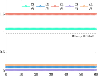
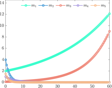
Figure 2: Left to right: evolution in time of number of agents (divided by $\rho_{i}^{c}$ and average viral load, in absence of mobility ($\chi=0$). We see that, in those nodes where the initial mass fraction $\rho_{i}$ is greater than the associated critical value $\rho_{i}^{c}$, the average viral load grows exponentially, while in the other nodes vanishes. Refer to Section 5.2 for additional details about the simulation.

On the other hand, if there is migration on the graph, we anyway have that, as a consequence of (2), the variation of the total average on the graph is only due to the interactions inside the nodes, as

$$\frac{d}{dt}\sum_{i\in\mathcal{I}}\rho_{i}m_{i}=\sigma\sum_{i\in\mathcal{I}}\rho_{i}m_{i}(\sigma\nu_{2}^{i}\rho_{i}-\gamma\nu_{1}^{i}).$$ (57)

As a consequence, again, it is possible to prove by means of a linear stability analysis that

Proposition 17.

Assume the graph is strongly connected. When $t\rightarrow\infty$

1. If $\rho_{i}^{\infty}<\rho_{i}^{c},\,\forall i$ then the solution $m_{i}$ of (64) $m_{i}\rightarrow 0$ for all $i\in\mathcal{I}$;

2. $\gamma\nu_{1}^{i}>\sigma\nu_{2}^{i}$, i.e., $\rho_{i}^{c}>1$, then $m_{i}\rightarrow 0$ for all $i\in\mathcal{I}$;

3. If $\rho_{i}^{c}<\rho_{m}^{\infty}\coloneqq\displaystyle\min_{i\in\mathcal{I}}\rho_{i}^{\infty}$ for all $i\in\mathcal{I}$ then the solution $m_{i}$ of (64) $m_{i}\rightarrow\infty$ for some $i\in\mathcal{I}$;

Proof.

We are interested in the stability of the asymptotic state $\bm{m}^{\infty}=0$ which represents the eradication of the infection in all nodes of the network. Linearising equation (57) around the equilibrium configuration $(\bm{\rho},\bm{m})=(\bm{\rho}^{\infty},\bm{0})$, we obtain

$$\frac{d}{dt}\sum_{i\in\mathcal{I}}\rho_{i}^{\infty}m_{i}=\sum_{i\in\mathcal{I}}\rho_{i}^{\infty}m_{i}(\sigma\nu_{2}^{i}\rho_{i}^{\infty}-\gamma\nu_{1}^{i}).$$ (58)

If $\rho_{i}^{\infty}<\rho_{i}^{c}\,\forall i\in\mathcal{I}$, then setting $d\coloneqq\displaystyle\max_{i\in\mathcal{I}}\left(\sigma\nu_{2}^{i}\rho_{i}^{\infty}-\gamma\nu_{1}^{i}\right)$, we have that

$$\frac{d}{dt}\sum_{i\in\mathcal{I}}\rho_{i}^{\infty}m_{i}\leq d\sum_{i\in\mathcal{I}}\rho_{i}^{\infty}m_{i}$$

and $m_{i}\rightarrow 0$ as $d\leq 0$. This proves the point 1 of the Proposition. Moreover, as $\rho_{i}^{\infty}\leq 1$, we have that

$$\frac{d}{dt}\sum_{i\in\mathcal{I}}\rho_{i}^{\infty}m_{i}\leq\sum_{i\in\mathcal{I}}\rho_{i}^{\infty}m_{i}(\sigma\nu_{2}^{i}-\gamma\nu_{1}^{i})$$ (59)

then, if $\sigma\nu_{2}^{i}-\gamma\nu_{1}^{i}<0\,\forall i$, we can conclude again that $m_{i}\rightarrow 0$. This proves point 2. Conversely, if $\rho_{i}^{c}<\rho_{m}^{\infty}\coloneqq\min\rho_{i}^{\infty}$, then

$$\frac{d}{dt}\sum_{i\in\mathcal{I}}\rho_{i}^{\infty}m_{i}\geq\sum_{i\in\mathcal{I}}\rho_{i}^{\infty}m_{i}b$$ (60)

where $b\coloneqq\displaystyle\min_{i\in\mathcal{I}}\left(\sigma\nu_{2}^{i}\rho_{m}^{\infty}-\gamma\nu_{1}^{i}\right)$ that is a positive quantity. In conclusion, $\exists i\in\mathcal{I}$ such that $m_{i}\rightarrow\infty$. ∎

Remark 18.

Notice that, if $\rho_{i}^{c}>1$ then $m_{i}\rightarrow 0$ (case 2). If $\rho_{i}^{c}<1$ then if Case 1 holds then there is eradication, while if Case 3 holds then there is blow up.

Remark 19.

We do not consider the case of constant infection/healing coefficients, as now, also in the linearised case, the infection coefficient always depends on the node through $\rho_{i}^{\infty}$.

Remark 20.

Notice that this dynamics is influenced by the values of $\rho_{i}^{\infty},\rho_{i}^{c},\sigma\nu_{2}^{i},\gamma\nu_{1}^{i}$, but, also by $\rho_{i}(0)$ and the migration strategy defined by $P_{ij}$ and $\chi$. For this reason, the values of the averages $m_{i}$ may also oscillate in some parameters regimes. Specifically, we may consider the following cases:

• when $\sigma\nu_{2}^{i}\leq\gamma\nu_{1}^{i}\,\forall i\in\mathcal{I}$, then $m_{i}\rightarrow 0$ $\forall i\in\mathcal{I}$, as this corresponds to $\rho_{i}^{c}\geq 1\geq\rho_{i}^{\infty},\,\forall i\in\mathcal{I}$;

• when $\sigma\nu_{2}^{i}>\gamma\nu_{1}^{i}$ for some $i$, then we have that, according to the value of $\rho_{i}(t)$ with respect to $\rho^{c}_{i}$, the evolution of the average may invert its trend. In fact, when $\rho_{i}(t)>\rho_{i}^{c}$, then $\sigma\nu_{2}^{i}\rho_{i}(t)-\gamma\nu_{1}^{i}>0$, and then the contribution of the exchange process to $m_{i}$ ($\left[\frac{d}{dt}m_{i}\right]_{\sigma}+\left[\frac{d}{dt}m_{i}\right]_{\gamma}$) is positive, while when $\rho_{i}(t)<\rho^{c}$, then $\sigma\nu_{2}^{i}\rho_{i}(t)-\gamma\nu_{1}^{i}<0$ and this contribution is negative. In particular, we can argue that, given an initial condition $\rho_{i}(0)$ in each node and the corresponding stationary state $\rho_{i}^{\infty}$, then, if

  $$(\rho_{i}(0)-\rho_{i}^{c})(\rho_{i}^{\infty}-\rho_{i}^{c})<0$$

  then there exists $\bar{t}$ such that $\rho_{i}(\bar{t})=\rho_{i}^{c}$. Then, if $\rho_{i}(0)>\rho_{i}^{c}$, then $m_{i}\rightarrow 0$, else if $\rho_{i}(0)<\rho_{i}^{c}$, then $m_{i}\rightarrow\infty$. Conversely, when

  $$(\rho_{i}(0)-\rho_{i}^{c})(\rho_{i}^{\infty}-\rho_{i}^{c})>0$$

  then, if $\rho_{i}^{\infty},\rho_{i}(0)<\rho_{i}^{c}$ then $m_{i}\rightarrow\infty$. Else, if $\rho_{i}^{\infty},\rho_{i}(0)>\rho_{i}^{c}$, then $m_{i}\rightarrow 0$.

4.3 Control in each node

We now implement two independent controls on the migration dynamics and on the binary interactions leading to infection. We, then, define the controlled problem as

$$\frac{d}{dt}\int_{\mathbb{R}_{+}}\varphi(v)f_{i}(v,t)\,dv =\sigma_{i}\int_{{\mathbb{R}_{+}}}\varphi(v)Q^{+}(f_{i},f_{i})(v,t)\,dv+\gamma\int_{{\mathbb{R}_{+}}}\varphi(v)Q^{-}(f_{i})(v,t)\,dv,$$ (61)

$$\hphantom{{}=}+\chi\int_{\mathbb{R}_{+}}\varphi(v)\bigl{[}\sum_{j\in\mathcal{I}}P_{ij}^{u}f_{j}(t,v)-f_{i}(t,v)\bigr{]}\,dv,$$

where the control matrix $P_{ij}^{u}$ is defined by equation (19), while the control $\sigma_{i}$ on the binary interactions is defined by

$$\sigma_{i}:=\sigma(1-u_{i}^{\sigma})$$ (62)

and has the effect of reducing the infection rate inside each node.

Concerning the controlled macroscopic equations, we have that the evolution of the masses is again given by (39), while setting $\varphi=v$ in (61) we obtain for the controlled weighted average $\rho_{i}^{u}m_{i}^{u}$

$$\frac{d}{dt}\rho_{i}^{u}(t)m_{i}^{u}(t)=\chi\biggl{[}\sum_{j\in\mathcal{I}}P_{ij}^{u}\rho_{j}^{u}(t)m_{j}^{u}(t)-\rho_{i}^{u}(t)m_{i}^{u}(t)\biggr{]}+\sigma(1-u_{i}^{\sigma})\nu^{i}_{2}\rho_{i}^{u^{2}}(t)m_{i}^{u}(t)-\gamma\nu^{i}_{1}\rho_{i}^{u}(t)m_{i}^{u}(t),$$ (63)

and, also

$$\frac{d}{dt}m_{i}^{u}(t)=\chi\biggl{[}\sum_{\begin{subarray}{c}j\in\mathcal{I}\\ j\neq i\end{subarray}}P_{ij}^{u}\frac{\rho_{j}^{u}(t)}{\rho_{i}^{u}(t)}\bigl{(}m_{j}^{u}(t)-m_{i}^{u}(t)\bigr{)}\biggr{]}+\sigma(1-u_{i}^{\sigma})\nu^{i}_{2}\rho_{i}^{u}(t)m_{i}^{u}(t)-\gamma\nu^{i}_{1}m_{i}^{u}(t),$$ (64)

i.e.

$$\frac{d}{dt}m_{i}^{u}=(1-u_{i}^{\chi})\left[\frac{d}{dt}m_{i}\right]_{\chi}+(1-u_{i}^{\sigma})\left[\frac{d}{dt}m_{i}\right]_{\sigma}-\left[\frac{d}{dt}m_{i}\right]_{\gamma},$$

where in the right hand side the quantities are defined in (13)-(55).

Remark 21.

Again, we can remark that for both the evolution of the masses and of the averages, the controls $1-u_{i}^{\chi},1-u_{i}^{\sigma}\in[0,1]$ reduce the time variation rate, without inverting the natural trend, with $u_{i}^{\sigma},u_{i}^{\chi}=1$ stopping the time evolution. The difference here is that when increasing $u_{i}^{\sigma}$, the effect of $-\left[\frac{d}{dt}m_{i}\right]_{\gamma}$ is stronger.

4.4 Optimality conditions

From now on, we drop the apex ^u on the average quantities $\rho_{i},\rho_{i}m_{i}$ of the controlled problem. We now want to find the optimal control $\bar{u}_{i}^{\sigma},\bar{u}_{i}^{\chi}$, as done in the previous section. Let us then consider the problem with a discretisation in time

$$\int_{\mathbb{R}_{+}}\varphi(v)f_{i}(t+h,v)\,dv =\int_{\mathbb{R}_{+}}\varphi(v)f_{i}(t,v)\,dv+h\chi\int_{\mathbb{R}_{+}}\varphi(v)\bigl{[}\sum_{j\in\mathcal{I}}P_{ij}^{u}f_{i}(t,v)-f_{i}(t,v)\bigr{]}\,dv$$ (65)

$${\hphantom{{}={}}}+h\sigma(1-u_{i}^{\sigma})\,\left\langle\int_{\mathbb{R}_{+}}\!\int_{\mathbb{R}_{+}}(\varphi(v^{\prime})-\varphi(v))f_{i}(t,v)f_{i}(t,v_{*})\,dv_{*}\,dv\right\rangle$$

$${\hphantom{{}={}}}-h\gamma\int_{{\mathbb{R}_{+}}}\!\langle\varphi(v^{\prime\prime})-\varphi(v)\rangle f_{i}(v,t)\,dv.$$

We consider again the cost functional aiming at minimising the average weighted by the mass in each node $\rho_{i}m_{i}$

$$\mathcal{J}_{h}^{i}(u_{i}^{\chi},u_{i}^{\sigma},\rho_{i}m_{i})=\psi(\rho_{i}m_{i}(t+h))+\frac{1}{2}\nu^{\chi}{u_{i}^{\chi}}^{2}+\frac{1}{2}\nu^{\sigma}{u_{i}^{\sigma}}^{2},$$ (66)

The minimisation conditions are

$$D_{u_{i}^{\chi}}\mathcal{J}_{h}^{i}(u_{i}^{\chi},u_{i}^{\sigma},\rho_{i}m_{i})=0,\qquad D_{u_{i}^{\sigma}}\mathcal{J}_{h}^{i}(u_{i}^{\chi},u_{i}^{\sigma},\rho_{i}m_{i})=0,$$

that imply

$$\frac{d\rho_{i}m_{i}}{du_{i}^{\chi}}\psi^{\prime}(\rho_{i}m_{i}(t+h))+\nu^{\chi}u_{i}^{\chi}=0,\qquad\frac{d\rho_{i}m_{i}}{du_{i}^{\mu}}\psi^{\prime}(\rho_{i}m_{i}(t+h))+\nu^{\sigma}u_{i}^{\sigma}=0,$$

that, from equation (64), is equivalent to

$$\nu^{\chi}u_{i}^{\chi}+\psi^{\prime}(\rho_{i}m_{i}(t+h))h\left[-\chi\left(\sum_{j}P_{ij}\rho_{j}m_{j}-\rho_{i}m_{i}\right)\right]=0,\qquad\nu^{\sigma}u_{i}^{\sigma}+\psi^{\prime}(\rho_{i}m_{i}(t+h))h\left[\sigma\nu_{2}^{i}\rho_{i}^{2}m_{i}\right]=0.$$

Now, if we impose $\nu^{\alpha}=hk^{\alpha},\,\alpha=\chi,\sigma$ for suitable $k_{i}^{\chi},k_{i}^{\sigma}>0$, we can write

$$\bar{u}_{i}^{\chi}(t+h)=\psi^{\prime}(\rho_{i}m_{i}(t+h))\biggl{[}\frac{\chi}{k_{i}^{\chi}}\left(\sum_{j}P_{ij}\rho_{j}m_{j}-\rho_{i}m_{i}\right)\biggr{]},\qquad\bar{u}_{i}^{\sigma}(t+h)=\psi^{\prime}(\rho_{i}m_{i}(t+h))\biggl{[}\frac{\sigma}{k_{i}^{\sigma}}\nu^{i}_{2}\rho_{i}^{2}m_{i}\biggr{]}.$$ (67)

Then, when $h\to 0$ in equation (65), we have

$$u_{i}^{\chi}=\min\{\max\{\delta,\bar{u}_{i}^{\chi}\},1\},\qquad u_{i}^{\sigma}=\min\{\max\{0,\bar{u}_{i}^{\sigma}\},1\}$$ (68)

with $\delta>0$ being the minimum entry of $P_{ij}$ and

$$\bar{u}_{i}^{\chi}(t)=\psi^{\prime}(\rho_{i}m_{i}(t))\left[\dfrac{\chi}{k_{i}^{\chi}}(\sum_{j}P_{ij}\rho_{j}m_{j}-\rho_{i}m_{i})\right],\qquad\bar{u}_{i}^{\sigma}(t)=\psi^{\prime}(\rho_{i}m_{i}(t))\left[\dfrac{\sigma}{k_{i}^{\sigma}}\nu_{2}^{i}\rho_{i}^{2}m_{i}\right].$$ (69)

Now, we discuss the compatibility of $\bar{u}_{i}^{\sigma}$, considering, again $\psi$ given by (32). Then, imposing that $\bar{u}_{i}^{\sigma}\leq 1$, we find

$$k_{i}^{\sigma}\geq\rho_{i}^{q+1}(t)m_{i}^{q}(t)\nu_{2}^{i}\sigma.$$ (70)

However, now, we also impose that

$$\sigma(1-u_{i}^{\sigma})\nu_{2}^{i}<\gamma\nu_{1}^{i},$$

because in this way we choose a control that is strong enough in order to make the binary interaction process weaker than the healing one in each node. The latter is satisfied if

$$\bar{u}_{i}^{\sigma}\geq 1-\rho_{i}^{c}.$$ (71)

Of course, the latter makes sense only in the case $\rho_{i}^{c}<1$ that is also the dangerous one. We have that (71) holds true choosing

$$k_{i}^{\sigma}\leq\frac{\rho_{i}^{q+1}(t)m_{i}(t)^{q}\nu_{2}^{i}\sigma}{1-\rho_{i}^{c}}$$ (72)

Therefore

$$k_{i}^{\sigma}(t)\in\biggl{[}\rho_{i}^{q+1}(t)m_{i}^{q}(t)\nu_{2}^{i}\sigma,\frac{\rho_{i}^{q+1}(t)m_{i}^{q}(t)\nu_{2}^{i}\sigma}{1-\rho_{i}^{c}}\biggr{]},$$ (73)

that is well defined as $\rho_{i}^{c}<1$ required by (71).

Remark 22.

Differently with respect to Section 3.3, we require (70) instead of $k_{i}^{\sigma}\geq\rho_{i}^{q+1}(t)m_{i}(0)^{q}\nu_{2}^{i}\sigma$. This choice is linked to the necessity of having a good definition of the latter interval (73) of $k_{i}^{\sigma}$. This also leads to the fact that the penalisation coefficient now depends on time. Specifically for the choice $k_{i}^{\sigma}=\frac{\rho_{i}^{q+1}(t)m_{i}^{q}(t)\nu_{2}^{i}\sigma}{1-\rho_{i}^{c}}$, i.e., the upper bound of the interval, this is reasonable, as if the trend of the average $m_{i}$ is decreasing then restrictions can be made lighter: this corresponds to having a lower penalisation coefficient in such a way that a too high control is not applied.

4.5 Aggregate trend of the controlled problem

The macroscopic quantities then evolve as (39), (63) (or (64)) with the controls defined by (68), (69) with (33), (73). Again, in order to study the (at least linear) stability of possible stationary states $(\bm{\rho}^{\infty},\bm{0})$ we need to analyse the possibility of having a stationary transition probability. The latter amounts to investigating if the control on the mobility reaches a stationary state, i.e.

$$\lim_{t\rightarrow\infty}u_{i}^{\chi}(t)=u_{i}^{\chi,\infty}$$

and, then, if $\rho_{i}m_{i}$ tends in time to a stationary finite value $\rho_{i}^{\infty}m_{i}^{\infty}$. We consider the following possible cases.

• When $\sigma\nu_{2}^{i}\leq\gamma\nu_{1}^{i}$ then we know that $\rho_{i}^{\infty}m_{i}^{\infty}=0$ $\forall i\in\mathcal{I}$.

• When $\sigma\nu_{2}^{i}>\gamma\nu_{1}^{i}$ then $u_{i}^{\sigma}$ is chosen, thanks to (73), in such a way that $\rho_{i}^{\infty}m_{i}^{\infty}\rightarrow 0$.

In conclusion, the latter quantity defines a stationary controlled transition matrix $\mathbf{P}^{u,\infty}$ that is also irreducible. Again, it is possible to have a stationary state $\bm{\rho}^{\infty}$ and Propositions 1 holds true. We can also prove the controlled version of Proposition 17.

Proposition 23.

Assume the graph is strongly connected. When $t\rightarrow\infty$ the solution of (63) with (68)-(69)-(33)-(72) satisfies

$$m_{i}\rightarrow 0,$$

for any value of $\rho_{i}^{c}$.

Proof.

If $\rho_{i}^{c}\geq 1$ for all $i\in\mathcal{I}$ then we already knew that for the non-controlled problem $m_{i}\rightarrow 0$ for all $i\in\mathcal{I}$. Now, for $\rho_{i}^{c}<1$ for all $i\in\mathcal{I}$ we have that then $m_{i}\rightarrow 0$ for all $i\in\mathcal{I}$ thanks to the choice of the control defined by (69)-(33)-(72). ∎

Remark 24.

The choice of controlling and minimising the weighted average $\rho_{i}m_{i}$ inside each node is again due to the fact that the observations of Section 3.3 and Section 3.3.1 can be shown to hold true also in the present case.

4.6 Basic reproduction number

In the same spirit as in [33], we can determine a basic reproduction number $\mathcal{R}_{0}\geq 0$, that is a quantity typically defined in compartmental models and that represents the mean number of secondary infections caused by a single infected individual in a population of susceptible individuals. Mathematically, this parameter is defined as the one discriminating between the (linear) stability (if $\mathcal{R}_{0}<1$) or instability (if $\mathcal{R}_{0}>1$) of the disease-free equilibrium (no infected individuals).

As done in [33], as we are dealing with a non-compartmental viral load-based model, we define $R_{0}$ exploiting the stability/instability of the asymptotic state $\bm{m}^{\infty}=\mathbf{0}$. We then linearise (53) around the equilibrium $(\bm{\rho},\,\bm{m})=(\bm{\rho}^{\infty},\,\mathbf{0})$. Writing

$$\rho_{i}=\rho^{\infty}_{i}+\epsilon\tilde{\rho}_{i},\qquad m_{i}=\epsilon\tilde{m}_{i},$$

where $\epsilon>0$ is a small parameter, and plugging into (53) we obtain, at the leading order in $\epsilon$, the following equations for the perturbations $\tilde{m}_{i}$:

$$\frac{d\tilde{m}_{i}}{dt}=\frac{\chi}{\rho^{\infty}_{i}}\sum_{j\in\mathcal{I}}P_{ij}\rho^{\infty}_{j}(\tilde{m}_{j}-\tilde{m}_{i})+\mu(\nu_{2}\rho^{\infty}_{i}-\nu_{1})\tilde{m}_{i},\qquad i\in\mathcal{I}.$$

We remark that we consider constant parameters $\nu_{2},\nu_{1}$ for simplicity. Introducing the diagonal matrix $\mathbf{R}:=\operatorname{diag}(\rho^{\infty}_{1},\,\dots,\,\rho^{\infty}_{n})$, this linear system may be rewritten in compact form as

$$\frac{d\tilde{\bm{m}}}{dt}=\left[\chi\left(\mathbf{R}^{-1}\mathbf{P}\mathbf{R}-\mathbf{I}\right)+\sigma\nu_{2}\mathbf{R}-\gamma\nu_{1}\mathbf{I}\right]\tilde{\bm{m}},$$ (74)

where $\tilde{\bm{m}}:=(\tilde{m}_{1},\,\dots,\,\tilde{m}_{n})$, whence we deduce that the stability of the asymptotic state $\bm{m}^{\infty}=\mathbf{0}$ depends on the spectral properties of the matrix

$$\mathbf{A}:=\chi\left(\mathbf{R}^{-1}\mathbf{P}\mathbf{R}-\mathbf{I}\right)+\sigma\nu_{2}\mathbf{R}-\gamma\nu_{1}\mathbf{I}\in\mathbb{R}^{n\times n}.$$

Remark that $\mathbf{A}$ has the form $\mathbf{A}=\mathbf{B}-\mathbf{D}$ with

$$\mathbf{B}:=\chi\mathbf{R}^{-1}\mathbf{P}\mathbf{R}+\mu\nu_{2}\mathbf{R}\in\mathbb{R}^{n\times n},\qquad\mathbf{D}:=\chi\mathbf{I}+\gamma\nu_{1}\mathbf{I}\in\mathbb{R}^{n\times n},$$

where $\mathbf{B}$, $\mathbf{D}$ are both non-negative and $\mathbf{D}$ is diagonal and invertible (at least for either $\chi>0$ or $\gamma\nu_{1}>0$). The Perron-Frobenius theory allows to state that $\tilde{\bm{m}}=\mathbf{0}$ is a stable equilibrium of (74) if and only if the spectral radius of the matrix $\mathbf{B}\mathbf{D}^{-1}$ is smaller than $1$. Conversely, if such a spectral radius is larger than $1$ then $\tilde{\bm{m}}=\mathbf{0}$ and $\bm{m}^{\infty}=\mathbf{0}$ are unstable.

Let $\beta_{ij}\in\mathbb{R}$ be the $ij$-entry of the matrix $\mathbf{B}\mathbf{D}^{-1}$, then:

$$\beta_{ij}:=\sum_{k=1}^{n}\mathbf{B}_{ik}\mathbf{D}^{-1}_{kj}=\frac{\chi P_{ij}\rho^{\infty}_{j}}{\chi\rho_{i}^{\infty}+\gamma\nu_{1}\rho_{i}^{\infty}}+\dfrac{\sigma\nu_{2}\rho_{i}^{\infty}}{\chi+\gamma\nu_{1}}\delta_{ij}$$

and, using, from the Perron-Frobenius Theorem,

$$\min_{i=1,\,\dots,\,n}\sum_{j=1}^{n}\beta_{ij}\leq\mathcal{R}_{0}\leq\max_{i=1,\,\dots,\,n}\sum_{j=1}^{n}\beta_{ij},$$ (75)

we have that

$$\dfrac{\chi+\sigma\nu_{2}\rho_{m}^{\infty}}{\chi+\gamma\nu_{1}}\leq\mathcal{R}_{0}\leq\dfrac{\chi+\sigma\nu_{2}\rho_{M}^{\infty}}{\chi+\gamma\nu_{1}}$$ (76)

being $\rho_{m}^{\infty}=\min_{i\in\mathcal{I}}\rho_{i}^{\infty}$ and $\rho_{M}^{\infty}=\max_{i\in\mathcal{I}}\rho_{i}^{\infty}$. We can also determine the basic reproduction number in the controlled case, and using the same estimation we find

$$\min_{i\in\mathcal{I}}\dfrac{\chi(1-u_{i}^{\chi,\infty})+\sigma(1-u_{i}^{\sigma,\infty})\nu_{2}\rho_{i}^{\infty}}{\chi(1-u_{i}^{\chi,\infty})+\gamma\nu_{1}}\leq\mathcal{R}_{0}\leq\displaystyle\max_{i\in\mathcal{I}}\dfrac{\chi(1-u_{i}^{\chi,\infty})+(1-u_{i}^{\sigma,\infty})\sigma\nu_{2}\rho_{i}^{\infty}}{\chi(1-u_{i}^{\chi,\infty})+\gamma\nu_{1}}.$$ (77)

5 Numerical experiments

In this section, we present several results from numerical experiments on the models previously discussed. In particular, we structure the presentation in three parts:

1. Firstly, we show different aggregate trends arising from the most basic type of interactions on graph, both in presence and absence of different control strategies. The equations we are referencing are (7), (10) and (39), (24), with control choices given by equations (30)–(34).

2. Next, we consider the descriptions gathering together infection and healing, again in both the controlled and the uncontrolled case. This time, the equations we focus on are (7), (52) and (39), (63), with control choices given by equations (68), (69) and (33)-(73), choosing the lowest value for the penalisation coefficient. Finally, we use (76),(77) to estimate the basic reproduction number.

3. We conclude the section by applying the infection-healing model to a real-world mobility scenario, employing recent census data on the northern Italy region of Lombardy.

All the aforementioned macroscopic equations are solved via standard numerical methods for systems of ordinary differential equations, such as the classical fourth-order Runge-Kutta method. We always consider a fully connected graph with $N=5$ nodes. Unless otherwise specified, we set the parameters reported in Table 1 for all the numerical tests.

$\displaystyle\mathbf{P}=\left(\begin{array}[]{*{5}{l}}0.2&0.5&0.15&0.1&0.1\\ 0.2&0.2&0.45&0.4&0.2\\ 0.2&0.1&0.05&0.2&0.5\\ 0.2&0.1&0.1&0.15&0.1\\ 0.2&0.1&0.25&0.15&0.1\end{array}\right),\quad\bm{\rho}(t=0)=\left(\begin{array}[]{l}0.35\\ 0.1\\ 0.3\\ 0.05\\ 0.2\end{array}\right),\quad\bm{m}(t=0)=\left(\begin{array}[]{l}2\\ 4\\ 0.1\\ 1\\ 1.5\end{array}\right),$ $N=5,\quad q=2,\quad\chi=1.$

Table 1: Parameters and initial conditions common to all tests in Section 5.1–5.2, unless otherwise specified.

5.1 Test 1: infection dynamics only

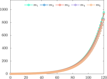
Figure 3: Evolution in time of number of agents (left) and average viral load (right): uncontrolled case. The infection grows exponentially on the graph.

We begin with the basic model described in Section 2 along with its controlled version described in Section 3. We present five different evolution scenarios, depending on the control strategy in force

1. No control: this is our reference, in order to compare the effects of different intervention policies (Figure 3).

2. Control on mobility only: we set $u_{i}^{\chi}(t)$ according to equation (30) but we set $u_{i}^{\mu}(t)=0$ for all $t\geq 0$ (Figure 4, top row).

3. Mobility suppression: we set $u_{i}^{\chi}(t)=1$ for all $t\geq 0$. This behavior mimics the effects of an enforced, total quarantine over the entire network. No control is set on the infection dynamics (Figure 4, bottom row).

4. Short-term intervention on interactions: both dynamics are controlled until the evolution time reaches a threshold value $t=\bar{t}$, after which, control on interactions is suspended, i.e., $u_{i}^{\mu}(t)=0$ for all $t>\bar{t}$. In our test, we set $\bar{t}=30$ (Figure 5, top row).

5. Full control: $u_{i}^{\chi}(t)$ and $u_{i}^{\mu}(t)$ are set according to (30) for all $t\geq 0$ (Figure 5, bottom row).

For all tests, we additionally set the following parameters:

$$\nu_{1}=(0.25,\,0.5,\,0.15,\,0.2,\,0.75)^{T},\quad\nu_{2}=(0.8,\,0.5,\,0.75,\,0.1,\,0.6)^{T},\quad\mu=1.$$ (78)

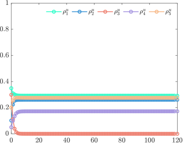
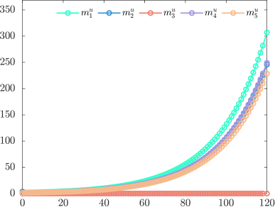
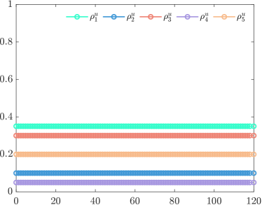
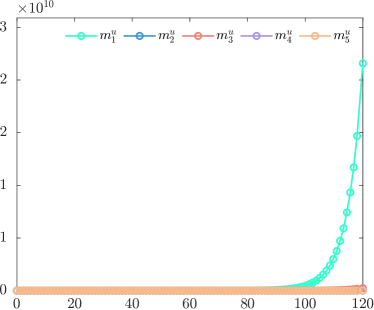
Figure 4: Columns: evolution in time of number of agents (left) and average viral load (right). Top row: effects of controlling the agents’ mobility alone. Agents leave node number 3 and distribute in the remaining vertices. The overall viral load is decreased by a factor of 3 with respect to the uncontrolled scenario. Bottom row: effects of node isolation. Without in-node interventions and preventing highly infectious agents to distribute in nodes with lower load, the infection can grow dramatically by several order of magnitudes.

Figure 3 shows the reference, uncontrolled case, where, at the end of the simulation period, the average viral load in each node reaches values near $10^{3}$. Intervening on just the mobility, rerouting infectious people, can be partially effective (see Figure 4, top row, exhibiting the average viral load reduced by a factor of 3); still, it is insufficient to prevent the growth of infection overall to satisfactory levels. As shown in Figure 4, bottom row, isolating nodes, without simultaneous in-node interventions, can not only be ineffective, but even cause more harm than good, as already remarked, e.g., in [20] and [33]. Indeed, in-node interventions, even if for just a shorter amount of time, have a high impact on the growth rate of the average viral load: controlling the in-node interactions for just the initial 25% of time is responsible for a nearly 33% decrease in the infection spread, as shown in Figure 5, top row.

Finally, the bottom row of Figure 5 shows the effectiveness of combining the control actions on both mobility and in-node interactions, enabling the infection spread to stop at a low average viral load value.

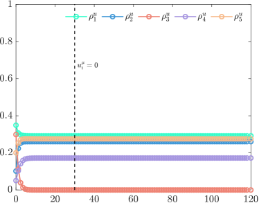
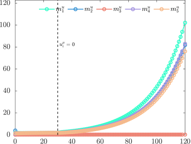
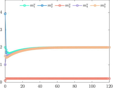
Figure 5: Columns: evolution in time of number of agents (left) and average viral load (right). Top row: effects of partial in-node interventions. Even if limited to the early stages of infection, when it is still spreading to a comparatively low levels, control policies that slow in-node interactions between agent have a meaningful impact when compared to interventions on the mobility alone, with a reduction of about 30% in the average viral load values. Bottom row: both in-node interactions and mobility are controlled fully. The infection ceases spreading after the average viral load reaching a value nearly three orders of magnitudes lower than the uncontrolled scenario.

5.2 Test 2: infection and healing dynamics altogether

Next, we focus on the model coupling the binary, in-node interaction dynamics with a healing process, described in Section 4. In this test, we compare the uncontrolled evolution of the infection with a fully controlled scenario, where we set $u_{i}^{\chi}$ and $u_{i}^{\sigma}$ as prescribed by equation (69). In particular, in addition to the parameters and data in Table 1, we also set

$$\nu_{1}^{i}=0.15,\qquad\nu_{2}^{i}=0.9,\quad\forall\,i\in\mathcal{I},\quad\sigma=1,\quad\gamma=1,$$ (79)

the exchange parameters being chosen in order to ensure that $m_{i}(t)\to+\infty$ in the uncontrolled case (see Proposition 23), so that we can have a sensible comparison of both dynamics.

In Figure 6 we report the results of the simulations: as expected, the healing process is capable alone to slow down the spread of the infection, which reaches lower values than the ones reported in its basic counterpart in Figure 3, even with exchanging coefficients $\nu_{1}^{i}$ and $\nu_{2}^{i}$ more prone to faster dissemination. Nevertheless, the top row shows that the average viral load still grows exponentially in the uncontrolled case. This is also testified by the upper bound for the basic reproduction number being greater than 1, computed as reported in equation (76).

The bottom row instead shows the effects of controlling both the mobility and the in-node interactions: controlling the latter has so much relative importance, in this example, that the evolution of the number of agents is barely affected and only in the initial stages of the simulation. On the other hand, the control strategy is highly effective on the contagion dynamics, as the average viral load vanishes rapidly, as testified again by the bounds for the basic reproduction number, both below the critical value 1. These results are in agreement with the computations presented in Section 4.

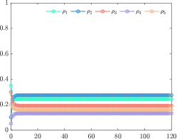
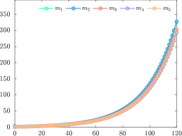
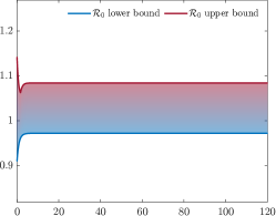
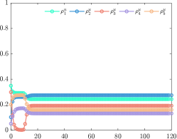
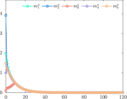
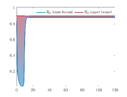
Figure 6: Columns, from left to right: evolution in time of the number of agents, average viral load and basic reproduction number bounds. Top row: uncontrolled case, as reference. Even if slower than the more basic model without healing, we still have exponential growth of the average viral load. Bottom row: effects of full control. Infection never starts and we see the system exponentially reaching a disease-free equilibrium.

5.3 Application to a real-world mobility scenario

We conclude the presentation of numerical experiments with an application to a real-world scenario. We chose to focus on data on mobility only for two reasons: first of all, even if we are presenting here models on agents exchanging viral load, the modeling framework is flexible enough to be oriented to different (or more general) binary interactions between agents on an underlying network, indeed being the graph and its associated transition matrix the critical components of our framework. Moreover, data on viral loads often present some degree of criticality (under-representation of low values of viral loads associated with little to no symptoms, lack of extensive testings in non-hospitalized patients, variable fitness of the carrying pathogen over time, …), making it extremely difficult to calibrate a multi-agent mathematical model on them (the interested reader may refer to e.g., [8] for a very recent data-driven approach with an underlying kinetic framework).

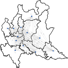
Figure 7: Fully connected, unweighted mobility network among all the provinces in Lombardy, Italy.

In order to keep the dataset relevant to our modeling setting (that is, a relatively large network, highly populated but still small enough to allow daily external mobility, so larger than a metropolitan area but smaller than a country) and also relevant for the recent SARS-CoV-2 pandemic, we chose data about the mobility habits of inhabitants of the region Lombardy, in northern Italy in 2016 (pre-pandemic). The spatial representation of the network is presented for reference in Figure 7. For what concerns the initial number of agents in each node, we considered the official country’s census data. The corresponding transition matrix and initial data and parameters are reported in Table 2.

$\displaystyle\mathbf{P}=\left(\begin{tabular}[]{colspec={S[table-format=1.4]S[table-format=1.4]S[table-format=1.4]S[table-format=1.4]S[table-format=1.4]S[table-format=1.4]S[table-format=1.4]S[table-format=1.4]S[table-format=1.4]S[table-format=1.4]S[table-format=1.4]S[table-format=1.4]}, colsep=1ex}0.8757873534506977&0.03526595143954377&$0.0054794387934947435$&0.02158985767625072&0.03736936844586586&$0.002\,302\,956\,167\,961\,513$&$0.011\,334\,416\,300\,349\,221$&$0.013\,701\,264\,437\,385\,683$&$0.002\,918\,347\,645\,093\,448\,2$&$0.002\,845\,914\,850\,987\,816$&$0.003\,648\,879\,922\,951\,077\,4$&$0.003\,205\,249\,781\,094\,776\,4$\\ 0.04635026989878317&0.9257936902391382&$0.0014357475896173866$&0.03174345308918152&0.002270751201990444&$0.003\,594\,862\,553\,021\,278$&$0.003\,661\,559\,967\,382\,806$&$0.005\,001\,453\,613\,941\,826\,5$&$0.034\,928\,299\,968\,198\,774$&$0.002\,278\,835\,850\,734\,442$&$0.003\,142\,724\,263\,924\,889\,7$&$0.002\,446\,923\,335\,611\,406$\\ 0.002295776667751961&0.0005129948376395526&$0.8154610223024258$&0.0006910638094203594&0.034635103119906446&$0.001\,548\,916\,939\,116\,723$&$0.032\,635\,884\,655\,101\,88$&$0.007\,767\,637\,575\,529\,528$&$0.000\,690\,052\,285\,791\,359\,9$&$0.001\,770\,585\,268\,528\,977\,8$&$0.015\,366\,268\,112\,956\,225$&$0.024\,656\,214\,415\,861\,424$\\ 0.007162945108250052&0.008473783507703942&$0.0005042923032038033$&0.8529198120471422&0.00044919089214553526&$0.041\,738\,089\,168\,026\,835$&$0.000\,848\,260\,867\,088\,444\,8$&$0.004\,101\,798\,820\,922\,688$&$0.018\,126\,970\,466\,792\,27$&$0.002\,174\,689\,338\,494\,364$&$0.000\,323\,554\,565\,104\,217\,75$&$0.000\,443\,345\,116\,395\,244\,1$\\ 0.010160987217152676&0.000519747424712148&$0.020542885462587812$&0.00042586302410433605&0.7816261016009323&$0.000\,572\,531\,720\,200\,114\,8$&$0.030\,398\,997\,670\,488\,94$&$0.003\,896\,024\,733\,430\,631\,4$&$0.000\,297\,791\,767\,031\,472\,95$&$0.000\,625\,907\,418\,301\,122\,7$&$0.016\,165\,127\,008\,202\,68$&$0.001\,264\,504\,244\,609\,959\,7$\\ 0.00044570353234450126&0.000573603881857499&$0.0005527865149536564$&0.023921110835510392&0.0004542106282002642&$0.745\,675\,156\,671\,644\,4$&$0.000\,413\,882\,256\,468\,270\,2$&$0.010\,470\,233\,241\,153\,605$&$0.000\,437\,094\,877\,688\,293\,96$&$0.012\,195\,850\,902\,711\,174$&$0.000\,270\,141\,321\,815\,319\,3$&$0.000\,731\,006\,671\,994\,478\,5$\\ 0.008474134237854567&0.0020595765975844737&$0.05198589677940409$&0.0018829004382285772&0.08172277492366109&$0.001\,237\,870\,447\,082\,813\,3$&$0.710\,460\,838\,570\,795\,3$&$0.044\,379\,804\,233\,793\,264$&$0.001\,309\,285\,834\,765\,772\,9$&$0.003\,271\,720\,543\,524\,3$&$0.002\,271\,165\,866\,704\,664$&$0.008\,437\,447\,792\,351\,163$\\ 0.0446185868510531&0.013123664706978934&$0.053052430159367024$&0.04106804676763683&0.047090653451488364&$0.171\,110\,490\,069\,136\,87$&$0.197\,807\,409\,456\,767\,1$&$0.867\,291\,736\,974\,090\,2$&$0.003\,598\,624\,785\,918\,315\,6$&$0.105\,633\,014\,285\,936\,81$&$0.004\,269\,616\,682\,098\,683$&$0.106\,454\,021\,051\,850\,95$\\ 0.0005365037466188645&0.010815293520094473&$0.000351684818746578$&0.02149587688610248&0.0001434776436996389&$0.000\,807\,480\,431\,655\,398\,5$&$0.000\,433\,342\,910\,556\,855\,8$&$0.000\,364\,515\,212\,356\,600\,3$&$0.934\,927\,589\,446\,492\,5$&$0.000\,903\,607\,810\,829\,709\,6$&$0.000\,231\,936\,480\,088\,653\,94$&$0.000\,533\,329\,795\,091\,531\,6$\\ 0.0012880928296168286&0.0008864002328547886&$0.0016211972361365747$&0.0028965791176721973&0.0009985689223157095&$0.027\,892\,767\,776\,822\,522$&$0.002\,062\,754\,282\,659\,092$&$0.015\,529\,675\,735\,539\,672$&$0.001\,119\,151\,970\,283\,140\,2$&$0.864\,778\,891\,848\,313\,1$&$0.000\,571\,969\,598\,973\,488\,9$&$0.001\,587\,329\,172\,944\,043$\\ 0.0005778134784514185&0.000459143073049482&$0.005893878831690055$&0.00018553162048871004&0.009780314082241892&$0.000\,202\,691\,408\,857\,945$&$0.000\,538\,729\,144\,537\,431\,8$&$0.000\,184\,736\,384\,801\,296\,12$&$0.000\,150\,070\,359\,888\,576\,1$&$0.000\,164\,747\,938\,667\,897\,9$&$0.952\,404\,622\,097\,292\,9$&$0.000\,285\,543\,364\,358\,950\,6$\\ 0.0023018329814251818&0.0015161505388427983&$0.04311873920837233$&0.0011799046882619878&0.003459485087552358&$0.003\,316\,186\,646\,473\,646$&$0.009\,403\,923\,917\,804\,436$&$0.027\,311\,119\,037\,054\,99$&$0.001\,496\,720\,592\,056\,120\,3$&$0.003\,356\,233\,942\,970\,127$&$0.001\,333\,994\,079\,887\,321\,2$&$0.849\,955\,085\,257\,836$\\ \end{tabular}\right)$,  $\displaystyle\bm{\rho}(t=0)=\left(\begin{tabular}[]{colspec={S[table-format=1.4]}, colsep=1ex}0.111429568301365\\ 0.126797034990562\\ 0.0361007484289710\\ 0.0601448912068948\\ 0.0340388722947419\\ 0.0229591510831975\\ 0.0870627833902669\\ 0.318267453990158\\ 0.0413704681415706\\ 0.0544775057762816\\ 0.0183028026195141\\ 0.0890487197764766\end{tabular}\right)$ $\displaystyle N=12,\quad m_{i}(t=0)=\begin{cases}1/6&\text{if }i\neq 6\\ 6&\text{otherwise}\end{cases},\qquad\nu_{1}^{i}=0.15,\qquad\nu_{2}^{i}=0.9,\quad\forall\,i\in\mathcal{I}$

Table 2: Parameters

In Figure 8 we report the results of the numerical experiment. We consider again the infection-healing modeling framework of Section 4, as we did in Section 5.2, but this time we consider much less restrictive in-node control actions. Indeed, we know from Proposition 23 that we can achieve eradication over the whole network if we set $u_{i}^{\sigma}(t)\geq 1-\rho_{i}^{c}$ for all $t\geq 0$. This, however, might imply a very high associated cost, especially in those cases when some nonzero viral load is present along the network but its value is still negligible.

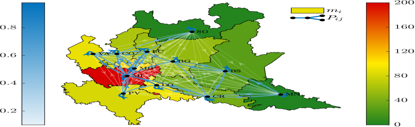
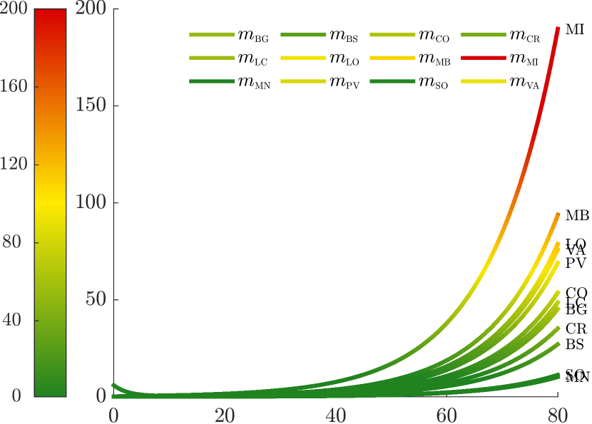
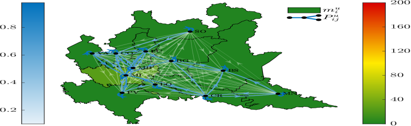
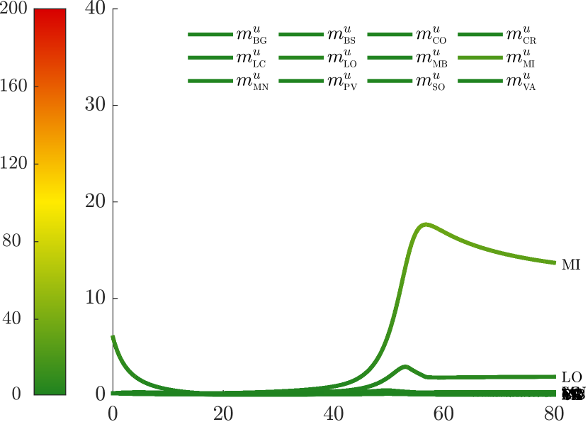
Figure 8: Columns, from left to right: heat-map of the infection state along the mobility network at the end of the simulation period; evolution in time of the average viral load on the network. Top row: uncontrolled scenario, as reference. We see exponential spread of the infection, at different rates. Bottom row: effects of light in-node control. Even if the control strength was not sufficient to achieve eradication across the network, the average viral load reaches values that are more than one order of magnitude lower than the reference case, thus obtaining a satisfactory result.

In the bottom row of Figure 8 we show that even if we do not achieve complete eradication, we still are able to lower the average viral load by more than one order of magnitude by relaxing the lower bound on $u_{i}^{\sigma}$ to be

$$u_{i}^{\sigma}(t)=\min(\max(0,\tilde{k}_{i}^{\sigma}\times 2.5\cdot 10^{-5}),1),\qquad\tilde{k}_{i}^{\sigma}=(\rho_{i}(0)m_{i}(0))^{q}\sigma\nu_{2}^{i},$$

with a substantial decrease in the associated penalization coefficient (and therefore its associated cost).

6 Conclusions

In the present work, we have proposed the optimal control of a kinetic model describing social interactions on a graph. The basic kinetic model, that was proposed in [33], describes agents migrating on the nodes of a graph and exchanging a physical quantity $v>0$ as a consequence of binary interactions. Here, the control aims at minimising the macroscopic average of the aforementioned physical quantity $v$. In [33], the kinetic model describes the spread of an infectious disease on a graph: as such, the positive quantity $v$ represents the viral-load of the potentially infected individual. The binary exchange rules are linear ones, and the exchange and migration mechanisms are stochastic independent. As a consequence, in the present work we have implemented two different controls on the two mechanisms in order to minimise the quantity related to the macroscopic average viral load. In order to do this we have applied the method used in [3]. Specifically, we have chosen to minimise the average $\rho_{i}m_{i}$ in each node weighted by the mass. In fact, we have shown that controlling $\rho_{i}m_{i}$ is effective as either controlling the mean $m_{i}$ in each node or controlling the global average $m$, but less expensive. This is due to the fact that implementing the same control everywhere (control on $m$), or controlling the same amount of mean viral-load $m_{i}$ regardless of the population quantity $\rho_{i}$, corresponds to exerting an excessive control for obtaining the same result. The best success that can be reached by this controlled model is to stop the increase of the infection, but eradication cannot be obtained, unless there are a priori natural conditions such as $\nu_{2}<\nu_{1}$. This is due to the interaction process, that includes the infection and healing within the same process.

As a consequence, we have proposed an adaptation of the model introduced in [33]. As the key point in the model proposed in [33] is that it prescribes simultaneous infection and healing within the same binary interaction rule, we have split the interaction into an infection process (due to a binary interaction) and a healing one (due to an autonomous process). Then, we have controlled only the migration and the infection processes. This has allowed to show that a sufficient control allows to reach eradication, even if the a priori conditions would not allow it.

Overall, the proposed controlled models allow to test the effect of each control strategy alone as well as the interplay of the simultaneous controlling strategies. This has allowed to obtain similar results that were obtained in previous studies [20], but also to highlight the drawbacks of the present control strategy, that prescribes a control that may be too high and persisting in time. This happens because of the choice (32) that aims at obtaining complete eradication ($m_{i}\rightarrow 0$). This reminds, for example, of the quarantine methods through PCR tests adopted during the COVID-19 pandemics: as the sensitivity of those tests was too high, then also recovered and not infectious individuals were isolated, because some viral load was still measured by the swab. Even though the PCR test and our control are different, because the first one is a microscopic (individual) control while the second one is a macroscopic (population level) control, this suggests, as a future perspective, that the control may be improved by adapting the cost function $\psi$ in order to demand that the average viral load is below a certain, even strictly positive, threshold, instead of requiring complete eradication. This may pose some challenges as $\psi^{\prime}$ could change sign instead of being always positive. Moreover, as a possible future work, we aim at integrating this viral-load modeling approach with a compartmental one, as done for example in [13, 15], but with control strategies on network.

We remark that we have presented the ‘less realistic’ model of Section 2, because it has allowed to introduce in [33] the concept of exchanging viral-load allowing to characterise the state of the individual with respect to the disease without considering the epidemic compartments. In the present work, it has allowed to face some difficulties in the definition of the control problem. Moreover, the simple linear interaction rules (3) of the model of Section 2 have proved to be effective in reproducing real phenomena of wealth exchange [12] and opinion exchange [44]. As a consequence, our framework could be adapted in order to consider the control in other phenomena of interest of social exchange on a graph or in presence of migrating subpopulations [6, 7].

References

• [1] G. Albi, L. Pareschi and M. Zanella “Boltzmann-type control of opinion consensus through leaders” In Philosophical Transactions of the Royal Society A: Mathematical, Physical and Engineering Sciences 372.2028, 2014, pp. 20140138
• [2] Giacomo Albi, Elisa Calzola and Giacomo Dimarco “A data-driven kinetic model for opinion dynamics with social network contacts” In European Journal of Applied Mathematics Cambridge University Press, 2024, pp. 1–27
• [3] Giacomo Albi, Lorenzo Pareschi and Mattia Zanella “Control with uncertain data of socially structured compartmental epidemic models” In Journal of Mathematical Biology 82 Springer, 2021, pp. 1–41
• [4] Marc Barthélemy and Alessandro Flammini “Optimal traffic networks” In Journal of Statistical Mechanics: Theory and Experiment 2006.07 IOP Publishing, 2006, pp. L07002
• [5] Giulia Bertaglia and Lorenzo Pareschi “Hyperbolic models for the spread of epidemics on networks: kinetic description and numerical methods” In ESAIM: M2AN 55.2, 2021, pp. 381–407
• [6] M. Bisi “Kinetic model for international trade allowing transfer of individuals” In Phil. Trans. A 380, 2022, pp. 20210156. (pp. 1–14)
• [7] M. Bisi and N. Loy “Kinetic models for systems of interacting agents with multiple microscopic states” In Physica D: Nonlinear Phenomena 457, 2024, pp. 133967
• [8] Andrea Bondesan, Antonio Piralla, Elena Ballante, Antonino Maria Guglielmo Pitrolo, Silvia Figini, Fausto Baldanti and Mattia Zanella “Predictability of viral load kinetics in the early phases of SARS-CoV-2 through a model-based approach” arXiv preprint arXiv:2407.03158, 2024
• [9] Alexandre Bovet and Hernán A Makse “Influence of fake news in Twitter during the 2016 US presidential election” In Nature communications 10.1 Nature Publishing Group UK London, 2019, pp. 7
• [10] Martin Burger “Network structured kinetic models of social interactions” In Vietnam Journal of Mathematics 49.3 Springer, 2021, pp. 937–956
• [11] C. Cercignani “The Boltzmann Equation and its Applications”, Applied Mathematical Sciences 67 New York: Springer, 1988
• [12] S. Cordier, L. Pareschi and G. Toscani “On a kinetic model for a simple market economy” In J. Stat. Phys. 120.1, 2005, pp. 253–277
• [13] R Della Marca, N Loy and M Menale “Intransigent vs. volatile opinions in a kinetic epidemic model with imitation game dynamics” In Press. In Mathematical Medicine and Biology, 2022
• [14] R Della Marca, N Loy and A Tosin “An SIR–like kinetic model tracking individuals’ viral load” In Networks and Heterogeneous Media 17.3, 2022, pp. 467–494
• [15] Rossella Della Marca, Nadia Loy and Andrea Tosin “An SIR–model with viral load-dependent transmission” In Journal of Mathematical Biology 86.4 Springer, 2023, pp. 61
• [16] G. Dimarco, G. Toscani and M. Zanella “Optimal control of epidemic spreading in the presence of social heterogeneity” In Philosophical Transactions of the Royal Society A: Mathematical, Physical and Engineering Sciences 380.2224, 2022, pp. 20210160
• [17] Giacomo Dimarco, Lorenzo Pareschi, Giuseppe Toscani and Mattia Zanella “Wealth distribution under the spread of infectious diseases” In Physical Review E 102 American Physical Society, 2020, pp. 022303
• [18] Bertram Düring, Jonathan Franceschi, Marie-Therese Wolfram and Mattia Zanella “Breaking consensus in kinetic opinion formation models on graphons” In Journal of Nonlinear Science 34.4 Springer, 2024, pp. 79
• [19] Amine El Bhih, Rachid Ghazzali, Soukaina Ben Rhila, Mostafa Rachik and Adil El Alami Laaroussi “A discrete mathematical modeling and optimal control of the rumor propagation in online social network” In Discrete dynamics in nature and society 2020.1 Wiley Online Library, 2020, pp. 4386476
• [20] Baltazar Espinoza, Carlos Castillo-Chavez and Charles Perrings “Mobility restrictions for the control of epidemics: When do they work?” In Plos one 15.7 Public Library of Science San Francisco, CA USA, 2020, pp. e0235731
• [21] Jonathan Franceschi, Andrea Medaglia and Mattia Zanella “On the optimal control of kinetic epidemic models with uncertain social features” In Optimal Control Applications and Methods 45.2 Wiley Online Library, 2023, pp. 494–522
• [22] Sonja Haug “Migration networks and migration decision-making” In Journal of ethnic and migration studies 34.4 Taylor & Francis, 2008, pp. 585–605
• [23] James A Hay, Lee Kennedy-Shaffer, Sanjat Kanjilal, Niall J Lennon, Stacey B Gabriel, Marc Lipsitch and Michael J Mina “Estimating epidemiologic dynamics from cross-sectional viral load distributions” In Science 373.6552 American Association for the Advancement of Science, 2021, pp. eabh0635
• [24] Kundan Kandhway and Joy Kuri “Using Node Centrality and Optimal Control to Maximize Information Diffusion in Social Networks” In IEEE Transactions on Systems, Man, and Cybernetics: Systems 47.7, 2017, pp. 1099–1110
• [25] Colleen F Kelley, Jason D Barbour and Frederick M Hecht “The relation between symptoms, viral load, and viral load set point in primary HIV infection” In JAIDS Journal of Acquired Immune Deficiency Syndromes 45.4 LWW, 2007, pp. 445–448
• [26] MHR Khouzani, Saswati Sarkar and Eitan Altman “Optimal control of epidemic evolution” In 2011 Proceedings IEEE INFOCOM, 2011, pp. 1683–1691 IEEE
• [27] Bactrin M Killingo, Trisa B Taro and Wame N Mosime “Community-driven demand creation for the use of routine viral load testing: a model to scale up routine viral load testing” In Journal of the International AIDS Society 20 Wiley Online Library, 2017, pp. e25009
• [28] István Z Kiss, Joel C Miller and Péter L Simon “Mathematics of epidemics on networks” In Cham: Springer 598.2017 Springer, 2017, pp. 31
• [29] Bichitra Kumar Lenka and Swaroop Nandan Bora “Metzler asymptotic stability of initial time linear time-varying real-order systems” In Franklin Open 4, 2023, pp. 100025
• [30] Kezan Li, Guanghu Zhu, Zhongjun Ma and Lijuan Chen “Dynamic stability of an SIQS epidemic network and its optimal control” In Communications in Nonlinear Science and Numerical Simulation 66 Elsevier, 2019, pp. 84–95
• [31] Fangzhou Liu and Martin Buss “Optimal control for heterogeneous node-based information epidemics over social networks” In IEEE Transactions on Control of Network Systems 7.3 IEEE, 2020, pp. 1115–1126
• [32] N. Loy and A. Tosin “Boltzmann–type equations for multi–agent systems with label switching” In Kinetic and Related Models 14.5, 2021, pp. 867–894
• [33] Nadia Loy and Andrea Tosin “A viral load-based model for epidemic spread on spatial networks” In Mathematical Biosciences and Engineering 18.5, 2021, pp. 5635–5663
• [34] Henryk Minc “Nonnegative matrices” Wiley New York, 1988
• [35] Yamir Moreno, Maziar Nekovee and Amalio F Pacheco “Dynamics of rumor spreading in complex networks” In Physical Review E—Statistical, Nonlinear, and Soft Matter Physics 69.6 APS, 2004, pp. 066130
• [36] Mark Newman “Networks” Oxford university press, 2018
• [37] Marco Nurisso, Matteo Raviola and Andrea Tosin “Network-based kinetic models: Emergence of a statistical description of the graph topology” In European Journal of Applied Mathematics Cambridge University Press, 2024, pp. 1–22
• [38] Markos Papageorgiou “Dynamic modeling, assignment, and route guidance in traffic networks” In Transportation Research Part B: Methodological 24.6 Elsevier, 1990, pp. 471–495
• [39] L. Pareschi and G. Toscani “Interacting Multiagent Systems: Kinetic equations and Monte Carlo methods” Oxford: Oxford University Press, 2013
• [40] Romualdo Pastor-Satorras, Claudio Castellano, Piet Van Mieghem and Alessandro Vespignani “Epidemic processes in complex networks” In Reviews of modern physics 87.3 APS, 2015, pp. 925–979
• [41] Stephen M Petrie, Teagan Guarnaccia, Karen L Laurie, Aeron C Hurt, Jodie McVernon and James M McCaw “Reducing uncertainty in within-host parameter estimates of influenza infection by measuring both infectious and total viral load” In PLoS One 8.5 Public Library of Science San Francisco, USA, 2013, pp. e64098
• [42] Sandip Roy, Terry F McElwain and Yan Wan “A network control theory approach to modeling and optimal control of zoonoses: case study of brucellosis transmission in sub-Saharan Africa” In PLoS neglected tropical diseases 5.10 Public Library of Science San Francisco, USA, 2011, pp. e1259
• [43] Caz M Taylor and D Ryan Norris “Population dynamics in migratory networks” In Theoretical Ecology 3 Springer, 2010, pp. 65–73
• [44] G. Toscani “Kinetic models of opinion formation” In Commun. Math. Sci. 4.3, 2006, pp. 481–496