Assessing Uncertainties in Parton Showers at Double Logarithmic Accuracy for Jet Quenching Studies

Abstract

This paper assesses the uncertainties inherent to parton shower simulations at double logarithmic accuracy, with a focus on their impact on jet quenching studies in high-energy heavy-ion collisions. For that purpose, we developed a massless quark-initiated vacuum parton shower toy-model with different evolution variables, such as inverse formation time, invariant squared mass, and squared opening angle. In addition to the effects of varying the ordering variable we further examine their corresponding kinematic reconstructions. The results highlight how these variations influence key distributions, including the number of splittings, angular and transverse momentum distribution of subsequent emissions. We also analyse the Lund distributions and their average trajectories, revealing that the choice of ordering variable has a significantly greater impact on the vacuum parton shower evolution than the kinematic scheme, particularly in large-angle emission regions. When a simple jet quenching model based on decoherence is implemented, we observe that the fraction of quenched events is sensitive to the ordering prescription, especially for the first splitting and thin media, highlighting the need for a deeper understanding of the branching process in the presence of an extended QCD media.

1 Introduction

The simulation of the branching process of a parton in Quantum Chromodynamics (QCD), i.e., the parton shower, lies at the core of all Monte Carlo event generators of high energy collisions, see for instance Campbell:2022qmc and references therein. While initially formulated at double leading logarithmic (DLL) accuracy, parton showers also account for leading logarithmic contributions arising separately from the soft and collinear divergences of the emission kernels. In this approximation, successive emissions factorise, resulting in a Markovian process. Ongoing efforts focus on enhancing accuracy to reduce uncertainties in shower simulations, particularly by advancing beyond DLL Apolinario:2024equ ; Bewick:2019rbu ; Dasgupta:2020fwr ; Forshaw:2020wrq ; Nagy:2020rmk ; Nagy:2020dvz ; Bewick:2021nhc ; vanBeekveld:2022ukn ; Herren:2022jej ; vanBeekveld:2023lfu ; FerrarioRavasio:2023kyg ; vanBeekveld:2024wws . These advancements require matching to exact matrix elements computed either for multiple final partons or at higher orders in perturbation theory.

At DLL accuracy, a parton shower can be formulated in different evolution variables, all of which are equivalent in the limit of high energies of the emitter and emitted partons. However, as the energies decrease during the branching process, differences among these evolution variables become apparent. Additionally, even when the same ordering variable is used, different implementations may differ in the treatment of kinematics to reconstruct the four-momenta of partons at the end of the branching process. For instance, many recent implementations Campbell:2022qmc adopt a dipole setup where each parton branching is treated effectively as a $2\to 3$ process, with the non-emitting leg used to implement exact kinematics. These differences in evolution variables and kinematic treatments lead to variations in results that manifest as either single logarithm terms or terms that are not logarithmically enhanced.

In jet quenching studies (see reviews Mehtar-Tani:2013pia ; Blaizot:2015lma ; Apolinario:2022vzg and references therein), the presence of a strongly interacting medium — such as the quark-gluon plasma (QGP) or cold nuclear matter in hadronic collisions — alters the QCD branching process. Typically, the QGP in heavy-ion collisions is modelled through relativistic viscous hydrodynamics for times approximately 0.5–1 fm/c after the initial collision. The medium is then described in coordinate space in the centre of mass frame of the collision. Consequently, parton evolution variables expressed in units of length, such as formation times, should be preferred over those in units of momentum, like virtuality or transverse momentum, as they provide a smoother interface with the medium evolution. Nevertheless, none of the existing Monte Carlo event generators that incorporate jet quenching fully integrate both the medium-induced and vacuum branching processes in time coordinates. Instead, state-of-the-art parton showers follow one of two main approaches: either medium-induced effects are considered on a semi-developed vacuum parton shower, evolved up to a scale characterising the medium (e.g., its temperature) Lokhtin:2005px ; Schenke:2009gb ; Deng:2010mv ; Casalderrey-Solana:2014bpa ; Caucal:2018dla ; Luo:2023nsi , or medium-induced effects are integrated throughout the shower development, often performed in virtuality or transverse momentum, by assigning a given space-time picture to each emission, typically based on the QCD formation time arguments Armesto:2009fj ; Zapp:2013vla ; Putschke:2019yrg .

This work aims to quantify the uncertainties due to using different evolution variables while integrating the branching process within a model describing the medium. To achieve this goal, we construct a toy Monte Carlo model for a massless quark-initiated parton shower with options for different evolution variables. We also implement two different kinematic reconstructions of variables relevant to the vacuum parton shower evolution. Subsequently, we analyse how the distributions of kinematic variables of the produced partons vary with the employed evolution variable or kinematic reconstruction method. We further examine variations in the number of branchings, their positions in the Lund plane Dreyer:2018nbf , and the number of inversions in formation time (i.e., time ordering violations) occurring along the branching process under different evolution variables.

The manuscript is organised as follows: in section 2 we discuss the consistency of the definition of formation times through the study of the vacuum $q\to qgg$ splitting process. Section 3 describes the construction of our vacuum parton shower, including the evolution variables and kinematic reconstruction scheme. In section 4, we analyse the impact of different choices for these ingredients on final distributions and the Lund plane of for the vacuum parton shower. We then examine the implications of different evolution variables on jet quenching, through the implementation of a simplified quenching model in section 5. Finally, we summarise our conclusions in section 6.

2 Discussion on formation times

In this section we qualitatively discuss the definition of formation time through a two-gluon emission process off a highly energetic massless quark in vacuum. We analyse the phase space regions that are double logarithmically enhanced when formation time is used as an evolution variable. For this purpose, we express the parton kinematics using light-cone variables, $a^{\mu}=(a^{0},\bm{a},a^{3})=(a^{+},a^{-},\bm{a})$, $a^{\pm}=(a^{0}\pm a^{3})/\sqrt{2}$, with $x^{+}$ playing the role of time. The tree-level diagrams for the $q\to qgg$ process can be found in figures 1, 2, and 3, along with the transverse and forward momenta (respectively denoted as bold and ‘$+$’) of each final parton.

In order to classify the phase-space regions in terms of the final parton kinematics, we define the forward (‘$+$’) momentum fractions of each final parton $\alpha_{k}=p^{+}_{k}/P^{+}$, $k=1,2,f$, relative to the initial quark momentum. Conservation of forward momentum constrains the momentum fractions to $\alpha_{1}+\alpha_{2}+\alpha_{f}=1$.

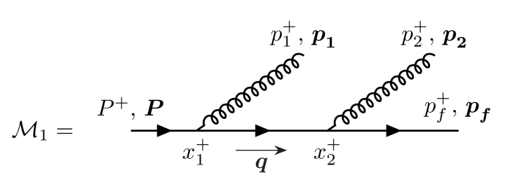
Figure 1: First diagram, $\mathcal{M}_{1}$.

We begin by considering the diagram $\mathcal{M}_{1}$ shown in figure 1, where taking the soft limit for both emissions implies $\alpha_{1},\alpha_{2}\ll\alpha_{f}\sim 1$. In this kind of diagrams, each vertex comes with a phase factor consisting of the four-position of the vertex times the difference between the outgoing and the incoming four-momenta. Upon integration on the minus component of the four-momentum in the intermediate propagator,

$$\int{\rm d}q^{-}\,\frac{e^{i(p_{1}+q-P)\cdot x_{1}+i(p_{2}+p_{f}-q)\cdot x_{2}}}{q^{2}+i\epsilon}=\int{\rm d}q^{-}\,\frac{e^{i(p_{1}+q-P)\cdot x_{1}+i(p_{2}+p_{f}-q)\cdot x_{2}}}{2q^{+}\left[q^{-}-\frac{\bm{q}^{2}}{2q^{+}}+i\epsilon\right]}$$ (1)

$$\propto \Theta\left(x_{2}^{+}-x_{1}^{+}\right)\exp\left[i\left(p_{1}^{-}+\frac{\bm{q}^{2}}{2q^{+}}-P^{-}\right)x_{1}^{+}+i\left(p_{2}^{-}+p_{f}^{-}-\frac{\bm{q}^{2}}{2q^{+}}\right)x_{2}^{+}\right]\,,$$

the + position of the vertices appears in the phase. Specifically, in this diagram, the position of the second splitting $x_{2}^{+}$ appears only in one of the phase factors in (1), with its phase given by the imbalance of the minus component of the momenta at the vertex, computed when all momenta are on-shell, while the forward and transverse momenta components are conserved. This phase factor, is usually denoted as $e^{i\Delta E_{2f}x_{2}^{+}}$, where the so-called energy denominator $\Delta E_{2f}$ is given by

$$\Delta E_{2f} =\big{(}p^{-}_{2}+p^{-}_{f}-q^{-}\big{)}_{\rm on-shell}=\frac{\bm{p}_{2}^{2}}{2p_{2}^{+}}+\frac{\bm{p}_{f}^{2}}{2p_{f}^{+}}-\frac{|\bm{p}_{2}+\bm{p}_{f}|^{2}}{2(p_{2}^{+}+p_{f}^{+})}=\frac{P^{+}}{2}\frac{\alpha_{2}\alpha_{f}}{\alpha_{2}+\alpha_{f}}\left|\bm{\theta}_{2f}\right|^{2},$$ (2)

where we have defined the transverse vector

$$\bm{\theta}_{2f} =\frac{\bm{p}_{2}}{\alpha_{2}P^{+}}-\frac{\bm{p}_{f}}{\alpha_{f}P^{+}}\,.$$ (3)

When the transverse momenta are much smaller than the forward components, the variable $\bm{\theta}_{2f}$ can be interpreted as the opening angle between the final quark and gluon 2. This quantity is also referred to as the relative transverse velocity, $\bm{v}_{2f}$.

The same prescription can be followed for the first vertex with position $x^{+}_{1}$, resulting in the phase-factor $e^{i\Delta E_{q1}x_{1}^{+}}$, where $\Delta E_{q1}$ is given by

$$\Delta E_{q1} =\left(p^{-}_{1}+q^{-}-P^{-}\right)_{\rm on-shell}=\frac{\bm{p}_{1}^{2}}{2\alpha_{1}P^{+}}+\frac{|\bm{p}_{2}+\bm{p}_{f}|^{2}}{2(\alpha_{f}+\alpha_{2})P^{+}}-\frac{|\bm{p}_{1}+\bm{p}_{2}+\bm{p}_{f}|^{2}}{2P^{+}}\,.$$ (4)

These two phase factors are the only necessary quantities to perform the double $x^{+}$ integration in the amplitude, resulting in

$$\mathcal{M}_{1}\propto\int_{0}^{\infty}dx_{1}^{+}\int_{0}^{\infty}dx_{2}^{+}\ e^{i\Delta E_{q1}x_{1}^{+}}e^{i\Delta E_{2f}x_{2}^{+}}\Theta(x_{2}^{+}-x_{1}^{+})\propto\frac{1}{\Delta E_{2f}}\,\frac{1}{\Delta E_{q1}+\Delta E_{2f}}\,,$$ (5)

where the $i\epsilon$ prescription, which regulates the behaviour at infinity, has been left implicit.

This integration is enough to observe that the large logarithmic behaviour arises from the region where $(\Delta E_{q1}+\Delta E_{2f})\to 0$, with $\Delta E_{q1}\gg\Delta E_{2f}$. Defining the respective formation times as the inverse factors in the phases,

$$t_{f1}=\frac{1}{\Delta E_{q1}}\,,\qquad\text{and}\qquad\ t_{f2}=\frac{1}{\Delta E_{2f}}\,,$$ (6)

the logarithmic enhancement originates from the region $t_{f2}\gg t_{f1}$.

To characterise the enhanced regions of phase space as a function of the final momenta, it is useful to express the second denominator in eq. (5) as a function of the final state quantities, yielding the following form:

$$\Delta E_{12f} = \Delta E_{q1}+\Delta E_{2f}$$ (7)

$$= \frac{\bm{p}_{1}^{2}}{2\alpha_{1}P^{+}}+\frac{\bm{p}_{2}^{2}}{2\alpha_{2}P^{+}}+\frac{\bm{p}_{f}^{2}}{2\alpha_{f}P^{+}}-\frac{|\bm{p}_{1}+\bm{p}_{2}+\bm{p}_{f}|^{2}}{2P^{+}}$$

$$= (\alpha_{1}+\alpha_{f})\Delta E_{1f}+(\alpha_{2}+\alpha_{f})\Delta E_{2f}+(\alpha_{1}+\alpha_{2})\Delta E_{12}\,,$$

where $\Delta E_{ij}$ are defined, in analogy with eq. (2), as

$$\Delta E_{ij}=\frac{P^{+}}{2}\frac{\alpha_{i}\alpha_{j}}{\alpha_{i}+\alpha_{j}}|\bm{\theta}_{ij}|^{2}\,,\qquad\text{ with }\qquad\bm{\theta}_{ij}=\frac{\bm{p}_{i}}{\alpha_{i}P^{+}}-\frac{\bm{p}_{j}}{\alpha_{j}P^{+}}\,.$$ (8)

Taking the soft limit $\alpha_{1},\alpha_{2}\ll\alpha_{f}\sim 1$ for each energy factor, one finds:

$$\Delta E_{1f}\simeq\frac{P^{+}}{2}\alpha_{1}\bm{\theta}^{2}_{1f}\,,\quad\Delta E_{2f}\simeq\frac{P^{+}}{2}\alpha_{2}\bm{\theta}^{2}_{2f}\,,\quad\Delta E_{12}=\frac{P^{+}}{2}\frac{\alpha_{1}\alpha_{2}}{\alpha_{1}+\alpha_{2}}\bm{\theta}^{2}_{12}\,,$$ (9)

which implies for the energy denominator in eq. (7)

$$\Delta E_{12f}\sim\Delta E_{1f}+\Delta E_{2f}+(\alpha_{1}+\alpha_{2})\Delta E_{12}\,.$$ (10)

From the definitions of the light cone angles, the following constraint holds:

$$\bm{\theta}_{12}+\bm{\theta}_{2f}+\bm{\theta}_{f1}=\bm{0}\,,$$ (11)

where $\bm{\theta}_{ji}=-\bm{\theta}_{ij}$ is implicitly used. This constraint implies that if one of the angles is much smaller than the others, the remaining two must be similar in magnitude. We therefore identify three phase-space regions of interest:

• Region I: $\bm{\theta}^{2}_{2f}\ll\bm{\theta}^{2}_{1f}\sim\bm{\theta}^{2}_{12}\iff\alpha_{1}\Delta E_{2f}\ll\alpha_{2}\Delta E_{1f}\sim(\alpha_{1}+\alpha_{2})\Delta E_{12}$ ;

• Region II: $\bm{\theta}^{2}_{1f}\ll\bm{\theta}^{2}_{2f}\sim\bm{\theta}^{2}_{12}\iff\alpha_{2}\Delta E_{1f}\ll\alpha_{1}\Delta E_{2f}\sim(\alpha_{1}+\alpha_{2})\Delta E_{12}$ ;

• Region III: $\bm{\theta}^{2}_{12}\ll\bm{\theta}^{2}_{1f}\sim\bm{\theta}^{2}_{2f}\iff(\alpha_{1}+\alpha_{2})\Delta E_{12}\ll\alpha_{1}\Delta E_{2f}\sim\alpha_{2}\Delta E_{1f}$ .

Recalling that the amplitude $\mathcal{M}_{1}$ has a double-logarithmic structure and the formation times are given by

$$\mathcal{M}_{1}\propto\frac{1}{\Delta E_{12f}}\frac{1}{\Delta E_{2f}}\,,\,\,t^{-1}_{f1}=\Delta E_{12f}-\Delta E_{2f}\simeq\Delta E_{1f}+(\alpha_{1}+\alpha_{2})\Delta E_{12}\,,\,\,t^{-1}_{f2}=\Delta E_{2f}\,,$$ (12)

we see that $\mathcal{M}_{1}$ is enhanced — meaning that the smallness of one denominator implies the smallness of the other — in regions I and III. Specifically, the double logarithmic enhancement in region I requires that $\alpha_{2}/\alpha_{1}$ is not much larger than unity. In the case of region III, the enhanced region corresponds to $\alpha_{1}\gg\alpha_{2}$. In both cases, the first formation time becomes $t^{-1}_{f1}\simeq\Delta E_{1f}$, and the enhanced regions can be expressed as $\Delta E_{1f}\gg\Delta E_{2f}$.

Figure 2: Second diagram, $\mathcal{M}_{2}$.

We consider now the amplitude $\mathcal{M}_{2}$, depicted in figure 2. The logarithmically enhanced regions can be obtained from the $\mathcal{M}_{1}$ results by simply swapping the gluon labels $1\leftrightarrow 2$, and interchanging the regions $\textrm{I}\leftrightarrow\textrm{II}$. Consequently, $\mathcal{M}_{2}$ is enhanced in region II provided that $\alpha_{1}/\alpha_{2}$ is not much larger than unity, and in region III given that $\alpha_{2}\gg\alpha_{1}$. The enhanced regions satisfy the condition $\Delta E_{2f}\gg\Delta E_{1f}$, and thus do not overlap with those of amplitude $\mathcal{M}_{1}$.

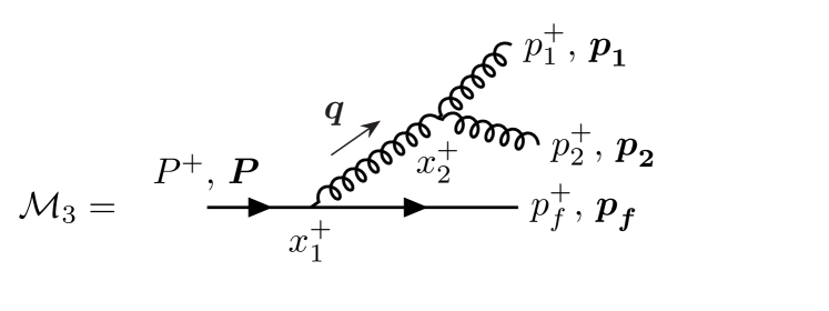
Figure 3: Third diagram, $\mathcal{M}_{3}$.

Next, we turn to amplitude $\mathcal{M}_{3}$, illustrated in figure 3. Its double logarithmic structure and formation times are given by

$$\mathcal{M}_{3}\propto\frac{1}{\Delta E_{12f}}\frac{1}{\Delta E_{12}}\,,\,\,t^{-1}_{f1}=\Delta E_{12f}-\Delta E_{12}\simeq\Delta E_{1f}+\Delta E_{2f}-\Delta E_{12}\,,\,\,t^{-1}_{f2}=\Delta E_{12}\,,$$ (13)

where $\Delta E_{12f}$ is defined in eq. (7) and can also be written as $\Delta E_{12f}=\Delta E_{qf}+\Delta E_{12}$. Additionally, the soft limit implies a strong ordering of gluon energies: either $\alpha_{1}\gg\alpha_{2}$ or $\alpha_{1}\ll\alpha_{2}$. Analysing each of the regions, we see that $\mathcal{M}_{3}$ is logarithmically enhanced in all three. In region I, where $\alpha_{1}\gg\alpha_{2}$, we have $\Delta E_{1f}\gg\Delta E_{2f}\sim\Delta E_{12}$. This implies $\Delta E_{12f}\sim\Delta E_{1f}\sim t^{-1}_{f1}$, and $t^{-1}_{f2}=\Delta E_{12}\sim\Delta E_{2f}$. In region II, the enhancement is analogous but with the gluons’ labels interchanged. Finally, in region III the enhancements occur in both cases: $\alpha_{1}\gg\alpha_{2}$ leading to $\Delta E_{1f}\gg\Delta E_{2f}\gg\Delta E_{12}$, and $\alpha_{2}\gg\alpha_{1}$ leading to $\Delta E_{2f}\gg\Delta E_{1f}\gg\Delta E_{12}$. In both cases, the condition for double logarithmic enhancement can be written as the formation time of the first splitting being much smaller than that of the second one, $t_{f1}\ll t_{f2}$.

The formation times for each of the two splittings in all three regions for all amplitudes are summarised in table 1. We note the logarithmic enhancement of several interference terms, as evidenced by the presence of more than one entry per column. Further, in regions I and II all relevant amplitudes are characterised by analogous formation times (at least in the enhanced regions). However, in region III these enhancements have a slightly different space-time structure: while both $\mathcal{M}_{1}$ and $\mathcal{M}_{3}$ show enhancements for this angular configuration, the formation times of their second splittings ($t_{f2}$) are well separated.

	Region I $\bm{\theta}^{2}_{2f}\ll\bm{\theta}^{2}_{1f}\sim\bm{\theta}^{2}_{12}$	Region II $\bm{\theta}^{2}_{1f}\ll\bm{\theta}^{2}_{2f}\sim\bm{\theta}^{2}_{12}$	Region III $\bm{\theta}^{2}_{12}\ll\bm{\theta}^{2}_{1f}\sim\bm{\theta}^{2}_{2f}$
$\mathcal{M}_{1}$	$t^{-1}_{f1}\sim\Delta E_{1f}$ $t^{-1}_{f2}=\Delta E_{2f}$ $\Delta E_{1f}\gg\Delta E_{12}\gtrsim\Delta E_{2f}$	—–	$t^{-1}_{f1}\sim\Delta E_{1f}$ $t^{-1}_{f2}=\Delta E_{2f}$ $\Delta E_{1f}\gg\Delta E_{2f}\gg\Delta E_{12}$
$\mathcal{M}_{2}$	—–	$t^{-1}_{f1}\sim\Delta E_{2f}$ $t^{-1}_{f2}=\Delta E_{1f}$ $\Delta E_{2f}\gg\Delta E_{12}\gtrsim\Delta E_{1f}$	$t^{-1}_{f1}\sim\Delta E_{2f}$ $t^{-1}_{f2}=\Delta E_{1f}$ $\Delta E_{2f}\gg\Delta E_{1f}\gg\Delta E_{12}$
$\mathcal{M}_{3}$	$t^{-1}_{f1}\sim\Delta E_{1f}$ $t^{-1}_{f2}=\Delta E_{12}$ $\Delta E_{1f}\gg\Delta E_{12}\sim\Delta E_{2f}$	$t^{-1}_{f1}\sim\Delta E_{2f}$ $t^{-1}_{f2}=\Delta E_{12}$ $\Delta E_{2f}\gg\Delta E_{12}\sim\Delta E_{1f}$	$t^{-1}_{f1}\sim\Delta E_{1f}$ $t^{-1}_{f2}=\Delta E_{12}$ $\Delta E_{1f}\gg\Delta E_{2f}\gg\Delta E_{12}$ (*)

Table 1: Formation times, defined as the phase-factors for the $x^{+}$ integrations in the amplitudes, for all three diagrams, in all three regions of interest. In all cases, logarithmic enhancements correspond to $t^{-1}_{f1}\gg t^{-1}_{f2}$. (*) In region III, $\mathcal{M}_{3}$ also admits the labels’ interchange $1\leftrightarrow 2$.

The outcome of this section is that for all three diagrams contributing to the $q\to qgg$ process, formation times for each splitting can be consistently defined in all regions that lead to double logarithms, where they are strongly ordered. It is therefore reasonable to use formation time as an evolution variable that effectively captures the double logarithmic regions in the parton shower.

3 Building differently ordered parton cascades

A parton shower consists of multiple parton emissions generated through a Markovian $1\rightarrow 2$ (or 2$\rightarrow 3$) process, in which the splitting probability is calculable within perturbative QCD. In the leading logarithmic approximation, the splitting rate for a specific parton branching process, $a\rightarrow b+c$, occurring at some resolution scale $s$ where parton $b$ carries an energy fraction $z$ from the parent parton, is given by

$${\rm d}\mathcal{P}_{a\rightarrow bc}=\frac{{\rm d}s}{s}\,\frac{\alpha}{2\pi}\,\hat{P}_{a\rightarrow bc}(z)\,{\rm d}z\,,$$ (14)

where $\alpha$ is the QCD coupling constant and $\hat{P}_{a\rightarrow bc}(z)$ is the Altarelli-Parisi splitting kernel for the branching process under consideration Gribov:1972ri ; Gribov:1972rt ; Altarelli:1977zs ; Dokshitzer:1977sg . At tree-level, the unregularized parton splitting probabilities are given by:

$$\hat{P}_{q\rightarrow gq}(z) =\hat{P}_{q\rightarrow qg}(1-z)=C_{\rm F}\,\frac{1+(1-z)^{2}}{z}\,,$$ (15)

$$\hat{P}_{g\rightarrow gg}(z) =C_{\rm A}\left(\frac{z}{1-z}+\frac{1-z}{z}+z(1-z)\right)\,,$$ (16)

$$\hat{P}_{g\rightarrow q\bar{q}}(z) =T_{\rm F}\left(z^{2}+(1-z)^{2}\right)\,,$$ (17)

where $C_{\rm F}=4/3$, $C_{\rm A}=3$, and $T_{\rm F}=1/2$ correspond to SU(3) invariants.

To generate the splitting scales, $s$, and momentum fractions, $z$, for all splittings in a parton cascade, a parton shower samples the survival probability for each parton species $a$ with respect to a specific $1\rightarrow 2$ process between two scales. At leading logarithmic order, this probability is given by the Sudakov form factor, derived through analytical resummation:

$$\Delta_{a\rightarrow bc}(s_{\rm prev},s_{\rm next})=\exp\left\{-\int^{s_{\rm prev}}_{s_{\rm next}}\frac{{\rm d}s}{s}\,\frac{\alpha(s)}{2\pi}\int_{\Gamma(s)}\hat{P}_{a\rightarrow bc}(z)\,{\rm d}z\right\}\,,$$ (18)

where $s_{\rm prev}$ and $s_{\rm next}$ respectively denote to the scales at which the parton is produced and decays into two new partons. The integration over the splitting scale is performed within the interval $[s_{\rm prev},s_{\rm next}]$, while the energy fraction is integrated over the available phase space $\Gamma(s)$ determined by the splitting scale. The specific functional form of $\Gamma(s)$ depends on the details of the parton shower implementation. To account for running coupling effects, the scale dependence of $\alpha(s)$ is explicitly considered.

In the double leading logarithmic approximation (DLA) only the divergent parts of the splitting kernels $\hat{P}_{a\rightarrow bc}$ are considered, and thus the $g\rightarrow q\bar{q}$ process does not contribute at this level of accuracy. From eqs. (15) and (16), it is straightforward to see that the splitting kernels at DLA accuracy can be expressed as:

$$\hat{P}(z) =\frac{2\,C_{\rm R}}{z}\,,$$ (19)

with $C_{\rm R}$ standing for $C_{\rm F}$ ($C_{\rm A}$) in the case of the emitter being a quark (gluon). The double leading logarithmic form for the survival probability is thus given by

$$\Delta_{\rm R}(s_{\rm prev},s_{\rm next})=\exp\left\{-\,\frac{\alpha\,C_{\rm R}}{\pi}\int^{s_{\rm prev}}_{s_{\rm next}}\frac{{\rm d}s}{s}\int_{\Gamma(s)}\frac{{\rm d}z}{z}\right\}\,,$$ (20)

where the coupling strength $\alpha$ has been taken as a constant for simplicity.

As previously mentioned, addressing these divergences requires a regularisation procedure tailored to the specific details of the parton shower algorithm. This involves defining the selection criteria for $\Gamma(s)$, which is closely linked to the choice of the ordering variable. The primary objective of this manuscript is to examine the potential impacts of varying the ordering variables within a parton shower framework, regardless the specific implementation details. To achieve this, we define $\Gamma(s)$ by introducing a threshold scale $s_{\rm min}$ beyond which additional radiation is no longer emitted. This approach ensures consistency in the definition of the phase space across all choices of $s$.

3.1 Ordering variables and the momentum scheme

To define the splitting scales $s$, we use light-cone coordinates, where four-momenta $p^{\mu}=(p^{+},p^{-},\bm{p})$, are written as

$$p^{\pm}=\frac{p^{0}\pm p^{3}}{\sqrt{2}}\,,\,\bm{p}=(p^{1},p^{2})\,.$$ (21)

Requiring full energy-momentum conservation in a generic splitting $p_{a}\to p_{b}+p_{c}$ leads to

$$z =p^{+}_{b}/p^{+}_{a}=1-p^{+}_{c}/p^{+}_{a}\,,$$ (22)

$$\bm{p}_{a} =\bm{p}_{b}+\bm{p}_{c}\,,$$ (23)

$$|\bm{\kappa}|^{2} =z(1-z)\,p^{2}_{a}-(1-z)\,p^{2}_{b}-z\,p^{2}_{c}\,,$$ (24)

$z$ is the forward (+) momentum fraction of parton $b$, $p^{2}_{i}$ corresponds to the invariant mass of parton $i$, and $\bm{\kappa}\equiv(1-z)\,\bm{p}_{b}-z\,\bm{p}_{c}$ is the relative transverse momentum between the daughter partons $b$ and $c$. Based on (24), we define three different ordering variables: the inverse formation time $\tau^{-1}$ (see section 2), the invariant mass $m^{2}$, and the (squared) opening angle $\theta^{2}$, given respectively by

$$\tau^{-1} =\frac{|\bm{\kappa}|^{2}}{E\,z(1-z)}\,,$$ (25a)

$$m^{2} =\frac{|\bm{\kappa}|^{2}}{z(1-z)}\,,$$ (25b)

$$\theta^{2} =\frac{|\bm{\kappa}|^{2}}{[E\,z(1-z)]^{2}}\,,$$ (25c)

where $E=p^{+}/\sqrt{2}$ serves as a proxy for the energy of the incoming parton.

In these definitions, we have implicitly chosen to connect the splitting scales $s$ to the relative transverse momentum $\bm{\kappa}$ , such that for all ordering choices, $|\bm{\kappa}|=\kappa(s,z)$. We refer to this component of the parton shower implementation as the kinematic scheme, and to this specific instance as the “momentum scheme” or “$|\bm{\kappa}|^{2}$ scheme”. One advantage of this choice is that it simplifies the requirement for all perturbative splittings to have transverse momentum above some cutoff given by the hadronisation scale. In this scheme, this condition is directly implemented through the integration bounds in the exponent of the survival probability in eq. (20). On the other hand, the invariant mass of the particles does not correspond to any particular splitting scale, with the $m^{2}$ variable serving only as a lower bound on $p^{2}_{a}$.

3.1.1 Starting and stopping conditions

Now that the ordering variables have been defined, we turn our attention to the next essential ingredient for generating QCD radiation via parton showers: the starting and stopping conditions. These conditions initialise the generation of radiation through an upper bound in eq. (20) for the first emission and set a minimum scale that defines the threshold at which the generation of radiation stops. In the broader context of event generators, these scales are determined by the hard scattering matrix element and the hadronisation condition, respectively. In this manuscript, to ensure consistency across the different ordering variables defined in eq. (25), we fix the stopping condition as $|\bm{\kappa}|=\Lambda$, allowing the shower to continue while $|\bm{\kappa}|^{2}\geq\Lambda^{2}$. For instance, using $\tau^{-1}$ ordering, the stopping criterion yields

$$z(1-z)\geq\frac{\Lambda^{2}/E}{\tau^{-1}}\,.$$ (26)

Since $z(1-z)\leq 1/4$ by construction, eq. (26) also implies a minimum value for the ordering variable,

$$\tau^{-1} \geq\frac{4\Lambda^{2}}{E}\,.$$ (27)

This procedure allows us to define a minimum scale for all ordering variables, denoted as $s_{\rm min}$. For each of the ordering variable, $\tau^{-1}$, $m$ and $\theta$, the scale $s_{\rm min}$ can be interpreted respectively as the (inverse) hadronisation time scale, the hadronisation mass, and the minimum opening angle, for a splitting with mass $\sim\Lambda$ and energy $E$. The corresponding expressions are provided in table 2.

$s$	$s_{\rm min}$	$s_{\rm max}$	$b$
$\tau^{-1}$	$4\Lambda^{2}/E$	$E$	1
$m^{2}$	$4\Lambda^{2}$	$E^{2}$	1
$\theta^{2}$	$16\Lambda^{2}/E^{2}$	$4$	$1/2$

Table 2: Starting ($s_{\rm max}$) and stopping ($s_{\rm min}$) scales of the cascade generated using the three ordering prescriptions $s$. For details on the soft regulator parameter $b$, we refer to subsection 3.1.2.

Turning to the starting condition $s_{\rm max}$, a natural choice is to require the formation time of the first splitting to be larger than the time scale of the hard scattering, which is set by the energy of the first parton, $\tau^{-1}\leq E$. This condition also implies that $m^{2}\leq E^{2}$. However, for $\theta^{2}$, we find:

$$\frac{1}{z(1-z)}\geq\theta^{2}\,,$$ (28)

which presents a problem, as it introduces an additional dependence on the energy fraction $z$ when ordering in $\theta^{2}$. To resolve his issue, we impose the following additional condition on the angular proxy: $\theta^{2}_{\rm max}\geq\theta^{2}$, where $\theta^{2}_{\rm max}$ can be fixed by ensuring consistency with the condition on the formation time (or, alternatively by ensuring the invariant mass is lower than the parton energy),

$$\tau^{-1}=E\,z(1-z)\,\theta^{2}\Longrightarrow\tau^{-1}\leq E\,\frac{1}{4}\,\theta^{2}_{\rm max}\,.$$ (29)

This implies a maximum value for the angular proxy $\theta^{2}\leq 4$. These conditions, when rewritten for an arbitrary ordering scale $s$, provide the maximum and minimum allowed values, $s_{\rm max}$ and $s_{\rm min}$ respectively, listed in table 2.

3.1.2 The parton shower algorithm

With the starting and stopping conditions consistently defined for all ordering variables, it is possible to generate the parton shower by sampling of the survival probability (20). The principal challenge lies in the integration region for the energy fraction $z$ of resolvable splittings, denoted as $\Gamma(s)$. Specifically, (26) sets the minimum value for the energy fraction, $z_{\rm min}$, and fully determines the available phase space for perturbative emissions to be $z\in[z_{\rm min},1-z_{\rm min}]$, with

$$z_{\rm min}=\frac{1}{2}-\frac{1}{2}\sqrt{1-\left(\frac{s_{\rm min}}{s}\right)^{b}}\,,$$ (30)

where $b$ = 1 for $\tau^{-1}$, and $m^{2}$ and $b$ = 1/2 for $\theta^{2}$ (see table 2).

Although this leads to a potentially complicated integral in (20) with no closed analytic form, this complexity can be managed using a veto algorithm Bierlich:2022pfr ; Lonnblad:2012hz . In this approach, the survival probability is computed in an extended phase space $\bar{\Gamma}(s)$. Any emissions sampled outside the true phase space $\Gamma(s)$ are discarded, and the scale of the discarded emission becomes a new (lower) scale for subsequent radiation. This process continues until a resolvable splitting is found or the scale falls below $s_{\rm min}$.

The extended phase space can be identified by noting that

$$z_{\rm min} >\frac{1}{4}\left(\frac{s_{\rm min}}{s}\right)^{b}\equiv z_{\rm cut}(s)\,.$$ (31)

Under this parameterisation, the survival probability (20) becomes

$$\Delta_{\rm R}(s_{\rm prev},s_{\rm next}) =\exp\left\{-\frac{\alpha C_{\rm R}}{\pi}\int^{s_{\rm prev}}_{s_{\rm next}}\frac{{\rm d}s}{s}\int^{1}_{z_{\rm cut}(s)}\frac{{\rm d}z}{z}\right\}$$ (32)

$$=\exp\left\{-\frac{\alpha C_{\rm R}}{\pi}\,\frac{b}{2}\,\left[\ln^{2}\left(\frac{4^{1/b}s_{\rm prev}}{s_{\rm min}}\right)-\ln^{2}\left(\frac{4^{1/b}s_{\rm next}}{s_{\rm min}}\right)\right]\right\}\,,$$ (33)

highlighting the large logarithmic enhancements in QCD radiation.

With these definitions, the parton shower algorithm proceeds as follows for a given $E$ and $\Lambda$:

1. Sample a splitting scale $s_{\rm trial}$ from the survival probability in eq. (33), with the previous scale $s_{\rm prev}$ given by either the previous splitting or the maximum kinematically allowed value $s_{\rm max}$. This amounts to solving the equation

   $$\Delta_{\rm R}(s_{\rm prev},s_{\rm trial})=\mathcal{R}_{s}\,,$$ (34)

   where $\mathcal{R}_{s}$ is a random number uniformly sampled in the interval $[0,1]$.

2. Sample an energy fraction $z_{\rm trial}$ according to the DLA splitting kernel in (19), considering the interval $[z_{\rm cut}(s_{\rm trial}),1]$. In this case, one must solve

   $$\frac{\ln(z_{\rm trial}/z_{\rm cut})}{\ln(1/z_{\rm cut})}=\mathcal{R}_{z}\,,$$ (35)

   where $\mathcal{R}_{z}$ is another random number uniformly sampled in the interval $[0,1]$.

3. Compute the relative transverse momentum $|\bm{\kappa}|_{\rm trial}$ and the angular proxy $\theta_{\rm trial}$ associated with the sampled pair $(s_{\rm trial},z_{\rm trial})$ using eq. (25). If the conditions

   $$|\bm{\kappa}|_{\rm trial}\geq\Lambda\,,\qquad\textrm{and}\,\qquad\theta_{\rm trial}^{2}\leq 4\,\,,$$ (36)

   are satisfied, the trial emission is accepted and $(s_{\rm trial},z_{\rm trial})$ is recorded as part of the cascade. Add two new partons with energies $zE$ and $(1-z)E$, respectively, and continue the process iteratively for each outgoing particle. If the conditions (36) are mot met, reject the trial emission and repeat step 1) with the updated maximum scale $s_{\rm prev}=s_{\rm trial}$.

4. When the maximum allowed splitting scale is below $s_{\rm min}$, terminate the present branch of the shower and flag the last parton as a “final state” particle.

This approach ensures consistent application of the soft regulator, as well as the starting and stopping conditions across different ordering variables. Consequently, any visible differences between parton showers are attributable to the choice of the ordering parameter. It should be noted that this algorithm provides the relative transverse momentum $\bm{\kappa}$ and the forward momentum $p^{+}$, while the $p^{-}$ components remains unspecified. These can be obtained by selecting a different kinematic scheme or by imposing an on-shell condition on the final partons at each stage of the shower, shifting momentum to a “recoiler” (see Campbell:2022qmc ). Given that all these choices modify the parton shower output of the parton shower, this work focuses on the splitting scales $s$ and energy fractions $z$ sampled from the survival probability and splitting kernels, respectively.

3.2 The mass scheme

It is important to highlight that the choice of defining the ordering variables in terms of the relative transverse momentum $|\bm{\kappa}|^{2}$ is not unique. Alternatively, they can be expressed in terms of the invariant mass of the mother particle $p_{a}^{2}$, with the relative transverse momentum computed using eq. (24). In this approach, the ordering variables are given by

$$\tau^{-1}_{*}=\frac{p_{a}^{2}}{E}\,,\qquad m_{*}^{2}=p_{a}^{2}\,,\qquad\theta_{*}^{2}=\frac{p_{a}^{2}}{E^{2}\,z(1-z)}\,.$$ (37)

Accordingly, we also define a proxy for the relative transverse momentum, based on (24),

$$|\bm{\kappa}_{*}|^{2}=z(1-z)\,p^{2}_{a}\,.$$ (38)

Expressing all ordering variables as functions of the invariant mass of the parent parton leads to a kinematic scheme where the four-momenta of a splitting $p_{a}\to p_{b}+p_{c}$ are chosen such that $p^{2}_{a}=m_{*}^{2}$. Hence, we call this scheme the “$p^{2}$ scheme” or “mass scheme”. We note that this choice will, in general, produce kinematic distributions different from those of the “momentum scheme” described in the section 3.1.

This scheme requires some modifications to the parton shower algorithm, namely to the resolution conditions in eqs. (36). Since the angular proxy $\theta^{2}$ and the relative transverse momentum $|\bm{\kappa}|$ are not available when the splitting is generated, these conditions must be imposed on the proxy variables, $\theta_{*}$ and $|\bm{\kappa}_{*}|$. Thus, the resolution conditions for the mass scheme are

$$4\geq\theta_{*}^{2}\geq\theta^{2}\,,$$ (39a)

$$|\bm{\kappa}_{*}|^{2}\geq|\bm{\kappa}|^{2}\geq\Lambda^{2}\,,$$ (39b)

where we have highlighted the fact that $\theta_{*}$, and $|\bm{\kappa}_{*}|$ serve as upper bounds for their “momentum scheme” counterparts and coincide with these counterparts when the daughter partons are massless.

From eqs. (39) we note that while the condition $4\geq\theta_{*}^{2}$ implies its “momentum scheme” analogue $4\geq\theta^{2}$, the condition $|\bm{\kappa}_{*}|^{2}\geq\Lambda^{2}$ does not imply $|\bm{\kappa}|^{2}\geq\Lambda^{2}$ . To enforce this resolution condition, we recognise that the relative transverse momentum of a splitting $a\to b+c$ constrains the invariant masses of the daughter partons $b$ and $c$ in a non-trivial way, as described by

$$|\bm{\kappa}|^{2}=z(1-z)p^{2}_{a}-(1-z)p^{2}_{b}-zp^{2}_{c}\geq\Lambda^{2}\,.$$ (40)

This implies that the evolution of any parton is constrained by that of its sibling. To address this, we evolve the pair of particles in parallel. Initially, the invariant masses of $b$ and $c$ are subject to overly permissive constraints when generating their trial scales:

$$z\,p^{2}_{a} >p^{2}_{b}\,,$$ (41a)

$$(1-z)\,p^{2}_{a} >p^{2}_{c}\,.$$ (41b)

If any pair disobeys the actual constraint in eqs. (41), both splittings are retried according to the veto procedure described above. Although alternative methods exist Webber:1986mc , such as randomly selecting which daughter to sample first or always choosing the more energetic parton first, these differences are expected to be subdominant in the double logarithmic approximation.

We further note how the condition on the relative transverse momentum (40) can be expressed in terms of formation times,

$$|\bm{\kappa}|^{2}=Ez(1-z)\left(\tau^{-1}_{*\,a}-\tau^{-1}_{*\,b}-\tau^{-1}_{*\,c}\right)\geq\Lambda^{2}\,,$$ (42)

which implies, analogously to eqs. (41), the following constraints on the formation times:

$$\tau^{-1}_{*\,a} >\tau^{-1}_{*\,b}\,,$$ (43a)

$$\tau^{-1}_{*\,a} >\tau^{-1}_{*\,c}\,,$$ (43b)

ensuring a strictly decreasing formation time throughout the shower.

The differences between these kinematic schemes are twofold. First, the different mappings between the ordering variables and the parton momenta lead to distinct distributions for the kinematic variables such as $\bm{\kappa}$ and $\theta$. This issue can be avoided by using variables related to the evolution scales like $\bm{\kappa}_{*}$ and $\theta_{*}$. Second, and more importantly, the introduction of an additional veto modifies the phase space available for splittings, thereby affecting the structure of the partonic cascade.

In summary, the setup described in this section allows for the construction of a vacuum parton shower framework at double logarithmic accuracy, ensuring consistency across the three different ordering variables specified in (25). The generation of subsequent radiation for each of these definitions is governed by the survival probability (33), with the lower and upper bounds of the ordering variable, as well as the $b$ parameter presented in table 2. For each splitting, given a scale $s$ and energy fraction $z$, the relative transverse momentum of the outgoing particles is determined by applying either the momentum scheme (section 3.1) or the mass scheme (section 3.2).

4 Effect of the ordering variable and kinematic scheme on the parton shower evolution

In this section, we first compare the outcomes of the aforementioned parton showers for the three different ordering variables within the momentum scheme (see section 4.1). In section 4.2, we fix the ordering variable to $\tau^{-1}$ and adopt the kinematic scheme to compute the relative transverse momenta. These comparisons allow us to understand how variations in ordering variables and kinematic schemes influence the output of vacuum parton showers. While, in vacuum, such differences reflect theoretical uncertainties inherent in parton shower approaches rather than physical effects and can generally be mitigated by hadronisation effects, they can become important for jet quenching studies. For such studies, where the resulting space-time picture of each parton shower needs to be integrated with a QGP-like medium, the choice of the ordering variable can impact the effective energy loss induced, as we will demonstrate in section 5.

4.1 Comparison between different ordering variables

The results depicted in this section were obtained by generating $10^{6}$ partonic cascades within the momentum scheme following the three orderings: inverse formation time $\tau^{-1}$, invariant mass $m^{2}$, and squared opening angle $\theta^{2}$. In each case, the parton shower was initialised as a single quark with forward momentum $p^{+}_{\rm jet}/\sqrt{2}=E_{\rm jet}=$1000\text{\,}\mathrm{G}\mathrm{e}\mathrm{V}$$, and was allowed to radiate until the relative transverse momentum of the splittings reach the hadronisation scale $\Lambda=$1\text{\,}\mathrm{G}\mathrm{e}\mathrm{V}\mathrm{/}\mathrm{c}$$. For simplicity, we focus on the quark branch of the parton shower, as it provides the minimal setup to compare the effects of the different ordering variables.

The left panel of figure 4 shows the distribution of the number of splittings along the quark branch, quantifying the average activity along the shower. We note that this distribution is normalised to the total number of generated events. Notably, the number of splittings is larger for showers ordered according to the invariant mass of the splitting particle. This can be understood as a consequence of the different scaling of the stopping condition $s_{\rm min}$ with the energy $E$. For the squared opening angle, inverse formation time, and invariant mass of the emitter, $s_{\rm min}$ scales as $E^{-2}$, $E^{-1}$, and $E^{0}$, respectively. As the energy of the emitter decreases, this threshold $s_{\rm min}$ increases, thereby reducing the available phase space for subsequent emissions.

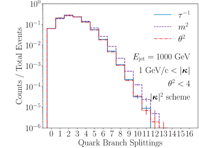
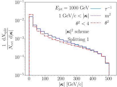
Figure 4: Kinematic distributions for parton cascades generated according to the transverse momentum scheme, for three different ordering prescriptions: $\tau^{-1}$ (blue solid line), $m^{2}$ (purple dashed line), and $\theta^{2}$ (red dash-dotted line). Left: Distribution of the number of quark-initiated splittings. Right: Relative transverse momentum distributions. Histograms are normalised such that their area is unity (left) or to the fraction of events with at least one splitting (right).

In the right panel of figure 4, we present the distribution for the relative transverse momentum of the first splitting $|\bm{\kappa}|$ normalised to the number of events in which at least one emission was generated. We note that since the number of events without emissions is roughly the same across the three ordering variables (see first bin in the left panel of figure 4), normalising against the total number of generated events would yield the same results. Here, the $\tau^{-1}$ and $m^{2}$ ordered showers agree, while they slightly deviate from the $\theta^{2}$-ordered showers. Since $\bm{\kappa}$ is obtained from the ordering variable $s$ and the energy fraction $z$, both sampled from the Sudakov form factor, it generally depends on an interplay between these quantities. However, for the first splitting, it is mainly affected by the different $z$-weights in the variable definitions, with angular ordered showers (which scale with the inverse square of $z(1-z)$) exhibiting a stronger suppression of the high-$\bm{\kappa}$ tail. The mild differences observed in the $\bm{\kappa}$ distribution of the first splitting and the number of splittings along the quark branch clearly indicate that the initialisation conditions were consistently chosen across the different ordering variables.

A more comprehensive description of parton shower structure can be achieved through the Lund plane Dreyer:2018nbf , a two-dimensional representation of the kinematics of perturbative splittings. In this manuscript, we use the angular proxy $\theta$ and the relative transverse momentum $\bm{\kappa}$ as the representative axes for this plane (see appendix A for more details). The resulting jet Lund planes for the first three quark-initiated splittings are shown from left to right in figure 5. The top panel corresponds to the available phase space for $q\to qg$ splittings in time-ordered showers. The middle and bottom panels show the ratios of the equivalent planes for the $m^{2}$ and $\theta^{2}$ ordering variables relative to the $\tau^{-1}$ ordering variable. In the top panel, the Lund plane densities are defined with respect to the total number of events, with the integral of each panel corresponding to the fraction of events with at least 1, 2, or 3 splittings, a normalisation which decreases as the cascade advances. Similarly, in the middle and bottom panels, both the numerator and denominator histograms were computed in this way, making the normalisation of the ratio not straightforward. However, these numerical effects are minor and do not obscure the qualitative interpretation of the results. For a closer examination of how the one dimensional kinematic distributions change with shower development, as well as a quantitative comparison of the spectra obtained with different ordering prescriptions, see appendix B.

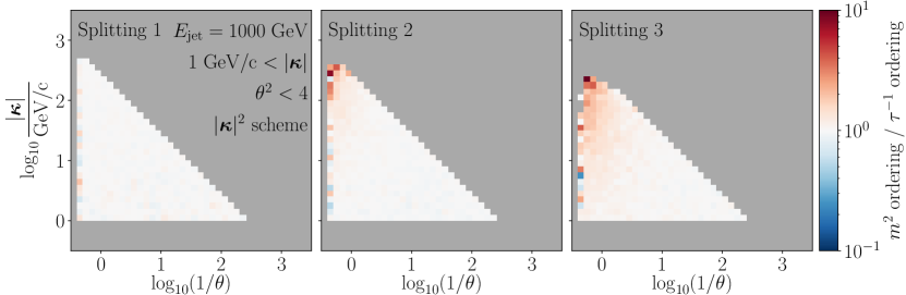
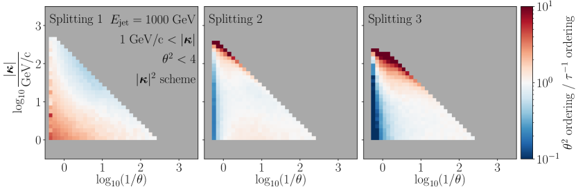
Figure 5: Lund plane distributions in the $(\theta,\bm{\kappa})$ configuration for the first three $q\to qg$ splittings of cascades generated according to the ‘$|\bm{\kappa}|^{2}$ scheme’. Top: Densities for $\tau^{-1}$ ordered cascades. Bins below the minimum are shown in white and empty bins shown in grey. All densities are normalised against the total number of events. Middle: Ratio between $m^{2}$ and $\tau^{-1}$ ordered cascades. Bottom: Ratio between $\theta^{2}$ and $\tau^{-1}$ ordered cascades.

The allowed region corresponds to a right triangle delimited by the boundary conditions defined in eq. (36), which imply

$$\log_{10}(1/\theta)\geq\log_{10}(1/2)\,,\qquad\log_{10}\frac{|\bm{\kappa}|}{$\text{\,}\mathrm{G}\mathrm{e}\mathrm{V}\mathrm{/}\mathrm{c}$}\geq\log_{10}\frac{\Lambda}{$\text{\,}\mathrm{G}\mathrm{e}\mathrm{V}\mathrm{/}\mathrm{c}$}\ ,$$ (44)

with the latter condition reducing to $\log_{10}|\bm{\kappa}|>0$ for the present shower parameters. The upper diagonal limit comes from the bound on the energy fraction $z(1-z)\leq 1/4$, which translates into the following expression:

$$\log_{10}|\bm{\kappa}|\leq-\log_{10}(1/\theta)+\log_{10}\frac{E}{4}\,,$$ (45)

where the limit increases with the jet energy $E_{\rm jet}$. As such, emissions near this threshold can be classified as the “hardest”, while those near the origin as the “softest”.

Having examined the Lund plane distributions, we can use them to further analyse the evolution of partonic showers. For the quark branch ordered by $\tau^{-1}$ (top three panels of figure 5), we observe a migration to smaller values of $\theta$ and $\bm{\kappa}$. This latter trend is mainly driven by the decreasing scale, as $z$ tends to grow with each emission. In the middle panel, the Lund densities for the $m^{2}$-ordered cascades largely coincide with those for $\tau^{-1}$ ordering for the first splitting, though we observe a slight increase in high $\bm{\kappa}$ and wide-angle emissions for subsequent splittings. The lack of a corresponding depletion is due to the differing number of events with at least three splittings, as shown in the left panel of figure 4. Finally, for angular-ordered showers (bottom panels), the first splitting shows an enhancement in the soft (low $z$) region, with a corresponding depletion in hard splittings. In contrast, this behaviour inverts for subsequent splittings, where harder emissions are relatively enhanced. This can be understood as a consequence of the scale dependence of the soft regulator in angular ordering: this causes the splitting function to be more sharply peaked for the first splitting and to flatten faster for subsequent emissions. Since the different ordering prescriptions must converge in the low $|\bm{\kappa}|$ and low $\theta$ corner of the Lund plane, these effects manifest in the high-$\theta$ region.

Overall, the differences arising from varying the ordering prescription are limited to wide-angle emissions. When focusing on the region with angles $\theta\lesssim 0.1$, the Lund density ratios are all compatible with unity. Despite this, when the analysis is restricted to events entirely within the collinear region, the differences between algorithms persist. For more details, see appendix E (discussion near figure 24).

It is also noteworthy that the magnitude of variations due to the changes in the ordering variable, in the range of $\left[10^{-1},10^{1}\right]$, differs from that due to variations in the the kinematic scheme, which range from $0.5$ to $2$. This will be further discussed in section 4.2 (see also figure 9).

To further illustrate the differences between ordering variables, we calculate the Lund plane trajectories. These trajectories are obtained by computing the mean values of the $\theta^{2}$ and $\bm{\kappa}$ distributions from the first five $q\to qg$ splittings in all three algorithms. The trajectories are depicted in figure 6. As previously noted, the $m^{2}$ ordered cascade follows a similar path to the $\tau^{-1}$ ordered shower, taking slightly smaller steps with each splitting due to the different rates at which the phase space is reduced. On the other hand, the $\theta^{2}$-ordered showers follow a markedly different path, taking roughly constant steps in $\log_{10}(1/\theta)$, as it is the ordering variable itself, and in $\log_{10}|\bm{\kappa}|$, since $|\bm{\kappa}|$ is inversely proportional to $\theta$, with $|\bm{\kappa}|/\theta\leq E_{\rm jet}/4$.

In general, all three trajectories start from the same initial point by construction. However, they diverge as the shower develops, with the differences between paths increasing over the emissions. These variations between trajectories quantify the uncertainties inherent to the double logarithmic approximation.

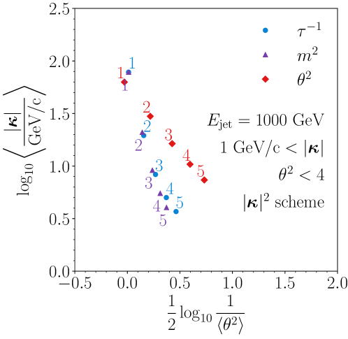
Figure 6: Trajectories in the Lund plane for $\tau^{-1}$ (blue circles), $m^{2}$ (purple triangles), and $\theta^{2}$ (red diamonds) ordered cascades in the $|\bm{\kappa}|^{2}$ kinematic scheme. The values were computed for the first five quark-initiated splittings, and are labelled in the corresponding colours.

4.2 Impact of the kinematic scheme

After analysing the influence of the ordering variable for a given kinematic scheme, we now turn to study the role of the kinematic reconstruction for a given ordering variable, namely the formation time $\tau^{-1}$. This choice of ordering variable is motivated by our final objective of interfacing the parton shower with an evolving medium, as $\tau^{-1}$ can be related to both spatial positions and temporal evolution, making it the most suitable variable for such a setup.

As previously discussed, the kinematic scheme is an integral component of a parton shower’s definition. Typically, comparing different kinematic schemes is considered part of evaluating the accuracy of a the parton shower, and discrepancies between schemes do not directly affect physical outcomes, as they can be adjusted using other parton shower parameters, including those related to non-perturbative physics. However, for our purpose of comparing the effects of different ordering variables on jet quenching, it is essential to assess whether the differences arising from distinct kinematic schemes are comparable in magnitude to those induced by energy loss effects. We do not attempt to provide an exhaustive comparison of all possibilities; instead, we refer to the schemes outlined in section 3 as a guide.

Considering the definitions on section 3, we generated $10^{6}$ events ordered in formation time with both the “momentum scheme” and the “mass scheme”. The showers were initialised as in the previous section: the original parton is a quark with light cone momentum $p^{+}_{\rm jet}/\sqrt{2}=E_{\rm jet}=$1000\text{\,}\mathrm{G}\mathrm{e}\mathrm{V}$$ and the hadronisation scale was set at ${\Lambda=$1\text{\,}\mathrm{G}\mathrm{e}\mathrm{V}\mathrm{/}\mathrm{c}$}$. Once again, we focus on the emissions along the quark branch when comparing these two schemes.

Figure 7 (left) shows the distribution of the number of $q\to qg$ splittings for both kinematic schemes, revealing a more extended distribution for the $|\bm{\kappa}|^{2}$ scheme. This quantifies the differences in the available phase-space region for parton splittings in both schemes. The additional veto imposed in the $p^{2}$ scheme — the retrial procedure imposed on the invariant masses of a quark and its gluon sibling to ensure that their splitting satisfies $|\bm{\kappa}|>\Lambda$ — favours low transverse momentum splittings, reducing the total number of perturbative splittings before the hadronisation scale is reached. A similar effect is observed in the right panel of figure 7, which depicts the relative transverse momentum distributions for both schemes, showing an enhancement of low transverse momentum splittings in the $p^{2}$ scheme. This is another consequence of the faster depletion of phase space for perturbative emissions due to the additional veto.

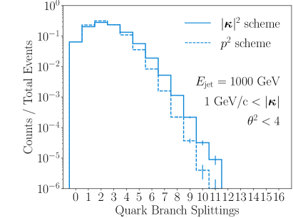
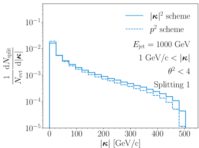
Figure 7: Distributions of the number $q\to qg$ splittings along the quark branch of the parton cascades (left) and the relative transverse momentum of the first quark-initiated splitting (right), for showers generated according to the “momentum scheme” (solid line) and the “mass scheme” (dashed line). The cascades are ordered in formation time, and the distributions are normalised to the total number of events.

To quantify how the shower structure is influenced by the choice of kinematic schemes, we evaluate the extent to which cascades adhere to the angular ordering prescription for coherent soft radiation (Ellis:1996mzs, , Chapter 4). We iterate over the splittings in the quark branch, recording the first splitting whose angular proxy variable $\theta$ is larger than that of its immediate predecessor. The distribution of this “first $\theta^{2}$-inversion location” is shown in figure 8, highlighting that approximately $\sim 20\%$ of all events exhibit at least one inversion, predominantly occurring at the beginning of the cascade, where the phase space for emissions is larger. Accordingly, the $p^{2}$ scheme has a slightly lower probability for angular inversions, a consequence of its relatively restricted phase space.

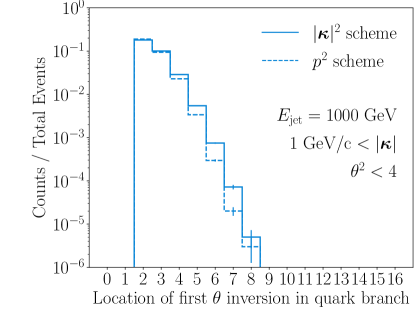
Figure 8: Location of the first angular inversion along the quark branch of parton cascades generated according to the “momentum scheme” (solid line), and the “mass scheme” (dashed line). The cascades are ordered in formation time, and the distributions are normalised to the total number of events.

We now examine how changes in kinematic schemes affect Lund plane distributions. To better evaluate the shower evolution, we focus on two sets of variables introduced in section 3. For the “momentum scheme”, we will continue to use the angular proxy and relative transverse momentum $(\theta,\bm{\kappa})$. In contrast, for the “mass scheme”, we will consider the counterparts to these variables $(\theta_{*},\bm{\kappa}_{*})$, which are more directly connected to the splitting scales and fractions. The relationships between the Lund plane configurations for each set of variables are detailed in appendix A.

With these definitions in mind, figure 9 presents the evolution of cascades generated according to the $p^{2}$ scheme, as a splitting-by-splitting ratio to the $|\bm{\kappa}|^{2}$ scheme over a Lund plane defined in two sets of variables. The top panel depicts the ratio between Lund plane densities evaluated on the variables most natural for each scheme, i.e., the Lund distribution of cascades generated according to the “momentum scheme” in $(\theta,\bm{\kappa})$ variables, divided by the distribution of cascades in the “mass scheme” given in $(\theta_{*},\bm{\kappa}_{*})$ variables, each evaluated at the same point in the respective phase-space. This is indicated by the labels $(\theta_{\rm scheme},\bm{\kappa}_{\rm scheme})$. In this configuration, the ratio between the distributions is close to unity across much of the phase space. Notably, for the first splitting, the ratio is exactly unity because the schemes coincide exactly at this stage. This is due to the fact that the difference between the schemes arises from the constrained evolution of parton pairs sharing the same parent; since the initiating quark does not have a partner, its evolution is unconstrained. As the cascade develops, slight differences between the schemes accumulate, since the veto procedure ensuring $|\bm{\kappa}|\geq\Lambda$ corresponds to enforcing that for some splitting $a\to b+c$ the quantity $\tau^{-1}_{*\,a}-\tau^{-1}_{*\,b}-\tau^{-1}_{*\,c}$ must be strictly positive, a condition slightly stricter than merely time-ordering parton splittings. Accordingly, the second and third splittings present a slight depletion (enhancement) at smaller (larger) values of formation time.

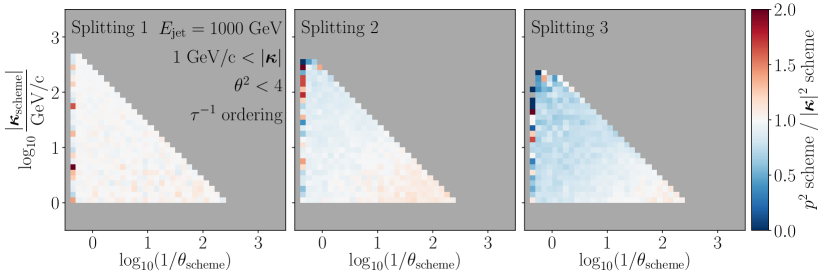
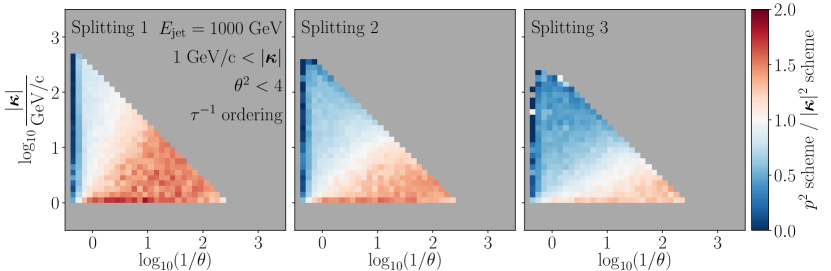
Figure 9: Ratios between Lund plane distributions in both kinematic schemes, for time-ordered cascades. Bins where the denominator vanishes are shown in grey. The ratio is computed between densities using the variables corresponding to each scheme in the top panel. In the bottom pane, the ratio is calculated over the $(\bm{\kappa},\theta)$ pairs.

The bottom panel of figure 9 shows the same ratio in terms of the kinematic variables $|\bm{\kappa}|$ and $\theta$. This Lund plane configuration emphasises the $p^{2}$ scheme’s tendency to favour soft (low $\bm{\kappa}$) and collinear (low $\theta$) splittings, although mapping this region to that of higher values of $\tau$ is less straightforward. It also indicates that the main differences between schemes arise from the definition of kinematic variables rather than the veto imposed during shower generation, at least for time-ordered cascades. This observation is also applicable to mass-ordered cascades, although the impact of different variable definitions is less pronounced in the angular-ordered case, as detailed in appendix C.

Finally, to better quantify the shower evolution, we define trajectories in the Lund plane by computing the average quantities $\langle\theta^{2}\rangle$ and $\langle|\bm{\kappa}|\rangle$, which are the means of the kinematic distributions for the first five quark-initiated splittings of the cascades. These quantities are plotted on a logarithmic scale in figure 10, clearly showing the tendency towards narrower and softer splittings as the cascade approaches the hadronisation scale. The different schemes show similar trajectories, although the “$p^{2}$ scheme” exhibits a larger step size per emission, quantifying the remaining phase space for the evolution of the quark branch. Moreover, a comparable behaviour is observed when ordering parton cascades in terms of the invariant mas $p^{2}$ and angular proxy. This is true in terms of variance across ordering variables and when comparing kinematic schemes with a fixed ordering prescription (compare appendix C to the current and previous sections).

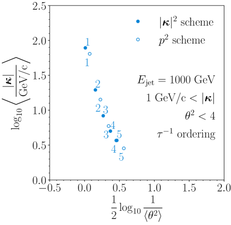
Figure 10: Trajectories in the Lund plane for time-ordered cascades in the $|\bm{\kappa}|^{2}$ scheme (filled circles) and the $p^{2}$ scheme (empty circles), as defined by the mean values of the angular variable $\langle\theta^{2}\rangle$ and relative transverse momentum $\langle|\bm{\kappa}|\rangle$ computed for the first five quark-initiated splittings, and plotted in a logarithmic scale.

4.3 The role of time inversions

Following the same line as in the previous section, we now consider inversions of the formation time $\tau$ and angular variable $\theta^{2}$ along the quark branch of differently ordered cascades. Figure 11 shows the frequency of the first of these inversions along the quark branch, with the left panel depicting $\tau$ inversions, and the right panel showing the analogous distribution for $\theta$ inversions. Notably, time inversions are more likely to occur at the beginning of the cascade, when the phase space is still largely open. Angular-ordered cascades exhibit a larger number of events with at least one formation time inversion ($\sim 29.1\%$ of events) compared to their mass-ordered counterparts ($\sim 11.3\%$ of events). Additionally, angular-ordered cascades also tend to present earlier inversions, despite the fact that the number of $q\to qg$ splittings is similar for both cases. Focusing on the angular inversions shown on the right panel, we observe a comparable fraction of events with at least one inversion for both $\tau^{-1}$-ordered ($\sim 31.6\%$ of events) and $m^{2}$-ordered cascades ($\sim 37.3\%$ of events), with a similar distribution of inversion positions along the quark branch.

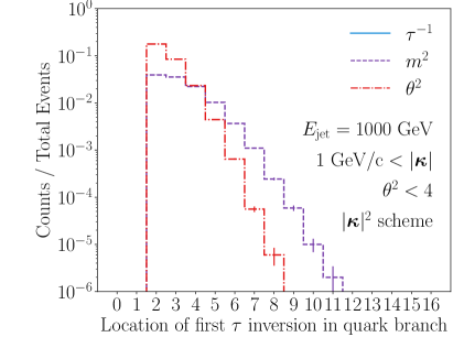
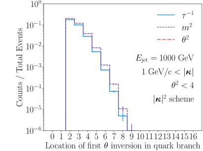
Figure 11: Location of the first inversion in formation time (left) and opening angle (right) along the quark branch of parton cascades generated according to the three ordering prescriptions in the momentum scheme, $\tau^{-1}$ (blue solid line), $m^{2}$ (purple dashed line), and $\theta^{2}$ (red dot-dashed line). Histograms expressed as fractions of the total number of events ($10^{6}$).

The significant fraction ($\gtrsim 10\%$) of events with at least one formation time or angular inversion in the quark branch raises the question about how these inversions affect the shower substructure. Aiming at exploring the potential interface between the shower and the evolving medium, we adopt two strategies for eliminating formation time inversions.

First, we simply exclude all events with at least one time inversion in their quark branch. The resulting Lund distributions are presented in figure 12 as ratios to the unmodified (or inclusive) samples. In these ratios, we observe minimal changes for the $m^{2}$-ordered cascades (top panel), with most of the modifications concentrated at wide angles and large $|\bm{\kappa}|$ values for the second and third splittings. This region corresponds to early values of $\tau$, which are more likely to exhibit inversions. For $\theta^{2}$-ordered cascades (bottom panel), the effect is significantly more pronounced, with the first splitting distribution being strongly suppressed in the low-$z$ region, corresponding to events with a large remaining phase space for the second splitting leading to a higher probability of time inversions. Additionally, the second and third splittings are suppressed for early formation times. In both cases, the post-hoc exclusion of formation time inversions significantly alters the Lund distributions. These modifications are of similar magnitude to the differences observed between ordering prescriptions.

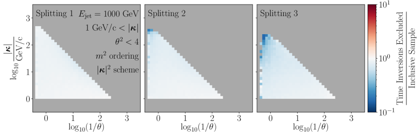
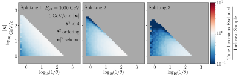
Figure 12: Lund plane distributions of the sample with a post-hoc exclusion of formation time inversions divided by the corresponding Lund distributions for the inclusive samples, for cascades ordered in $m^{2}$ (top), and $\theta^{2}$ (bottom) in the $|\bm{\kappa}|^{2}$ kinematic scheme. The first three quark-branch splittings were considered.

The second approach to eliminating formation time inversions consists of implementing a veto procedure during the shower generation. In this method, the splitting scale ($m^{2}$, $\theta^{2}$) and splitting fraction ($z$) are sampled as described in subsection 3.1.2, with the additional step of evaluating the formation time $\tau$ and comparing it to that of the previous splitting. If the trial splitting results in a time inversion, it is rejected, and the generation continues with a lower scale until a suitable splitting is found. The resulting Lund distributions, shown in figure 13, are presented as a ratio to the unmodified (inclusive) samples. In this approach, the first splitting distributions remain unaltered, since the no-inversion condition does not impose any restrictions on the first emission. However, the second and third splittings are noticeably modified. For $m^{2}$-ordered cascades the modification is concentrated in the wide-angle, large-$|\bm{\kappa}|$ corner of phase space, with fewer modifications in the collinear region than the post-hoc removal case. For $\theta$-ordered showers, we observe a sharp division between depleted and enhanced regions of the Lund plane, with their boundary given by a line of constant formation time, which increases with each splitting. While this veto-based implementation controls the modifications to the shower substructure better than the post-hoc removal of time inversions, the Lund distributions are still significantly altered, further increasing the inherent uncertainty to the double logarithmic approximation.

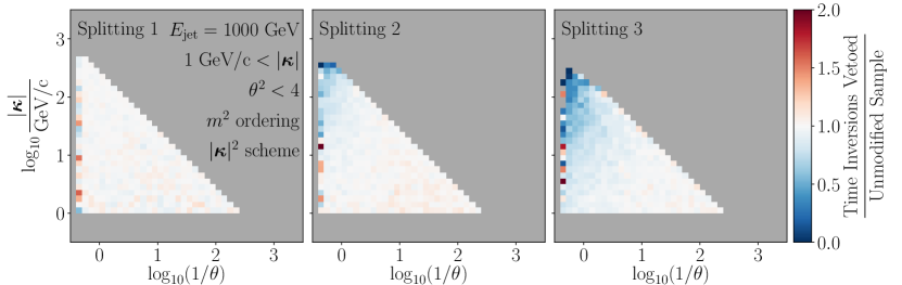
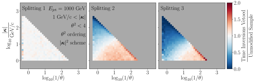
Figure 13: Ratio between Lund plane distributions of the sample with vetoed formation time inversions and the samples with unrestricted evolution, for cascades ordered in $m^{2}$ (top) and $\theta^{2}$ (bottom) in the $|\bm{\kappa}|^{2}$ kinematic scheme. The first three quark-branch splittings were considered.

We note that the results here refer solely to the $|\bm{\kappa}|^{2}$ scheme for the kinematic reconstruction, with inversions being absent in the $p^{2}$ scheme, see eqs. (43). However, since the latter is only one possible choice, this study still shows a relevant example of how time inversions may happen, and how removing them is non-trivial. For a further examination of the difference between the veto procedure and post-hoc exclusions, as well as the possibility of eliminating angular ordering violations, see appendix D.

5 Jet quenching studies

After exploring the uncertainties inherent to vacuum parton showers built upon the double logarithmic approximation, we turn to the influence of the ordering variable on the implementation of jet quenching models. Since any description of jet quenching requires a model for jet-medium interactions, a space-time picture of jet development is central to any such study, introducing another source of ambiguity in the implementation of a parton shower.

The most common approach, as exemplified by JEWEL Zapp:2008gi ; Zapp:2013vla , MATTER Majumder:2013re , and the Hybrid model Casalderrey-Solana:2014bpa , computes the formation time associated with each parton branching using the virtuality-dependent parametric form $\tau\propto E/p^{2}$ and evaluates the time-dependent medium properties by interpreting $\tau$ as the location of the splitting. A notable exception is the JetMed parton shower Caucal:2018dla ; Caucal:2020zcz , which orders in-medium parton splittings in coordinate light-cone time. Here, we simplify the jet-medium interactions into a series of phase-space cuts that discard events from the samples generated according to our three ordering prescriptions. In the analysis that follows, the discarded events are referred to as “quenched”, while the original events are referred to as a “vacuum” sample.

For the purposes of this study, these phase-space cuts are chosen according to a simplified colour-coherence picture for jet-medium interactions, where a splitting is considered inside the “quenched region” if its formation time is within the medium length, $L$, and above some decoherence timescale $t_{\rm dec}$ determined by the estimate

$$\hat{q}\tau>|\bm{\kappa}|^{2}\,\,\Longleftrightarrow\,\,\tau>\left(\hat{q}\theta^{2}\right)^{-1/3}=t_{\rm dec}(\theta)\,,$$ (46)

such that quenching is possible only if $t_{\rm dec}(\theta)<L$, a condition equivalent to the splitting angle being above the critical angle $\theta^{2}_{\rm c}=1/(\hat{q}L^{3})$, the parametric form given in Mehtar-Tani:2011vlz ; Casalderrey-Solana:2012evi . These two conditions can be incorporated in a quenching probability given by a piecewise function,

$$\mathcal{Q}=\Theta(t_{\rm dec}<\tau<L)\,,$$ (47)

where we have used the Heaviside function $\Theta(x)$, which returns $1$ when the condition $x$ is true, and $0$ otherwise.

Further, we stipulate two approaches for applying these quenching conditions to each event. In the first approach, referred to as “First Splitting”, an event is discarded if and only if the first splitting sampled from the no-emission probability (which does not necessarily have the shortest formation time) satisfies the quenching condition (47). The second option, denoted as “Full Shower”, involves discarding the event if at least one of the splittings along the quark branch of the cascade meets the quenching condition.

Finally, to assess the impact of formation time inversions on the outcome of this quenching model, we apply these conditions to three different “vacuum” samples. These samples consist of the full set generated according to the procedure outlined in section 3 (which includes all formation time inversions), as well as the two samples without time inversions studied in section 4.3, obtained either by the post-hoc exclusion of events or by implementing the time veto.

For simplicity, we restrict the results to a single quantity: the fraction of events eliminated by the quenching condition, $N_{\rm quenched}/N_{\rm vacuum}(\%)$. These quenching ratios are presented in figure 14 for three sets of medium parameters and for the three vacuum samples discussed above. Examining the results for the full, un-vetoed sample (left panel), we observe differences between ordering prescriptions, particularly for short-lived media, where $\theta$-ordered showers undergo slightly stronger quenching than their counterparts, at least for the hatched rectangles representing the “First Splitting” mode. This can be attributed to the first splitting in angular-ordered showers being more likely to populate the soft and wide-angle region of the Lund plane (see bottom panel of figure 5), which falls inside the quenched region of phase space (see appendix A).

When this exercise is repeated for the other two samples (middle and right panels), the differences between algorithms remain mostly unchanged in the “First Splitting” mode — a reflection of the fact that the first splitting distributions are not significantly altered by the exclusion of time inversions, and, in fact, remain completely unaltered in the case of the time veto shown on the right panel. However, in the “Full Shower” mode (empty rectangles), the quenched fractions exhibit significant differences between the angular-ordered shower and the other two algorithms in the case of post-hoc exclusion of time inversions (middle panel). This arises due to the strong bias towards later formation times, which shifts the event into the quenched region of phase space, an effect not observed in the vetoed sample. An analogous study, considering the exclusion of angular inversions, is presented in appendix E, where even larger differences between ordering prescriptions are found.

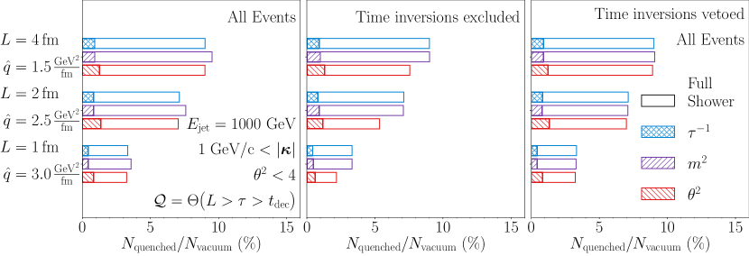
Figure 14: Percentage of events obeying the quenching condition with different values of $(L,\hat{q})$ in equation (47) in samples generated according to formation time (blue crossed), invariant mass (purple slanted), and angle (red counter-slanted) ordering prescriptions. Hatched rectangles correspond to the “First Splitting” mode and empty rectangles to the “Full Shower”. Vacuum samples consisting of all events (left panel), only events with no inversion (centre panel), and inversion-vetoed events (right panel).

To conclude, we note that even in our highly simplified framework for jet quenching, the choice of the ordering variable in the parton shower produces noticeable variations in the quenching results. This is a natural consequence of the lack of direct connection between certain ordering variables and the space-time picture of the medium. Notably, the differences are relatively larger for the first splitting and in thin media. The impact of varying the pseudo-quenching model, jet energy, hadronisation scale, and the kinematic scheme on the quenching ratios is analysed in appendix E.

6 Conclusions

In this study, we establish a consistent definition for parton formation times in a two-gluon emission process within the phase-space region where the double logarithmic approximation is valid, connecting these formation times with the angular ordering conditions known from colour-coherence arguments.

In order to explore the differences between ordering prescriptions within the Double Logarithmic Approximation, we build a Monte Carlo parton shower ordered in three different kinematic variables: the invariant mass, the formation time, and the opening angle of the parton splittings. We further consider two sets of proxies (or schemes) for these variables, either in terms of the virtual mass or the relative transverse momentum of the daughter pairs. By generating quark-initiated cascades and computing the main branch Lund plane distributions, we find that the choice of ordering prescription has a larger impact than the choice of the scheme, with the differences being primarily located in the large-angle region.

Further, we investigate the possibility of assigning a spacetime structure to a parton cascade through the formation time kinematic variable. We test two procedures to ensure a strictly increasing time: either by requiring this condition during the generation of the cascade or by post-hoc excluding events that violate time ordering. We find that both of these procedures significantly alter the Lund plane distributions for invariant-mass and angular-ordered cascades. Finally, we implement a simple decoherence-based jet quenching model to the event samples generated with our three parton showers and both procedures to avoid time-ordering violations. In computing the fractions of quenched events for all these cases, we observe some dependence on the ordering prescription, particularly for the first splitting and for thin media.

Our work highlights the uncertainties stemming for interfacing a parton cascade with a medium defined in space-time. These uncertainties must be taken into account when comparing Monte Carlo jet quenching models with experimental data, which aim to establish relative contributions of different effects (radiative and collisional energy losses, medium response, etc.) and ultimately provide a quantitative characterisation of the medium. We conclude that a major step in precision will require either further first-principle studies to clarify the relation between the momentum and space-time descriptions of in-medium parton cascades or the development of parton cascades formulated purely in space-time.

Appendix A Lund plane conventions

Over the course of this manuscript, we describe the phase space for parton emissions by specifying the relative transverse momentum of the daughter partons $|\bm{\kappa}|$ and the angular proxy $\theta$, represented in a Lund plane Dreyer:2018nbf as depicted in figure 15 (left). In this Lund plane configuration, wide emissions are located further to the right, while emissions closer to the hadronisation scale $|\bm{\kappa}|\to\Lambda$ are located towards the lower part of the diagram. Furthermore, according to eqs. (25), the diagonal directions are associated with increasing values of formation time $\tau$ and $Ez(1-z)$. For a fixed splitting, the latter approximately corresponds in the soft limit to increasing values of the energy fraction $z$. In this Lund configuration, the phase-space limits of a parton splitting draw a right triangle consisting of a left bound set by the maximum angular proxy $\theta^{2}<4$, a lower bound set by the hadronisation scale $|\bm{\kappa}|>\Lambda$, and a diagonal bound set by $z(1-z)<1/4$ (disregarding any depletion of the mother’s energy $E$).

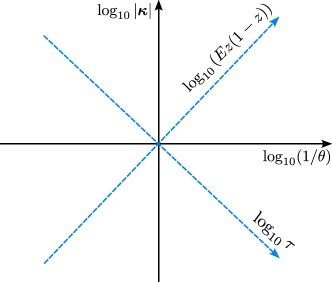
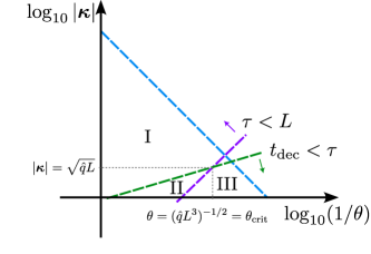
Figure 15: Left: Lund plane configuration used throughout this study to represent the available phase space for parton emissions. Right: Different phase-space regions relevant for the pseudo-quenching models, including in-medium vacuum-like emissions (region I), broadening dominated splittings (region II), and splittings outside of the medium (region III).

In the main text we introduce two different kinematic schemes, as well as two different Lund configurations, consisting of the variable pairs $(\theta_{*},\bm{\kappa}_{*})$ and $(\theta,\bm{\kappa})$. These are related by

$$\theta_{*}=\frac{|\bm{\kappa}_{*}|}{Ez(1-z)}\,,\qquad\theta=\frac{|\bm{\kappa}|}{Ez(1-z)}\,.$$ (48)

When considering these Lund plane configurations, it is worth keeping in mind that

$$|\bm{\kappa}|/\theta=|\bm{\kappa}_{*}|/\theta_{*}=Ez(1-z)\,,$$ (49)

meaning that the main diagonal direction can be taken to represent the hardness (in energy) of a splitting in both Lund configurations and for both schemes.

Additionally, we have

$$|\bm{\kappa}_{*}|\,\theta_{*}=\frac{p^{2}}{E}=\tau^{-1}_{*}\,,\qquad|\bm{\kappa}|\,\theta=\frac{|\bm{\kappa}|^{2}}{Ez(1-z)}=\tau^{-1}\,,$$ (50)

showing that in both pairs of variables, the anti-diagonal direction corresponds to some definition of inverse formation time.

Section 5 focuses on the impact of the vacuum ordering prescription on jet quenching phenomena by exploring simplified pseudo-quenching models, where cascades are discarded from the vacuum samples according to the region of phase space they occupy. The right panel of figure 15 illustrates the phase-space bounds for a vacuum sample (in blue), the medium length constraint $\tau<L$ (in purple), and the decoherence time bound $t_{\rm dec}=(\hat{q}\theta^{2})^{-1/3}$ (in green). This allows us to identify three different regions: vacuum-like splittings inside the medium ($\tau<t_{\rm dec},L$); broadening-dominated splitting ($t_{\rm dec}<\tau<L$); and splittings occurring outside of the medium ($L<\tau$), respectively labelled as I, II, and III. Additionally, a critical angle $\theta^{2}_{\rm crit}$ is identified, corresponding to emissions where the decoherence time is equal to the length of the medium. The pseudo-quenching model considered in section 5 is understood as eliminating cascades whose quark-branch splittings fall into region II.

Appendix B One-dimensional distributions

This appendix begins by summarising the one-dimensional distributions for the relative transverse momentum $|\bm{\kappa}|$, the angular ordering variable $\theta^{2}$, and the light-cone momentum fraction $z$ (sampled from the splitting kernel). These distributions are shown in figure 16 for the first three splittings along the quark branch of cascades generated according to the $|\bm{\kappa}|^{2}$ scheme.

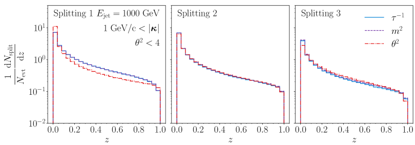
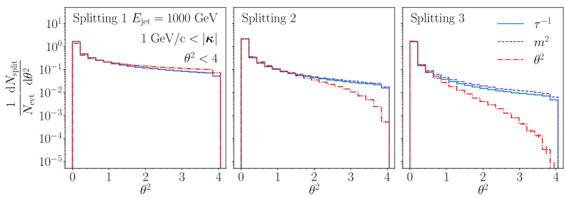
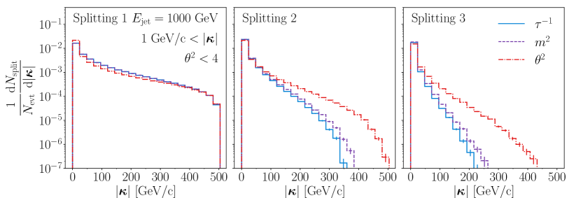
Figure 16: Kinematic distributions for parton cascades generated according to the transverse momentum scheme, for three different ordering prescriptions: $\tau^{-1}$ (blue solid line), $m^{2}$ (purple dashed line), and $\theta^{2}$ (red dash-dotted line). Each panel from left to right corresponds to the first, second, and third quark-initiated splitting in the cascade. Distributions of the light-cone energy fraction $z$ (top), the squared angular ordering variable (middle), and the relative transverse momentum (bottom) are presented.

Firstly, we note the similarity between the energy fraction distributions (top panels), despite $\theta^{2}$-ordered cascades favouring lower energy fractions early in the shower and flattening faster than the other two ordering prescriptions. This is understood as a consequence of the different dependence of the soft regulator on the splitting scale, as discussed in the main text. When examining the distributions of the squared angular ordering variable $\theta^{2}$ (middle panels), we note a marked difference between ordering prescriptions, with angular ordering cascades showing a narrowing effect as the shower advances, as expected from the strong ordering conditions. The other ordering prescriptions, on the other hand, fill the available phase space for the $\theta^{2}$ variable in an approximately uniform way for all splittings. Finally, examining the distributions of relative transverse momentum (bottom panels), we see that despite starting in similar configurations for all three ordering prescriptions, the distributions quickly diverge and even develop different endpoints. This deviation results from the different depletion of phase space for the angular proxy $\theta^{2}$ and the different rates at which the splitting function $z$ flattens out, which also causes different rates for the depletion of the quark’s energy $E$.

To provide a clearer quantitative comparison between the effects of changing ordering variables and those of changing the kinematic scheme, we computed various distributions as ratios to their counterparts derived from time-ordered cascades in the momentum scheme.

In figure 17, we present such ratios for the number of splittings along the quark branch. Consistently with the main text, most differences are observed in the tails of the distributions. Notably, mass-ordered cascades are generally longer, being approximately four times more likely to exhibit ten splittings compared to the baseline. In contrast,the $p^{2}$ scheme tends to produce shorter cascades being about five times less likely to show ten splittings than the chosen baseline. These effects arise from how the phase space is assigned in each implementation: mass-ordered cascades have a power-enhanced dependence on the splitting scale compared to the time-ordered case, while the $p^{2}$-scheme, which includes an additional veto, biases splittings towards the hadronization scale, effectively shortening the cascade.

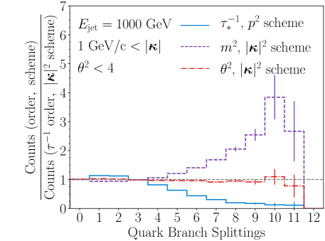
Figure 17: Number of quark-initiated splittings in $\tau^{-1}_{*}$-ordered, mass scheme (blue solid line); $m^{2}$-ordered, momentum scheme (purple dashed line); and $\theta^{2}$-ordered, momentum scheme (red dash-dotted line), as a ratio to the same quantity for time-ordered cascades generated in the $|\bm{\kappa}|^{2}$ scheme.

We further note the differences between the $|\bm{\kappa}|$ and $z$ spectra, as depicted in figure 18. A key observation is the consistent agreement between the first splitting distributions of $\tau^{-1}$ and $m^{2}$ ordered cascades. This consistency is expected because their only difference lies in an additional factor of the incoming quark energy, which is fixed for the first splitting. Conversely, we observe a notable disagreement between angular-ordered cascades and the time-ordered case, with angular ordering favouring more asymmetric splittings due to its smaller infrared cutoff. Finally, we contrast the agreement between schemes for time ordered cascades for the $z$ spectrum, a directly sampled quantity, with the disagreement in the $|\bm{\kappa}|$ spectrum, which involves the scales of subsequent splittings. This highlights that major differences between schemes arise from different definitions of kinematic variables, at least in the case of time-ordered cascades.

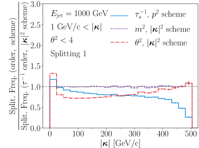
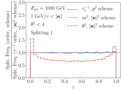
Figure 18: Ratio of kinematic distributions between different ordering prescriptions and schemes and time-ordered cascades in the $|\bm{\kappa}|^{2}$ scheme. This includes $\tau^{-1}_{*}$-ordered, $p^{2}$-scheme (blue solid line); $m^{2}$-ordered, $|\bm{\kappa}|^{2}$-scheme (purple dashed line); and $\theta^{2}$-ordered, momentum scheme (red dash-dotted line). Left: Relative transverse $|\bm{\kappa}|^{2}$ distributions. Right: Splitting fraction distributions. Numerator and denominator distributions are not self-normalised before the ratio.

Appendix C Different orderings for the mass scheme

This appendix explores different ordering prescriptions in the “ $p^{2}$ scheme”. We start by analysing the Lund ratios between these ordering prescriptions in this kinematic scheme, as shown in figure 19.

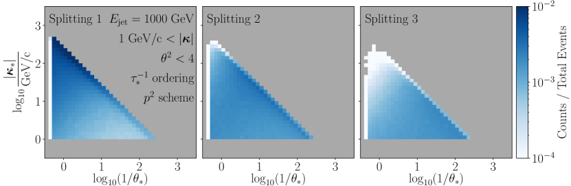
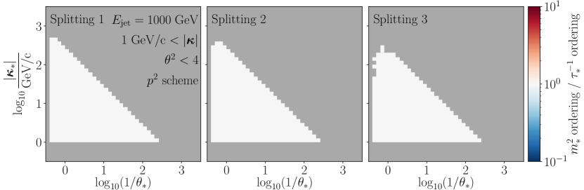
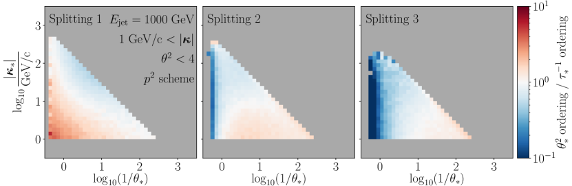
Figure 19: Lund plane distributions in the $(\theta_{*},\bm{\kappa}_{*})$ configuration for the first three $q\to qg$ splittings of cascades generated according to the “$p^{2}$ scheme”. Top: Densities for $\tau^{-1}_{*}$-ordered cascades. Bins below the minimum are shown in white and empty bins shown in grey. All densities are normalised to the total number of events. Middle: Ratio between $m_{*}^{2}$ and $\tau^{-1}_{*}$ ordered cascades. Bottom: Ratio between $\theta_{*}^{2}$ and $\tau^{-1}_{*}$ ordered cascades.

While the broad features of the time-ordered samples are the same in both schemes, a striking similarity is observed between $m^{2}$ and $\tau^{-1}$ ordered cascades in this kinematic scheme, with their ratio being exactly unity throughout the entire phase space (see middle panel). This similarity even holds on an event-by-event basis, since the veto procedure necessary to ensure $|\bm{\kappa}|>\Lambda$ supersedes any time-ordering prescription, as discussed at the end of section 3.2. Since both samples are constrained into a phase-space region that enforces time ordering, their densities are identical. For the angular-ordered case, depicted in the bottom panel, the first splitting exhibits the same features as in the momentum scheme (see figure 5), while subsequent splittings show milder differences between orderings, albeit distributed over a larger region of phase space. Repeating this analysis in the Lund Plane configuration given by $(\theta,\bm{\kappa})$ produces largely similar results. Overall, these findings highlight the stronger constraints inherent in this kinematic scheme, which tend to minimise differences between orderings.

Next, we present the Lund plane ratios between the kinematic schemes for both $m_{*}^{2}$ and $\theta_{*}^{2}$-ordered cascades in figures 20 and 21, respectively. These figures complement the results discussed in section 4.2.

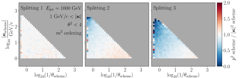
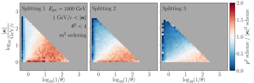
Figure 20: Ratio between Lund plane distributions in both kinematic schemes, for mass-ordered cascades. Bins where the denominator vanishes are shown in grey. Top: The distribution corresponding to each scheme was computed for the variables most natural to each scheme. Bottom: Both distributions were computed using the variables $(\theta,|\bm{\kappa}|)$.

In these figures, the top panels display the Lund configurations using the variables most natural to each scheme $(\theta_{\rm scheme},\bm{\kappa}_{\rm scheme})$, while the bottom panels use the “kinematic variables” $(\theta,\bm{\kappa})$. In general, for the first Lund configuration, switching from the “$p^{2}$ scheme” to the “$|\bm{\kappa}|^{2}$ scheme” corresponds to a time veto, suppressing early splittings and enhancing later ones, particularly in the case of $\theta_{*}^{2}$-ordered cascades (see figure 21). This effect is explained by the veto procedure ensuring $|\bm{\kappa}|>\Lambda$, as discussed at the end of section 3.2. For the second Lund configuration (bottom panels of figures 20 and 21), the preference of low $|\bm{\kappa}|$ and $\theta$ splittings is more pronounced for mass-ordered cascades. In contrast, the ratios for angular-ordered cascades appear similar.

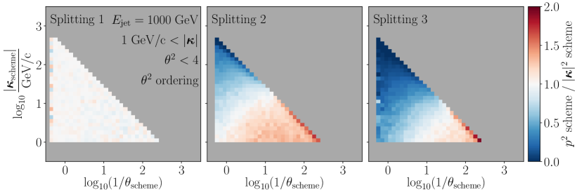
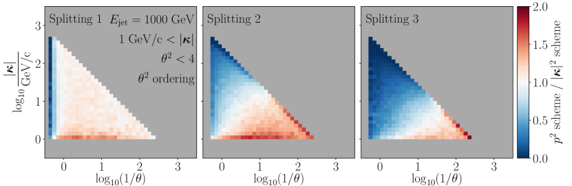
Figure 21: Ratio between Lund plane distributions in both kinematic schemes, for angular ordered cascades. Bins where the denominator vanishes are shown in grey. Top: The distribution corresponding to each scheme was computed over the variables most natural to each scheme. Bottom: Both distributions computed over the $(\theta,|\bm{\kappa}|)$.

In summary, the results in this section highlight that the “$p^{2}$ scheme” effectively delays emissions according to its definition of formation time as $\tau_{*}=E/p^{2}$, and that it constrains the parton shower development more strongly than the “$|\bm{\kappa}|^{2}$ scheme”.

Appendix D Comparing exclusions and vetos

In this appendix, we explore the effects of vetoing and excluding inversions in two ordering variables, formation time $t_{\rm form}$ and opening angle $\theta^{2}$. Specifically, the top panel of figure 22 shows ratios between two different samples: the formation time sample with all events that have at least one $\theta^{2}$-ordering violation along the quark excluded, divided by the angular-ordered sample with all events that have at least one formation-time ordering violation along the quark branch excluded. Notably, this ratio is compatible with unity across the entire phase space for the three first splittings, with some statistical fluctuations observed in the case of the third splitting in the region of large angles and small formation times, where events are likely to be excluded from the numerator or denominator, respectively. We also note that this ratio is close to, but slightly larger than one, reflecting the fact that there are slightly more angular inversions in the $\tau^{-1}$-ordered sample ($\sim$ 37%) compared formation-time inversions in the $\theta^{2}$-ordered sample ($\sim$ 29%) (cf. figure 11).

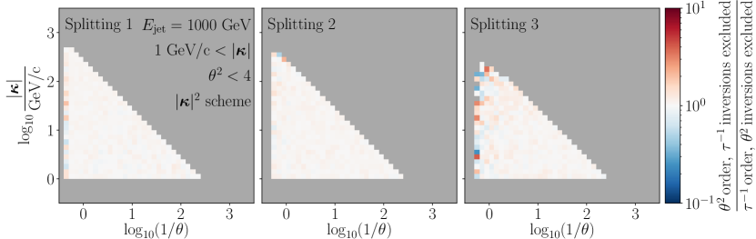
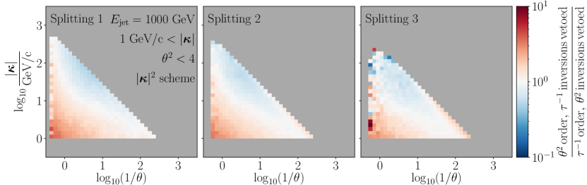
Figure 22: Ratios of Lund plane densities for the three first quark-initiated splittings of cascades generated according to the “$|\bm{\kappa}|^{2}$ scheme”. Top: Ratio between the $\tau^{-1}$-ordered sample with angular inversions excluded post-hoc and the $\theta^{2}$-ordered sample with time inversions excluded post-hoc. Bottom: Ratio between the $\tau^{-1}$-ordered sample where angular inversions are vetoed and the $\theta^{2}$-ordered sample where time inversions are vetoed.

When repeating this exercise using a veto procedure instead of a post-hoc exclusion, i.e. by treating either time or angle inversions as unresolved splittings, one obtains the Lund ratios in the bottom panel of figure 22, which depict rather strong modifications, especially towards softer $z$ distributions. This analysis reveals, that while the veto procedure preserves the first splitting distributions in the unmodified sample, the post-hoc exclusion procedure respects the strong ordering in different variables. As such, there is no clear advantage to either method for preventing inversions in some shower variable.

Appendix E Further results in jet quenching

Having explored a rather simplistic model for medium-jet interactions in section 5, this appendix examines how the fractions of quenched events are affected by varying the quenching condition, jet energies, and hadronisation scale, as well as the vetoes inherent to the kinematic scheme. Both in this appendix and the main text, the relative statistical uncertainties on the quenching ratios are $\leq 4\times 10^{-3}$ and have not been displayed.

E.1 Different quenching conditions

Besides the quenching condition studied in the main text, we consider two others:

$$\mathcal{Q} =\Theta(t_{\rm dec}<\tau<L)\,,$$ (51a)

$$\mathcal{Q} =\Theta(\tau<L)\,\exp\{-\tau^{3}/t^{3}_{\rm dec}\}\,,\,$$ (51b)

$$\mathcal{Q} =\Theta(\tau<L)\times\Theta(\hat{q}L<|\bm{\kappa}|^{2})\,,$$ (51c)

where the first equation reflects the criterion employed in the main text (cf. eq.(47)), the second reflects the parametric dependence on the “decoherence rate” found in Mehtar-Tani:2011vlz , and the third corresponds to a broader restriction of the relative transverse momentum being above the inverse saturation scale of the static medium $Q^{-2}_{\rm sat}\equiv\hat{q}L$. The main difference between these latter two conditions and the one implemented in the main text is their treatment of the low $|\bm{\kappa}|$, high $\theta$ region of the Lund plane, with the third condition suppressing this region more significantly .

To ensure that the dependence of the quenching fractions on the ordering variable is not merely a consequence of regions of phase space dominated by wide-angle cascades, we introduce a “jet radius” parameter $R_{\rm max}$ and restrict the vacuum sample so that each $q\to qg$ splitting obeys $\theta<R_{\rm max}$. This condition is expected to mimic the effects of a jet cone, thereby restricting our analysis to the collinear region of the Lund Plane.

The resulting quenching ratios for the three probabilities in eqs. (51) and for three different values of $R_{\rm max}$ are presented in figure 23. The top panel corresponds to a short-lived, dense medium ($L=$1\text{\,}\mathrm{f}\mathrm{m}$$, $\hat{q}=$3\text{\,}\mathrm{G}\mathrm{e}\mathrm{V}^{2}\mathrm{/}\mathrm{f}\mathrm{m}$$), while the bottom panel relates to longer-lived, dilute medium ($L=$4\text{\,}\mathrm{f}\mathrm{m}$$, $\hat{q}=$1.5\text{\,}\mathrm{G}\mathrm{e}\mathrm{V}^{2}\mathrm{/}\mathrm{f}\mathrm{m}$$). As in the main text, full bars correspond to applying the condition only to the first splitting, and hollow bars reflect its application to the entire quark branch. Notably, the behaviour of the quenching ratios with the jet radius parameter $R_{\rm max}$ differs between short-lived and long-lived media. Namely, in the short-lived medium, the “Full Shower” ratio increases with $R_{\rm max}$, whereas in the longer-lived medium, the “First Splitting” quenching weights decrease as the jet radius increases. This can be attributed to the interplay of two effects: wider cascades are both more likely to contain early splittings with low $\tau$ and to present shorter decoherence times. In the $L=1\,{\rm fm}$ case, the first factor plays a key role in increasing the quenching ratios for wide splittings, while in the $L=4\,{\rm fm}$ case, the second factor becomes more relevant, as most first splittings are likely to occur inside of the medium. An exception is seen with the third model (right panel), which does not depend on a decoherence time scale, and therefore behaves differently.

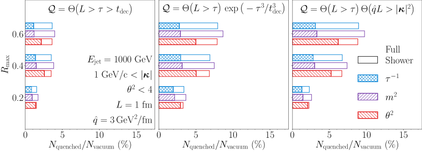
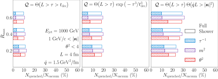
Figure 23: Percentage of events obeying the quenching conditions in eqs. (51) in samples generated according to formation time (blue), invariant mass (purple), and angle (red) ordering prescriptions. The Hatched rectangles correspond to the “First Splitting” mode, while the empty rectangles to the “Full Shower”. All samples were restricted such that quark-branch splittings had $\theta<R_{\rm max}$ before quenching. The top panel correspond to ($L=$1\text{\,}\mathrm{f}\mathrm{m}$$, $\hat{q}=$3\text{\,}\mathrm{G}\mathrm{e}\mathrm{V}^{2}\mathrm{/}\mathrm{f}\mathrm{m}$$), and the bottom panel to ($L=$4\text{\,}\mathrm{f}\mathrm{m}$$, $\hat{q}=$1.5\text{\,}\mathrm{G}\mathrm{e}\mathrm{V}^{2}\mathrm{/}\mathrm{f}\mathrm{m}$$).

The main result of this exercise is that the dependence on the ordering prescription persists across all three models and values of $R_{\rm max}$, especially when focusing in the first splitting. The fact that differences between ordering variables persist even when jets are restricted to the collinear region (e.g. $R_{\rm max}=0.2$) — where Lund plane ratios between different ordering prescriptions approach unity, as depicted in figure 5 — can be better understood by considering these rations for the restricted samples, as shown in figure 24. Notably, although all samples have been restricted to the region where the ratios were previously compatible with unity, the differences between algorithms, previously located in the wide-angle region of phase space, have reappeared near $\theta\sim R_{\rm max}$. This suggests that the Lund planes appear simply rescaled. This finding clarifies our earlier results: even though ordering prescriptions may seem to agree in the collinear region, once all samples are restricted to small angles by the same procedure, the Lund plane ratios continue to reflect differences between algorithms.

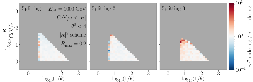
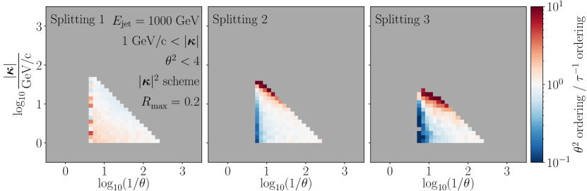
Figure 24: Lund plane distributions in the $(\theta,\bm{\kappa})$ configuration for the first three $q\to qg$ splittings of cascades generated according to the “$|\bm{\kappa}|^{2}$ scheme”. The samples restricted to only those events where all $\theta<R_{\rm max}=0.2$. Top: Ratio between $m^{2}$ and $\tau^{-1}$-ordered cascades. Bottom: Ratio between $\theta^{2}$ and $\tau^{-1}$-ordered cascades.

We finally note that an alternative approach to mimic the jet cone was tested. Instead of discarding any events with $\theta>R_{\rm max}$, this method involved discarding splittings with an angle above a cutoff $r_{\rm g}$, thus keeping the event but potentially the shower history. The results obtained with this approach were qualitatively similar to those described previously, albeit with marginally smaller quenching ratios.

E.2 Different starting and stopping scales

We now examine the effects of varying the starting and stopping scales used to generate the vacuum samples. In figure 25, we represent the results of the main text (left panel), along with the equivalent results for a lower jet energy of $E_{\rm jet}=$500\text{\,}\mathrm{G}\mathrm{e}\mathrm{V}$$ (middle panel), and a lower hadronisation scale of $\Lambda=$0.1\text{\,}\mathrm{G}\mathrm{e}\mathrm{V}\mathrm{/}\mathrm{c}$$ (right panel). The quenching probability corresponds to that of the main text, see eq. (47), and the medium parameters correspond to the short-lived and dense medium employed in the previous section.

As before, the differences between ordering variables remain. We observe some disagreement between the three different sets of phase-space values in the wider sample ($R_{\rm max}$ = 0.6), with results converging for narrower samples. This also confirms that while the parton shower is not generally independent of the factorisation scales chosen by the user, this dependence decreases as one approaches the collinear limit. Finally, when this exercise is carried out for different medium parameters, such as ($L=$4\text{\,}\mathrm{f}\mathrm{m}$$, $\hat{q}=$1.5\text{\,}\mathrm{G}\mathrm{e}\mathrm{V}^{2}\mathrm{/}\mathrm{f}\mathrm{m}$$), one observes the same trends as in the previous section.

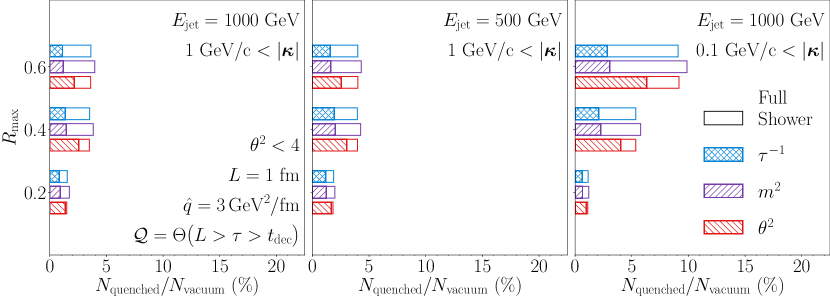
Figure 25: Percentage of events obeying the quenching condition defined by the first equation in eqs. (51) for samples generated according to formation-time (blue), invariant-mass (purple), and angular (red) ordering prescriptions. Hatched rectangles correspond to the “First Splitting” mode, while empty rectangles to the “Full Shower” mode. Different panels correspond to differently chosen jet energies ($E_{\rm jet}$) and hadronisation scales for the vacuum samples. Prior to applying the quenching condition, the samples were restricted to quark-branch splittings with $\theta<R_{\rm max}$. The medium parameters used are $L=$1\text{\,}\mathrm{f}\mathrm{m}$$, and $\hat{q}=$3\text{\,}\mathrm{G}\mathrm{e}\mathrm{V}^{2}\mathrm{/}\mathrm{f}\mathrm{m}$$.

E.3 Sensitivity to angular inversions

It is also worth considering is the role of angular inversions in our pseudo-quenching model. To this end, we repeat the calculations that led to figure 14, but this time by preventing inversions in angle rather than formation time. The results are shown in figure 26. Here, we note that the source of differences between algorithms is not solely the presence of angular ordering, although it does contribute to the sensitivity to jet colour decoherence. When angular inversions along the quark branch are excluded post-hoc (middle panel), significant differences between the different orderings are observed in the “Full Shower” mode (empty rectangles), as parton cascades are biased towards configurations where later splittings are more collinear. When these inversions are prevented by veto (right panel), a similar behaviour emerges, although in this case the differences are already present in the “First Splitting” mode.

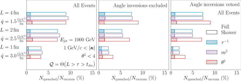
Figure 26: Percentage of events satisfying the quenching condition in eq. (47) for different values of $L$ and $\hat{q}$ and for samples generated according to formation-time (blue), invariant-mass (purple), and angular (red) ordering prescriptions. Results on vacuum samples consisting of all events (left panel), events with angular inversions excluded post-hoc (centre panel), and events with vetoed angular inversions (right panel). Hatched rectangles correspond to the “First Splitting” mode, while empty rectangles to the “Full Shower”.

Overall we see how a simple model for jet decoherence is sensitive to the choices of strong ordering prescription and of how angular ordering is enforced.

E.4 Different kinematic scheme

Finally and for completeness, we reiterate our pseudo-quenching exercise for different kinematic reconstruction schemes. The results are shown in figure 27, with quantitative differences evident for all three models across all values of $R_{\rm max}$. Notably, the $|\bm{\kappa}|^{2}$-scheme (blue crossed) exhibits lower quenching ratios than the $p^{2}$-scheme (blue squared). This result is somewhat counter-intuitive, as one might expect the time veto inherent to the $p^{2}$-scheme to effectively push emissions outside the medium. However, due to the bias towards lower transverse momentum in this scheme, the quenching ratios tend to be slightly larger, regardless of $R_{\rm max}$.

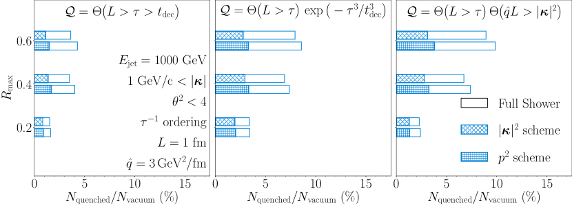
Figure 27: Percentage of events obeying the quenching condition in eqs. (51) for samples generated according to formation-time ordering prescription in the $|\bm{\kappa}|^{2}$ (blue crossed) and $p^{2}$ (blue squared) schemes. Prior to applying the quenching condition, the samples were restricted to quark-branch splittings with $\theta<R_{\rm max}$. The medium parameters used are $L=$1\text{\,}\mathrm{f}\mathrm{m}$$, and $\hat{q}=$3\text{\,}\mathrm{G}\mathrm{e}\mathrm{V}^{2}\mathrm{/}\mathrm{f}\mathrm{m}$$.

References

- (1) J.M. Campbell et al., Event Generators for High-Energy Physics Experiments, in Snowmass 2021, 3, 2022 [2203.11110].
- (2) L. Apolinário, Y.-T. Chien and L. Cunqueiro Mendez, Jet substructure, Int. J. Mod. Phys. E 33 (2024) 2430003.
- (3) G. Bewick, S. Ferrario Ravasio, P. Richardson and M.H. Seymour, Logarithmic accuracy of angular-ordered parton showers, JHEP 04 (2020) 019 [1904.11866].
- (4) M. Dasgupta, F.A. Dreyer, K. Hamilton, P.F. Monni, G.P. Salam and G. Soyez, Parton showers beyond leading logarithmic accuracy, Phys. Rev. Lett. 125 (2020) 052002 [2002.11114].
- (5) J.R. Forshaw, J. Holguin and S. Plätzer, Building a consistent parton shower, JHEP 09 (2020) 014 [2003.06400].
- (6) Z. Nagy and D.E. Soper, Summations of large logarithms by parton showers, Phys. Rev. D 104 (2021) 054049 [2011.04773].
- (7) Z. Nagy and D.E. Soper, Summations by parton showers of large logarithms in electron-positron annihilation, 2011.04777.
- (8) G. Bewick, S. Ferrario Ravasio, P. Richardson and M.H. Seymour, Initial state radiation in the Herwig 7 angular-ordered parton shower, JHEP 01 (2022) 026 [2107.04051].
- (9) M. van Beekveld, S. Ferrario Ravasio, K. Hamilton, G.P. Salam, A. Soto-Ontoso, G. Soyez et al., PanScales showers for hadron collisions: all-order validation, JHEP 11 (2022) 020 [2207.09467].
- (10) F. Herren, S. Höche, F. Krauss, D. Reichelt and M. Schoenherr, A new approach to color-coherent parton evolution, JHEP 10 (2023) 091 [2208.06057].
- (11) M. van Beekveld and S. Ferrario Ravasio, Next-to-leading-logarithmic PanScales showers for Deep Inelastic Scattering and Vector Boson Fusion, 2305.08645.
- (12) S. Ferrario Ravasio, K. Hamilton, A. Karlberg, G.P. Salam, L. Scyboz and G. Soyez, Parton Showering with Higher Logarithmic Accuracy for Soft Emissions, Phys. Rev. Lett. 131 (2023) 161906 [2307.11142].
- (13) M. van Beekveld et al., A new standard for the logarithmic accuracy of parton showers, 2406.02661.
- (14) Y. Mehtar-Tani, J.G. Milhano and K. Tywoniuk, Jet physics in heavy-ion collisions, Int. J. Mod. Phys. A 28 (2013) 1340013 [1302.2579].
- (15) J.-P. Blaizot and Y. Mehtar-Tani, Jet Structure in Heavy Ion Collisions, Int. J. Mod. Phys. E 24 (2015) 1530012 [1503.05958].
- (16) L. Apolinário, Y.-J. Lee and M. Winn, Heavy quarks and jets as probes of the QGP, Prog. Part. Nucl. Phys. 127 (2022) 103990 [2203.16352].
- (17) I.P. Lokhtin and A.M. Snigirev, A Model of jet quenching in ultrarelativistic heavy ion collisions and high-p(T) hadron spectra at RHIC, Eur. Phys. J. C 45 (2006) 211 [hep-ph/0506189].
- (18) B. Schenke, C. Gale and S. Jeon, MARTINI: An Event generator for relativistic heavy-ion collisions, Phys. Rev. C 80 (2009) 054913 [0909.2037].
- (19) W.-T. Deng, X.-N. Wang and R. Xu, Hadron production in p+p, p+Pb, and Pb+Pb collisions with the HIJING 2.0 model at energies available at the CERN Large Hadron Collider, Phys. Rev. C 83 (2011) 014915 [1008.1841].
- (20) J. Casalderrey-Solana, D.C. Gulhan, J.G. Milhano, D. Pablos and K. Rajagopal, A Hybrid Strong/Weak Coupling Approach to Jet Quenching, JHEP 10 (2014) 019 [1405.3864].
- (21) P. Caucal, E. Iancu, A.H. Mueller and G. Soyez, Vacuum-like jet fragmentation in a dense QCD medium, Phys. Rev. Lett. 120 (2018) 232001 [1801.09703].
- (22) T. Luo, Y. He, S. Cao and X.-N. Wang, Linear Boltzmann transport for jet propagation in the quark-gluon plasma: Inelastic processes and jet modification, 2306.13742.
- (23) N. Armesto, L. Cunqueiro and C.A. Salgado, Q-PYTHIA: A Medium-modified implementation of final state radiation, Eur. Phys. J. C 63 (2009) 679 [0907.1014].
- (24) K.C. Zapp, JEWEL 2.0.0: directions for use, Eur. Phys. J. C 74 (2014) 2762 [1311.0048].
- (25) J.H. Putschke et al., The JETSCAPE framework, 1903.07706.
- (26) A. Takacs, D. Pablos and K. Tywoniuk, Resolving the spacetime structure of jets with medium, PoS HardProbes2020 (2021) 161 [2009.02936].
- (27) Z. Nagy and D.E. Soper, On the transverse momentum in Z-boson production in a virtuality ordered parton shower, JHEP 03 (2010) 097 [0912.4534].
- (28) Z. Nagy and D.E. Soper, Ordering variable for parton showers, JHEP 06 (2014) 178 [1401.6366].
- (29) M. van Beekveld, S. Ferrario Ravasio, G.P. Salam, A. Soto-Ontoso, G. Soyez and R. Verheyen, PanScales parton showers for hadron collisions: formulation and fixed-order studies, JHEP 11 (2022) 019 [2205.02237].
- (30) F.A. Dreyer, G.P. Salam and G. Soyez, The Lund Jet Plane, JHEP 12 (2018) 064 [1807.04758].
- (31) V.N. Gribov and L.N. Lipatov, Deep inelastic e p scattering in perturbation theory, Sov. J. Nucl. Phys. 15 (1972) 438.
- (32) V.N. Gribov and L.N. Lipatov, pair annihilation and deep inelastic e p scattering in perturbation theory, Sov. J. Nucl. Phys. 15 (1972) 675.
- (33) G. Altarelli and G. Parisi, Asymptotic Freedom in Parton Language, Nucl. Phys. B126 (1977) 298.
- (34) Y.L. Dokshitzer, Calculation of the Structure Functions for Deep Inelastic Scattering and Annihilation by Perturbation Theory in Quantum Chromodynamics., Sov. Phys. JETP 46 (1977) 641.
- (35) C. Bierlich et al., A comprehensive guide to the physics and usage of PYTHIA 8.3, 2203.11601.
- (36) L. Lönnblad, Fooling Around with the Sudakov Veto Algorithm, Eur. Phys. J. C 73 (2013) 2350 [1211.7204].
- (37) B.R. Webber, Monte Carlo Simulation of Hard Hadronic Processes, Ann. Rev. Nucl. Part. Sci. 36 (1986) 253.
- (38) R.K. Ellis, W.J. Stirling and B.R. Webber, QCD and collider physics, vol. 8, Cambridge University Press (2, 2011), 10.1017/CBO9780511628788.
- (39) K. Zapp, G. Ingelman, J. Rathsman, J. Stachel and U.A. Wiedemann, A Monte Carlo Model for ’Jet Quenching’, Eur. Phys. J. C 60 (2009) 617 [0804.3568].
- (40) A. Majumder, Incorporating Space-Time Within Medium-Modified Jet Event Generators, Phys. Rev. C 88 (2013) 014909 [1301.5323].
- (41) P. Caucal, Jet evolution in a dense QCD medium, Ph.D. thesis, Saclay, 9, 2020. 2010.02874.
- (42) Y. Mehtar-Tani and K. Tywoniuk, Jet coherence in QCD media: the antenna radiation spectrum, JHEP 01 (2013) 031 [1105.1346].
- (43) J. Casalderrey-Solana, Y. Mehtar-Tani, C.A. Salgado and K. Tywoniuk, New picture of jet quenching dictated by color coherence, Phys. Lett. B 725 (2013) 357 [1210.7765].