Towards Long-Context Time Series Foundation Models

Abstract

Time series foundation models have shown impressive performance on a variety of tasks, across a wide range of domains, even in zero-shot settings. However, most of these models are designed to handle short univariate time series as an input. This limits their practical use, especially in domains such as healthcare with copious amounts of long and multivariate data with strong temporal and intra-variate dependencies. Our study bridges this gap by cataloging and systematically comparing various context expansion techniques from both language and time series domains, and introducing a novel compressive memory mechanism to allow encoder-only TSFMs to effectively model intra-variate dependencies. We demonstrate the benefits of our approach by imbuing MOMENT, a recent family of multi-task time series foundation models, with the multivariate context.

1 Introduction

Large Language and Vision Models (LLMs and LVMs) have revolutionized text and image modeling, enabling a wide range of applications with both limited data and expert supervision. Time series foundation models (TSFMs) [8, 7, 1, 19, 21, 6, 4, 12] promise to bring similar transformative advancements to modeling time series. However, most of these models, barring MOIRAI [21] and TTMs [6], can only model short univariate time series, limiting their widespread use in applications such as healthcare where long and multivariate time series are common. Most of these approaches downsample long time series to handle extended context lengths and model different channels independently to manage multivariate inputs, which limits their ability to capture potentially informative high-frequency and intra-variate dependencies.

A straightforward solution to modeling both long and multivariate inputs is to re-design and pre-train TSFMs with longer context lengths and to concatenate multiple channels sequentially [21]. However, this naive solution drastically increases computational complexity as Transformer-based foundation models [8, 7, 1, 19, 21, 4, 12] are constrained by context-dependent memory, due to their quadratic complexity in the length of the input. Recent studies have explored the use of compressive memory to enable Transformer-based LLMs to process very long sequences with bounded memory and computation [14]. We adapt these techniques to design a novel compressive memory mechanism which we call Infini-Channel Mixer (ICM), that can allow encoder-only Transformers [8, 21, 15] to efficiently model intra-variate dependencies. We use Infini-Channel Mixer to imbue MOMENT, a recent family of multi-task TSFMs, with multivariate context.

Our contributions include: (1) We outline the design space of context expansion techniques from both language and time series modeling; (2) We propose Infini-Channel Mixer, a novel compressive memory mechanism to enable encoder-only Transformers to model multivariate time series; and (3) We systematically compare various context expansion techniques with increasing levels of complexity on multivariate long-horizon forecasting to demonstrate that our proposed approach can improve forecasting performance and efficacy for the MOMENT [8] TSFM family.

2 Related Work

2.1 Foundation Models

Foundation models have significantly influenced several domains, particularly natural language processing and computer vision. These models typically rely on large-scale pre-training on vast, unlabeled datasets. For example, GPT models [17, 2] introduced autoregressive language modeling, while BERT [5] and RoBERTa [11] popularized masked language modeling with Transformer-based architectures. Most of these models are Transformer-based and designed for long-context tasks, with typical context lengths between 512 and 5000 tokens. The encoder-only architectures like BERT excel at representation learning, whereas autoregressive models such as GPT perform well in generative tasks.

2.2 Time Series Foundation Models

The domain of time series analysis has also seen the rise of foundation models, which share many similarities with NLP models, particularly in their use of Transformer architecture. TimeGPT [7] was the first time series foundation model, setting a foundation for using pre-training in time series forecasting. Time-LLM [9] demonstrated the potential for adapting LLMs to time series tasks. PatchTST [15] introduced the concept of patching time series data, enabling the models to handle longer sequences efficiently. MOMENT Goswami et al. [8], stands out for its ability to solve multiple time series tasks, within a unified framework. MOMENT is open-source, with access to training data and code, making it accessible for a wide range of applications.

Our work builds on the advances of these foundation models, particularly leveraging the flexible, multitask capabilities of MOMENT. Most existing time series foundation models are Transformer-based, with either encoder-only or autoregressive architectures. Our proposed Infini-Channel Mixer extends the encoder-only architecture to better handle multichannel data, improving performance on time series forecasting tasks while maintaining model simplicity.

3 Design Space of Multivariate Time Series Models

Figure 1: A design space of multivariate time series models. The proposed Infini-Channel Mixer is a homogeneous end-to-end channel mixing method.

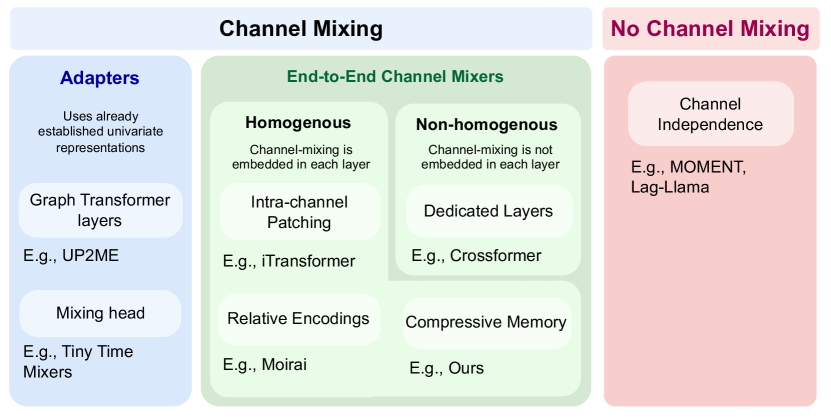
Channel Independence. Many multivariate time series models [15], including foundation models [8, 19, 4, 1], treat different channels independently. These approaches are simple, scalable, and typically perform well on real-world data and academic benchmarks [24] without substantial intra-channel dependencies.

To capture informative intra-channel dependencies in real-world time series, various channel-mixing approaches have been proposed in the literature:

Adapters. Approaches in this family usually first learn representations for each channel using a univariate backbone and then combine them using a multi-channel adapter. Examples include multivariate decoders [6] and Graph Transformer layers [23].

End-to-End Channel Mixers. These approaches tightly integrate channel mixing throughout the architecture. For instance, MOIRAI [21] flattens channels and uses relative channel encodings to distinguish information from different channels. iTransformer [13] attends to the inverted “variate“ tokens which capture multi-variate correlations. In each of these approaches, every layer of the model is homogeneous and performs the same computation. Other methods such as Crossformer [22] are non-homogeneous as they use different attention matrices to model inter-sequence and intra-channel information. Our proposed Infini-Channel Mixer method attaches compressive memory to each Transformer layer and is therefore a homogeneous end-to-end channel mixer by design.

4 Infini-Channel Mixer: Unlocking Multivariate Context using Compressive Memory

Figure 2: Infini-Channel Mixer (ICM) uses a learned scalar $\beta$, to balance local information from dot product attention with global information from the compressive memory matrix which aggregates cross-channel information.

Requirements. Our goal is to modify the standard transformer architecture minimally to accommodate multivariate time series. To simplify development and keep multivariate context expansion our primary focus, we fix the maximum length of time series that can be processed by our model. Given the prevalence of encoders in time series foundation models [8, 21, 1], the proposed architecture should be amenable to bidirectional self-attention.

Infini-Channel Mixer (ICM). To aggregate information from an arbitrary number of channels, we propose incorporating compressive memory into Transformers. Compressive memory systems use a fixed number of parameters to store and retrieve information efficiently. Our approach is inspired by Infini-attention [14], a recent compressive memory-based attention mechanism that has enabled decoder-only LLMs to, in theory, scale to infinitely long input sequences. Unlike Infini-attention, our approach uses memory to process multiple channels in transformers with encoders.

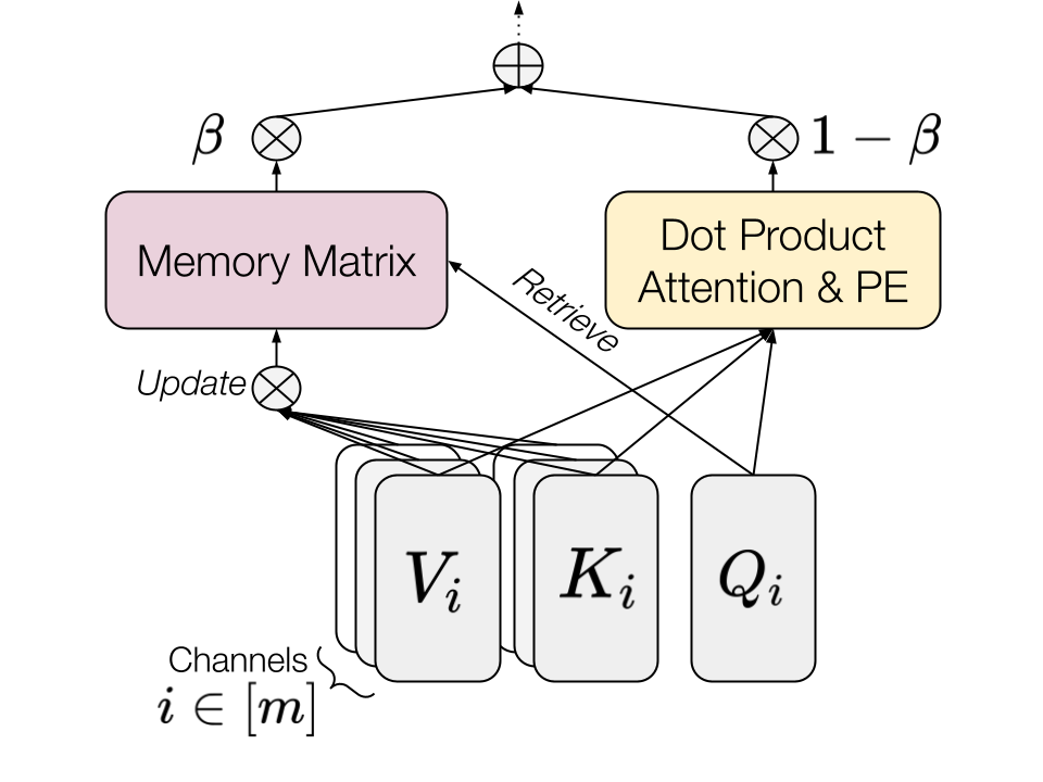
Infini-Channel Mixer extends a standard self-attention layer with a compressive memory matrix allowing it to attend to both local (intra-channel) and global (inter-channel) information. The memory matrix is computed by reusing the key ($\mathbf{K}$), query ($\mathbf{Q}$), and value ($\mathbf{V}$) matrices from the dot product attention as shown in Fig. 2, which accelerates training and inference and acts as a regularizer. A learned gating scalar $\beta$ regulates the trade-off between global information queried from the memory matrix and local information from the dot-product attention of a specific channel. This memory mechanism is replicated for each attention head and layer.

Step 1: Aggregate Cross-channel Information into Compressive Memory. The compressive memory matrix, $\mathbf{M}\in\mathbb{R}^{h\times d_{k}\times d_{k}}$, and the normalization term, $\mathbf{z}\in\mathbb{R}^{h\times d_{k}\times 1}$, are initially set to zero. Here, $h$ is the number of attention heads, and $d_{k}$ is the key dimension. We store information from each channel, $i\in[m]$, by reusing its local $\mathbf{KV}$ entries. To ensure training stability, we follow prior work, and set the normalization term to the sum of key entries from all channels [14, 10], and use element-wise (Exponential Linear Unit) ELU $+\ 1$ as a non-linear projection function $\sigma$. We define n as sequence length and $\mathbf{K}^{i}_{j}$ denotes the key entries of the $i^{\text{th}}$ channel and the $j^{\text{th}}$ input token.

$$\mathbf{M} \leftarrow\mathbf{M}+\sigma(\mathbf{K}^{i})^{\top}\mathbf{V}^{i}\hskip 20.0pt\mathbf{z} \leftarrow\mathbf{z}+\sum_{j}^{n}\mathbf{\sigma}(\mathbf{K}^{i}_{j})$$ (1)

Step 2: Conditioning on Inter-channel and Intra-Channel Information. We use the query matrix to retrieve the cross-channel information $\mathbf{A}_{\text{mem}^{i}}$ from the memory. This retrieved information is then combined with the local attention state $\mathbf{A}_{\text{dot}^{i}}$ using the learned gating scalar $\beta$. This design adds only a single trainable parameter per head to regulate the trade-off between local and global information.

$$\mathbf{A}_{\text{mem}^{i}}=\frac{\sigma(\mathbf{Q}^{i})\mathbf{M}}{\sigma(\mathbf{Q}^{i})\mathbf{z}+\epsilon}\hskip 20.0pt\mathbf{A}_{i}=sigmoid(\beta)\odot\mathbf{A}_{\text{mem}^{i}}+(1-sigmoid(\beta))\odot\mathbf{A}_{\text{dot}^{i}}$$ (2)

5 Experiments and Results

The goals of our experiments are twofold: (1) to systematically compare ICM against alternative context expansion techniques, and (2) to assess its impact on pre-training. To evaluate context expansion techniques outlined in Section 3, we conduct several small-scale supervised experiments focusing on the long-horizon forecasting task. Then to study the impact of ICM on pre-training, we pre-train the same model both with and without ICM and then evaluate the resulting models on two downstream tasks: long-horizon forecasting and multivariate classification.

Model / Example	Class	Design	Exchange	ETTh1	ETTh2	ETTm1	ETTm2	Weather
N-BEATS [16]	No Channel Mixing	Channel Independence	0.524	0.461	0.410	0.346	0.278	0.211
MOMENT-Tiny [8]			0.249	0.418	0.359	0.339	0.234	0.206
UP2ME [23]	Adapter	Graph Transformer	0.240	0.435	0.367	0.340	0.237	0.204
Crossformer [22]	Non-homogeneous End-to-End Mixer	Dedicated Intra- Channel Attention	0.559	0.571	0.654	0.390	0.515	0.227
iTransformer [13]	Homogeneous End-to-End Channel Mixer	Multivariate Patching	0.245	0.429	0.380	0.353	0.251	0.212
MOIRAI [21]		Concatentation $+$ Relative Encoding	0.243	0.426	0.357	0.340	0.249	0.216
ICM (Ours)		Compressive Memory	0.232	0.416	0.349	0.333	0.234	0.205

Table 1: Forecasting MSE of all models averaged over 3 different horizons $[96,192,384]$. The best models are shown in bold and the second best ones are underlined. In most cases, Infini-Channel Mixer (ICM) outperforms considered alternatives. Complete results in Table 4 (Appendix C).

Supervised Long-horizon Forecasting Experiments.

Due to variations in architectures and experimental setups, findings from prior work are inconclusive on how to best endow multivariate context to time series models. We address this by carefully implementing all context expansion techniques from Figure 1 on the same model architecture and experimental settings of long-horizon forecasting [24]. We use MOMENT, a recent open-source multi-task foundation model as the base architecture for all our experiments. To accelerate the process, we introduce a Tiny variant of it based on T5-Efficient-Tiny architecture [20]. All model variants take time series of length 256 as input (lookback window) and forecast the next 96, 192, and 384 time steps. As is common practice, models are trained and evaluated using Mean Squared Error (MSE). The exact details of model architecture, experimental settings, and hyper-parameters are outlined in Appendix B.

Results summarized in Table 1 show that our proposed approach outperforms alternative context expansion techniques on average in most cases.

Model name	Fine-tune $\beta$	Exchange	ETTh1	ETTh2	ETTm1	ETTm2	Weather
MOMENT-Tiny	$-$	0.250	0.437	0.343	0.333	0.230	0.222
+Infini-Channel Mixer	$\times$	0.249	0.439	0.336	0.332	0.230	0.219
	$\checkmark$	0.247	0.436	0.337	0.330	0.228	0.214

Table 2: Forecasting MSE averaged over 3 horizons $[96,192,384]$. MOMENT-Tiny with Infini-Channel Mixer outperforms its vanilla variant on all datasets. Additionally, fine-tuning the $\beta$ parameters along with the forecasting head most often results in improved performance.

	MOMENT-Tiny	+ ICM
Mean	0.625	0.632
Std.	0.254	0.268
Median	0.616	0.704
Wins/Ties/Losses	12/2/12	12/2/12

Table 3: Accuracy of MOMENT-Tiny with and without ICM across 26 UEA multivariate classification datasets. Complete results in Table LABEL:table:multivariate_classification. The addition of compressive memory does not substantially change multivariate classification accuracy, however it improves results on smaller datasets.

Pre-training Experiments.

We pre-train 2 variants on MOMENT-Tiny: one with Infini-Channel Mixer and one without it. Pre-training multivariate foundation models is challenging due to the scarcity of public benchmark multivariate datasets and the complexity of managing time series with varying numbers of channels. To address these issues, we pre-train our models for one epoch on the Time Series Pile [8], using a mix of univariate and multivariate datasets. To manage memory consumption during training, we fix the maximum number of channels ($=8$) per batch and sub-sample time series with more channels. Both models are trained with a maximum sequence length of 256 time steps.

We evaluate the pre-trained models on two downstream tasks: long-horizon forecasting and unsupervised representation learning for classification. For the forecasting task, we fine-tune a simple linear forecasting head on the representations learned by our models, while keeping all other model parameters frozen, except for those in the forecasting head and the $\beta$ coefficients. We use the same 6 datasets as in the previous experiment. For classification, following standard practice [8], we obtain representations of time series in a zero-shot setting (without access to labels) and use these representations to train a Support Vector Machine. For these experiments, we use the UCR/UEA classification repository [3] which comprises both univariate and multivariate datasets, frequently used to benchmark classification algorithms.

Tables 2 and 3 summarize forecasting and classification results, details in Appendix C.

Discussion.

Our experiments demonstrate the potential of the Infini-Channel Mixer as an effective context expansion mechanism. Despite adding only 16 new parameters (one for each of the 16 attention heads in MOMENT-Tiny), our approach consistently outperformed alternative methods on datasets with cross-channel dependencies. Interestingly, on some datasets like ETTm2 and Weather, treating channels independently yielded better performance than many multivariate methods. This finding suggests that current academic benchmarks might not fully capture the benefits of multivariate modeling. The promising performance of the UP2ME [23] approach, which models a subset of channels with substantial cross-correlation, supports this observation. Additionally, the substantial performance gains achieved by fine-tuning the $\beta$ coefficients further indicate that they function as a soft-gating mechanism, enabling the model to focus on the most informative cross-channel information.

6 Conclusion and Future Work

We introduced Infini-Channel Mixer (ICM) , a novel compressive memory mechanism that enables encoder-based TSFMs to effectively handle multivariate time series data. We systematically compared our proposed approach with multiple context expansion techniques proposed in the literature. We demonstrated that ICM, with only a few additional parameters, can improve the performance of time series models on two important tasks: long-horizon forecasting and classification. Future work should focus on rigorously evaluating our approach on larger models, across a wider range of datasets and tasks. Additionally, there is a pressing need for more multivariate datasets with strong cross-channel dependencies to better pre-train and evaluate large-scale models. It will also be important to explore whether Infini-Channel Mixer can be effectively adapted to handle extremely long time series.

Appendix A Channel Mixing

A.1 Concatenation Approach

In order to perform information exchange between the multiple variates, they have to be processed either at the same time, producing a higher memory cost, or sequentially, producing a higher computational cost. The default way of processing multiple variates is related to flattening the data from all channels, concatenating it, and producing an attention matrix with two dimensions equal to (channel number $\times$ sequence length). Woo et al. [21] implements a similar approach with inter- and intra-channel bias scalars, akin to the concept of relative positional biases in Raffel et al. [18]. The approach of concatenating [21] all of the variates is expressed in 3. To be able to ablate the approach, we do not apply the proposed rotary positional encoding, we stick to the sinusoidal position encoding.

$$E_{ij,mn}=\left(\mathbf{x}_{i,m}\mathbf{W}^{Q}\right)\left(\mathbf{x}_{j,n}\mathbf{W}^{K}\right)^{\top}+\delta_{mn}\cdot u^{(1)}+(1-\delta_{mn})\cdot u^{(2)}$$ (3)

where:

• $\mathbf{x}_{i,m}$ and $\mathbf{x}_{j,n}$ are the input vectors for tokens $i$ and $j$ of variates $m$ and $n$, respectively.

• $\mathbf{W}^{Q}$ and $\mathbf{W}^{K}$ are the weight matrices for queries and keys.

• $u^{(1)}$ and $u^{(2)}$ are scalar bias terms. $u^{(1)}$ is added when $m=n$, and $u^{(2)}$ is added when $m\neq n$.

• $\delta_{mn}$ is the Kronecker delta function, which is 1 if $m=n$ and 0 otherwise.

• $E_{ij,mn}$ represents the attention score between tokens $i$ and $j$ of variates $m$ and $n$, respectively.

A.2 Infini-Channel Mixer + Static

We would like to point out, that the novel concept of a memory matrix opens up possibilities to query a matrix differently, based on the inter-channel relations. A simple, but naive way of ensuring that is to add channel embeddings to each patch embedding in the embedding layer.

Let $\mathbf{E}_{\text{channel}}\in\mathbb{R}^{\text{channel\_num}\times d_{\text{model}}}$ be the matrix of static channel embeddings, where each row represents a unique embedding for a channel. The channel embeddings are broadcasted to match the dimensions of the input tensor and added to the patch embeddings. This operation can be mathematically represented as:

$$\mathbf{x}^{\prime}_{b,c,t,d}=\mathbf{x}_{b,c,t,d}+\mathbf{E}_{\text{channel},c,d}$$ (4)

where:

• $\mathbf{x}_{b,c,t,d}$ is the patched and embedded input

• $\mathbf{E}_{\text{channel},c,d}$ is the learned static channel embedding for the $c$-th channel and $d$-th dimension,

• $\mathbf{x}^{\prime}_{b,c,t,d}$ is the updated embedding after adding the channel embedding.

This method is denoted as "Infini-Channel Mixer + Static" in the supervised setting in the table 5

Appendix B Training Experimental Setup

B.1 Supervised Setting

In the supervised setting, we evaluate the following models using a consistent training setup:

• N-BEATS: For training N-BEATS, we use the following configuration: Stack Types (Trend and Seasonality), Number of Blocks per Stack (3), Theta Dimensions (4 and 8), and Hidden Layer Units (256). The training is conducted for 10 epochs with a batch size of 64, and is directly copied from Goswami et al. [8].

• Concatenation and Infini-Channel Mixer: For the Concatenation, Infini-Channel Mixer, and Infini-Channel Mixer + Static models, we employ the T5-Efficient-TINY backbone. This backbone comprises 4 encoder blocks, a model dimension of 256, 4 attention heads, and feed-forward dimensions of size 1024. Detailed specifications for the concatenation method are included in the appendix A.1.

• MT + Graph Transformer Layer: For the MT model with an added Graph Transformer layer, we use the MOMENT-Tiny backbone, incorporating a Graph Transformer layer as detailed in Zhang et al. [23].

• Crossformer: We use the original parameters of the Crossformer including patch size 12, 3 encoder block layers, the feed-forward dimension of 128, model dimension of 256, and 4 attention heads.

Appendix C Forecasting and classification task

Pre-training

We use the pre-trained models: MOMENT-Tiny, MOMENT-Tiny + Infini-Channel Mixer. Both are pre-trained for one epoch and with the same amount of data. We want to ensure a constant number of channels in a single batch (either 1 or 8), thus for multivariate datasets, we divide them into subdatasets of 8 channels. In case we end up with less than 8 channels in a subdataset, we oversample the remaining channels. This yields two types of batches - univariate and multivariate. We then use them in the pre-training.

C.1 Forecasting

Since MOMENT can handle multiple tasks, we test our approach on forecasting (supervised 5 and pre-trained 4) and classification tasks (multivariate and univariate pre-trained models). After pre-training the MOMENT-Tiny + Infini-Channel Mixer models, we fine-tune the linear head, as well as the $\beta$ parameters.

Model name	Horizon	Exchange		ETTh1		ETTh2		ETTm1		ETTm2		Weather
		MAE	MSE	MAE	MSE	MAE	MSE	MAE	MSE	MAE	MSE	MAE	MSE
Pre-trained MT + Infini-Channel Mixer (8 folds)	96	0.229	0.104	0.407	0.403	0.344	0.288	0.347	0.293	0.257	0.171	0.217	0.166
	192	0.326	0.207	0.427	0.438	0.388	0.351	0.367	0.327	0.295	0.224	0.252	0.207
	384	0.482	0.430	0.447	0.467	0.413	0.371	0.391	0.369	0.340	0.291	0.299	0.271
Pre-trained MT + Infini-Channel Mixer (4 folds)	96	0.227	0.102	0.407	0.399	0.348	0.292	0.348	0.291	0.259	0.171	0.216	0.164
	192	0.328	0.209	0.427	0.436	0.391	0.358	0.371	0.327	0.297	0.227	0.252	0.205
	384	0.482	0.432	0.445	0.464	0.415	0.374	0.395	0.367	0.345	0.297	0.298	0.268
Pre-trained Univariate MT	96	0.236	0.109	0.413	0.410	0.348	0.296	0.348	0.295	0.260	0.173	0.222	0.173
	192	0.338	0.217	0.432	0.442	0.390	0.359	0.369	0.331	0.296	0.226	0.258	0.217
	384	0.479	0.425	0.445	0.459	0.408	0.374	0.393	0.373	0.339	0.291	0.301	0.277

Table 4: MAE and MSE for various models across different datasets and horizons. The best metric for each dataset and horizon is highlighted, results better than MOMENT-Tiny are underlined. MT means MOMENT-Tiny as a backbone architecture, each model is pre-trained on ONE Epoch of the Time Series Pile.

Model name	Horizon	Exchange		ETTh1		ETTh2		ETTm1		ETTm2		Weather
		MAE	MSE	MAE	MSE	MAE	MSE	MAE	MSE	MAE	MSE	MAE	MSE
MT + Graph Transformer layer	96	0.210	0.089	0.409	0.382	0.365	0.316	0.349	0.304	0.256	0.170	0.197	0.151
	192	0.335	0.222	0.436	0.435	0.413	0.385	0.372	0.339	0.299	0.231	0.241	0.196
	384	0.470	0.409	0.477	0.489	0.429	0.399	0.397	0.376	0.354	0.310	0.292	0.264
NBeats	96	0.316	0.173	0.422	0.407	0.377	0.334	0.357	0.304	0.268	0.180	0.207	0.152
	192	0.527	0.467	0.456	0.453	0.422	0.392	0.379	0.339	0.320	0.266	0.273	0.208
	384	0.739	0.933	0.500	0.523	0.500	0.503	0.413	0.394	0.394	0.389	0.323	0.273
CrossFormer	96	0.385	0.260	0.448	0.427	0.540	0.575	0.365	0.317	0.383	0.312	0.218	0.148
	192	0.606	0.644	0.508	0.515	0.573	0.640	0.380	0.353	0.589	0.632	0.281	0.204
	384	0.704	0.774	0.668	0.770	0.644	0.746	0.507	0.501	0.573	0.601	0.378	0.329
iTransformer	96	0.231	0.104	0.408	0.391	0.373	0.325	0.361	0.311	0.268	0.186	0.207	0.160
	192	0.332	0.208	0.434	0.434	0.417	0.400	0.383	0.350	0.315	0.258	0.250	0.206
	384	0.480	0.423	0.452	0.462	0.434	0.414	0.409	0.397	0.353	0.310	0.299	0.272
Infini-Channel Mixer MT (Ours)	96	0.219	0.096	0.400	0.383	0.346	0.295	0.348	0.298	0.255	0.170	0.203	0.154
	192	0.316	0.193	0.421	0.420	0.396	0.368	0.369	0.330	0.296	0.229	0.244	0.197
	384	0.467	0.407	0.440	0.446	0.417	0.385	0.394	0.372	0.345	0.304	0.295	0.263
Infini-Channel Mixer + Static MT (Ours)	96	0.224	0.100	0.405	0.390	0.354	0.300	0.346	0.298	0.252	0.167	0.201	0.148
	192	0.322	0.204	0.428	0.427	0.398	0.362	0.369	0.330	0.294	0.224	0.244	0.192
	384	0.483	0.437	0.441	0.448	0.438	0.409	0.395	0.373	0.346	0.303	0.293	0.258
Channel Concatenation	96	0.223	0.099	0.410	0.393	0.356	0.303	0.353	0.302	0.264	0.180	0.211	0.166
	192	0.329	0.213	0.430	0.429	0.396	0.370	0.377	0.339	0.305	0.238	0.251	0.210
	384	0.478	0.418	0.448	0.456	0.428	0.399	0.400	0.380	0.364	0.329	0.297	0.273
Univariate MT	96	0.204	0.084	0.407	0.388	0.354	0.300	0.351	0.300	0.254	0.167	0.201	0.155
	192	0.323	0.202	0.425	0.422	0.399	0.376	0.374	0.338	0.303	0.235	0.242	0.198
	384	0.499	0.460	0.442	0.445	0.420	0.399	0.399	0.379	0.344	0.301	0.292	0.264

Table 5: MAE and MSE for various models, forecasting, supervised setup, across different datasets and horizons. The best metric for each dataset and horizon is highlighted, results better than MOMENT-Tiny are underlined. MT means MOMENT-Tiny as a backbone architecture. Our method shows promising results, with notably the moment backbone paired with the Graph Transformer layer showing good results on the Weather dataset.

C.2 Classification

In the multivariate case, MOMENT-Tiny + Infini-Channel Mixer achieves comparable results to MOMENT-Tiny 3, although mean and median accuracy is higher, the number of wins/losses for MOMENT-Tiny + Infini-Channel Mixer is 9155 / 6512, which is worse than for MOMENT-Tiny 9497 / 6170. We hypothesize that this happens because the $\beta$ parameters allow the model backbone to adjust during the fine-tuning stage. In the univariate case, our model with Channel-Mixing performs worse than the vanilla one. This points towards the hypothesis that meaningful filtering of the aggregated memory is an important direction of future work. LABEL:table:multivariate_classification LABEL:table:univariate_classification.

Table 6: Accuracy for multivariate datasets (UCR/UEA) classification for MOMENT-Tiny and MOMENT-Tiny + Infini-Channel Mixing.

Dataset	MOMENT-Tiny	MOMENT-Tiny + Infini-Channel Mixing Mixer
ArticularyWordRecognition	0.923	0.943
AtrialFibrillation	0.400	0.333
BasicMotions	0.550	0.875
Cricket	0.972	0.972
DuckDuckGeese	0.540	0.340
EigenWorms	0.557	0.542
Epilepsy	0.949	0.971
ERing	0.852	0.811
EthanolConcentration	0.346	0.281
FingerMovements	0.500	0.650
HandMovementDirection	0.230	0.284
Handwriting	0.212	0.179
Heartbeat	0.722	0.722
JapaneseVowels	0.676	0.692
Libras	0.850	0.822
LSST	0.329	0.266
MotorImagery	0.480	0.520
NATOPS	0.772	0.828
PEMS-SF	0.879	0.855
PenDigits	0.959	0.971
PhonemeSpectra	0.212	0.175
RacketSports	0.697	0.717
SelfRegulationSCP1	0.785	0.724
SelfRegulationSCP2	0.489	0.550
SpokenArabicDigits	0.966	0.928
StandWalkJump	0.400	0.467

Table 7: Accuracy for univariate datasets (UCR/UEA) classification for MOMENT-Tiny and MOMENTiTiny + Infini-Channel Mixing

Dataset	MOMENT-Tiny	MOMENT-Tiny + Infini-Channel Mixing
GestureMidAirD2	0.538	0.515
UWaveGestureLibraryX	0.790	0.745
GesturePebbleZ2	0.791	0.722
ECG5000	0.921	0.934
OSULeaf	0.802	0.719
MedicalImages	0.759	0.658
Ham	0.543	0.581
DistalPhalanxTW	0.612	0.619
ProximalPhalanxOutlineCorrect	0.842	0.838
FreezerRegularTrain	0.961	0.946
TwoLeadECG	0.748	0.838
GunPointMaleVersusFemale	0.975	0.984
Trace	0.980	0.940
SmoothSubspace	0.793	0.867
MiddlePhalanxTW	0.558	0.552
SyntheticControl	0.950	0.880
ShapesAll	0.772	0.725
AllGestureWiimoteX	0.627	0.520
Wafer	0.996	0.994
FaceFour	0.557	0.443
CricketX	0.641	0.541
DistalPhalanxOutlineCorrect	0.714	0.707
ChlorineConcentration	0.671	0.702
Chinatown	0.980	0.971
GestureMidAirD1	0.623	0.523
MiddlePhalanxOutlineAgeGroup	0.526	0.468
UMD	0.965	0.917
Crop	0.701	0.701
GesturePebbleZ1	0.901	0.797
WordSynonyms	0.577	0.475
ArrowHead	0.571	0.520
Wine	0.556	0.500
Coffee	0.821	0.536
Earthquakes	0.748	0.748
Herring	0.594	0.594
Beef	0.667	0.700
MiddlePhalanxOutlineCorrect	0.526	0.591
ECGFiveDays	0.844	0.742
Yoga	0.742	0.751
Adiac	0.627	0.619
MoteStrain	0.654	0.712
Strawberry	0.922	0.924
InsectWingbeatSound	0.563	0.508
DodgerLoopWeekend	0.848	0.703
Meat	0.833	0.833
MelbournePedestrian	0.870	0.872
FaceAll	0.666	0.615
FacesUCR	0.652	0.606
AllGestureWiimoteY	0.671	0.589
ShakeGestureWiimoteZ	0.760	0.720
BME	0.947	0.960
FordB	0.810	0.786
Fish	0.777	0.629
SonyAIBORobotSurface2	0.821	0.753
FiftyWords	0.677	0.589
ToeSegmentation1	0.925	0.851
FreezerSmallTrain	0.744	0.747
TwoPatterns	0.964	0.821
ShapeletSim	0.650	0.594
Plane	0.952	0.933
GestureMidAirD3	0.315	0.292
DiatomSizeReduction	0.784	0.765
CricketZ	0.669	0.564
Lightning7	0.589	0.548
UWaveGestureLibraryY	0.723	0.633
GunPointAgeSpan	0.949	0.965
DistalPhalanxOutlineAgeGroup	0.683	0.676
SwedishLeaf	0.875	0.840
CBF	0.864	0.671
BeetleFly	0.750	0.650
AllGestureWiimoteZ	0.569	0.466
DodgerLoopDay	0.400	0.263
GunPointOldVersusYoung	0.933	0.889
FordA	0.934	0.913
ItalyPowerDemand	0.935	0.900
ProximalPhalanxOutlineAgeGroup	0.839	0.829
GunPoint	0.960	0.940
ProximalPhalanxTW	0.737	0.732
PickupGestureWiimoteZ	0.640	0.480
SonyAIBORobotSurface1	0.626	0.687
PowerCons	0.894	0.833
PhalangesOutlinesCorrect	0.699	0.650
BirdChicken	0.900	0.750
ToeSegmentation2	0.938	0.869
CricketY	0.585	0.482
ElectricDevices	0.634	0.638
DodgerLoopGame	0.623	0.551
Fungi	0.887	0.806
Symbols	0.857	0.842
UWaveGestureLibraryZ	0.750	0.678
ECG200	0.840	0.840

References

- Ansari et al. [2024] Abdul Fatir Ansari, Lorenzo Stella, Caner Turkmen, Xiyuan Zhang, Pedro Mercado, Huibin Shen, Oleksandr Shchur, Syama Syndar Rangapuram, Sebastian Pineda Arango, Shubham Kapoor, Jasper Zschiegner, Danielle C. Maddix, Hao Wang, Michael W. Mahoney, Kari Torkkola, Andrew Gordon Wilson, Michael Bohlke-Schneider, and Yuyang Wang. Chronos: Learning the language of time series. arXiv preprint arXiv:2403.07815, 2024.
- Brown et al. [2020] Tom B Brown, Benjamin Mann, Nick Ryder, et al. Language models are few-shot learners. arXiv preprint arXiv:2005.14165, 2020.
- Chen et al. [2015] Yanping Chen, Eamonn Keogh, Bing Hu, Nurjahan Begum, Anthony Bagnall, Abdullah Mueen, and Gustavo Batista. The UCR time series classification archive, July 2015. www.cs.ucr.edu/~eamonn/time_series_data/.
- Das et al. [2023] Abhimanyu Das, Weihao Kong, Rajat Sen, and Yichen Zhou. A decoder-only foundation model for time-series forecasting. arXiv preprint arXiv:2310.10688, 2023.
- Devlin et al. [2018] Jacob Devlin, Ming-Wei Chang, Kenton Lee, and Kristina Toutanova. BERT: Pre-training of deep bidirectional transformers for language understanding. arXiv preprint arXiv:1810.04805, 2018.
- Ekambaram et al. [2024] Vijay Ekambaram, Arindam Jati, Nam H Nguyen, Pankaj Dayama, Chandra Reddy, Wesley M Gifford, and Jayant Kalagnanam. TTMs: Fast multi-level tiny time mixers for improved zero-shot and few-shot forecasting of multivariate time series. arXiv preprint arXiv:2401.03955, 2024.
- Garza and Mergenthaler-Canseco [2023] Azul Garza and Max Mergenthaler-Canseco. TimeGPT-1, 2023.
- Goswami et al. [2024] Mononito Goswami, Konrad Szafer, Arjun Choudhry, Yifu Cai, Shuo Li, and Artur Dubrawski. MOMENT: A family of open time-series foundation models. In International Conference on Machine Learning, 2024.
- Jin et al. [2023] Ming Jin, Shuang Wang, Li Ma, Zhen Chu, Jia-Yu Zhang, Xiong Shi, Pei-Yuan Chen, Yanzhi Liang, Yufeng Li, Sinno Pan, and Qian Wen. Time-LLM: Time series forecasting by reprogramming large language models. arXiv preprint arXiv:2310.01728, 2023.
- Katharopoulos et al. [2020] Angelos Katharopoulos, Apoorv Vyas, Nikolaos Pappas, and François Fleuret. Transformers are RNNs: Fast autoregressive transformers with linear attention. In Hal Daumé III and Aarti Singh, editors, Proceedings of the 37th International Conference on Machine Learning, volume 119 of Proceedings of Machine Learning Research, pages 5156–5165. PMLR, 13–18 Jul 2020. URL https://proceedings.mlr.press/v119/katharopoulos20a.html.
- Liu et al. [2019] Yinhan Liu, Myle Ott, Naman Goyal, et al. RoBERTa: A robustly optimized BERT pretraining approach. arXiv preprint arXiv:1907.11692, 2019.
- [12] Yong Liu, Haoran Zhang, Chenyu Li, Xiangdong Huang, Jianmin Wang, and Mingsheng Long. Timer: Generative pre-trained transformers are large time series models. In Forty-first International Conference on Machine Learning.
- Liu et al. [2024] Yong Liu, Tengge Hu, Haoran Zhang, Haixu Wu, Shiyu Wang, Lintao Ma, and Mingsheng Long. iTransformer: Inverted transformers are effective for time series forecasting. In The Twelfth International Conference on Learning Representations, 2024. URL https://openreview.net/forum?id=JePfAI8fah.
- Munkhdalai et al. [2024] Tsendsuren Munkhdalai, Manaal Faruqui, and Siddharth Gopal. Leave no context behind: Efficient infinite context transformers with infini-attention. arXiv preprint arXiv:2404.07143, 2024.
- Nie et al. [2023] Yuqi Nie, Nam H. Nguyen, Phanwadee Sinthong, and Jayant Kalagnanam. A time series is worth 64 words: Long-term forecasting with transformers. arXiv preprint arXiv:2307.13787, 2023. URL https://arxiv.org/abs/2307.13787.
- Oreshkin et al. [2019] Boris N. Oreshkin, Dmitri Carpov, Nicolas Chapados, and Yoshua Bengio. N-BEATS: neural basis expansion analysis for interpretable time series forecasting. CoRR, abs/1905.10437, 2019. URL http://arxiv.org/abs/1905.10437.
- Radford et al. [2019] Alec Radford, Jeffrey Wu, Rewon Child, David Luan, Dario Amodei, Ilya Sutskever, et al. Language models are unsupervised multitask learners. OpenAI blog, 1(8):9, 2019.
- Raffel et al. [2020] Colin Raffel, Noam Shazeer, Adam Roberts, Katherine Lee, Sharan Narang, Michael Matena, Yanqi Zhou, Wei Li, and Peter J. Liu. Exploring the limits of transfer learning with a Unified Text-to-Text Transformer. Journal of Machine Learning Research, 21(140):1–67, 2020. URL http://jmlr.org/papers/v21/20-074.html.
- Rasul et al. [2023] Kashif Rasul, Arjun Ashok, Andrew Robert Williams, Arian Khorasani, George Adamopoulos, Rishika Bhagwatkar, Marin Biloš, Hena Ghonia, Nadhir Vincent Hassen, Anderson Schneider, et al. Lag-Llama: Towards foundation models for probabilistic time series forecasting. arXiv preprint arXiv:2310.08278, 2023.
- Tay et al. [2022] Yi Tay, Mostafa Dehghani, Jinfeng Rao, William Fedus, Samira Abnar, Hyung Won Chung, Sharan Narang, Dani Yogatama, Ashish Vaswani, and Donald Metzler. Scale efficiently: Insights from pre-training and fine-tuning transformers, 2022. URL https://arxiv.org/abs/2109.10686.
- Woo et al. [2024] Gerald Woo, Chenghao Liu, Akshat Kumar, Caiming Xiong, Silvio Savarese, and Doyen Sahoo. Unified training of universal time series forecasting transformers. In Proceedings of the 41st International Conference on Machine Learning, Vienna, Austria, 2024. International Conference on Machine Learning.
- Zhang and Yan [2023] Yunhao Zhang and Junchi Yan. Crossformer: Transformer utilizing cross-dimension dependency for multivariate time series forecasting. In The Eleventh International Conference on Learning Representations, 2023.
- Zhang et al. [2024] Yunhao Zhang, Minghao Liu, Shengyang Zhou, and Junchi Yan. UP2ME: Univariate pre-training to multivariate fine-tuning as a general-purpose framework for multivariate time series analysis. In Forty-first International Conference on Machine Learning, 2024.
- Zhou et al. [2021] Haixu Zhou, Shanghang Zhang, Jie Peng, Shuai Zhang, Guangjian Li, Hanzhang Xiong, Wancai Zhang, Tien-Ju Lin, Xiaolong Chu, Jingren Zhang, et al. Informer: Beyond efficient transformer for long sequence time-series forecasting. In Proceedings of the AAAI Conference on Artificial Intelligence, 2021.