Fast Streaming Transducer ASR Prototyping via
Knowledge Distillation with Whisper

Abstract

The training of automatic speech recognition (ASR) with little to no supervised data remains an open question. In this work, we demonstrate that streaming Transformer-Transducer (TT) models can be trained from scratch in consumer and accessible GPUs in their entirety with pseudo-labeled (PL) speech from foundational speech models (FSM). This allows training a robust ASR model just in one stage and does not require large data and computational budget compared to the two-step scenario with pre-training and fine-tuning. We perform a comprehensive ablation on different aspects of PL-based streaming TT models such as the impact of (1) shallow fusion of n-gram LMs, (2) contextual biasing with named entities, (3) chunk-wise decoding for low-latency streaming applications, and (4) TT overall performance as the function of the FSM size. Our results demonstrate that TT can be trained from scratch without supervised data, even with very noisy PLs. We validate the proposed framework on 6 languages from CommonVoice and propose multiple heuristics to filter out hallucinated PLs.

Fast Streaming Transducer ASR Prototyping via
Knowledge Distillation with Whisper

Iuliia Thorbecke^1,2 Juan Zuluaga-Gomez^1,3 Esaú Villatoro-Tello¹ Shashi Kumar^1,3 Pradeep Rangappa¹ Sergio Burdisso¹ Petr Motlicek^1,4 Karthik Pandia⁵ Aravind Ganapathiraju^{5 1} Idiap Research Institute ² University of Zurich ³ EPFL ⁴ Brno University of Technology ⁵ Uniphore iuliia.thorbecke@uzh.ch juan.zuluaga@eu4m.eu

1 Introduction

There are many challenges when developing automatic speech recognition (ASR) engines for industrial applications, including (1) large-scale databases that generalize across multiple domains; (2) inference under challenging low-latency settings; and (3) lightweight ASR model size to minimize deployment costs. While the first has been solved by training large acoustic foundational speech models (FSM) with massive databases (Conneau et al., 2020; Pratap et al., 2023), the latter two strongly relate to architectural choices, e.g., using Connectionist Temporal Classification (CTC) (Graves et al., 2006) or transducer-based (Graves, 2012) modeling.

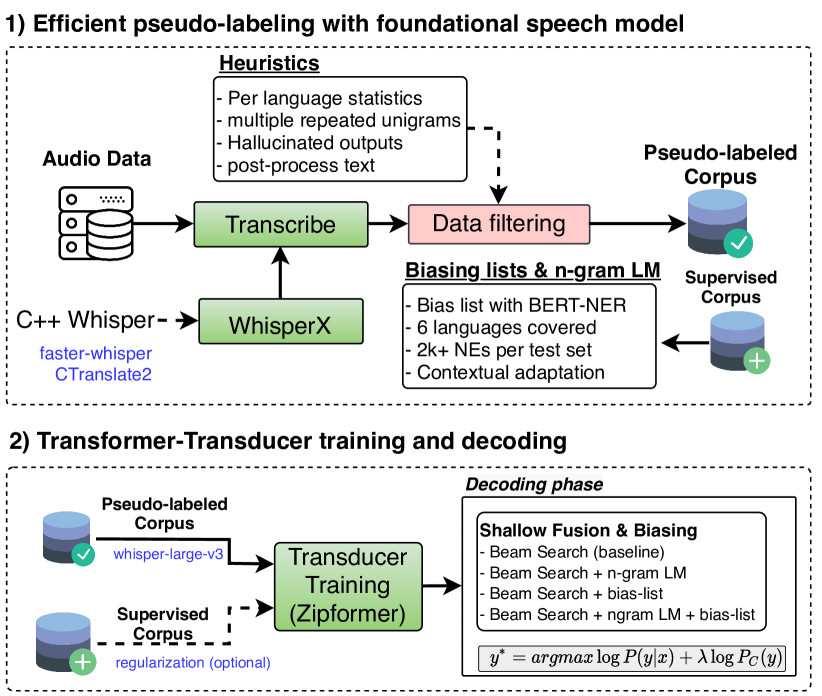
Figure 1: Proposed framework for efficient and fast streaming ASR prototyping with pseudo-labeled data. Transducer model are further improved via shallow fusion of n-gram LMs and contextual biasing of target named entities.

In industrial applications, large supervised databases in target domains are not always available, thus several techniques have been proposed to develop robust ASR models with small supervised corpora: (1) data augmentation (Park et al., 2019; Bartelds et al., 2023); (2) only-audio self-supervised pre-training with large databases and fine-tuning with small corpora (Baevski et al., 2020; Conneau et al., 2020; Zuluaga-Gomez et al., 2023); (3) pseudo-label then fine-tune, e.g., semi-supervised learning (Zhu et al., 2023; Lugosch et al., 2022; Zuluaga-Gomez et al., 2021) and weakly supervised learning  (Radford et al., 2022). Most of the approaches target the attention-based encoder-decoder (AED) (Watanabe et al., 2017a) or CTC models. Even though these two architectures have shown impressive results on multiple benchmarks (e.g., Whisper (Radford et al., 2022)), they still lag in streaming settings (Prabhavalkar et al., 2023).

The Transformer-Transducer architecture (Yeh et al., 2019) is widely exploited for industrial uses that require streaming decoding because the transducer decoder naturally supports streaming (Li et al., 2021, 2020). However, the transducer used to be harder to train compared to AED and CTC, thus, it was less explored in the community, until it was shown to achieve a performance as close as AED models (Sainath et al., 2020). The transducer models consist of an encoder, predictor and joint networks. Using a Transformer (Vaswani et al., 2017) encoder leads to a Transformer-Transducer (TT) architecture (Battenberg et al., 2017; Yeh et al., 2019; Zhang et al., 2020). When trained from scratch, the TT models require sufficient amounts of supervised datasets in the target language and domain (Noroozi et al., 2023; Li et al., 2021). At the same time, fine-tuning a large pre-trained model, even when using a transducer decoder, would not allow streaming decoding.

In this work, we focus on two questions partly unanswered by the research community: (1) Could we quickly prototype a streaming TT model on a single accessible GPU? (2) Can we train TT models with only pseudo-labeled (PL) data? We target the streaming scenario, which is by nature more challenging than standard offline (full attention) decoding (Sainath et al., 2020). Despite the robustness of AED models in the offline scenario, they still require a large amount of supervised data. Here, we use TT models (Yeh et al., 2019), where the challenge arises on the fact that these do not include a self-supervised stage, i.e., needing audio-text pairs always. We demonstrate that TT models can be trained entirely from scratch with PLs generated from Whisper (Radford et al., 2022) while attaining competitive performance in streaming scenarios. The overall proposed approach is illustrated in Figure 1.

Contributions:

• We propose a framework for full-stack rapid development of ASR streaming solutions from scratch with low-to-zero supervised resources;

• comprehensive study of TT performance as a function of the pseudo-labels quality, for both, online and offline settings;

• robust heuristics to filter out noisy and hallucinated PLs from FSM;

• evaluation of the impact of shallow fusion with external n-gram LM and contextual biasing for named entities;

• experimentation and validation on 6 languages from CommonVoice.

2 Related Work

Developing robust ASR systems for low-latency online settings with little to no supervised data is still an open challenge in the community. In this section, we introduce the most prominent approaches to overcome these issues.

From Encoder-Decoder to Transducer models

One of the key advantages of transducer models over encoder-decoder relies on the fact that it supports streaming decoding. Not until recently, it has been demonstrated that these models can surpass standard AED systems  (Sainath et al., 2020). There have been multiple breakthroughs that have made transducer training easier, such as (1) pruned transducer loss  (Kuang et al., 2022), (2) better architectures, e.g., FastConformer (Rekesh et al., 2023); and (3) from the modeling side, e.g., model pruning, sparsification (Yang et al., 2022a), and quantization (Sainath et al., 2020). However, little to no work has been done on fast TT model prototyping (few GPU-days) with pure pseudo-labeled data.

Pseudo-labeling in ASR

Semi-supervised learning (Higuchi et al., 2021), pseudo labeling (Zavaliagkos and Colthurst, 1998), and weakly supervised learning (Radford et al., 2022) are a family of methods aiming to partly alleviate the burden of lack of labeled data for supervised ASR training. These approaches have shown promising word error rate (WER) improvement in multiple settings and languages. In practice, a teacher model $g$ is trained on an audio-text paired corpus $D_{l}=\{X_{i},Y_{i}\}$. Then, it is used to pseudo label a much larger unlabeled only audio corpus, $D_{pl}=\{X_{i},Y^{*}_{i}\}$. Afterward, usually a smaller model (Barrault et al., 2023) can use $D_{l}$ and $D_{pl}$ for supervised training or fine-tuning (Hsu et al., 2021). However, PLs are often noisy and bounded by $g$ model quality, whereas their use might result in suboptimal final performance in the models. This can be solved by either filtering out the nosiest samples or increasing $g$ model size to improve their quality. Several approaches to improve the PL quality include improving loss functions (Zhu et al., 2023; Gao et al., 2023), pairing online and offline models at training time (Higuchi et al., 2021), and continuous single-language  (Likhomanenko et al., 2022; Berrebbi et al., 2022) and multilingual pseudo-labeling setting (Lugosch et al., 2022).

Knowledge Distillation with Large Models

Knowledge distillation (KD), or teacher-student training (Watanabe et al., 2017b), is a very well-known technique to distill knowledge from a large model into a smaller model (Hinton et al., 2015). The former is considered the Teacher and the latter is the Student. In this framework, we first train the teacher model with the correct label (e.g., supervised training) (Takashima et al., 2018) or in a self-supervised manner. The student model is then trained with the posterior distributions of the pre-trained teacher model (Chebotar and Waters, 2016). There has been prior work on KD for CTC (Takashima et al., 2018) and AED models with Whisper (Radford et al., 2022) (Gandhi et al., 2023; Ferraz et al., 2024) and Transducer models (Panchapagesan et al., 2021). Similarly, work to distil offline transducer models into online has been explored by Kurata and Saon (2020) or from self-supervised models (Yang et al., 2022b).

In our work, we focus on sequence-level KD, which means we use the one-best hypothesis from the teacher model instead of using the posterior distribution. This approach has some benefits: (1) no need to cache the teacher model or its outputs into memory; (2) no need to modify the current ASR training pipelines; (3) overall faster ASR training w.r.t teacher-student based KD, where we can leverage highly optimized inference pipelines–including model quantization–for PL generation, e.g., WhisperX (Bain et al., 2023). All this results in pseudo-labeling that meets the needs for fast prototyping for standard industrial applications.

3 Experimental Setup

This section describes the datasets, TT architecture, details for training with pseudo-labeled data, effective integration of language model and contextual biasing with shallow fusion, and metrics we use for evaluation.

3.1 Pseudo Labeling with Whisper

Our core contribution is the fast prototyping of TT streaming ASR trained exclusively on pseudo-labeled data. We select the Whisper model as our teacher model (Radford et al., 2022) due to its strong performance across multiple benchmarks. In addition, Whisper provides models at different parameter scales.

Decoding with WhisperX pipeline

We use the WhisperX pipeline (Bain et al., 2023) across all the experiments to generate PLs. It is composed of (1) a voice activity detection step to segment long-form audio; (2) batching multiple segments for efficient inference; (3) model quantization of Whisper and C++ implementation on FasterWhisper which uses CTranslate2 for fast decoding; (4) model inference and word level alignment. Note that we pseudo-label each training corpus with 5 Whisper model sizes, i.e., whisper-tiny, base, small, medium, and large-v3.

Data filtering heuristics

We developed multiple data selection heuristics ($H$) to filter out noisy and hallucinated PLs. $H1$: remove PL if composed of the same unigram three or more times. $H2$: compute maximum word length from supervised training corpus and remove utterances with one or more PLs larger than the max threshold. $H3$: compute $word_{ratio}$ and filter out samples with $word_{ratio}$ less than 1 or more than 4. $H4$: verbalize all the numbers from the pseudo-labels, remove punctuation and normalize following the CommonVoice recipe in Lhotse (Żelasko et al., 2021). These heuristics are applied for every training corpora. Similar heuristics are proposed in (Barrault et al., 2023).

3.2 Transformer-Transducer Training

We train Transformer-Transducer models from scratch for each language and dataset. We use stateless predictor (Ghodsi et al., 2020) and Zipformer encoder model (Yao et al., 2023) with the latest Icefall Transducer recipe and its default training hyper-parameters. This includes ScaledAdam optimizer (Kingma and Ba, 2014), learning rate scheduler with a 500-step warmup phase (Vaswani et al., 2017) followed by a decay phase (each 7.5k steps and 3.5 epochs), as in Yao et al. (2023). The neural TT model is jointly optimized with an interpolation of simple and pruned RNN-T loss (Kuang et al., 2022; Graves, 2012) and CTC loss (Graves et al., 2006) ($\lambda=0.1$), according to:

$$\mathcal{L}=(1-\lambda)\cdot\mathcal{L}_{RNN\-T}+\lambda\cdot\mathcal{L}_{CTC}.$$ (1)

The peak learning rate is $lr=5.0e^{-2}$ and we train each TT for 30 epochs on a single RTX 3090 GPU with only PLs. Training takes between 1 and 2 days.

Regularization with supervised data

We perform experiments where along with PLs we mix in 100h of randomly selected supervised data from the train set $D_{l}$ during training. We compute mixing weights between $D_{l}$ and $D_{pl}$ so each training batch contains at least one sample from $D_{l}$. This is achieved with CutSet.Mux function from Lhotse (Żelasko et al., 2021). All the experiments that uses PL and supervised data are denoted with +sup. [100h], otherwise, the model is trained with PL only. As an ablation experiment, we also test the performance by scaling up supervised data to 200h and 400h when using the weakest FSM, i.e., whisper-tiny. This experiment aims to (1) compensate for very low-quality PLs, and (2) demonstrate that Whisper PLs (from the largest models) are of sufficient quality for transducer training without any supervised data.

Enabling streaming decoding with multi-chunk training

All the models proposed in this work can perform streaming decoding. This is achieved by performing chunk-wise multi-chunk training. During training, we use causal masking of different sizes to enable streaming decoding under different low-latency configurations (Swietojanski et al., 2023; Kumar et al., 2024). Specifically, we rely on two lists: chunk-size={640ms,1280ms,2560ms,full} and left-context-frames={64,128,256,full}. At training time, we randomly select the chunk size and the left context chunks for each batch. This enables the final model to work on a wide variety of streaming settings. At test time, we select 13 different decoding configurations ranging from 320 ms to 2560 ms chunks (see App. A).

3.3 Language Modeling and Contextual Biasing

Leveraging more text data and context information with language model and keywords integration can considerably improve ASR performance. Since in our set-up, we assume that we have zero (or very little) supervised data, using extra unpaired text data would not contradict the original constraints. At the same time, relying mainly on pseudo-labels, we see text knowledge integration as an opportunity to make our models more reliable and robust. The widely used method of LM integration during the decoding is shallow fusion (SF) (Aleksic et al., 2015; Kannan et al., 2018; Zhao et al., 2019; Jung et al., 2022). SF means log-linear interpolation of the score from the ASR model with an external separately optimized LM at each step of the beam search:

$$y^{\ast}=\operatorname*{argmax}\log P(y|x)+\lambda\log P_{LM}(y),$$ (2)

where $P_{LM}(y)$ is an external LM and $\lambda$ is a hyperparameter to control the impact of the LM on the overall model score.

To gain more possible improvement from the text information, we explore three options with the SF: (1) word-level n-gram LM, (2) named-entities, (3) combination of word-level n-gram LM and named-entities. We choose n-gram over neural network (NN) LMs, as the use of NN-LMs would be impractical in low-latency streaming scenarios due to the size of the models. Named entities are extracted automatically and considered as keywords forming biasing lists: for more details see Section 3.4.1.

Shallow fusion with Aho-Corasick

One of the drawbacks of LM fusion is that it typically slows down the decoding time during inference, especially when using bigger NN-LMs. Since we focus on streaming ASR models in this paper, any potential increase in inference time is critical for us. Recent studies demonstrated that SF implemented with the Aho-Corasick (AC) algorithm (Aho and Corasick, 1975) is fast and optimized when used for the keyword biasing (Guo et al., 2023). Thus, we use the AC implementation from Icefall to integrate key named entities (NE) and word-level n-gram LMs during the decoding.

The Transducer model we use outputs its hypotheses at the subword level and, in this case, an external LM is also typically trained on subwords. In our experiments, to benefit from the word-level statistics, we integrate word-based n-gram external LMs. Such integration from word to subword level is possible with the AC implementation. First, the LM n-grams are converted into strings of subword units with SentecePieces; second, the subword units are used to build an AC prefix trie including LM weights in the probability domain.

When a string match occurs between a model prediction and a string in the prefix trie, the log probability of the matching hypothesis is augmented by the LM weight. To obtain positive cost, we convert the logarithmic LM weights (e.g., from ARPA) back to probabilities by taking an exponent. In the case of context biasing, SF works in the same way but instead of LM weights a fixed bias cost is added to each matched arc. Typically when applying context biasing alone, we set such cost to 0.7. For SF with combined n-gram LM and biasing list, we still use LM weights, bias cost, and a single prefix tree. Using a single prefix tree has the advantage of faster running time, which is relevant for streaming models. We tune the biasing cost on the dev sets and set it differently when a biased entity is present in the LM vs when it is not:

$$C=\begin{cases}\alpha_{outLM}&\text{if NE is not in LM,}\\ exp(LMw)+\alpha_{inLM}&\text{if NE is in LM,}\\ exp(LMw)&\text{otherwise.}\end{cases}$$

Language modeling

For LM SF, we train tri-gram word-level LMs with SRILM (Stolcke, 2002). To train n-gram LMs, we use text data from the corresponding train sets. All the train texts are uppercased and normalized to contain only unicode characters.

Evaluation protocol  For evaluation, we use the standard word error rate (WER) metric for ASR which is the lower the better.

3.4 Databases

Here, we introduce the datasets used for fast ASR prototyping and describe the process of generating biasing lists for each language.

3.4.1 CommonVoice Database

The CommonVoice dataset comprises several thousand hours of audio in more than 100 languages (Ardila et al., 2020). For experimentation, we select six languages from CommonVoice-v11 (Ardila et al., 2020) which have sufficient data for training ASR and language models: Catalan (CA), English (EN), German (DE), French (FR), Spanish (ES), and Italian (IT). We use the official train sets and report WERs on the official test sets. See Table 1 for further statistics.

Table 1: Train and test sets statistics with context information per CommonVoice language. ^†total of unique entities per test set after removing unigrams shorter than 5 characters. ^‡number of utterances in the test set with at least one named entity.

Lang	Train set	Test set stats & Named entities
(code)	[hr]	utt/hr	unique†	nb. utt‡
EN	1000	16K/27	6921	6442
CA	1200	16.3K/28	2108	2607
FR	600	16K/26	6035	7486
DE	600	16K/27	6949	8491
ES	317	15.5K/26	4776	6528
IT	200	15k/26	5838	5938

Biasing List Creation

We automatically create biasing lists for target CommonVoice subsets to perform the contextual biasing experiments. For this purpose, we use BERT models from HuggingFace (Wolf et al., 2020) fine-tuned on the named-entity recognition (NER) task for each language individually. The following steps are included: (1) automatic text labeling with BERT, (2) NEs extraction from the BERT labels, (3) NEs lists filtering. In Table 1, one can see the statistics of NE lists per language where the size of lists with unique NEs varies from 2108 to 6949 which is rather long for contextual biasing. The last column of Table 1 shows the number of utterances per test set that contain at least one NE. This information gives an estimation of the proportion of NEs in the test sets: DE and FR sets have almost half of the utterances with NEs, at the same time, the CA set has only 17% of those.

Heuristics for biasing list selection

Since NEs are automatically extracted with the BERT-based NER, extraction errors are inevitable. To minimize noise from potentially erroneously extracted NEs, we follow simple filtering heuristics when preparing the final biasing lists. $H1$: select only NEs that are composed of 1 to 4 words, and $H2$: remove single-word NEs shorter than 5 characters. For example, the filtering step is important to reduce such noisy outputs as short single words that often are not NEs: ich, wir, die – for DE, san, mar, new – for ES. We also tried to further filter the lists by only allowing NEs that are repeated at least twice, or NEs composed of bigram or more. However, in our experiments, only applying $H1$ and $H2$ was sufficient and yielded better WERs overall.

4 Results

We report our results in two parts. First, we present the overall performance of models trained with PL and with different settings. The following configurations are compared: (1) offline VS streaming TT models, (2)  models trained on PL-only VS models with supervised data regularization, and (3) models with different chunk sizes. Second, we report the performance of models with SF. For the baseline, we use a Zipformer streaming model trained per each language on PL only. In addition, we also compare our results to the offline Zipformer trained on the same data and include the reference to the previous results reported on CommonVoice in (Radford et al., 2022) (Table 3).

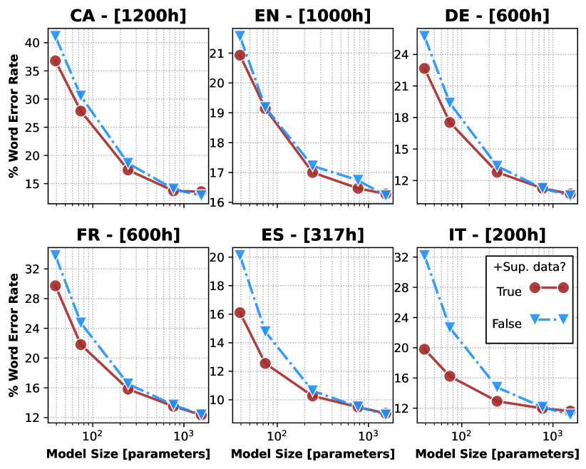
Figure 2: WERs for offline Zipformer models on six languages of CommonVoice. Models are trained with pseudo-labels from different Whisper model sizes (blue graphs). Adding 100h of supervised data during training (red graph) regularizes the training up to models with 700M params, especially for languages with less data.

4.1 Performance on models with PL of different quality

Offline models

In Figure 2, we present the offline results for TT models trained from scratch on PL data only in six languages (depicted by blue graphs). These models are evaluated only in a non-streaming context to determine the upper bound WERs achievable by training with PLs of varying qualities. As the size of the Whisper Model increases (shown on a log-scaled x-axis), there is a corresponding improvement in WERs, also on a log-scale. The best performance is observed for ES, with the least favourable results for EN. These results show that our approach adapts across a spectrum of PL data quantities and qualities, ranging from 200h for IT to over 1000h for CA and EN. We additionally analyzed the performance of models trained on PLs depending on how well each language is represented in the data used for training Whisper models (Radford et al., 2022). Yet, no consistent effect is noticed.

Regularization with supervised data

Red graphs in Figure 2 also show WERs for offline models that along with PLs include a small amount of supervised data, up to 100h, for regularization. This strategy proves to be beneficial in cases with noisier PLs, particularly for smaller Whisper models like Whisper-tiny, Whisper-base, and Whisper-small when WER goes down for all the languages. The benefits, however, decrease or are absent with more accurate PLs generated by larger models, such as Whisper-medium and Whisper-large-v3. Thus, with our results on six languages, we can conclude that when supervised data is available, regularization is recommended for models with weak PLs and can be omitted with strong PLs. The results with 100h regularization are also available in Table 3 for offline models and are consistent with the performance on streaming models reported in Table 2.

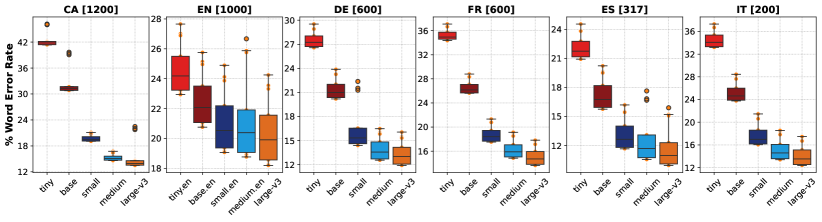
Figure 3: Box plots of WERs for six languages of CommonVoice. Streaming Zipformer models are trained from scratch, with only PLs generated with different Whisper model sizes. Each box denotes 13 decoding configurations, ranging from challenging (320ms chunk with limited left context) to more relaxed (2560ms chunk with full left context) streaming settings. (Note different WER scaling on the y-axis.)

Scaling-up supervised data helps on cases with very noisy PLs

For the ablation experiment on mixing in more supervised data, we maintain a fixed computational budget for generating PLs and explore the extent to which supervised data can offset noisy PLs. The results are pictured in Figure 4. Using only Whisper-tiny, we train TT models from scratch for the six CommonVoice languages with over 200h of available supervised data. Our results show significant improvements in WER as supervised data increases from 100h to 200h and even more so up to 400h, especially in languages like Catalan, French, and Italian, which likely suffer from lower-quality PLs. For this experiment, our oracle results are from the models fully trained on the supervised data, which can be found in Table 3 for offline models and in Table 2 for streaming models.

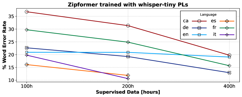
Figure 4: Ablations on WERs of Zipformer models for 6 languages of CommonVoice. We study the impact of mixing supervised data during training with pseudo-labeled of very low quality, i.e., Whisper-tiny.

Table 2: WERs for streaming evaluation with n-gram LM and bias-lists (BL). Listed on four CommonVoice languages and two decoding configurations. The Zipformer models are trained with pseudo-labeled data from different Whisper models and 100h of supervised data (“sup. [100h]”) from the original train set. All experiments show additive WERs improvement when adding either (or both) n-gram LM or biasing lists.

	cs=320ms;lf=2.5s				cs=320ms;lf=$\infty$
Experiment	CA	DE	ES	IT	CA	DE	ES	IT
Whisper-tiny ($39M$)
Zipformer ($70M$)	46.2	29.5	24.5	37.3	46.0	28.9	23.8	36.7
+sup. [100h]	38.7	27.0	21.6	26.7	38.3	26.4	21.0	25.9
+n-gram LM	38.6	26.2	21.2	25.7	38.2	25.5	20.5	25.0
+bias-list	34.4	26.3	21.3	25.5	33.9	25.7	20.5	24.7
+n-gram LM+(BL)	34.0	25.7	21.0	24.7	33.6	25.1	20.2	23.9
Whisper-base ($74M$)
Zipformer ($70M$)	39.7	23.9	20.2	28.4	39.4	23.3	19.5	27.6
+sup. [100h]	29.9	22.2	18.3	23.0	29.6	21.5	17.6	22.3
+n-gram LM	29.4	21.4	17.8	22.2	29.1	20.8	17.1	21.5
+bias-list	26.0	21.6	17.6	22.0	25.6	21.0	16.9	21.2
+n-gram LM+(BL)	25.7	21.0	17.2	21.3	25.2	20.4	16.5	20.7
Whisper-small ($244M$)
Zipformer ($70M$)	21.1	22.4	16.2	21.5	20.8	21.3	15.4	20.6
+sup. [100h]	20.1	17.8	16.0	20.1	19.8	17.2	15.3	19.3
+n-gram LM	19.6	17.1	15.5	19.3	19.3	16.5	14.8	18.5
+bias-list	17.7	17.2	15.4	19.3	17.3	16.6	14.7	18.5
+n-gram LM+(BL)	17.4	16.7	15.0	18.8	17.1	16.1	14.3	17.9
Whisper-medium ($769M$)
Zipformer ($70M$)	16.7	16.5	17.6	18.6	16.4	15.8	16.7	17.8
+sup. [100h]	16.5	16.6	14.9	19.4	16.2	15.8	14.3	18.4
+n-gram LM	16.1	15.8	14.6	18.6	15.8	15.1	13.9	17.7
+bias-list	14.8	16.0	14.6	18.6	14.5	15.3	13.9	17.7
+n-gram LM+(BL)	14.6	15.5	14.3	18.1	14.3	14.8	13.6	17.2
Whisper-large-v3 ($1.5B)$
Zipformer ($70M$)	22.5	16.1	15.9	17.5	21.8	15.3	15.1	16.7
+sup. [100h]	16.6	16.3	14.6	18.4	16.4	15.6	14.0	17.6
+n-gram LM	16.2	15.6	14.2	17.6	16.0	14.9	13.6	16.8
+bias-list	15.0	15.8	14.1	17.8	14.8	15.1	13.5	17.0
+n-gram LM+(BL)	14.8	15.3	13.8	17.2	14.5	14.6	13.2	16.4
Baseline streaming Zipformer (only supervised data)
Zipformer ($70M$)	7.8	13.8	13.5	17.5	7.6	13.1	12.8	16.6

Low-latency streaming decoding

Figure 3 lists the streaming decoding results across six CommonVoice languages, testing 13 different decoding configurations (see 3.2). We establish an upper performance bound with models tested in non-streaming mode and also include a box plot for each TT model trained with PLs derived from various Whisper model sizes. The results show how model performance can fluctuate under different streaming conditions, with smaller chunk sizes or limited left context posing greater challenges.

The results with the configuration with cs=320ms and lf=2.5s are also reported in Tables 2 and 4 and demonstrate consistently better performance when the full left context is used. This tendency stays independent of language and SF.

4.2 SF with n-gram LM brings substantial WER reductions on challenging scenarios - and decoding analysis

Performance on different models and languages with SF is presented in Table 2. Zipformer models in the table are our baselines, i.e., streaming models trained on PL data. We use the further improved models with an additional 100h of supervised data for decoding with SF. For all the languages, we can see a WER decrease when decoded with an external LM. The WER also always improves when context biasing with NEs is introduced. It is an important observation since all NEs are extracted automatically with no human supervision involved. Moreover, all biasing lists are rather long, which often is an obstacle to improvement when biasing methods are used (Chen et al., 2019). Nevertheless, our approach proves to work on biasing lists of large sizes as well. According to our results, external LM and context NEs fusions are complementary methods, gaining the best WER when they are combined during decoding.

The improvement with SF is consistent through the languages and has the biggest impact when models are trained on weaker PLs generated from the smaller Whisper models. This behavior is expected, as the models that saw less training data have more potential to still benefit from any additional data given during regularization and/or decoding. On the other hand, the improvement decreases with the PLs generated by Whisper-medium and Whisper-large-v3.

Another remarkable observation is that the models trained on PLs are more competitive with the models trained on the supervised data only when less training data is given. For example, CA language has 1200h of training data and supervised models are considerably winning over the PL models even after all the improvements we introduce: 7.8% VS 14.8% for supervised and PL models correspondingly. When double less training data is used for DE language, i.e., 600h, the difference is less prominent but still considerable: 13.8% VS 15.3% for supervised and PL models correspondingly. When the amount of training data is further reduced to 317h for ES and 200h for IT, we observe either little or no degradation from supervised models to PL models: 13.5% VS 13.8% for ES and 17.5% VS 17.2% for IT for supervised and PL models correspondingly. These results illustrate well the advantages and strengths of the proposed framework and methods for the low-resource scenarios. Due to space constraints, in Table 2, we show the performance only on four languages; SF impact on offline models for all six languages can be found in Table 3.

5 Conclusions

In this work, we propose a framework to meet the challenge of training streaming ASR systems with few-to-none supervised data by leveraging PLs from foundational speech models. We conduct a thorough examination of the efficacy of PL-based TT models across various dimensions, including offline and chunk-wise decoding for streaming applications, and the influence of FSM size on the TT model’s WERs. We introduce robust heuristics to filter out unreliable and hallucinated PLs. Our findings reveal that TT models can be effectively trained from scratch on noisy PLs. We managed to further improve the performance of models trained with weak pseudo-labels (generated by Whisper-tiny, -base, and -small) by adding regularization with different amounts of supervised data. Additionally, we prove that decoding with the shallow fusion of external n-gram LM and automatically generated named entities always improves the performance of models independent of the quality of pseudo-labels.

Limitations

One of the limitations of the paper is that the data from the CommonVoice dataset is read speech that can considerably differ from spontaneous speech and unprepared conversations. Our choice was mostly due to the possibility of testing our framework on six different languages and in this regard, CommonVoice suited us well. Besides this, models for each language were trained on a different amount of data (from 200h to 1200h) that demonstrated different impacts of the proposed methods. However, no experiments were done to see the performance with different amounts of train data within each language.

Another limitation of the paper is that despite focusing mostly on the streaming ASR models, we provide no results on the execution time. This information would be especially important for the shallow fusion experiments. Although we noted good time performance of the proposed shallow fusion implementation for offline models, the evaluation for streaming models is missing.

Ethical Considerations

All speech data sets we use have anonymous speakers. We do not have any access to nor try to create any PII of speakers.

Appendix A Streaming decoding configurations

We perform a swipe of streaming decoding evaluations under multiple low-latency settings. We evaluate the following configurations:

• Decode chunk size = 320ms with left context of 2560ms, 5120ms and full;

• decode chunk size = 640ms with left context of 2560ms, 5120ms and full;

• decode chunk size = 1280ms with left context of 2560ms, 5120ms and full;

• decode chunk size = 2560ms with left context of 2560ms, 5120ms and full.

The overall results are reported in Figure 3 for each of the proposed languages.

Appendix B Extended results for models trained on PL data

Offline models evaluation

Table 3 shows the WERs for Zipformer offline models trained on six CommonVoice languages with either solely PLs or a mix of PLs and a small amount of supervised data (100h). These extended results correspond to those depicted in Figure 2 in the main paper.

Table 3: WERs for six CommonVoice languages. The Zipformer offline models are trained with pseudo-labeled data from different Whisper models. We also report WERs when a small amount of supervised data is added during training, denoted as "sup. [100h]". Note that the transducer models are trained from scratch in $\sim$1 day GPU time.

	Language [hours]
Experiment	CA	EN	DE	FR	ES	IT
	1200	1000	600	600	317	200
Whisper-tiny ($39M$)
Radford et al. (2022)	51.0	28.8	34.5	49.7	30.3	44.5
Zipformer ($70M$)	41.1	21.5	25.7	33.8	20.1	32.2
+sup. [100h]	36.8	20.9	22.6	29.7	16.1	19.8
+n-gram LM	32.4	21.0	22.1	31.3	15.9	18.7
+n-gram LM+(BL)	32.0	20.7	21.5	30.8	15.6	18.0
Whisper-base ($74M$)
Radford et al. (2022)	39.9	21.9	24.5	37.3	19.6	30.5
Zipformer ($70M$)	30.5	19.2	19.4	24.7	14.8	22.7
+sup. [100h]	27.9	19.1	17.5	21.8	12.6	16.3
+n-gram LM	24.0	19.1	17.0	22.2	12.2	15.5
+n-gram LM+(BL)	23.7	18.8	16.4	21.7	11.8	14.8
Whisper-small ($244M$)
Radford et al. (2022)	23.8	14.5	13.0	22.7	10.3	16.0
Zipformer ($70M$)	18.6	17.1	13.4	16.5	10.7	14.8
+sup. [100h]	17.4	16.9	12.8	15.8	10.2	12.9
+n-gram LM	15.1	16.7	12.4	15.8	10.0	12.4
+n-gram LM+(BL)	14.9	16.4	11.9	15.4	9.7	11.8
Whisper-medium ($769M$)
Radford et al. (2022)	16.4	11.2	8.5	16.0	6.9	9.4
Zipformer ($70M$)	14.0	16.7	11.3	13.7	9.5	12.1
+sup. [100h]	13.7	16.4	11.3	13.5	9.5	12.0
+n-gram LM	12.1	16.2	10.9	13.2	9.3	11.5
+n-gram LM+(BL)	11.9	15.9	10.4	12.9	9.0	11.1
Whisper-large-v3 ($1.5B)$
Radford et al. (2022)	14.1	9.4	6.4	13.9	5.6	7.1
Zipformer ($70M$)	12.8	16.2	10.5	12.4	8.9	11.1
+sup. [100h]	13.6	16.3	10.7	12.4	9.0	11.6
+n-gram LM	12.1	16.0	10.4	12.0	8.9	11.3
+n-gram LM+(BL)	11.8	15.6	10.0	11.6	8.6	10.8
Baseline offline Zipformer (only supervised data)
Zipformer ($70M$)	4.9	14.5	8.5	10.7	8.1	10.2

Streaming models evaluation

Table 4 shows the WERs for Zipformer streaming models trained on four CommonVoice languages with solely PLs and evaluated on two different streaming configurations.

Table 4: WERs for streaming evaluation with n-gram LM and bias-lists (BL). Listed on four CommonVoice languages and two decoding configurations. The Zipformer models are trained with only pseudo-labeled data from different Whisper models. All experiments show additive WERs improvement when adding either (or both) n-gram LM or biasing lists.

	cs=320ms;lf=2.5s				cs=320ms;lf=$\infty$
Experiment	CA	DE	ES	IT	CA	DE	ES	IT
Whisper-tiny ($39M$)
Zipformer ($70M$)	46.2	29.5	24.5	37.3	46.0	28.9	23.8	36.7
+n-gram LM	46.0	29.0	24.0	36.5	45.8	28.4	23.2	35.9
+bias-list	43.7	28.9	23.7	36.0	43.6	28.4	23.0	35.3
+n-gram LM+(BL)	43.6	28.4	23.3	35.3	43.5	28.0	22.6	34.6
Whisper-base ($74M$)
Zipformer ($70M$)	39.7	23.9	20.2	28.4	39.4	23.3	19.5	27.6
+n-gram LM	39.1	23.2	19.8	27.5	38.7	22.5	19.0	26.7
+bias-list	36.2	23.3	19.6	27.2	36.0	22.7	18.9	26.4
+n-gram LM+(BL)	36.0	22.7	19.3	26.5	35.7	22.2	18.5	25.7
Whisper-small ($244M$)
Zipformer ($70M$)	21.1	22.4	16.2	21.5	20.8	21.3	15.4	20.6
+n-gram LM	20.8	21.8	15.8	20.7	20.5	20.8	15.0	19.8
+bias-list	20.0	21.7	15.6	20.5	19.7	20.6	14.8	19.7
+n-gram LM+(BL)	19.8	21.3	15.2	20.0	19.6	20.2	14.5	19.1
Whisper-medium ($769M$)
Zipformer ($70M$)	16.7	16.5	17.6	18.6	16.4	15.8	16.7	17.8
+n-gram LM	16.4	15.8	17.4	17.8	16.1	15.1	16.4	17.0
+bias-list	16.1	16.0	17.0	17.8	15.9	15.3	16.0	17.1
+n-gram LM+(BL)	15.9	15.6	16.8	17.3	15.7	14.9	15.8	16.5
Whisper-large-v3 ($1.5B)$
Zipformer ($70M$)	22.5	16.1	15.9	17.5	21.8	15.3	15.1	16.7
+n-gram LM	22.4	15.4	15.6	16.8	21.7	14.7	14.9	16.0
+bias-list	21.9	15.6	15.5	16.9	21.1	14.9	14.8	16.1
+n-gram LM+(BL)	22.1	15.2	15.3	16.4	21.3	14.5	14.6	15.6
Baseline streaming Zipformer (only supervised data)
Zipformer ($70M$)	7.8	13.8	13.5	17.5	7.6	13.1	12.8	16.6

Appendix C Filtering stage

As part of our efforts to reduce the amount of the hallucinated or low-quality pseudo-labels, we propose to filter out data based on some heuristics, as described in Section 3.

In Table 5 we list the exact statistics of the maximum number of characters allowed per pseudo-labeled word for each dataset from CommonVoice. Note that languages that join words, such as German (DE) have a substantially larger threshold. Note that if a single word of the full pseudo-labeled utterance meets the threshold, we discard the entire sample.

Table 5: Maximum number of characters allowed in each pseudo-labeled word with Whisper.

CA	EN	DE	FR	ES	IT
16	16	30	20	25	22

Appendix D Call-center speech use case

We also evaluate our approach on a particularly important use case for industrial applications. Here, we are given 1.7k hr of unlabeled audio and our task is to train a TT system from scratch without incurring costly labeling for supervised training. This is a challenging scenario because Whisper models might not perform as well as in benchmarks due to, unseen noise or artifacts, accent or simply due to domain shift. Below, we define the database and the steps followed.

D.1 Call-center database

We employ a collection of unlabeled two-channel agent-user conversations of more than 10 minutes long from the call center domain. In total, there are 12.8k WAV audio files, i.e., $\sim$1728 hr. We use a 54-min test set with gold annotations to evaluate our system. We generate pseudo-labels with WhisperX pipeline (§3.1), though we slightly modify the VAD step to only allow up to 5 seconds of contiguous silence between contiguous segments. This process leads to 735 hrs of pure pseudo-labeled audio.

D.2 Baseline performance

In Figure 5 we list a matrix with the WERs obtained by varying the Whisper model size and the maximum chunk size for the cut and merge step from WhisperX Bain et al. (2023). See more information in §3.1. Increasing model size yields better WERs while having 25-second long segments produces lower WERs overall. This is expected as the Whisper model is trained with audios of $\sim$30 seconds long Radford et al. (2022).

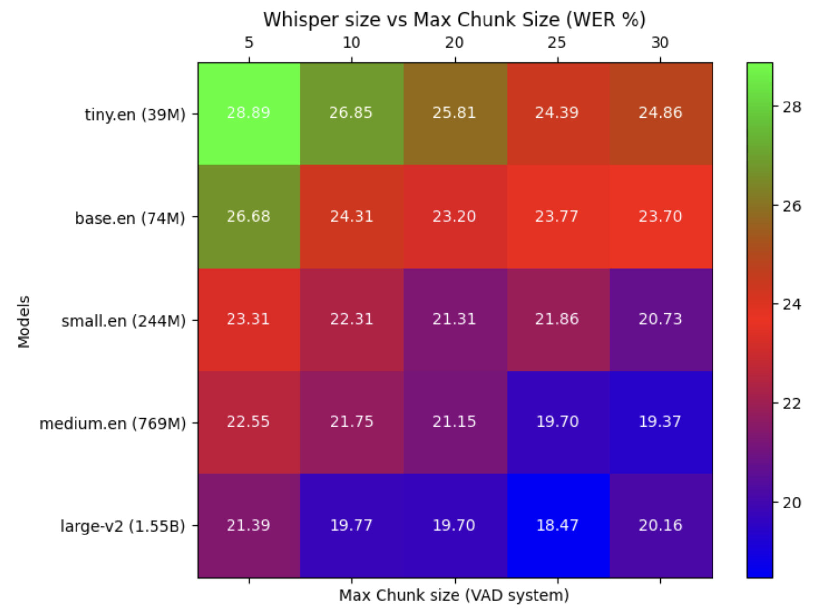
Figure 5: WERs on the test set with different Whisper model configurations and chunk sizes of the VAD model.

D.3 Filtering Stage

We perform an exhaustive filtering stage to remove potential low-quality data. This step further reduces the dataset to 510 hours, i.e., a 30% relative reduction. We use similar heuristics as in §3.1 to reduce the hallucinated hypotheses.

D.4 Additional supervised data

We use GigaSpeech Chen et al. (2021) (GS) L subset (2.5k hours), full LibriSpeech Panayotov et al. (2015) (LS) train set and CommonVoice English Ardila et al. (2020) (CV) train subset (1.5k hours) as extra datasets during training. This aims to regularize the training phase. In total, we use 5k hours of speech as extra datasets, while 510 hours are set as the target domain set.

D.5 Pseudo-labeled data filtering

As we aim to develop an ASR system as fast as possible, we developed a process to select a subset of the PL database smartly. We extract acoustic and text-based metadata from each $\{X,Y^{*}\}$ pair. The acoustic metrics (1) STOI, PESQ and SI-SDR are computed with TorchAaudio-SQUIM Kumar et al. (2023); (2) perplexity is computed with GPT2 Radford et al. (2019) using HuggingFace Wolf et al. (2020); Lhoest et al. (2021) and (3) a pseudo-edit-distance metric computed by comparing different Whisper model outputs, i.e., WER metric: whisper-tiny:hypothesis & whisper-large-v2:reference.

D.6 Experiments

We perform two experiments for the call center use case. First, in the baseline scenario, we filter out (or select) a subset from the original PL dataset by using one or multiple metrics, e.g., perplexity and SI-SDR threshold. We use the remaining dataset for ASR training. Second, we are presented with a fixed computational budget that limits the final dataset size for model training. This leads us to select a smaller portion of the PL dataset based on i) random selection or ii) sorting the PL dataset by one metric (e.g., SI-DR) and then selecting the top samples that meet the allowed computational budget.

Appendix E Data Selection Based on Metrics

This is the baseline scenario, where we filter the PL dataset by one or multiple metrics, and then we use the remaining dataset for ASR training. The results of this approach are listed in Table 6. Experiment 0) shows the WERs when using all the PL dataset, which serves as the baseline. From Exp 1) to 5) we run several filtering strategies, with some proposed metrics. Furthermore, we note that Exp 3) shows the best WERs while using 25% less data than Exp 0). This translates to faster training and convergence of the Zipformer model. In conclusion, these early experiments indicate that better WERs can be attained with fewer data points when a smart policy is in place. For instance, 0.5% absolute WER reduction, i.e., 13.9% WER (Exp 0) $\rightarrow$ 13.4% WER (Exp 3) from Table 6.

Table 6: WERs for Zipformer models trained for 20 epochs with different data selection policies. Note that all experiments use the multi-dataset training recipe unless otherwise specified. ^†Metric computed from comparing hypothesis between Whisper tiny and large-v2.

Exp	Data selection policy					Dataset	WER
	PPL	STOI	SI-SDR	WER†	BLEU	Size
-)	ALL data (no additional data)					510	15.1
0)	ALL data (baseline model)					510	13.9
1)	$\leq$ 500	$\leq$ 0.7	$\geq$ 15	-	-	210	15.1
2)	$\leq$ 800	$\leq$ 0.3	$\geq$ 5	-	-	437	13.5
3)	-	-	-	$\leq$ 25%	-	387	13.4
4)	-	-	-	-	$\geq$ 50	428	13.9

Fixed Computational Budget

In this setting, we are presented with a fixed computational budget, i.e., limited by the dataset sized for model training. This leads to selecting a smaller portion of the PL dataset based on i) random selection or ii) sorting the PL dataset by one metric (e.g., SI-DR) and then selecting the top samples meeting the allowed budget. These results are listed in Table 7. We can see significant WERs improvements up to the 200h of training. After this point, bringing more PL data at training time does not improve significantly WERs. In addition, we can conclude that none of the proposed sorting metrics is significantly better than random selection for ASR training when a fixed computational budget is imposed. There are several hypotheses that can justify these results, as follows:

1. The amount of PL data brings more WERs reductions than the proposed sorting metrics;

2. pseudo-labels from Whisper large-v2 are of sufficiently good quality, close to gold annotation levels;

3. the filtering stage is already removing most of the noisy and/or hallucinated PLs, i.e., the remaining 510-hour subset is already of good quality overall;

4. the proposed sorting metrics are not sufficiently discriminative for selecting the data required for the downstream application, i.e., random selection leads to lower WERs in some cases;

5. using supervised data at training time brings important regularization, thus minimizing the issue of using noisy PLs.

Table 7: WERs for Zipformer models trained for 10 epochs with different computational budgets w.r.t amount of data. ^†delta of relative WER reduction 50h $\rightarrow$ 400h.

	Sorting	Dataset size					$\Delta^{\dagger}$
	Metric	50h	100h	200h	300h	400h
0)	ALL data (baseline)	[510h] 13.9% WER
1)	WER ($\downarrow$)	30.7	19.3	15.3	15.0	13.8	55%
2)	Perplexity ($\downarrow$)	31.3	21.3	17.2	14.6	14.0	55%
3)	STOI ($\uparrow$)	33.0	21.7	16.6	15.9	13.9	57%
4)	Random selection	30.0	19.7	14.9	14.2	13.9	53%

The filtering stage is key for model training.  We confirmed this hypothesis by training a Zipformer model with multi-dataset training on the unfiltered PL dataset, i.e., a 735-hour subset. To our surprise, the model performance, even though seeing more data than Exp 0 (Table 7 and Table 6), did not reach acceptable WERs, e.g., 30%+ WER. Further research down this line will shed light on what are the best practices for selecting representative data for training, including filtering of hallucinated PLs. Note that selecting or sorting PLs might be of less importance as the dataset size increases.

References

- Aho and Corasick (1975) Alfred V Aho and Margaret J Corasick. 1975. Efficient string matching: an aid to bibliographic search. Communications of the ACM, 18(6):333–340.
- Aleksic et al. (2015) Petar Aleksic, Mohammadreza Ghodsi, et al. 2015. Bringing contextual information to google speech recognition. In Interspeech, pages 468–472.
- Ardila et al. (2020) Rosana Ardila, Megan Branson, Kelly Davis, Michael Kohler, Josh Meyer, Michael Henretty, Reuben Morais, Lindsay Saunders, Francis Tyers, and Gregor Weber. 2020. Common voice: A massively-multilingual speech corpus. In Proceedings of the Twelfth Language Resources and Evaluation Conference, pages 4218–4222.
- Armengol-Estapé et al. (2021) Jordi Armengol-Estapé, Casimiro Pio Carrino, Carlos Rodriguez-Penagos, Ona de Gibert Bonet, Carme Armentano-Oller, Aitor Gonzalez-Agirre, Maite Melero, and Marta Villegas. 2021. Are multilingual models the best choice for moderately under-resourced languages? A comprehensive assessment for Catalan. In Findings of the Association for Computational Linguistics: ACL-IJCNLP 2021, pages 4933–4946, Online. Association for Computational Linguistics.
- Baevski et al. (2020) Alexei Baevski, Yuhao Zhou, Abdelrahman Mohamed, and Michael Auli. 2020. wav2vec 2.0: A framework for self-supervised learning of speech representations. Advances in neural information processing systems, 33:12449–12460.
- Bain et al. (2023) Max Bain, Jaesung Huh, Tengda Han, and Andrew Zisserman. 2023. WhisperX: Time-Accurate Speech Transcription of Long-Form Audio. In Proc. INTERSPEECH 2023, pages 4489–4493.
- Barrault et al. (2023) Loïc Barrault, Yu-An Chung, Mariano Cora Meglioli, David Dale, Ning Dong, Paul-Ambroise Duquenne, Hady Elsahar, Hongyu Gong, Kevin Heffernan, John Hoffman, et al. 2023. Seamlessm4t-massively multilingual & multimodal machine translation. arXiv preprint arXiv:2308.11596.
- Bartelds et al. (2023) Martijn Bartelds, Nay San, Bradley McDonnell, Dan Jurafsky, and Martijn Wieling. 2023. Making more of little data: Improving low-resource automatic speech recognition using data augmentation. In Proceedings of the 61st Annual Meeting of the Association for Computational Linguistics (Volume 1: Long Papers), pages 715–729, Toronto, Canada. Association for Computational Linguistics.
- Battenberg et al. (2017) Eric Battenberg, Jitong Chen, Rewon Child, Adam Coates, Yashesh Gaur Yi Li, Hairong Liu, Sanjeev Satheesh, Anuroop Sriram, and Zhenyao Zhu. 2017. Exploring neural transducers for end-to-end speech recognition. In 2017 IEEE automatic speech recognition and understanding workshop (ASRU), pages 206–213. IEEE.
- Berrebbi et al. (2022) Dan Berrebbi, Ronan Collobert, Samy Bengio, Navdeep Jaitly, and Tatiana Likhomanenko. 2022. Continuous pseudo-labeling from the start. In The Eleventh International Conference on Learning Representations.
- Chebotar and Waters (2016) Yevgen Chebotar and Austin Waters. 2016. Distilling Knowledge from Ensembles of Neural Networks for Speech Recognition. In Proc. Interspeech 2016, pages 3439–3443.
- Chen et al. (2021) Guoguo Chen, Shuzhou Chai, Guan-Bo Wang, Jiayu Du, Wei-Qiang Zhang, Chao Weng, Dan Su, Daniel Povey, Jan Trmal, Junbo Zhang, Mingjie Jin, Sanjeev Khudanpur, Shinji Watanabe, Shuaijiang Zhao, Wei Zou, Xiangang Li, Xuchen Yao, Yongqing Wang, Zhao You, and Zhiyong Yan. 2021. GigaSpeech: An Evolving, Multi-Domain ASR Corpus with 10,000 Hours of Transcribed Audio. In Proc. Interspeech 2021, pages 3670–3674.
- Chen et al. (2019) Zhehuai Chen, Mahaveer Jain, Yongqiang Wang, Michael L Seltzer, and Christian Fuegen. 2019. End-to-end contextual speech recognition using class language models and a token passing decoder. In Proc. of IEEE International Conference on Acoustics, Speech and Signal Processing (ICASSP), pages 6186–6190. IEEE.
- Chiu et al. (2022) Chung-Cheng Chiu, James Qin, Yu Zhang, Jiahui Yu, and Yonghui Wu. 2022. Self-supervised learning with random-projection quantizer for speech recognition. In International Conference on Machine Learning, pages 3915–3924. PMLR.
- Conneau et al. (2020) Alexis Conneau, Alexei Baevski, Ronan Collobert, Abdelrahman Mohamed, and Michael Auli. 2020. Unsupervised cross-lingual representation learning for speech recognition. arXiv preprint arXiv:2006.13979.
- Ferraz et al. (2024) Thomas Palmeira Ferraz, Marcely Zanon Boito, Caroline Brun, and Vassilina Nikoulina. 2024. Multilingual distilwhisper: Efficient distillation of multi-task speech models via language-specific experts. In ICASSP 2024-2024 IEEE International Conference on Acoustics, Speech and Signal Processing (ICASSP).
- Gandhi et al. (2023) Sanchit Gandhi, Patrick von Platen, and Alexander M Rush. 2023. Distil-whisper: Robust knowledge distillation via large-scale pseudo labelling. arXiv preprint arXiv:2311.00430.
- Gao et al. (2023) Dongji Gao, Matthew Wiesner, Hainan Xu, Leibny Paola Garcia, Daniel Povey, and Sanjeev Khudanpur. 2023. Bypass temporal classification: Weakly supervised automatic speech recognition with imperfect transcripts. arXiv preprint arXiv:2306.01031.
- Ghodsi et al. (2020) Mohammadreza Ghodsi, Xiaofeng Liu, James Apfel, Rodrigo Cabrera, and Eugene Weinstein. 2020. Rnn-transducer with stateless prediction network. In ICASSP, pages 7049–7053. IEEE.
- Graves (2012) Alex Graves. 2012. Sequence transduction with recurrent neural networks. arXiv preprint arXiv:1211.3711.
- Graves et al. (2006) Alex Graves, Santiago Fernández, Faustino J. Gomez, and Jürgen Schmidhuber. 2006. Connectionist temporal classification: labelling unsegmented sequence data with recurrent neural networks. In Machine Learning, Proceedings of the Twenty-Third International Conference (ICML 2006), Pittsburgh, Pennsylvania, USA, June 25-29, 2006, volume 148 of ACM International Conference Proceeding Series, pages 369–376. ACM.
- Guo et al. (2023) Yachao Guo, Zhibin Qiu, Hao Huang, and Chng Eng Siong. 2023. Improved keyword recognition based on aho-corasick automaton. In 2023 International Joint Conference on Neural Networks (IJCNN), pages 1–7. IEEE.
- Higuchi et al. (2021) Yosuke Higuchi, Niko Moritz, Jonathan Le Roux, and Takaaki Hori. 2021. Momentum Pseudo-Labeling for Semi-Supervised Speech Recognition. In Proc. Interspeech 2021, pages 726–730.
- Hinton et al. (2015) Geoffrey Hinton, Oriol Vinyals, and Jeff Dean. 2015. Distilling the knowledge in a neural network. arXiv preprint arXiv:1503.02531.
- Hsu et al. (2021) Wei-Ning Hsu, Yao-Hung Hubert Tsai, Benjamin Bolte, Ruslan Salakhutdinov, and Abdelrahman Mohamed. 2021. Hubert: How much can a bad teacher benefit asr pre-training? In ICASSP 2021-2021 IEEE International Conference on Acoustics, Speech and Signal Processing (ICASSP), pages 6533–6537. IEEE.
- Jung et al. (2022) Namkyu Jung, Geonmin Kim, and Joon Son Chung. 2022. Spell my name: keyword boosted speech recognition. In ICASSP, pages 6642–6646. IEEE.
- Kannan et al. (2018) Anjuli Kannan, Yonghui Wu, Patrick Nguyen, Tara N Sainath, Zhijeng Chen, and Rohit Prabhavalkar. 2018. An analysis of incorporating an external language model into a sequence-to-sequence model. In ICASSP, pages 1–5828. IEEE.
- Kingma and Ba (2014) Diederik P Kingma and Jimmy Ba. 2014. Adam: A method for stochastic optimization. arXiv preprint arXiv:1412.6980.
- Kuang et al. (2022) Fangjun Kuang, Liyong Guo, Wei Kang, Long Lin, Mingshuang Luo, Zengwei Yao, and Daniel Povey. 2022. Pruned rnn-t for fast, memory-efficient asr training. arXiv preprint arXiv:2206.13236.
- Kumar et al. (2023) Anurag Kumar, Ke Tan, Zhaoheng Ni, Pranay Manocha, Xiaohui Zhang, Ethan Henderson, and Buye Xu. 2023. Torchaudio-squim: Reference-less speech quality and intelligibility measures in torchaudio. In ICASSP 2023-2023 IEEE International Conference on Acoustics, Speech and Signal Processing (ICASSP), pages 1–5. IEEE.
- Kumar et al. (2024) Shashi Kumar, Srikanth Madikeri, Juan Zuluaga-Gomez, Easu Villatoro-Tello, , Iuliia Nigmatulina, Petr Motlicek, K E Manjunath, and Aravind Ganapathiraju. 2024. XLSR-Transducer: Streaming ASR for Self-Supervised Pretrained Models. In Submitted to INTERSPEECH 2024.
- Kurata and Saon (2020) Gakuto Kurata and George Saon. 2020. Knowledge distillation from offline to streaming rnn transducer for end-to-end speech recognition. In Interspeech, pages 2117–2121.
- Lhoest et al. (2021) Quentin Lhoest, Albert Villanova del Moral, Yacine Jernite, Abhishek Thakur, Patrick von Platen, Suraj Patil, Julien Chaumond, Mariama Drame, Julien Plu, Lewis Tunstall, et al. 2021. Datasets: A community library for natural language processing. arXiv preprint arXiv:2109.02846.
- Li et al. (2020) Bo Li, Shuo-yiin Chang, Tara N Sainath, Ruoming Pang, Yanzhang He, Trevor Strohman, and Yonghui Wu. 2020. Towards fast and accurate streaming end-to-end asr. In ICASSP, pages 6069–6073. IEEE.
- Li et al. (2021) Bo Li, Anmol Gulati, Jiahui Yu, Tara N Sainath, Chung-Cheng Chiu, Arun Narayanan, Shuo-Yiin Chang, Ruoming Pang, Yanzhang He, James Qin, et al. 2021. A better and faster end-to-end model for streaming asr. In ICASSP, pages 5634–5638. IEEE.
- Likhomanenko et al. (2022) Tatiana Likhomanenko, Ronan Collobert, Navdeep Jaitly, and Samy Bengio. 2022. Continuous soft pseudo-labeling in asr. In I Can’t Believe It’s Not Better Workshop: Understanding Deep Learning Through Empirical Falsification.
- Lugosch et al. (2022) Loren Lugosch, Tatiana Likhomanenko, Gabriel Synnaeve, and Ronan Collobert. 2022. Pseudo-labeling for massively multilingual speech recognition. In ICASSP 2022-2022 IEEE International Conference on Acoustics, Speech and Signal Processing (ICASSP), pages 7687–7691. IEEE.
- Noroozi et al. (2023) Vahid Noroozi, Somshubra Majumdar, Ankur Kumar, Jagadeesh Balam, and Boris Ginsburg. 2023. Stateful fastconformer with cache-based inference for streaming automatic speech recognition. arXiv preprint arXiv:2312.17279.
- Panayotov et al. (2015) Vassil Panayotov, Guoguo Chen, Daniel Povey, and Sanjeev Khudanpur. 2015. Librispeech: an ASR corpus based on public domain audio books. In International Conference on Acoustics, Speech and Signal Processing (ICASSP), pages 5206–5210. IEEE.
- Panchapagesan et al. (2021) Sankaran Panchapagesan, Daniel S Park, Chung-Cheng Chiu, Yuan Shangguan, Qiao Liang, and Alexander Gruenstein. 2021. Efficient knowledge distillation for rnn-transducer models. In ICASSP 2021-2021 IEEE International Conference on Acoustics, Speech and Signal Processing (ICASSP), pages 5639–5643. IEEE.
- Park et al. (2019) Daniel S. Park, William Chan, Yu Zhang, Chung-Cheng Chiu, Barret Zoph, Ekin D. Cubuk, and Quoc V. Le. 2019. SpecAugment: A Simple Data Augmentation Method for Automatic Speech Recognition. In Proc. Interspeech 2019, pages 2613–2617.
- Prabhavalkar et al. (2023) Rohit Prabhavalkar, Takaaki Hori, Tara N Sainath, Ralf Schlüter, and Shinji Watanabe. 2023. End-to-end speech recognition: A survey. IEEE/ACM Transactions on Audio, Speech, and Language Processing.
- Pratap et al. (2023) Vineel Pratap, Andros Tjandra, Bowen Shi, Paden Tomasello, Arun Babu, Sayani Kundu, Ali Elkahky, Zhaoheng Ni, Apoorv Vyas, Maryam Fazel-Zarandi, et al. 2023. Scaling speech technology to 1,000+ languages. arXiv preprint arXiv:2305.13516.
- Radford et al. (2022) Alec Radford, Jong Wook Kim, Tao Xu, Greg Brockman, Christine McLeavey, and Ilya Sutskever. 2022. Robust speech recognition via large-scale weak supervision. ArXiv preprint, abs/2212.04356.
- Radford et al. (2019) Alec Radford, Jeffrey Wu, Rewon Child, David Luan, Dario Amodei, Ilya Sutskever, et al. 2019. Language models are unsupervised multitask learners. OpenAI blog, 1(8):9.
- Rekesh et al. (2023) Dima Rekesh, Nithin Rao Koluguri, Samuel Kriman, Somshubra Majumdar, Vahid Noroozi, He Huang, Oleksii Hrinchuk, Krishna Puvvada, Ankur Kumar, Jagadeesh Balam, et al. 2023. Fast conformer with linearly scalable attention for efficient speech recognition. In 2023 IEEE Automatic Speech Recognition and Understanding Workshop (ASRU), pages 1–8. IEEE.
- Sainath et al. (2020) Tara N Sainath, Yanzhang He, Bo Li, Arun Narayanan, Ruoming Pang, Antoine Bruguier, Shuo-yiin Chang, Wei Li, Raziel Alvarez, Zhifeng Chen, et al. 2020. A streaming on-device end-to-end model surpassing server-side conventional model quality and latency. In ICASSP 2020-2020 IEEE International Conference on Acoustics, Speech and Signal Processing (ICASSP), pages 6059–6063. IEEE.
- Stolcke (2002) Andreas Stolcke. 2002. Srilm-an extensible language modeling toolkit. In Seventh international conference on spoken language processing.
- Swietojanski et al. (2023) Pawel Swietojanski, Stefan Braun, et al. 2023. Variable attention masking for configurable transformer transducer speech recognition. In ICASSP, pages 1–5. IEEE.
- Takashima et al. (2018) Ryoichi Takashima, Sheng Li, and Hisashi Kawai. 2018. An investigation of a knowledge distillation method for ctc acoustic models. In 2018 IEEE International Conference on Acoustics, Speech and Signal Processing (ICASSP), pages 5809–5813. IEEE.
- Tedeschi et al. (2021) Simone Tedeschi, Valentino Maiorca, Niccolò Campolungo, Francesco Cecconi, and Roberto Navigli. 2021. WikiNEuRal: Combined neural and knowledge-based silver data creation for multilingual NER. In Findings of the Association for Computational Linguistics: EMNLP 2021, pages 2521–2533, Punta Cana, Dominican Republic. Association for Computational Linguistics.
- Vaswani et al. (2017) Ashish Vaswani, Noam Shazeer, Niki Parmar, Jakob Uszkoreit, Llion Jones, Aidan N Gomez, Łukasz Kaiser, and Illia Polosukhin. 2017. Attention is all you need. Advances in neural information processing systems, 30.
- Watanabe et al. (2017a) Shinji Watanabe, Takaaki Hori, Suyoun Kim, John R Hershey, and Tomoki Hayashi. 2017a. Hybrid ctc/attention architecture for end-to-end speech recognition. IEEE Journal of Selected Topics in Signal Processing, 11(8):1240–1253.
- Watanabe et al. (2017b) Shinji Watanabe, Takaaki Hori, Jonathan Le Roux, and John R Hershey. 2017b. Student-teacher network learning with enhanced features. In 2017 IEEE International Conference on Acoustics, Speech and Signal Processing (ICASSP), pages 5275–5279. IEEE.
- Wolf et al. (2020) Thomas Wolf, Lysandre Debut, Victor Sanh, Julien Chaumond, Clement Delangue, Anthony Moi, Pierric Cistac, Tim Rault, Rémi Louf, Morgan Funtowicz, et al. 2020. Transformers: State-of-the-art natural language processing. In Proceedings of the 2020 conference on empirical methods in natural language processing: system demonstrations, pages 38–45.
- Yang et al. (2022a) Haichuan Yang, Yuan Shangguan, Dilin Wang, Meng Li, Pierce Chuang, Xiaohui Zhang, Ganesh Venkatesh, Ozlem Kalinli, and Vikas Chandra. 2022a. Omni-sparsity dnn: Fast sparsity optimization for on-device streaming e2e asr via supernet. In ICASSP 2022-2022 IEEE International Conference on Acoustics, Speech and Signal Processing (ICASSP), pages 8197–8201. IEEE.
- Yang et al. (2022b) Xiaoyu Yang, Qiujia Li, and Philip C Woodland. 2022b. Knowledge distillation for neural transducers from large self-supervised pre-trained models. In ICASSP 2022-2022 IEEE International Conference on Acoustics, Speech and Signal Processing (ICASSP), pages 8527–8531. IEEE.
- Yao et al. (2023) Zengwei Yao, Liyong Guo, Xiaoyu Yang, Wei Kang, Fangjun Kuang, Yifan Yang, Zengrui Jin, Long Lin, and Daniel Povey. 2023. Zipformer: A faster and better encoder for automatic speech recognition. arXiv preprint arXiv:2310.11230.
- Yeh et al. (2019) Ching-Feng Yeh, Jay Mahadeokar, Kaustubh Kalgaonkar, Yongqiang Wang, Duc Le, Mahaveer Jain, Kjell Schubert, Christian Fuegen, and Michael L Seltzer. 2019. Transformer-transducer: End-to-end speech recognition with self-attention. arXiv preprint arXiv:1910.12977.
- Zavaliagkos and Colthurst (1998) George Zavaliagkos and Thomas Colthurst. 1998. Utilizing untranscribed training data to improve perfomance. In LREC, pages 317–322. Citeseer.
- Żelasko et al. (2021) Piotr Żelasko, Daniel Povey, Jan Trmal, Sanjeev Khudanpur, et al. 2021. Lhotse: a speech data representation library for the modern deep learning ecosystem. arXiv preprint arXiv:2110.12561.
- Zhang et al. (2020) Qian Zhang, Han Lu, Hasim Sak, Anshuman Tripathi, Erik McDermott, Stephen Koo, and Shankar Kumar. 2020. Transformer transducer: A streamable speech recognition model with transformer encoders and rnn-t loss. In ICASSP, pages 7829–7833. IEEE.
- Zhao et al. (2019) Ding Zhao, Tara N Sainath, David Rybach, Pat Rondon, Deepti Bhatia, Bo Li, and Ruoming Pang. 2019. Shallow-fusion end-to-end contextual biasing. In Interspeech, pages 1418–1422.
- Zhu et al. (2023) Han Zhu, Dongji Gao, Gaofeng Cheng, Daniel Povey, Pengyuan Zhang, and Yonghong Yan. 2023. Alternative pseudo-labeling for semi-supervised automatic speech recognition. IEEE/ACM Transactions on Audio, Speech, and Language Processing.
- Zuluaga-Gomez et al. (2021) Juan Zuluaga-Gomez, Iuliia Nigmatulina, Amrutha Prasad, Petr Motlicek, Karel Veselý, Martin Kocour, and Igor Szöke. 2021. Contextual Semi-Supervised Learning: An Approach to Leverage Air-Surveillance and Untranscribed ATC Data in ASR Systems. In Proc. Interspeech, pages 3296–3300.
- Zuluaga-Gomez et al. (2023) Juan Zuluaga-Gomez, Amrutha Prasad, Iuliia Nigmatulina, Seyyed Saeed Sarfjoo, Petr Motlicek, Matthias Kleinert, Hartmut Helmke, Oliver Ohneiser, and Qingran Zhan. 2023. How does pre-trained wav2vec 2.0 perform on domain-shifted asr? an extensive benchmark on air traffic control communications. In 2022 IEEE Spoken Language Technology Workshop (SLT), pages 205–212. IEEE.