Abstract

This paper presents results of the first full simulation study addressing prospects for observation of long-lived particles (LLPs) with the International Large Detector (ILD). Neutral LLP production, resulting in a displaced vertex signature inside the ILD’s time projection chamber (TPC), is considered. We focus on scenarios interesting from the experimental perspective and perform a search based on displaced vertex finding inside the TPC volume. Two experimentally very challenging types of scenarios are explored: first, involving very soft final states due to a small mass splitting between heavy LLP and a dark matter particle to which the LLP decays, and the second one, with a light LLP production resulting in almost colinear vertex tracks because of a large boost of the LLP. The expected limits on the signal production cross section are presented for a wide range of the LLP proper lifetimes corresponding to $c\tau$ from 0.1 mm to 10 km.

1 Introduction

The Standard Model (SM) of particle physics [1, 2, 3, 4, 5, 6] provides a comprehensive framework for understanding the interactions among constituents of the Universe discovered so far. Despite its remarkable success [7, 8, 9, 10, 11, 12], there is a number of theoretical and experimental indications, prompting a search for new physics phenomena Beyond the SM (BSM), such as Dark Matter (DM) particles, additional sources of the CP violation, or an origin of neutrino masses. An interesting case explored in many recent studies involves a concept of new Long-Lived Particles (LLPs), i.e. BSM particles characterized by their macroscopic lifetimes (of the order of picoseconds or higher). One should realize that many such states occur within the SM already (neutrons, muons, kaons, pions, etc.) so there is no explicit reason to expect that all hypothetical BSM particles should decay promptly. States with macroscopic lifetimes naturally appear in many BSM models [13, 14, 15, 16, 17], and if existed, they could evade many of the standard new physics searches conducted e.g. at the Large Hadron Collider (LHC). A dedicated event reconstruction and selection approach is needed to search for LLP production, targeting unique signatures such as displaced vertices (with tracks or jets in the final state), disappearing or kinked tracks, strongly ionising charged particles, non-pointing photons, and more [18].

Although LLPs have already been considered in a variety of BSM searches at the LHC, no indication for LLP production has been observed so far. The ATLAS and CMS experiments have probed large parts of the parameter space, imposing strong constraints on very massive LLPs for a wide range of lifetimes. Searches for decays inside the muon systems allowed probing decay lengths above 500 m for LLP masses of 40 GeV [19, 20], while considering delayed decays constrains the proper decay lengths even at the order of $10^{12}$ m [21]. Huge masses of up to 2.5 TeV have also been probed in searches for displaced jets [22] and up to 1.8 TeV using a displaced vertex with missing momentum signature [23, 24]. Also, an opposite corner of kinematic parameter space with lighter LLPs started to gain more interest recently. Models with LLP masses as small as 400 MeV have been constrained at the LHC in Higgs boson decays [19, 25] and a recent search for displaced muon pairs probes heavy squark decays to long-lived neutralinos, where the mass splitting between those two is only 25 GeV [26]. However, in this regime experiments at the LHC suffer from a huge background, which can affect searches for both light and heavier states, in particular in the case of models with compressed spectra (small mass differences between particles in the decay chain). In order to gain sensitivity, light LLPs must originate from decays of much heavier particles, or the analysis must rely on some model-specific assumptions.

Small couplings and compressed spectra are exactly the features leading to predictions of the LLPs by theoretical models [27], so there is a strong motivation for testing this region beyond the current LHC reach. The recent growing interest in models with the so-called feebly interacting massive particles (FIMPs), which often exhibit macroscopic lifetimes or appear alongside the LLPs, also points in this direction [28]. This could be addressed by the future Higgs factories, where the LHC searches for LLPs could be complemented.

According to the last 2020 Update of the European Strategy for Particle Physics, an e⁺e^- Higgs factory is “the highest-priority next collider" [29]. Currently, there are several proposals for such a machine, and the most studied concepts are: The International Linear Collider (ILC) [30], The Compact Linear Collider (CLIC) [31], The Future Circular Collider (FCC-ee) [32], and The Circular Electron Positron Collider (CEPC) [33]. In this paper, we consider the ILC as a “reference collider", since it remains the most mature option, with the Technical Design Report published in 2013 [34]. The ILC baseline running scenario (H20) assumes staged operation at two center-of-mass energies (250 and 500 GeV), with the electron and positron beams polarized longitudinally and luminosity sharing between the four beam helicity configurations. A total of 2 ab^-1 and 4 ab^-1 integrated luminosity is planned to be collected at the 250 and 500 GeV stages, respectively. The ILC operation at the Z-pole (ILC-GigaZ) and an upgrade to $\sqrt{s}=1$ TeV are also possible [30].

Although their primary goals are precision measurements of the Higgs boson, top quark, and the electroweak sector, future e⁺e^- colliders, with a clean experimental environment and triggerless operation are also very well suited to look for uncommon signatures and exotic phenomena. Prospects for the LLP searches at future Higgs factories are one of the focus topics of the ongoing ECFA study [35]. Very promising in this context is the International Large Detector (ILD) concept [36], which was originally proposed as one of the experiments for the ILC, although studies are currently ongoing regarding its possible operation at a circular machine.

The ILD tracking system comprises of five subdetectors. The vertex detector (VTX), located closest to the beam pipe, consists of three double layers of silicon pixel sensors. In the central region it is surrounded by two double layers of a silicon internal tracker (SIT), and in the forward region it is extended by seven discs (five of which are double discs) of the forward tracking detectors (FTD). The FTD acceptance starts already at an angle of 4.8 degrees. The main tracker of the ILD is a time projection chamber (TPC) allowing for almost continuous tracking, which can significantly enhance the reach in searches for displaced signatures [37]. In addition, the TPC is surrounded by one double layer of a strip silicon external tracker (SET). The ILD baseline design is optimized for event reconstruction with the particle-flow approach [38] based on highly granular calorimeters. For details about the ILD see Ref. [36] and references therein.

For these reasons, this paper focuses on scenarios including light particles and soft final states not (fully) tested at the LHC. Since most of LLP signatures involve uncommon track topologies (one or multiple tracks with high displacement or large impact parameter), we consider just two tracks originating from a displaced vertex as a generic case. An inclusive analysis is performed, with the selection not optimized for any particular BSM scenario or a specific signature. This is discussed in more detail in Section 2, together with the experiment-orientated approach taken in this study and the selected benchmark scenarios. Section 3 describes beam-induced backgrounds and measures proposed for their reduction, which are followed by a selection aimed to reduce backgrounds from other SM processes, introduced in Section 4. Section 5 presents the performance of a vertex finding procedure developed for this analysis, resulting in the limits on signal production cross section shown in Section 6. The study is summarized in Section 7.

2 Benchmark scenarios and analysis strategy

We study prospects for the LLP observation at future colliders from an experimental point of view. Discussed in this paper are two scenarios of LLP production – light LLP resulting in boosted, high-$p_{T}$ SM final state, and (relatively) heavy LLP, which decays to a heavy DM particle and to SM particles. The benchmark scenarios are not selected based on any particular theoretical model and existing experimental constraints in its parameter space, but rather as those providing signatures interesting from the experimental perspective – potentially challenging or not accessible at the LHC.

We identify three factors that can limit sensitivity to LLP production: soft (but very numerous) beam-induced background, hard SM background, and detector or reconstruction limitations. Soft signals can be mimicked by the first of these backgrounds and the boosted topologies by the second one, while both scenarios are challenging for detectors and reconstruction techniques. Therefore, with this choice of benchmarks, we test all three potential limitations.

Following model-independent approach, we do not assume anything about the final state except for the presence of at least one displaced vertex inside the TPC, as the most generic case. Only two-prong vertices were considered, as it can be assumed that such a topology will be the most experimentally challenging one. Although multi-prong topology may bring its own analysis challenges, we expect that finding a displaced vertex with multiple tracks in the final state should not be less efficient than in case of having just two tracks, and the background levels, those coming from random track intersections in particular, should be much smaller. The vertex-finding procedure is described later in this section, and the selection of vertex candidates in the Sections 3 and 4 of this paper. We use particular models to generate samples for the analysis; however, we do not make any model-specific assumptions in the analysis, in order to make the results relevant for any model providing the considered, or similar, signatures.

The first class of analyzed scenarios involves low-$p_{T}$, little boosted tracks in the final state, whose combined momentum do not extrapolate close to the interaction point (IP). The model used to generate events with this signature was the Inert Doublet Model (IDM) [39], which introduces four additional scalars: H^±, A, and H, which could be both lighter and heavier than the SM-like 125 GeV scalar h. The lighter neutral scalar H is stable and is a DM candidate. The neutral scalars can be pair-produced in e⁺e^- collisions, with a predominant further decay of A $\to$ Z^(∗)H; this process is shown in Figure 1 (left). If the mass splitting, $\Delta m_{AH}=m_{A}-m_{H}$, between A and H is small, the Z boson is highly virtual and A can be long-lived due to the small decay phase space available. Because H is invisible and escapes undetected, only the Z^(∗) decay products are expected to be measured inside the detector. The small mass splitting and the sizable mass $m_{A}$ of the A boson implies that the final-state tracks are soft and are not pointing to the IP. We consider four benchmark scenarios with fixed LLP mass $m_{A}=75$ GeV and decay length $c\tau=1$ m, and different $\Delta m_{AH}=1,2,3,5$ GeV.

The second type of scenario under consideration was a production of a very light LLP, decaying into strongly boosted and almost colinear tracks. It was modelled using the photon-associated axion-like particle (ALP) production process, as shown in Fig. 1 (right). In many scenarios, ALPs having macroscopic lifetimes for $\mathcal{O}$(GeV) mass scales could be copiously produced in e⁺e^- collisions [40]. For this signature, we select four benchmarks as well, with ALP masses $m_{a}=0.3,1,3,10$ GeV and decay lengths $c\tau=10\cdot m_{a}$ mm/GeV to maintain large number of decays inside the detector volume.

Figure 1: Leading Feynman diagrams corresponding to the processes used to simulate the considered benchmark scenarios. Left: IDM neutral scalar pair-production with A as the LLP; H is invisible and Z boson is virtual for small $\Delta m_{AH}$. Right: Associated production of an ALP, a, with a photon where ALP can be long-lived.

For each scenario samples of 10,000 events were generated with Whizard 3.0.1 and 3.1.2 [41], for IDM and ALPs respectively, at the $\sqrt{s}=250$ GeV ILC. Full simulation of the detector response was based on the ILD-L detector model [36] implemented in the DD4hep [42] framework and interfaced with Geant4 [43]. Event samples were processed on the grid with the ILCDirac interface [44].

Only decays of ALPs and Z^(∗) to muon pairs were generated. This allowed for faster detector response simulation, since muons do not produce showers inside calorimeters as opposed to electrons or pions. However, it should be noted that this choice does not make our search less general, as displaced multi-track final states are also included in the analysis, despite the fact that we do not test them explicitly as the signal scenarios. As a result, we find that they constitute a significant background contribution from the SM events (see Sections 3 and 4 for details), but it confirms that using only muons for signal samples does not produce any significant bias.

Reconstruction was performed using iLCSoft v02-02-03 [45] and based on the Marlin framework [46]. The standard ILD reconstruction chain [47] was used, however, selection cuts based on impact parameters $d_{0}$, $z_{0}$ (in the XY plane and Z coordinate, respectively [48]) of the reconstructed tracks have not been applied at the final step of track reconstruction, in the FullLDCTracking processor [49]. For this study, we designed a dedicated procedure for vertex finding inside the TPC volume. It is meant to be as simple and general as possible. If a track starts inside the TPC, its direction (and hence the charge) is ambiguous, i.e. can be reconstructed as an oppositely charged track traveling in the other way. For this reason, for each pair of tracks in an event, the algorithm considers four possible hypotheses of the track directions. The hypothesis chosen is the one for which the tracks have opposite charges and the distance between their first hits is the smallest. Then, the vertex is placed in between the points of the closest approach of track helices, requiring the distance between the helices to be less than 25 mm. Schematic view of a vertex placement can be seen in Figure 3 (Sec. 3), which illustrates variables used for the selection.

The analysis is performed in an approach similar to an anomaly search, where the signal can take any form of tracks forming displaced vertices and a discovery would be implied by an excess in the number of reconstructed vertices. As shown in more detail in the following sections of the paper, the backgrounds hardly exhibit any process-dependent behavior, except for a distinction between low- and high-momenta events, and between processes with different numbers of objects expected in the final state. The vast majority of background sources originate from random coincidences of tracks, single neutral, long-lived SM particles, and secondary interactions with the detector material. Therefore, any SM process with a high cross section and a large activity inside the detector is a potential background source.

3 Beam-induced backgrounds

At linear e⁺e^- colliders the beams need to be very strongly focused at the IP, to reach the required luminosity. Consequently, the charge density at the IP is very high. Therefore, besides quasi-real photons radiated by individual electrons (as described by Weizsäcker-Williams approximation), bunches are accompanied by synchrotron radiation caused by an interaction with the opposite beam, the so-called beamstrahlung. Both quasi-real and beamstrahlung photons emitted by one of the bunches can interact with those from the opposite bunch. Hence, each bunch crossing (BX) at a linear collider is a source of low-$p_{T}$ hadron photoproduction ($\gamma\gamma\to$ hadrons) and incoherent e⁺e^- pairs due to beam-induced photon interactions. In the ILD operating at the 250 GeV ILC, around 1.55 $\gamma\gamma\to$ hadrons events are expected on average per BX. In addition, $\mathcal{O}(10^{5})$ incoherent pairs are produced per BX. However, they are predominantly emitted in the forward direction and only a small fraction of them enters the detector and can be measured. Both of these processes occur in the detector simultaneously with physical hard events (and hence they are typically called overlay events). However, with an order of $10^{11}$ BXs expected at the ILC per year, these events are a potential source of a standalone background, in particular for the signal scenarios considered in this study involving soft final states. Figure 2 (left) presents a distribution of displaced vertices as a function of the distance $R$ from the beam axis. There is an overwhelming number of vertices found in the overlay samples, most of which are fake (e.g. originate from randomly intersecting tracks). Figure 2 (right) shows the distribution of the total transverse momentum, $p_{T}^{vtx}$, of tracks forming displaced vertex candidate, compared for the overlay events and two of the considered signal scenarios. It can be noted that vertices in the overlay sample occupy the same kinematic region. These distributions show that $\gamma\gamma\to$ hadrons and incoherent e⁺e^- pairs events cannot be neglected as a background source in this study, and will require a dedicated mitigation strategy.

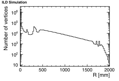
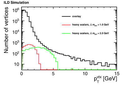
Figure 2: Left: Number of displaced vertices found in the overlay sample as a function of distance from the beam axis. Right: Total transverse momentum of tracks coming from a displaced vertex for the overlay (black) and scalar pair-production with $\Delta m_{AH}=1$ GeV (red) and $\Delta m_{AH}=2$ GeV (green). All histograms are normalized to the number of simulated events and correspond to no selection applied at all, just except for the required maximum distance between track helices.

Soft hadrons can be produced in photon-photon interactions both from beamstrahlung ($\gamma^{B}$) and from the Weizsäcker-Williams spectrum ($\gamma^{W}$), so four channels are possible. Number of events occurring per single BX for each of them is a random number from the Poisson distribution with a given mean, $\mu_{P}$, which is used in the standard ILD reconstruction chain when overlaying the background on signal events. Table 1 presents these expected values for the 250  GeV ILC, together with the number $N_{evt}$ of events used in this study for each channel. The incoherent e⁺e^- pairs are included in the analysis as well. To do so, 99,000 BXs were generated with GuineaPig [50]. For each of these BXs, only the incoherent pairs that would potentially hit any tracking detector were written out and were fully simulated. From this pool of BXs, one was picked at random for each physics event, and overlayed before reconstruction. This set of BXs was also used as a standalone background, similar to the hadron photoproduction.

Table 1: Average number, $\mu_{P}$, of overlay events expected per single BX for different channels and the number, $N_{evt}$, of corresponding events used in the analysis.

channel	$\mu_{P}$	$N_{evt}$
$\gamma^{B}\gamma^{B}$	0.8298	1,418,000
$\gamma^{B}\gamma^{W}$	0.2972	889,000
$\gamma^{W}\gamma^{B}$	0.2975	911,000
$\gamma^{W}\gamma^{W}$	0.1257	519,000
tot. $\gamma\gamma\to$ hadrons	1.55	3,837,000

3.1 Preliminary cuts

We apply three sets of preliminary cuts to reduce the number of fake vertices of different categories. The first set of cuts is based on variables describing track pair geometry and is aimed at reduction of nonphysical vertices coming from reconstruction inaccuracies or random coincidences.

• Sometimes a charged particle will scatter at unusually large angle at one point in the detector, and the standard track-reconstruction will split the track in two. Track splitting might also occur during reconstruction, when merging of a curling track segments fails. In this analysis, this would be interpreted as a displaced vertex at the point where the track was split. However, the two track segments will be close to colinear at the split-point, and the curvature of the segments will be close to identical. Therefore, we restrict the track pair opening angle $\alpha$ to $\cos{\alpha}>-0.6$ and the ratio of the curvature of the tracks to $\left|\Omega_{1}\right|/\left|\Omega_{2}\right|<0.94$, assuming $\left|\Omega_{1}\right|<\left|\Omega_{2}\right|$ (following definitions of helix parametrization in Ref. [48]).

• In some cases, reconstruction of one of the segments of a curling track fails completely, which can lead to formation of poor, short tracks, often with unexpectedly large $p_{T}$. Such tracks are more likely to pick up a second track in the event to form a vertex. To reject such vertices, it was required that both tracks should have the number of degrees of freedom in the track-fit exceeding 40, a number increased to 70 for the highest $p_{T}$ track of the vertex, if the $p_{T}$ was above 1.5 GeV.

• To further suppress vertices coming from accidental intersections of uncorrelated tracks, the vertex should be close to or before the first point measured on the track. To account for tracks with high $p_{T}$, almost perpendicular to the beam axis, as well as low-$p_{T}$ tracks curling many times along the Z axis, we use two complementary sets of cuts, depending on the distance $z_{12}=|z_{\mathrm{first}}-z_{\mathrm{last}}|$ between the first and the last track hit in the Z coordinate. For the tracks with $z_{12}\leq 100$ mm, the ratio of azimuthal angular distance $\phi_{1}$ from the vertex to the first hit, relative to the total angle $\phi_{arc}$ from the first to last hit of the track, $\phi_{1}/\phi_{arc}$, should not exceed 0.05 (see Figure 3). For the track with $z_{12}>100$ mm, the requirement is used for a difference $z_{1}=z_{\mathrm{first}}-z_{\mathrm{vtx}}$ in Z coordinate between the first hit and the vertex, relative to the $z_{12}$. Value of $\mathrm{sgn}(p_{z})\cdot z_{1}/z_{12}$ must be higher than $-0.01$, where $p_{z}$ is the Z component of the track momentum. Note that $z_{1}$ can be both positive and negative depending on the track direction, so with a perfect reconstruction of the vertex position, this expression should always be positive.

An important source of the background are interactions of both charged and neutral particles with the detector material producing (one or more) secondary, displaced tracks emerging from the displaced vertex. As we consider two hypotheses of direction for each track, a charged particle producing a single secondary track can look like a vertex as well, with one of the tracks going back into the IP. It is worth noting that it is a potential charged LLP signature explored in many searches that our vertex-finding procedure is also sensitive to. However, we focus on the neutral LLPs here and regard these vertices only as a part of the background. To remove such events a second set of requirements is imposed.

• The search region is restricted to the vertex radii in the 0.4-1.5 m range, since secondary interactions occur mainly (but not only) with the inner and outer walls of the TPC.

• Vertices resulting from the charged particles interaction with the detector material are first rejected by requiring no additional tracks that end within 30 mm of the vertex and no tracks with $d_{0}<10$ mm that pass 30 mm from the vertex.

• If at least one of the tracks at a vertex has $d_{0}<50$ mm we require that its first hit (the one closer to the reconstructed displaced vertex) has a smaller radius $R_{f}$ than its last hit $R_{l}$. This cut is targeting "kink" signatures: the vertex and secondary track reconstructed as an effect of scattering of charged particles.

The neutral particles producing two or more secondary tracks are considered as mostly irreducible background, partly mitigated by the first cut. That is due to the model-independent approach, in which we do not want to exclude scenarios with LLP decays to more than two charged particles, displaced jet signatures in particular, even though they are not analyzed as such.

Finally, with a third set of preselection cuts, we remove vertices corresponding to decays of V⁰ particles.

• Matching of vertex candidates with the output of a dedicated ILD processor for V⁰ identification is performed. The LLP vertex candidate is rejected if there is a vertex reconstructed by the processor closer than 30 mm.

• We exclude vertices with an invariant mass $M_{inv}^{\pi\pi}$ (assuming the tracks are pions) in a window of $\pm 50$ MeV around K⁰ mass and $M_{inv}^{\pi p/p\pi}$ (assuming one track is a pion and the other is a proton and vice versa) around $\Lambda^{0}$ mass.

• For the assumption that both tracks are electrons, we reject vertices with a mass $M_{inv}^{ee}$ less than 150 MeV. A wide window aims to account for poorly reconstructed and almost colinear tracks from highly displaced photon conversions.

Cuts on the invariant mass of a pair of tracks for different track mass hypotheses are required for more efficient background suppression as the processor for V⁰ identification has finite efficiency and prioritizes purity. With the overwhelming number of overlay events, the remaining V⁰ particles not identified by the algorithm still constitute a substantial background for rare processes.

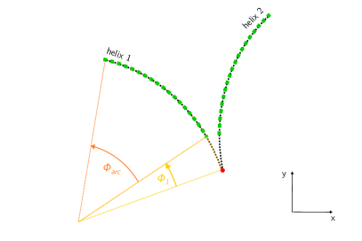
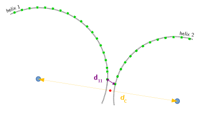
Figure 3: Schematic illustration of variables used for the overlay selection. Helix curves are represented by black dotted lines and detector hits by small green rectangles. Left: Projection of helices into XY plane and the angular variables $\phi_{1}$ and $\phi_{arc}$ used in the preselection. Right: Variables $d_{C}$ and $d_{11}$ that combined are used in the final selection. Small blue circles represent centers of projections of helices into XY plane. Note that $d_{11}$ is a three-dimensional distance. Red dot corresponds to a vertex candidate.

3.2 Final selection

The preliminary cuts described above allow for background reduction by a factor of around 500, down to the level of 0.21%. However, due to the huge expected number of BXs in a collider such as the ILC, a suppression factor at the level of at least 10^-9 or higher is needed to achieve good sensitivity to rare BSM signals. Since it is not possible to generate an event sample of a size corresponding to the expected number of BXs in the experiment, a direct determination of the reduction factor is not possible, and it can only be estimated assuming factorization, as a product of the subsequent selection cut efficiencies. However, this will only provide a reliable result if the variables used in the selection are statistically independent. Therefore, we select uncorrelated variables for the final selection cuts so that the total reduction factor can be obtained by multiplying all cut efficiencies.

We use two variables. The first is just the total transverse momentum $p_{T}^{vtx}$ of a pair of tracks, as the background is expected to occupy the region of very low $p_{T}$, as shown in the right plot of Figure 2. Tracks in the LLP signals should also come out of a single point, so distance $d_{11}$ (in three dimensions) between their first hits in the TPC should be small. On the other hand, helix-circles (projections of track helices onto the XY plane) of these tracks should not overlap, so the distance $d_{C}$ between their centers should be large. Schematic visualization of $d_{11}$ and $d_{C}$ is shown in Figure 3 (right). To reduce the number of selection criteria and avoid correlation between these two variables, we define a new variable $d_{h}\equiv 2.2d_{11}-d_{C}$, the distribution of which is shown in Figure 4 for the signal (left) and background (right) as a function of $p_{T}^{vtx}$, after the preliminary selection. The factor 2.2 is chosen as the best for most optimal signal-background separation. As visible in the distribution on the left, for true vertices the $d_{h}$ and $p_{T}^{vtx}$ variables are strongly correlated. However, only little to no correlation should be observed for any fake vertices from random coincidences remaining in the overlay sample, as can be seen in the right plot. We choose $d_{h}<-2000$ mm and $p_{T}^{vtx}>1.9$ GeV as the optimal cuts. To mitigate the effect of limited statistics, we estimate the reduction factor for each of those variables from distributions fitted to the respective histograms of $p_{T}^{vtx}$ and $d_{h}$. The functions used were, respectively, log-normal distribution for the $p_{T}$ and a sum of Crystal Ball functions, $c_{1}(x)+c_{2}(-x)$, for the $d_{h}$. This is performed for all overlay events that survive the preliminary selection, weighted by the corresponding expected values $\mu_{P}$ shown in Table 1. Cuts on the $p_{T}^{vtx}$ and $d_{h}$ result in selection efficiencies of $1.73\cdot 10^{-3}$ and $3.48\cdot 10^{-5}$, respectively. As each of those factors is determined on the sample of events after the preliminary cuts, this can be combined with the preliminary selection efficiency, which gives the total reduction factor of $1.26\cdot 10^{-10}$.

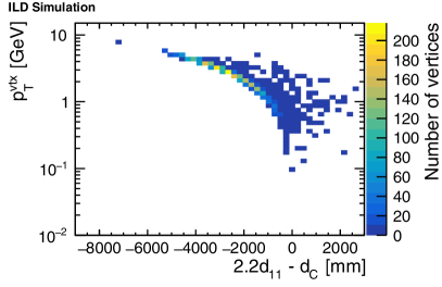
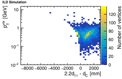
Figure 4: Distribution of $p_{T}^{vtx}$ as a function of $d_{h}$ variable for $\Delta m_{AH}=2$ GeV signal scenario (left) and all unweighted overlay events that survive the preliminary cuts (right). For the signal these variables show strong correlation, but for the background only very small correlations are visible for a few events at the lowest values of $d_{h}$. Both variables are used for the final selection aimed to suppress the background from overlay events; see text for details.

4 Backgrounds from physical events

The SM processes from hard e⁺e^- scattering (listed in Table 2 together with their cross sections at 250 GeV ILC) are also taken into account. Preliminary tests have shown that the main sources of displaced vertices in this case are, similar to overlay events, the interactions with the detector material and decays of long-lived hadrons, which happen predominantly inside the jets. Therefore, one could expect that the vertex finding rate for background, defined as a fraction of events with at least one identified vertex to all events, does not depend on a physical process itself and neither on the beam polarization, but rather on a number of jets produced. Because rerunning track reconstruction for all SM samples is very time and resource consuming, we obtain the selection efficiencies directly for the most significant processes (those with the highest cross sections), two-fermion (e⁺e^- $\to$ q$\bar{\mathrm{q}}$) and four-fermion (e⁺e^- $\to\mathrm{q\bar{q}q\bar{q}}$) hadronic channels. Then, to estimate the level of background for a complete set of SM processes, we use the q$\bar{\mathrm{q}}$ vertex finding rate for other e⁺e^- channels, as they also involve two jets in the final state. However, we also take into account the hard scattering of $\gamma^{B/W}\gamma^{B/W}$, which we simulate as well, since this background might in principle contain different sources of (fake) displaced vertices. Six-fermion production and e${}^{\pm}\gamma$ interactions were neglected because of much smaller cross sections.

Table 2: Cross sections for the SM processes at $\sqrt{s}=250$ GeV considered in this study, for different setups of the beam polarization, assuming $\pm 100\%$ polarization, and different photon sources for $\gamma\gamma$ processes.

sgn(P(e-), P(e+))	($-,+$)	($+,-$)	($-,-$)	($+,+$)
channel	$\sigma$ [fb]
qq	127,966	70,417	0	0
qqqq	28,660	970	0	0
qq$\ell\nu$	29,043	261	191	191
qq$\ell\ell$, qq$\nu\nu$	2715	1817	1,156	1,157
process	BB	BW	WB	WW
$\gamma^{B/W}\gamma^{B/W}$	42,150	90,338	90,120	71,506

First, q$\bar{\mathrm{q}}$ is considered as the dominant background, and the selection established for the reduction of overlay events is applied. To further reduce background from coincidences of random tracks within high $p_{T}$ hadronic jets, a separate cut on $d_{11}<50$ mm is applied. We will refer to this whole set of cuts as the standard selection. It yields the vertex finding rate of $(7.99\pm 0.68)\cdot 10^{-4}$ for the q$\bar{\mathrm{q}}$ sample. The rate obtained for the qqqq sample was found to be $(1.486\pm 0.094)\cdot 10^{-3}$, which is a factor of 1.86 greater, so it seems to confirm the assumption of rate dependence on the number of jets. For hard $\gamma^{B/W}\gamma^{B/W}$ scattering, the rate of $(2.13\pm 0.28)\cdot 10^{-5}$ was obtained. All uncertainties are statistical, calculated as $\sigma_{i}=\sqrt{\epsilon_{i}(1-\epsilon_{i})/N_{i}}$, where $\epsilon_{i}$ is the respective vertex finding rate, and $N_{i}$ is the total number of events in a sample.

Fully hadronic or leptonic decays of V⁰ particles are efficiently identified and rejected by the cuts described so far. However, this is not the case for semileptonic K${}^{0}_{\mathrm{L}}$ decays, since they involve neutrinos in the final state, resulting in smeared and shifted mass distribution. A similar effect can be due to large reconstruction uncertainties, for short or colimated tracks in particular. This is visible on distributions presented in Figure 5 for hypotheses that the tracks are electrons (left) and pions (right) after the standard selection. To further improve background rejection and final sensitivity to LLPs, we also define a tight selection with additional cuts. In this case, cuts in the electron- and pion-track mass hypotheses are extended to exclude all candidates with $M_{inv}^{ee},M_{inv}^{\pi\pi}<700$ MeV. The window in the cut on $\Lambda^{0}$ mass is reduced from $\pm 50$ MeV to $\pm 20$ MeV, since now it can significantly improve the signal selection efficiency without much increase in the background. In the tight selection, we also use the fact that final state tracks in the signal processes should be quite isolated from other activity in the event, while for the background, displaced vertices are mostly reconstructed inside the jets. The isolation measure is chosen as a scalar sum $p_{cone}=\Sigma_{i}|\vec{p}_{i}|$ of the track momenta in a cone spanned by an opening angle $\beta$ of $\cos{\beta}>0.98$, around the combined momentum $p_{vtx}$ of the track pair at the vertex. Tracks whose first or last hit is 30 mm within the vertex candidate are not included in the sum not to exclude vertices with more than two tracks in the final state. The distribution of $p_{cone}$ as a function of $p_{vtx}$ is presented in Figure 6 (left) for the q$\bar{\mathrm{q}}$ background and $\Delta m_{AH}=2,3$ GeV signal scenarios after the standard selection. To suppress background from displaced vertices reconstructed inside hadronic jets we require that $p_{cone}<1$ GeV. Because of this isolation criterion, the tight selection might be seen as partly model-dependent (some models could predict an LLP production within or close to hardonic jets). For this reason it is considered separately from the standard set of cuts. However, it is important to note that the vast majority of models currently considered do not predict an LLP production in association with close-by high-momentum tracks. Tight cuts on the $M_{inv}^{ee},M_{inv}^{\pi\pi}$, and on the isolation, make the cut on $\Lambda^{0}$ mass redundant. This is visible in Figure 6 (right), where the mass difference distribution after the tight selection, but without the cut on the $\Lambda^{0}$ mass window, is shown for hypotheses that one track is a pion and the other is a proton.

The tight selection reduces displaced vertex finding rate by over an order of magnitude; see Tab. 3 for selection rate comparison. We also find that tight selection does not provide any improvement in the removal of overlay events. The price for an improvement in background rejection is a loss of sensitivity to the most challenging signal scenarios, with $\Delta m_{AH}=1$ GeV and, in particular, $m_{a}=300$ MeV, which suffer from the cuts on the invariant mass.

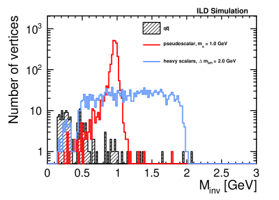
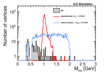
Figure 5: Distributions of the invariant mass of tracks coming out of a displaced vertex, assuming tracks are electrons (left) and pions (right). Black histograms corresponds to q$\bar{\mathrm{q}}$ sample and different colors to various signal scenarios – pseduoscalar with $m_{a}=1$ GeV (red) and scalars with $\Delta m_{AH}=2$ GeV (azure).

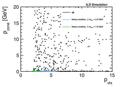
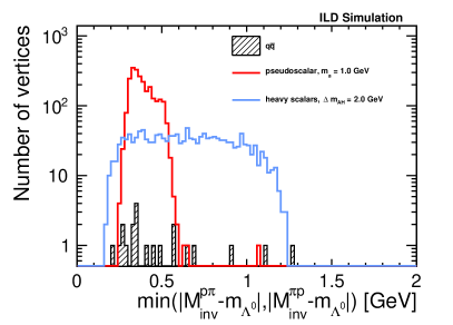
Figure 6: Left: momentum $p_{vtx}$ of the track pair system at a displaced vertex shown as a function of the sum of magnitudes of track momenta, $p_{cone}$, in a cone surrounding the total momentum of track pair coming out of the vertex. Black dots correspond to the q$\bar{\mathrm{q}}$ background, green to scalars with $\Delta m_{AH}=1$ GeV and azure to scalars with $\Delta m_{AH}=2$ GeV. Right: distribution of a difference between $m_{\Lambda^{0}}$ and invariant mass of a track pair assuming that one of them is a pion and the other is a proton, where the smaller of two possible values is taken. Black histogram correspond to the q$\bar{\mathrm{q}}$ background, red to pseduoscalar with $m_{a}=1$ GeV and azure to scalars with $\Delta m_{AH}=2$ GeV.

Table 3: The vertex finding rates directly obtained for the high-$p_{T}$ SM backgrounds inside the TPC region after different sets of cuts. Large statistical uncertainties for tight selection rates result from small number of MC events remaining after the selection. The total number, $N_{bg}$, of background events expected after both selections, taking into account all channels presented in Table 2, is also shown in the last column. $N_{bg}$ is calculated assuming the total luminosity of 2 ab^-1 (for details, see Sec. 6).

background channel	qq	qqqq	$\gamma^{B/W}\gamma^{B/W}$	$N_{bg}$
Finding rate (standard)	$(7.99\pm 0.68)\cdot 10^{-4}$	$(1.486\pm 0.094)\cdot 10^{-3}$	$(2.13\pm 0.28)\cdot 10^{-5}$	128,804
Finding rate (tight)	$(2.30\pm 1.15)\cdot 10^{-5}$	$(3.57\pm 1.46)\cdot 10^{-5}$	$(1.06\pm 0.61)\cdot 10^{-6}$	3,763

5 Vertex finding results

The resulting vertex finding efficiency after selection described in the previous sections, as a function of the true LLP decay vertex radius and $z$ coordinate, is shown in Figure 7 (left) for the $\Delta m_{AH}=2$ GeV heavy scalar scenario. The vertex is considered “correct” if it is reconstructed within 30 mm of the true vertex. In Figure 7 (right) the efficiency is presented as a function of the true decay vertex radius for all the heavy scalar scenarios considered. For the plots presented, cuts on the vertex position were not applied, to indicate differences between the efficiency for LLP decays inside the TPC region and the silicon tracker ($R<329$ mm). It is noticeable that for soft final states the vertex finding efficiency is higher within the TPC volume than in the silicon tracker, which is a direct consequence of a higher track reconstruction efficiency for highly displaced soft tracks [37].

The corresponding vertex finding results for light pseudoscalar production are presented in Figure 8, for the $m_{a}=1$ GeV scenario (left), and compared for all the benchmarks considered (right). Here, in contrary to the heavy scalar case, for the low-mass scenarios the efficiency is higher in the region of silicon detectors (vertex detector, VTX, and silicon internal tracker, SIT), closer to the beam pipe. This is due to very high collinearity of tracks from the LLP decay; in the TPC, hits close to the decay vertex merge, while in a silicon tracker higher resolution allows for a better track separation and more accurate vertex reconstruction. However, it should be noted, that the TPC still greatly enhances the detector acceptance, since in an all-silicon tracker the reconstruction is limited by a number of layers, regardless of the final state kinematics. The dip in efficiency visible in the central part of the detector is an effect of the cuts on $\phi_{1}/\phi_{arc}$ for $z_{12}<100$ mm. If hits close to the vertex merge, one of the tracks has a starting point somewhere along the second track, which looks like those two tracks are intersecting, rather than coming out of a single point.

The final vertex finding efficiencies inside the TPC, after both standard and tight sets of cuts, for the considered scalar and pseudoscalar production scenarios, are presented in Table 4. For the scalars, the efficiency strongly depends on their mass splitting (Z^∗ virtuality), which is responsible for the final state boost. Good performance is achieved for $\Delta m_{AH}\geq 2$ GeV, while for the $\Delta m_{AH}=1$ GeV scenario it suffers mostly from the $p_{T}^{vtx}>1.9$ GeV cut used to suppress the overlay background. For the light pseudoscalars the efficiency dependence is opposite, i.e. it decreases with the final state boost. This is due to the high collinearity of tracks coming from decays of very light particles, the reconstruction of which is more efficient in the silicon detectors (VTX and SIT) because of their better two-hit separation. High performance was obtained for $m_{a}=1$ GeV and larger masses; the results for the $m_{a}=300$ MeV benchmark are limited by the cuts used to suppress background from semileptonic K⁰ decays and misreconstructed photon conversions. It is important to note that the sensitivity in both $\Delta m_{AH}=1$ GeV and $m_{a}=300$ MeV scenarios could be significantly enhanced by a dedicated, model-dependent approach, using additional information about the missing energy or the hard photon produced in association with an ALP.

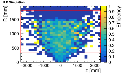
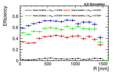
Figure 7: Vertex finding efficiency in the scalar pair-production scenario after the standard selection, but without the cut on the vertex radius. Left: the efficiency as a function of the true LLP decay vertex position in the detector for $\Delta m_{AH}=2$ GeV; the TPC volume is shown with the red box. Right: the efficiency as a function of the true LLP decay vertex radius for all scenarios considered in the analysis.

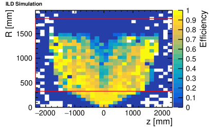
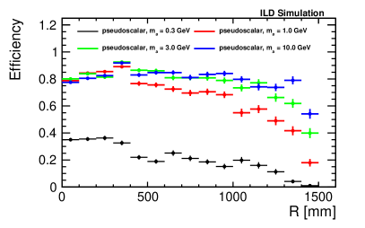
Figure 8: Vertex finding efficiency in the light pseudoscalar production scenario after the standard selection, but without the cut on the vertex radius. Left: the efficiency as a function of the true LLP decay vertex position in the detector for $m_{a}=1$ GeV; the TPC volume is shown with the red box. Right: the efficiency as a function of the true LLP decay vertex radius for all scenarios considered in the analysis.

Table 4: The vertex finding efficiency inside the TPC region obtained in the analysis after different sets of cuts, both for scalars pair-production and light pseudoscalars for all considered scenarios.

$\Delta m_{AH}$ [GeV]	1	2	3	5
Efficiency (standard) [%]	3	33.2	43.4	51.1
Efficiency (tight) [%]	0.4	28.3	40.7	50.2
$m_{a}$ [GeV]	0.3	1	3	10
Efficiency (standard) [%]	7.4	48.4	61.7	65.8
Efficiency (tight) [%]	–	47.3	61.7	65.8

6 Limits on the LLP production cross section

Based on the obtained signal reconstruction efficiencies and expected background levels, the 95% C.L. limits on the signal production cross section are calculated. We assumed the total integrated luminosity of 2 ab^-1 collected in 10 years, with a relative share per beam helicity specified in the ILC H20 scenario [30]. The number of BXs per year is approximately $4.14\cdot 10^{11}$. With 1.55 hadronic overlay events per BX on average, and incoherent e⁺e^- pairs overlay in each BX (for details see Sec. 3), that gives the total estimated number of $1.06\cdot 10^{12}$ of the overlay events. We also use the luminosity for the hard $\gamma^{B}\gamma^{B}$ ($\gamma^{B}\gamma^{W},\gamma^{W}\gamma^{B}$) interactions of $43\%$ (53%) of the total integrated e⁺e^- luminosity [51]. The final number $N_{bg}$ of overlay and hard SM background events remaining after standard selection is 665 and 128,804, respectively, as calculated using the reduction factors obtained in Sections 3 and 4.

To estimate limits for different lifetimes without generating new samples and processing them, signal event re-weighting is performed in order to estimate the limits for a set of LLP lifetimes for every benchmark scenario. For any given mean lifetime $\tau^{\prime}$, an event with LLP decay after a time $t_{i}$ is re-weighted by a ratio $w_{i}=P(t_{i},\tau^{\prime})/P(t_{i},\tau_{0})$ of probabilities $P$ from the exponential distribution, where the mean lifetime $\tau_{0}$ was used to generate an event sample. With the number $N_{p}$ of events containing vertices that match to the MC vertex and pass through the selection, a fraction $\epsilon_{sel}=N_{p}/N_{\text{total}}$ must be calculated to obtain the limit. However, for a very long $\tau^{\prime}$ considered, $c\tau^{\prime}\gg$ 1 m, the number of decays with a large decay length $ct_{i}\sim{\cal O}(c\tau^{\prime})$ in a generated sample can be much smaller than the expected number of these events, leading to large event weights and statistical uncertainties. Therefore, we define a cutoff distance $L_{max}=3$ m, above which finding a vertex is impossible. Then, with $w_{max}$ being the total probability that an LLP decays before $L_{max}$ (calculated from the exponential distribution for a given $\tau^{\prime}$), $N_{\text{total}}=\Sigma_{i}w_{i}/w_{max}$, where only events with LLP decays before $L_{max}$ are considered, and $N_{p}=\Sigma_{i}w_{i}$, where selection cuts are also applied.

The 95% C.L. limit $\sigma_{95\%\mathrm{C.L.}}$ corresponds to the number $N_{lim}=1.96\sqrt{N_{bg}}/\epsilon_{sel}$, where the factor 1.96 corresponds to the unified frequentist interval [52] for the measured number of events equal to the nominal expectation (which is equivalent to the CLs method), assuming $\epsilon_{sel}N_{lim}\ll N_{bg}$ and the Gaussian distribution for the background uncertainty. The limits for each of the considered benchmarks in the scalar pair-production (left) and the light pseudoscalar production (right) scenarios are presented in Figure 9. A range of mean decay lengths $c\tau$ is considered and two sets of limits are presented – for the standard and the tight selection.

In the case of scalar pair-production, good sensitivity can be observed in 0.3-10 m range for $\Delta m_{AH}\geq 2$ GeV. This can be extended by the tight selection, which allows to improve the limits by an order of magnitude. For the $\Delta m_{AH}=1$ GeV scenario, the limits get slightly worsened by the tight selection and go down to the level of tens of femtobarns in the 0.3-3 m range.

For the light pseudoscalars, limits at the order of femtobarns can be obtained with the standard selection for $m_{a}\geq 1$ GeV in a 3-1000 mm range, depending on a scenario. Tight selection improves the limit by even an order of magnitude, allowing to reach the level of femtobarns (or lower) even up to $c\tau\simeq 10$ m. However, it causes a complete loss of sensitivity to the $m_{a}=300$ MeV benchmark, which can be constrained down to $\mathcal{O}$(10 fb) level using the standard selection.

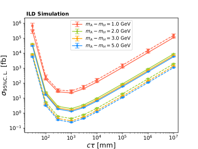
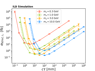
Figure 9: Expected 95% C.L. upper limits on the signal production cross-section for the considered benchmarks and different LLP mean decay lengths, for the scalar pair-production (left) and the light pseudoscalar production (right) at $\sqrt{s}=250$ GeV. Solid lines corresponds to the standard selection and dashed lines to the tight set of cuts. The uncertainties are statistical.

7 Conclusions

We demonstrate the potential of the ILD experiment to search for neutral LLP production, using a displaced vertex signature. The study is based on full detector simulation and conducted from the experimental perspective, with two types of benchmarks. First involves a scalar pair-production, where one of the scalars is long-lived and decays to SM particles and DM. The LLP mass is set to 75 GeV and the mass splitting between the LLP and DM is chosen to be at the $\mathcal{O}$(1 GeV) level, resulting in soft, non-pointing tracks in the final state. The second benchmark type is a production of a very light pseudoscalar with an $\mathcal{O}$(1 GeV) mass, that decays into highly boosted, almost colinear SM particles. Such a choice of benchmarks, that are not fully examined at the LHC, tests the detector performance and reconstruction techniques in very challenging conditions. For each signature, we select four signal scenarios, which are motivated by experimental and kinematic properties, rather than by existing constraints in the parameter space of a specific model.

A number of background processes is considered, both from the beam-beam interactions at a linear collider and hard e⁺e^- scattering. We find a set of cuts, that allow to suppress overwhelming background from the beam-beam events and other SM processes, keeping the model-independent approach. In addition, a tight selection is also proposed to improve the background rejection, slightly reducing the generality of the approach, but improving the sensitivity for most of the signal scenarios considered in the analysis. Finally, based on these selections, we set expected 95% C.L. limits on the signal production cross section. For the pair production of scalars, high reach is observed in 0.3-10 m range from mass splittings of 2 GeV between the LLP and the DM. Good sensitivity can also be reached for pseudoscalar masses from 1 GeV, for mean decay lengths in 0.003-1 m range, depending on LLP mass.

The results presented should be considered the most conservative ones. For specific model scenarios, stronger limits (for smaller masses and mass splittings in particular) could be obtained by exploiting the expected final state topology and kinematic constraints of the model. This is, however, beyond the scope of this paper.

References

- [1] S. L. Glashow “Partial Symmetries of Weak Interactions” In Nucl. Phys. 22, 1961, pp. 579–588 DOI: 10.1016/0029-5582(61)90469-2
- [2] Steven Weinberg “A Model of Leptons” In Phys. Rev. Lett. 19, 1967, pp. 1264–1266 DOI: 10.1103/PhysRevLett.19.1264
- [3] Abdus Salam and John Clive Ward “Weak and electromagnetic interactions” In Nuovo Cim. 11, 1959, pp. 568–577 DOI: 10.1007/BF02726525
- [4] F. Englert and R. Brout “Broken Symmetry and the Mass of Gauge Vector Mesons” In Phys. Rev. Lett. 13, 1964, pp. 321–323 DOI: 10.1103/PhysRevLett.13.321
- [5] Peter W. Higgs “Broken Symmetries and the Masses of Gauge Bosons” In Phys. Rev. Lett. 13, 1964, pp. 508–509 DOI: 10.1103/PhysRevLett.13.508
- [6] G. S. Guralnik, C. R. Hagen and T. W. B. Kibble “Global Conservation Laws and Massless Particles” In Phys. Rev. Lett. 13, 1964, pp. 585–587 DOI: 10.1103/PhysRevLett.13.585
- [7] G. Arnison “Experimental Observation of Isolated Large Transverse Energy Electrons with Associated Missing Energy at GeV” In Phys. Lett. B 122, 1983, pp. 103–116 DOI: 10.1016/0370-2693(83)91177-2
- [8] M. Banner “Observation of Single Isolated Electrons of High Transverse Momentum in Events with Missing Transverse Energy at the CERN anti-p p Collider” In Phys. Lett. B 122, 1983, pp. 476–485 DOI: 10.1016/0370-2693(83)91605-2
- [9] G. Arnison “Experimental Observation of Lepton Pairs of Invariant Mass Around 95-GeV/c**2 at the CERN SPS Collider” In Phys. Lett. B 126, 1983, pp. 398–410 DOI: 10.1016/0370-2693(83)90188-0
- [10] P. Bagnaia “Evidence for at the CERN Collider” In Phys. Lett. B 129, 1983, pp. 130–140 DOI: 10.1016/0370-2693(83)90744-X
- [11] Georges Aad “Observation of a new particle in the search for the Standard Model Higgs boson with the ATLAS detector at the LHC” In Phys. Lett. B 716, 2012, pp. 1–29 DOI: 10.1016/j.physletb.2012.08.020
- [12] Serguei Chatrchyan “Observation of a New Boson at a Mass of 125 GeV with the CMS Experiment at the LHC” In Phys. Lett. B 716, 2012, pp. 30–61 DOI: 10.1016/j.physletb.2012.08.021
- [13] R. Barbier “R-parity violating supersymmetry” In Phys. Rept. 420, 2005, pp. 1–202 DOI: 10.1016/j.physrep.2005.08.006
- [14] Matthew J. Strassler and Kathryn M. Zurek “Echoes of a hidden valley at hadron colliders” In Phys. Lett. B 651, 2007, pp. 374–379 DOI: 10.1016/j.physletb.2007.06.055
- [15] David E. Kaplan, Markus A. Luty and Kathryn M. Zurek “Asymmetric Dark Matter” In Phys. Rev. D 79, 2009, pp. 115016 DOI: 10.1103/PhysRevD.79.115016
- [16] Eder Izaguirre, Gordan Krnjaic and Brian Shuve “Discovering Inelastic Thermal-Relic Dark Matter at Colliders” In Phys. Rev. D 93.6, 2016, pp. 063523 DOI: 10.1103/PhysRevD.93.063523
- [17] Martin Bauer, Matthias Neubert and Andrea Thamm “Collider Probes of Axion-Like Particles” In JHEP 12, 2017, pp. 044 DOI: 10.1007/JHEP12(2017)044
- [18] Juliette Alimena “Searching for long-lived particles beyond the Standard Model at the Large Hadron Collider” In J. Phys. G 47.9, 2020, pp. 090501 DOI: 10.1088/1361-6471/ab4574
- [19] Aram Hayrapetyan “Search for long-lived particles decaying in the CMS muon detectors in proton-proton collisions at = 13 TeV”, 2024 arXiv:2402.01898 [hep-ex]
- [20] Morad Aaboud “Search for long-lived particles produced in collisions at TeV that decay into displaced hadronic jets in the ATLAS muon spectrometer” In Phys. Rev. D 99.5, 2019, pp. 052005 DOI: 10.1103/PhysRevD.99.052005
- [21] A. M. Sirunyan “Search for decays of stopped exotic long-lived particles produced in proton-proton collisions at 13 TeV” In JHEP 05, 2018, pp. 127 DOI: 10.1007/JHEP05(2018)127
- [22] Albert M Sirunyan “Search for long-lived particles using displaced jets in proton-proton collisions at 13 TeV” In Phys. Rev. D 104.1, 2021, pp. 012015 DOI: 10.1103/PhysRevD.104.012015
- [23] Aram Hayrapetyan “Search for long-lived particles using displaced vertices and missing transverse momentum in proton-proton collisions at = 13 TeV”, 2024 arXiv:2402.15804 [hep-ex]
- [24] Morad Aaboud “Search for long-lived, massive particles in events with displaced vertices and missing transverse momentum in = 13 TeV collisions with the ATLAS detector” In Phys. Rev. D 97.5, 2018, pp. 052012 DOI: 10.1103/PhysRevD.97.052012
- [25] Georges Aad “Search for light long-lived neutral particles from Higgs boson decays via vector-boson-fusion production from collisions at TeV with the ATLAS detector”, 2023 arXiv:2311.18298 [hep-ex]
- [26] Aram Hayrapetyan “Search for long-lived particles decaying to final states with a pair of muons in proton-proton collisions at = 13.6 TeV”, 2024 arXiv:2402.14491 [hep-ex]
- [27] Lawrence Lee “Collider Searches for Long-Lived Particles Beyond the Standard Model” [Erratum: Prog.Part.Nucl.Phys. 122, 103912 (2022)] In Prog. Part. Nucl. Phys. 106, 2019, pp. 210–255 DOI: 10.1016/j.ppnp.2019.02.006
- [28] C. Antel “Feebly-interacting particles: FIPs 2022 Workshop Report” In Eur. Phys. J. C 83.12, 2023, pp. 1122 DOI: 10.1140/epjc/s10052-023-12168-5
- [29] European Strategy Group “2020 Update of the European Strategy for Particle Physics” Geneva: CERN Council, 2020 DOI: 10.17181/ESU2020
- [30] Philip Bambade “The International Linear Collider: A Global Project”, 2019 arXiv:1903.01629
- [31] “A Multi-TeV Linear Collider Based on CLIC Technology: CLIC Conceptual Design Report”, 2012 DOI: 10.5170/CERN-2012-007
- [32] A. Abada “FCC-ee: The Lepton Collider: Future Circular Collider Conceptual Design Report Volume 2” In Eur. Phys. J. ST 228.2, 2019, pp. 261–623 DOI: 10.1140/epjst/e2019-900045-4
- [33] “CEPC Conceptual Design Report: Volume 1 - Accelerator”, 2018 arXiv:1809.00285 [physics.acc-ph]
- [34] “The International Linear Collider Technical Design Report - Volume 2: Physics”, 2013 arXiv:1306.6352 [hep-ph]
- [35] Jorge Blas “Focus topics for the ECFA study on Higgs / Top / EW factories”, 2024 arXiv:2401.07564 [hep-ph]
- [36] Halina Abramowicz “International Large Detector: Interim Design Report”, 2020 arXiv:2003.01116
- [37] Jan Klamka “Reconstructing long-lived particles with the ILD detector” In PoS EPS-HEP2023, 2024, pp. 458 DOI: 10.22323/1.449.0458
- [38] M.A. Thomson “Particle flow calorimetry and the PandoraPFA algorithm” In Nuclear Instruments and Methods in Physics Research Section A: Accelerators, Spectrometers, Detectors and Associated Equipment 611.1 Elsevier BV, 2009, pp. 25–40 DOI: 10.1016/j.nima.2009.09.009
- [39] Jan Kalinowski “Benchmarking the Inert Doublet Model for colliders” In JHEP 12, 2018, pp. 081 DOI: 10.1007/JHEP12(2018)081
- [40] Ruth Schäfer “Near or far detectors? A case study for long-lived particle searches at electron-positron colliders” In Phys. Rev. D 107.7, 2023, pp. 076022 DOI: 10.1103/PhysRevD.107.076022
- [41] Wolfgang Kilian “WHIZARD: Simulating Multi-Particle Processes at LHC and ILC” In Eur. Phys. J. C 71, 2011, pp. 1742 DOI: 10.1140/epjc/s10052-011-1742-y
- [42] M Frank, F Gaede, C Grefe and P Mato “DD4hep: A Detector Description Toolkit for High Energy Physics Experiments” In Journal of Physics: Conference Series 513.2 IOP Publishing, 2014, pp. 022010 DOI: 10.1088/1742-6596/513/2/022010
- [43] S. Agostinelli “Geant4 — a simulation toolkit” In Nucl. Instrum. Meth. A 506.3, 2003, pp. 250 –303 DOI: https://doi.org/10.1016/S0168-9002(03)01368-8
- [44] C Grefe, S Poss, A Sailer and A Tsaregorodtsev “ILCDIRAC, a DIRAC extension for the Linear Collider community” In J. Phys.: Conf. Ser. 513.CLICdp-Conf-2013-003, 2013, pp. 032077. 5 URL: https://cds.cern.ch/record/1626585
- [45] “iLCSoft – Linear Collider Software” In GitHub repository GitHub, https://github.com/iLCSoft
- [46] F. Gaede “Marlin and LCCD: Software tools for the ILC” In Nucl. Instrum. Meth. A 559, 2006, pp. 177–180 DOI: 10.1016/j.nima.2005.11.138
- [47] “ILDConfig” In GitHub repository GitHub, https://github.com/iLCSoft/ILDConfig/tree/master/StandardConfig/production
- [48] Thomas Kramer “Track parameters in LCIO”, 2006
- [49] Frank Gaede et al. “Track reconstruction at the ILC: the ILD tracking software” In Journal of Physics: Conference Series 513.2, 2014, pp. 022011 DOI: 10.1088/1742-6596/513/2/022011
- [50] D. Schulte “Beam-beam simulations with GUINEA-PIG”, 1999
- [51] Mikael Berggren, private communication
- [52] Gary J. Feldman and Robert D. Cousins “A Unified approach to the classical statistical analysis of small signals” In Phys. Rev. D 57, 1998, pp. 3873–3889 DOI: 10.1103/PhysRevD.57.3873