Properties of non-cryogenic DTs and their relevance for fusion

Abstract

In inertial confinement fusion, pure deuterium-tritium (DT) is usually used as a fusion fuel. In their paper [1], Guskov et al. instead propose using low-Z compounds that contain DT and are non-cryogenic at room temperature. They suggest that these fuels (here called non-cryogenic DTs) can be ignited for $\rho_{\ce{DT}}R\geq 0.35\,\ce{g}\,\ce{cm^{-2}}$ and $kT_{\ce{e}}\geq 14\,\ce{keV}$, i.e., parameters which are more stringent but still in the same order of magnitude as those for DT. In deriving these results the authors in [1] assume that ionic and electronic temperatures are equal and consider only electronic stopping power. Here, we show that at temperatures greater than 10 keV, ionic stopping power is not negligible compared to the electronic one. We demonstrate that this necessarily leads to higher ionic than electronic temperatures. Both factors facilitate ignition compared to the model used in [1] showing that non-cryogenic DT compounds are more versatile than previously known. In addition, we find that heavy beryllium borohydride ignites more easily than heavy beryllium hydride, the best-performing fuel found by Guskov et al. Our results are based on an analytical model that incorporates a detailed stopping power analysis, as well as on numerical simulations using an improved version of the community hydro code MULTI-IFE. Alleviating the constraints and costs of cryogenic technology and the fact that non-cryogenic DT fuels are solids at room temperature open up new design options for fusion targets with $Q>100$ and thus contribute to the larger goal of making inertial fusion energy an economically viable source of clean energy. In addition, the discussion presented here generalizes the analysis of fuels for energy production.

contents=

1 Introduction

In search of fusion fuels which are solids at room temperature, we have recently started to investigate a class of non-cryogenic chemical compounds in [2, 3, 4, 5]. They consist of elements with charge numbers $Z$ of 1 to 5 which bind hydrogen in solid form. As deuterium and tritium have chemically almost identical properties as hydrogen, we assume that it is possible to replace the hydrogen atoms by deuterium and tritium in equal ratios. We call the resulting compounds non-cryogenic DTs.

In [2, 3, 4, 5] the focus has been on non-igniting inertial fusion energy (IFE) targets with gain $G\approx 1$ without fuel pre-compression preheated with only a few $\ce{MJ}$ to highlight the interesting properties of non-cryogenic DTs. However, as is widely accepted, high gain $G\gg 1$ in IFE on a practical level rests on at least two points: I) The fuels must be capable of igniting and II) fuel compression is needed to reduce the fuel mass to a level acceptable for ignition and energy production. The present paper focuses on the first of these aspects and studies several practical compounds in greater depth beyond the more academic fuels initially addressed in [2, 3, 4, 5].

Non-cryogenic DTs are compounds with an inactive low-Z and an active DT component. Their total mass density is given by $\rho=\rho_{\ce{Z}}+\rho_{\ce{DT}}$, where $\rho_{\ce{Z}}$ denotes the low-Z and $\rho_{\ce{DT}}$ the $\ce{DT}$ mass density. Table 1 provides a non-exhaustive list of non-cryogenic DT compounds which, as we show, can ignite, reach high fusion gain and thus serve as potential fusion fuels. They are chosen for their high mass density of $\ce{DT}$ relative to the mass density of the low-$Z$ elements. In fact, their $\ce{DT}$ density is higher than the one of $\ce{DT}$ ice.

The fuel compounds we consider should be distinguished from so-called contaminated fuels, see e.g. [6, 7]. In our case, the presence of $Z>1$ ions is essential for the properties of the fuel, combining the downside of increased radiation losses with significant upsides like the fuel being a solid material at room temperature and having increased stopping power, whereas for contaminated fuels the presence of $Z>1$ is usually unwanted.

Non-cryogenic chemical compounds with inactive impurities and active $\ce{DT}$ for fusion applications have previously been addressed by Guskov et al. [1, 8, 9, 10]. The authors call these compounds low-Z fuels and find that they are capable of igniting and of producing gain (see [1, table 2]) assuming equal electron and ion temperatures $kT_{\ce{e}}=kT_{\ce{i}}=kT$. The authors assume that stopping of the fusion $\alpha$-particles is only due to electrons. However, as we show here, ionic fuel temperatures can be considerably higher than the electronic one, implying $kT_{\ce{i}}>kT_{\ce{e}}$. Moreover, ionic $\alpha$-particle stopping becomes relevant in non-cryogenic DT at its elevated ignition temperatures. Including these effects, we improve the versatility of low-Z fuels beyond the predictions made in [1, 9] since the effective fusion power grows relative to the power loss by radiation for $kT_{\ce{i}}>kT_{\ce{e}}$. What is more, the chemical compound that performs best in this study, heavy beryllium borohydride, needs about $10\%$ lower confinement parameter $\rho_{\mathrm{DT}}R$ to be ignited compared to heavy beryllium hydride, the compound advocated for in [1, 9]. It also requires about $10\%$ lower ignition energy due to a lower number of electrons and ions per pair of deuterium and tritium ions.

The paper is structured as follows. In sec. 2 we introduce our analytical model for ignition for the ideal case of a pre-compressed static plasma and neglecting fuel consumption. This includes a novel analysis of ionic and electronic stopping powers for $\alpha$-particles and neutronic energy deposition in the fuel. Importantly, these simplifications allow for a temperature flow analysis in a static geometry, enabling us to identify a quasi-equilibrium of ion and electron temperatures with $kT_{i}>kT_{e}$. Using this analysis, we identify the minimal confinement parameters $\rho_{\ce{DT}}\,R$ for ignition as well as the corresponding ignition temperatures for the selected non-cryogenic DT compounds. Moreover, we contrast the energy deposition to ions and electrons for non-cryogenic DT fuels with that for DT. In sec. 3, we compare this analytical model with numerical simulations using an improved version of the MULTI-IFE hydro code for a pre-compressed, static plasma considering fuel consumption. In sec. 4 we make the MULTI-IFE predictions plausible with the help of simple analytical considerations. We conclude in sec. 5. While the main text is kept brief, theoretical derivations and technical details are included in dedicated appendices.

name	composition	$\rho$	$\rho_{\ce{DT}}$
deuterium-tritium	DT	0.225	0.225
beryllium borohydride	$\ce{Be}[\ce{BD}_{2}\ce{T}_{2}]_{2}$	0.790	0.310
beryllium hydride	BeDT	0.961	0.343
lithium borohydride	$\ce{LiBD}_{2}\ce{T}_{2}$	0.848	0.303

Table 1: Non-cryogenic DT compounds, their total mass densities $\rho=\rho_{\ce{Z}}+\rho_{\ce{DT}}$ and their $\ce{DT}$ mass densities $\rho_{\ce{DT}}$ bound in the compound. The mass densities have been calculated from chemical tables [11, 12, 13, 14] by exchanging hydrogen by deuterium and tritium. The mass densities of $\ce{BeDT}$ have been obtained using the crystalline state density of $\ce{BeH_{2}}$. All densities are in units of $\ce{g}\,\ce{cm^{-3}}$.

2 Analytical model for ignition

Overview of the model

Ignition is the rise of temperatures due to the fusion power deposited to the plasma exceeding the combined power losses. Here we consider the power balance for a spherical fusion plasma with confinement parameter $\rho_{\ce{DT}}R$ as can be reached in the stagnation phase of fuel pre-compression. We include radiation losses by bremsstrahlung $Q_{\text{rad}}$ given by (7), losses due to escaping $\alpha$-particles at the surface by making use of the deposition powers $Q_{\ce{fus\rightarrow i}}$ given by (12) and $Q_{\ce{fus\rightarrow e}}$ given by (12), electronic heat loss at the surface $Q_{\ce{e}}$ given by (8), and heat transfer $Q_{\ce{bc}}$ between the different particle species in the plasma given by (11) (see A.1). The deposition powers to ions $Q_{\mathrm{fus}\rightarrow i}$ and electrons $Q_{\mathrm{fus}\rightarrow e}$ are calculated in detail according to a novel stopping power model for alpha particles and neutrons, making use of the Euler equations (15)–(17) for spherical geometry (see A). We neglect hydro motion as well as fuel depletion. Importantly, these simplifications allow for a temperature flow analysis in an otherwise static situation. To justify the application of this analysis to a fusion scheme, one needs to assume that the stagnation phase is sufficiently long for ignition to happen and that fuel depletion is not too severe. To include fuel depletion and to cross-check the model, we perform one-dimensional MULTI-IFE simulations neglecting hydro motion in sec. 3.

With the help of (15)–(17) derived from (A.2) via an eight moments ansatz, neglecting hydro motion, and integration over a finite spherical volume, the following temperature flow model can be derived:

$$\frac{3}{2}n_{i}\frac{\partial kT_{i}}{\partial t} =\sum_{\ell}Q_{i\ell}+Q_{\ce{fus\rightarrow i}}\,,$$ (1)

$$\frac{3}{2}n_{e}\frac{\partial kT_{e}}{\partial t} =\sum_{\ell}Q_{e\ell}+Q_{\ce{fus\rightarrow e}}-Q_{\text{rad}}-Q_{e}\,,$$ (2)

where the index $i$ refers to different ion species, $e$ to electrons, $n$ to particle densities, and $kT$ to temperatures. Volume integration leads to boundaries at which radiation, electronic heat loss, $\alpha$-particle, and neutron losses can occur. The power densities $Q_{\ce{fus\rightarrow i}}$ and $Q_{\ce{fus\rightarrow e}}$ are fusion power densities obtained by considering the fusion energy deposition due to $\alpha$-particle stopping as discussed in A.2, due to $\alpha$-particle loss as discussed in A.3, neutron energy deposition due to elastic scattering as discussed in A.4, and due to neutron loss at the boundaries. As we shall show, a significant fraction of the $\alpha$-particle energy directly heats the ions in non-cryogenic DT at the required ignition temperatures $kT_{\ce{e}}$. Moreover, the fusion neutrons pass non-negligible fractions of their energy directly to the $\ce{DT}$-ions through elastic scattering.

Ignition diagrams

Numerically solving (1) and (2) for different initial temperatures yields the temperature flow diagram in Fig. 1, here shown for heavy beryllium borohydride at $\rho_{\mathrm{DT}}R=0.5\,\mathrm{g}\,\mathrm{cm}^{-2}$ (top) and $\rho_{\mathrm{DT}}R=1.0\,\mathrm{g}\,\mathrm{cm}^{-2}$ (bottom). For illustrative purposes, we represent the flow in the plane of the electron temperature $kT_{e}$ and the average ion temperature $\langle kT_{\ce{i}}\rangle=\sum_{i}n_{i}kT_{\ce{i}}/\sum_{i}n_{\ce{i}}$. The temperature flows are obtained by plotting the flow directions obtained from two consecutive numerical temperature values.

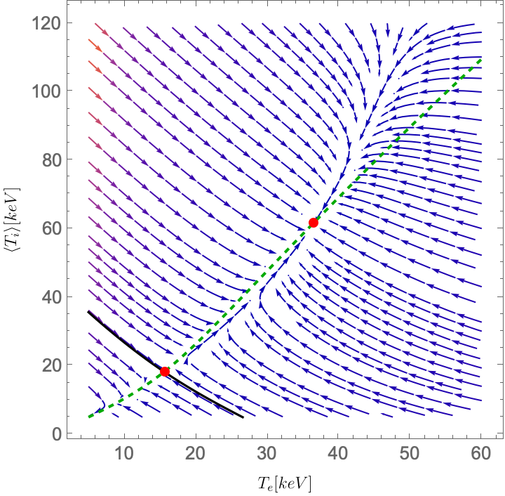
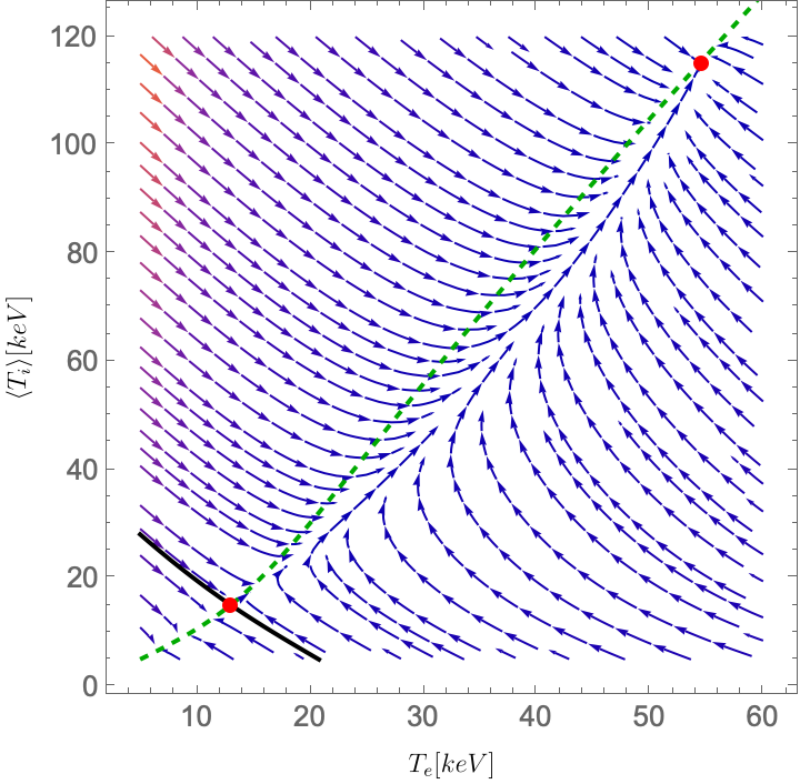
Figure 1: Temperature flow diagrams for $\ce{Be[BD_{2}T_{2}]_{2}}$ at $\rho_{\ce{DT}}R=0.5\,\ce{g}\,\ce{cm^{-2}}$ (top) and $\rho_{\ce{DT}}R=1.0\,\ce{g}\,\ce{cm^{-2}}$ (bottom), where $\rho_{\ce{DT}}=50\,\ce{g}\,\ce{cm^{-3}}$, $R=0.01\,\ce{cm}$, and $R=0.02\,\ce{cm}$. The plots illustrate the flow of the electron temperature $kT_{\ce{e}}$ and the averaged ion temperature $\langle kT_{\ce{i}}\rangle$ according to Eqs. (1) and (2). The important findings are (i) $\left\langle kT_{\ce{i}}\right\rangle>kT_{\ce{e}}$ on the central line and (ii) that ignition happens if the systems are started in the regions above the solid black lines in both plots. Temperatures higher than those at the upper red dots cannot be stably reached according to the model. According to Fig. 2 and the present figure, higher values of $\rho_{\ce{DT}}R$ lower the ignition temperatures and increase the peak temperatures the system can reach. For the case of $\rho_{\ce{DT}}R=0.5\,\ce{gcm^{-2}}$ ignition can occur for $kT_{\ce{e}}\approx 16\,\ce{keV}$ and $kT_{\ce{i}}\approx 20\,\ce{keV}$. For the case of $\rho_{\ce{DT}}R=1.0\,\ce{gcm^{-2}}$ ignition can occur at $kT_{\ce{e}}\approx 14\,\ce{keV}$ and $kT_{\ce{i}}\approx 18\,\ce{keV}$.

The diagram shows that the temperature flow is first attracted to the green central line by fast inter-species power equilibration. Thereafter, the temperature flow follows this central line to one of the fixed points. The central line thus defines a quasi-equilibrium of ion and electron temperatures, i.e, more precisely, a function $kT_{\ce{i}}(kT_{\ce{e}})$ for every ion species $i$. This quasi-equilibrium can be approximately determined by considering the flow of the ionic temperatures for a fixed electron temperature (see the green line in the diagram). Details are given in A.5. As we can see, the quasi-equilibrium is reached for higher ion than electron temperatures, especially at overall higher temperatures. Moreover, as illustrated in Figure 1 two fixed points lie on the quasi-equilibrium line: I) An unstable one at $kT_{e}\approx 13\,\mathrm{keV}$ and $\langle kT_{i}\rangle\approx 15\,\mathrm{keV}$ for $\rho_{\ce{DT}}R=1.0\,\ce{g}\,\ce{cm^{-2}}$ and II) a stable one at $kT_{e}\approx 54\,\mathrm{keV}$ and $\langle kT_{i}\rangle\approx 115\,\mathrm{keV}$ for the same $\rho_{\ce{DT}}R$. For $\rho_{\ce{DT}}R=0.5\,\ce{g}\,\ce{cm^{-2}}$, they move to $kT_{e}\approx 16\,\mathrm{keV}$, $\langle kT_{i}\rangle\approx 18\,\mathrm{keV}$ and $kT_{e}\approx 38\,\mathrm{keV}$, $\langle kT_{i}\rangle\approx 65\,\mathrm{keV}$, respectively.

The stable fixed point is the point of self-sustained fusion burn. It exists because fuel consumption is not considered here. The unstable fixed point is the point in quasi-equilibrium through which the solid black line passes that separates the region of cooling down to zero temperatures from the attraction basin of the stable fixed point. It can also be called the ignition point. However, it is the joint existence of the two fixed points that shows that ignition is possible. When lowering the parameter $\rho_{\ce{DT}}R$ (see Fig. 1 bottom), they move closer together, merge into a single point at which the minimal $\left(\rho_{\ce{DT}}R\right)_{\ce{min}}$ and minimal temperatures $\left(kT_{\ce{e}}\right)_{\ce{min}}$ and $\left(kT_{\ce{i}}\right)_{\ce{min}}$ are reached and finally disappear.

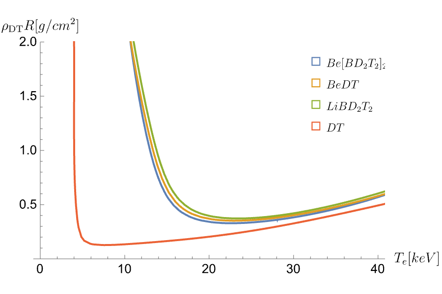
Figure 2: Ignition conditions for $\ce{Be[BD_{2}T_{2}]_{2}}$, $\ce{BeDT}$, $\ce{LiBD_{2}T_{2}}$, and $\ce{DT}$. calculated via the analytical model (1) and (2). Individual temperatures $kT_{\ce{b}}$ for each of the constituents $\ce{b}$ in the fuel have been considered.

compound	$\left(\rho_{\ce{DT}}R\right)_{\ce{min}}$	$\left(kT_{\ce{e}}\right)_{\ce{min}}$
DT	0.13	7
$\ce{Be}[\ce{BD}_{2}\ce{T}_{2}]_{2}$	0.33	22
BeDT	0.35	23
$\ce{LiBD}_{2}\ce{T}_{2}$	0.37	23

Table 2: Minimal confinement parameters $\left(\rho_{\ce{DT}}R\right)_{\ce{min}}$ and corresponding electron temperatures $kT_{\ce{e}}$ required for ignition of non-cryogenic DT compounds as obtained from the analytical model

The minimal ignition parameters can be studied by setting gain and loss terms (see A.1) equal to each other and plotting the resulting ignition curves in the $kT_{\ce{e}}$-$\rho_{\ce{DT}}R$ plane. Here, it is assumed that the ionic species assume the temperatures $kT_{\ce{i}}(kT_{\ce{e}})$ in quasi-equilibrium. The ignition curves separate the regions of cooling down and of ignition. As visible in Fig. 2, they are flat around their minimum, implying that a small increase in $\rho_{\ce{DT}}R$ leads to a significant decrease in the necessary ignition temperature $kT_{\ce{e}}$. The minimal confinement parameters $\left(\rho_{\ce{DT}}R\right)_{\ce{min}}$ and corresponding ignition temperatures $\left(kT_{\ce{e}}\right)_{\ce{min}}$ are listed in Table 2 for the different fuel compounds. We find that among the non-cryogenic DT fuels considered, heavy beryllium borohydride has the lowest value of $\left(\rho_{\ce{DT}}R\right)_{\ce{min}}$, followed by heavy beryllium hydride, the fuel advocated for by Guskov et al. [1].

Figure 3: (Previous page.) Left: Normalized power densities $q=Q/n_{\ce{D}}n_{\ce{T}}$. Comparison of $q_{\alpha}+q_{\ce{n}}$ for $kT_{\ce{e}}$ and $\left\langle kT_{\ce{i}}\right\rangle$ in quasi-equilibrium (solid blue line) and $q_{\alpha}+q_{\ce{n}}$ for $kT_{\ce{e}}=kT_{\ce{i}}$ (dashed blue line) with $q_{\ce{rad}}+q_{\ce{\alpha\rightarrow loss}}+q_{\ce{e}}$, $q_{\ce{rad}}+q_{\ce{\alpha\rightarrow loss}}$, and $q_{\ce{rad}}$ versus $kT_{\ce{e}}$ at $\rho_{\ce{DT}}R=0.5\,\ce{g}\,\ce{cm}^{-2}$, where $q_{\alpha}$ is the normalized fusion power density in $\alpha$ particles, $q_{\ce{n}}$ the normalized deposited fusion power density in neutrons, $q_{\ce{fus\rightarrow loss}}$ the normalized $\alpha$-particle loss, and $q_{\ce{e}}$ the normalized electronic heat conduction loss. Right: Fraction of $\alpha$-particle energy transferred to the individual constituents of the compound and the electrons versus $kT_{\ce{e}}$ at the corresponding ion temperatures $kT_{\ce{i}}$ in quasi-equilibrium.

Role of unequal temperatures for ignition

Ignition of the fuels in Table 2 is possible because of two crucial facts: First, $kT_{\ce{i}}>kT_{\ce{e}}$ facilitates ignition. This is illustrated for $\ce{Be[BD_{2}T_{2}]_{2}}$ at $\rho_{\ce{DT}}R=0.5\,\ce{g}\,\ce{cm}^{-2}$ in Fig. 3 (second row left), where it is shown that for the temperatures $kT_{\ce{i}}>kT_{\ce{e}}$ in the quasi-equilibrium the system adopts the fusion power is significantly greater than at equal temperatures $kT_{\ce{e}}=kT_{\ce{i}}$. In fact, at equal temperatures, the cumulative losses (solid red curve) always exceed the fusion power (dashed blue curve) so that ignition would not be possible at this $\rho_{\ce{DT}}R$. The reason for this behavior is that higher values of $kT_{\ce{i}}$ normally lead to higher fusion power while radiation and electron heat conduction losses increase with $kT_{\ce{e}}$. Second, the ionic $\alpha$-particle stopping power of the fuel compound $\ce{Be[BD_{2}T_{2}]_{2}}$ becomes comparable to the electronic stopping power at the ignition temperature and eventually dominates at even higher temperatures (see Fig. 3 second row right). In this way, the temperature spread between $kT_{\ce{i}}$ and $kT_{\ce{e}}$ is sustained.

We now compare deposition powers to electrons and ions of non-cryogenic DT fuels ($\ce{Be[BD_{2}T_{2}]_{2}}$, $\ce{BeDT}$ and $\ce{LiBD_{2}T_{2}}$) with those of pure DT at $\rho_{\ce{DT}}R=0.5\,\ce{g}\,\ce{cm}^{-2}$ (see Figure 3). For all these fuels and for $kT_{e}<10\,\mathrm{keV}$, most of the $\alpha$-particle energy is deposited into electrons and losses due to $\alpha$-particles escaping the system are small. For $kT_{e}>20\,\mathrm{keV}$, however, these losses increase sharply for $\ce{DT}$ while for $\ce{Be[BD_{2}T_{2}]_{2}}$, $\ce{LiBD_{2}T_{2}}$, and $\ce{BeDT}$, they are largely compensated by the $Z>1$ ions. The reason for this behavior is that the electronic stopping power decreases as $kT_{e}^{-3/2}$ while the ionic one is approximately independent of temperature in this range. A detailed discussion is given in A.2. Consequently, the share of fusion power deposited into electrons decreases with temperature while the share deposited into ions increases. As mentioned above, this is a major reason why the ions can sustain significantly greater temperatures than the electrons. Among the ionic species, most of the fusion power is deposited to the one with the greatest charge number $Z$, since stopping power increases with $Z^{2}$.

Overall, we find that the selected non-cryogenic DT compounds have significantly greater alpha stopping power than DT. This implies that the higher radiation loss of non-cryogenic DT compounds is to a great extent compensated by their enhanced stopping power for $\alpha$-particles (and neutrons), especially for $kT_{\ce{e}}>10\,\ce{keV}$. The temperature spread between $kT_{\ce{i}}$ and $kT_{\ce{e}}$ is present for both DT and non-cryogenic DT compounds and becomes significant for $kT_{\ce{e}}>10\,\ce{keV}$. As this is the temperature range relevant for the ignition of non-cryogenic DT compounds, it has a stronger impact on the possibility of ignition for the latter.

3 Numerical simulations

We now compare our analytical model with the predictions of the freely available numerical hydro code MULTI-IFE, which is well-tested in its original version for pure DT. For non-cryogenic DTs the code requires adaptations which we discuss in B. By simulating cases similar to the ones discussed on the basis of the analytical model, we obtain an approximate cross-check of the results.

In order to create a direct comparison with the temperature flow analysis of (1) and (2), the hydro motion in the code is switched off corresponding to an isobaric scenario. Unlike in the analytical model, fuel consumption and radiation re-absorption are taken into account in the simulations.

Several parametric simulations for a highly compressed spherical $\ce{Be[BD_{2}T_{2}]_{2}}$ plasma at $\langle\rho_{\ce{DT}}\rangle R=0.25\,\ce{g}\,\ce{cm}^{-2}$ with different initial electron and ion temperatures have been performed, yielding the flow trajectories in the $\left(kT_{\ce{e}},kT_{\ce{i}}\right)$-plane shown in Figure 4 (bottom left). The further plots show the fusion gain as a function of $kT_{\ce{e}}$ (top left), the gain as a function of time (top right) and $kT_{\ce{i}}$ as a function of time (bottom right).

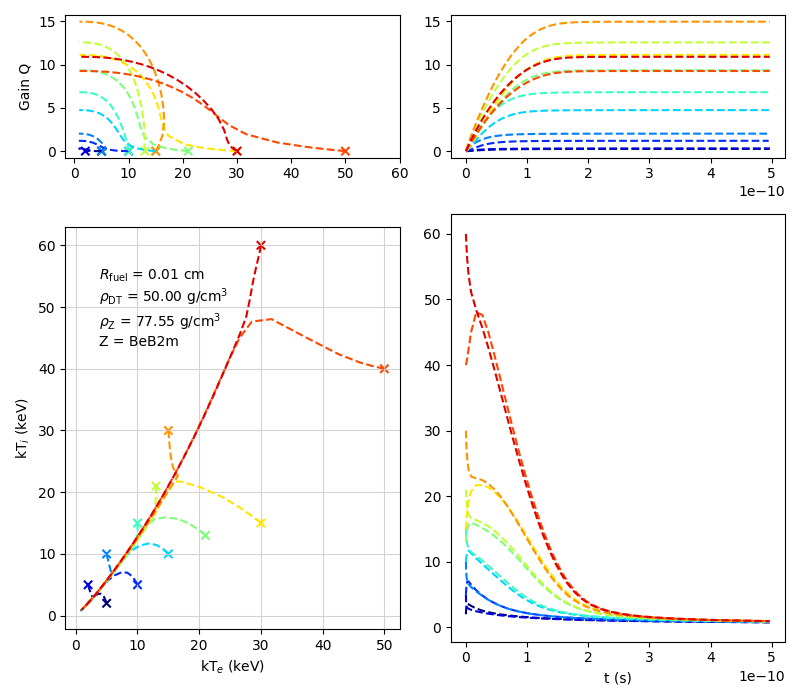
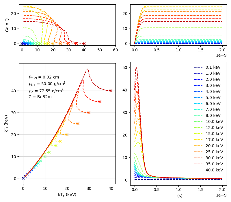
Figure 4: Results of two sets of MULTI-IFE simulations without hydro motion. The left four panels correspond to the case where $R_{\mathrm{fuel}}=0.01$ cm and the right four panels for $R_{\mathrm{fuel}}=0.02$ cm. The material in both simulations is $\ce{Be[BD_{2}T_{2}]_{2}}$ with the density $\rho_{\ce{DT}}=2\langle\rho_{\ce{DT}}\rangle=50\,\ce{g}\,\ce{cm^{-3}}$ in the $\ce{DT}$ cells and different initial electron and ion temperatures. These settings correspond to $\langle\rho_{\ce{DT}}\rangle R=0.25\,\ce{g}\,\ce{cm^{-2}}$ for the left case and $\langle\rho_{\ce{DT}}\rangle R=0.5\,\ce{g}\,\ce{cm^{-2}}$ for the right case since $\ce{DT}$ and $\ce{Z}$ cells alternate. For both cases top left: Gain versus electron temperature. Bottom left: Trajectories in the $\left(kT_{\ce{e}},kT_{\ce{i}}\right)$ plane. Top right: Gain as a function of time. Bottom right: Ion temperature as a function of time. The initial internal energy for the numerical setup corresponding to the orange dashed line in the left plot with $kT_{\ce{e}}\approx 15\,\ce{keV}$ and $kT_{\ce{i}}\approx 30\,\ce{keV}$ is approximately $494\,\ce{kJ}$ and for the orange dashed line in right plot with $kT_{\ce{e}}=kT_{\ce{i}}\approx 20\,\ce{keV}$ it is about $4.02\,\ce{MJ}$. No or only marginal ignition takes place for the left scenario while there is robust ignition for the right one in agreement with Fig. 2.

The numerical results agree qualitatively with the predictions of our analytical model. The simulated temperature flow diagram is similar to the analytical one in Figure 1. The simulations also show that a quasi-equilibrium is reached prior to rising temperatures due to fusion gain. The code predicts $kT_{\ce{i}}>kT_{\ce{e}}$ even slightly more pronounced than in the analytical model.

Below certain initial temperatures, the system does not ignite but cools down to zero temperatures while above them further fuel heating and then cooling sets in. Since the $f$-number (fractional fuel content) drops (see Fig. 5), the cooling is the result of fuel depletion, which contrary to the analytical model precludes the existence of an upper stable fixed point. The turning points of the trajectories and the fusion gain depend on the initial temperatures. The simulations in Fig. 4 suggest that for $\rho_{\ce{DT}}\,R=0.5\,\ce{gcm^{-2}}$ ignition is possible for initial temperatures $kT_{\ce{e}}=kT_{\ce{i}}=15\,\ce{keV}$, which agrees well with those predicted by the analytical model for the same $\rho_{\ce{DT}}\,R$.

Figure 5 complements Fig. 4 for the same parameters and assumptions. The plots show the fusion energy as a function of time (top), the fractional fuel content $f(t)=n_{\ce{D}}(t)/(n_{\ce{D}}(0)+n_{\ce{T}}(0))$ as a function of time (middle) and the fusion power versus time (bottom).

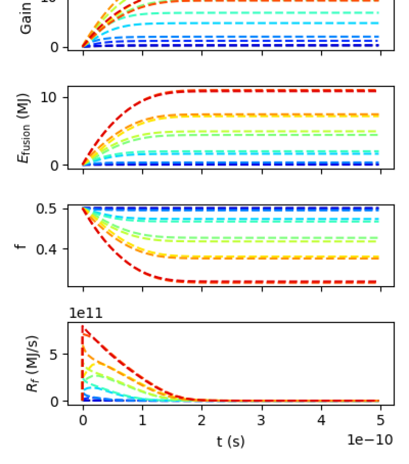
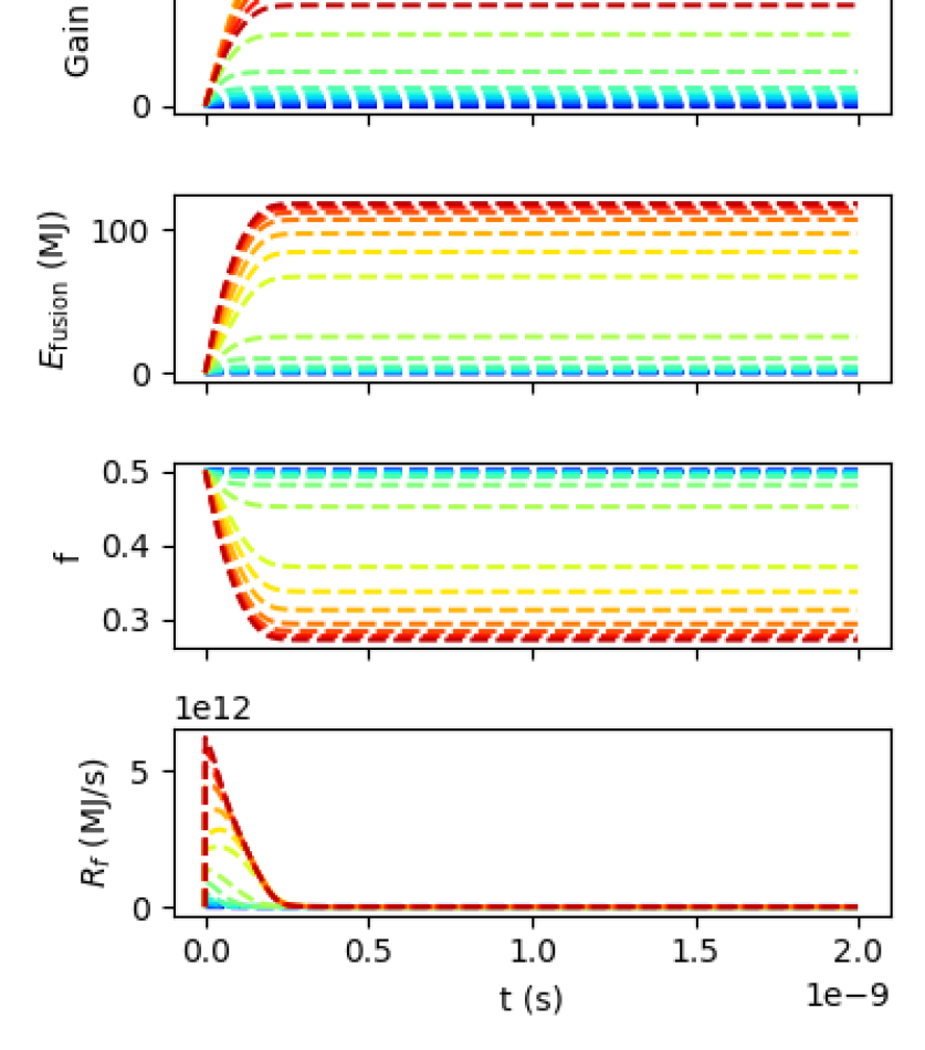
Figure 5: Results of MULTI-IFE simulations of $\ce{Be[BD_{2}T_{2}]_{2}}$ without hydro motion and $\rho_{\ce{DT}}R=0.25\,\ce{g}\,\ce{cm}^{-2}$ (left panels) and $\rho_{\ce{DT}}R=0.5\,\ce{g}\,\ce{cm}^{-2}$ (rightcpanels) for a number of initial electron and ion temperatures. The results in this figure correspond to the simulations from Figurec4. Top: Fusion energy versus time. Middle: $f$-number versus time, where $f=n_{\ce{D}}(t)/\left(n_{\ce{D}}(t=0)+n_{\ce{T}}(t=0)\right)$. Bottom: Fusion power versus time.

4 The fusion gain

According to Figure 2, ignition requires a minimum $kT_{\ce{e}}$ at a given $\rho_{\ce{DT}}R$. Assuming equal and homogeneous initial electron and ion temperatures $kT_{\ce{e}}=kT_{\ce{i}}$ the gain limit of a volume igniter for $\ce{Be[BD_{2}T_{2}]_{2}}$ can be estimated to be

$$Q = \frac{2\,N_{DT}}{3\left(N_{i}+N_{e}\right)}\,\alpha_{DT}\,\frac{\epsilon_{DT}}{kT_{e}}$$

$$= \frac{2\,\rho_{DT}}{12\,\rho_{DT}+\frac{255}{31}\,\rho_{Z}}\,\alpha_{DT}\,\frac{\epsilon_{DT}}{kT_{e}}$$

$$\leq \frac{2\,\rho_{DT}}{12\,\rho_{DT}+\frac{255}{31}\,\rho_{Z}}\,\frac{\epsilon_{DT}}{kT_{e}}\,,$$

where $\alpha_{\ce{DT}}$ is the burn fraction of $\ce{DT}$. It is a function of $\rho_{\ce{DT}}R$, $\rho_{\ce{Z}}R$, the confinement time $\Delta t$, the electron temperature $kT_{\ce{e}}$, and the ion $kT_{\ce{i}}$. Since we are only interested in the gain limit, it suffices to know that $\alpha_{\ce{DT}}\leq 1$ holds. As Eq. (4) shows, the gain limit is lowered by the inactive constituents of the non-cryogenic DTs. For the case of $\ce{Be[BD_{2}T_{2}]_{2}}$, implying the natural densities $\rho_{\ce{DT}}\approx 0.31\,\ce{g}\,\ce{cm^{-3}}$, $\rho_{\ce{Z}}\approx 0.48\,\ce{g}\,\ce{cm^{-3}}$ and $\epsilon_{\ce{DT}}\approx 17.6\,\ce{MeV}$, the temperature range sufficient for ignition lies between $12\,\ce{keV}\leq kT_{\ce{e}}\leq 22\,\ce{keV}$ according to Fig. 2 implying $Q\leq 120$ according to (4). Larger $\rho_{\ce{DT}}R$ parameters at ignition will bring $Q$ closer to this limit. To obtain an estimate for $\alpha_{\ce{DT}}$ we use the standard approximation [11, eqs. 2.27]

$$\alpha_{\ce{DT}} =\frac{\rho_{\ce{DT}}R}{H_{\ce{DTZ}}+\rho_{\ce{DT}}R}\,.$$ (4)

With the help of the simulation shown on the right side of Fig. 5, which is closest to the ignition boundary in Fig. 2 we find $f\approx 0.35$ and obtain $H_{\ce{DTZ}}\approx 1.2\,\ce{gcm^{-2}}$. This value is considerably lower than $H_{\ce{DT}}=7\,\ce{gcm^{-2}}$ used as the reference value for $\ce{DT}$ in [11, eqs. 2.29], because we consider an isobaric scenario here, while the value of $H_{\ce{DT}}=7\,\ce{gcm^{-2}}$ corresponds to an isochoric scenario.

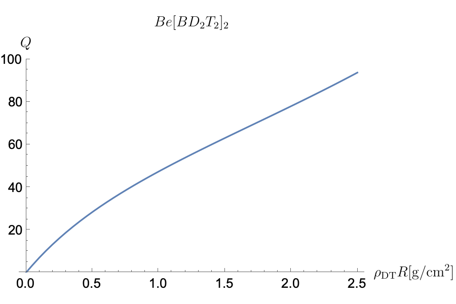
Figure 6: The gain $Q$ as function of $\rho_{\ce{DT}}R$ using (4), (4) and linear interpolation for the ignition temperature $kT_{e}$ obtained from Fig. 2

Next, we consider the case of the fuel $\ce{Be[BD_{2}T_{2}]_{2}}$ with $R=0.02\,\ce{cm}$, $\langle\rho_{\ce{DT}}\rangle R=0.5\,\ce{g}\,\ce{cm^{-2}}$, and $kT_{\ce{e}}=kT_{\ce{i}}=15\,\ce{keV}$ given by the right plots in Fig. 4, which corresponds to a moderate compression by a factor of $\kappa\approx 81$. With these parameters the fuel ignites according to Figs. 2 and 4. The total initial energy for this case is $E\approx 2.98\,\ce{MJ}$. The total fuel mass consisting of $\ce{DT}$ and $\ce{Z}$ is $M\approx 2.1\,\ce{mg}$ suggesting the upper limit $E_{\ce{DT}}\approx 282\,\ce{MJ}$ for the fusion energy assuming $\epsilon_{DT}\approx 17.6\,\ce{MeV}$. The fusion gain predicted by the simulations is $Q\approx 25$, which is in good agreement with Fig. 6. According to Fig. 6 the fusion gain approaches $Q\approx 100$ for $\langle\rho_{\ce{DT}}\rangle R\approx 2.5\,\ce{gcm^{-2}}$.

It is easy to see that the initial ignition temperature depends on the product $E\,\rho^{2}$ for a given $\left\langle\rho_{\ce{DT}}\right\rangle R$. We derive a simple expression for the case of $\ce{Be[BD_{2}T_{2}]_{2}}$. There are

$$N = \frac{\frac{4\pi}{3}R^{3}\rho}{51m_{p}}$$ (5)

fuel molecules, each of which provides $11$ ions and $22$ electrons. This implies under the assumption that $kT_{\ce{e}}=kT_{\ce{i}}$ holds at ignition

$$kT_{e} \approx \frac{102\,m_{p}}{132\,\pi}\frac{E\,\rho^{2}}{\left(\rho R\right)^{3}}\,,$$ (6)

where $\rho=\kappa\,\rho_{\ce{0}}$. For $\rho_{\ce{0}}\approx 0.79\,\ce{gcm^{-3}}$, $\kappa\approx 81$, $R\approx 0.02\,\ce{cm}$ corresponding to $\left\langle\rho_{\ce{DT}}\right\rangle R\approx 0.5\,\ce{gcm^{-2}}$, and $E\approx 2.98\,\ce{MJ}$ the ignition temperature is $kT_{\ce{e}}\approx 15\,\ce{keV}$ in agreement with the iginition temperature in right simulation in Fig. 4. As (6) shows increasing the fuel density implies lower ignition energy. For $\kappa\approx 324$ we obtain $E\approx 186\,\ce{kJ}$.

5 Summary

In the present paper it has been explored under which conditions non-cryogenic DTs are capable of igniting and how their fusion gain scales for volume ignition. As is shown they can yield sufficient fusion gain for fusion energy production. One advantage of non-cryogenic DTs is that they do not require cryo-technology. However, this feature is only one interesting aspect about them. They may also enable potentially simple new fusion reactor designs.

Compared to previous work on non-cryogenic DT fuels [1, 8, 9, 10], we have identified two new important positive effects that improve the predictions for ignition of these fuels and their usage for energy production: 1. Higher ionic than electronic temperatures sustained by 2. significant ionic stopping power in the same order of magnitude as or even exceeding the electronic one. Moreover, with heavy beryllium borohydride we have identified a non-cryogenic DT fuel that ignites more easily than the previously best candidate, heavy beryllium hydride (BeDT).

Volume ignition represents a worst case scenario. Non cryogenic DTs ignite robustly. According to Fig. 6 the fusion gain approaches $Q\approx 100$ for larger $\langle\rho_{\ce{DT}}\rangle R$. The investigation of specific $Q>100$ scenarios with non-cryogenic DTs is left for future work.

6 Acknowledgements

The present work has been funded by Marvel Fusion. Specifically, motivated by the analysis in the present paper Rafael Ramis Abril has adapted the stopping power model for $\alpha$-particles in the original MULTI-IFE code. In addition, neutronic stopping has been added to the code. However, the updated MULTI-IFE code has not been used in the present paper. The consideration of a wider class of fuels beyond DT for fusion energy production has been suggested by Hartmut Ruhl and Georg Korn. The technical details have been worked out by Christian Bild, Matthias Lienert, Markus Nöth, and Hartmut Ruhl. Ondrej Pego Jaura has carried out the simulations. Rafael Ramis Abril has been supported by projects: PID2022-137339OB-C22 of the “Plan Estatal 2021-2023” of the Spanish Goverment and by ENR-IFE.01.CEA of EUROFUSION.

Appendix A Analytical Model

Here we describe the details of our analytical model (1), (2). In A.1, we give the formulas for the loss and gain terms included in the model. Mainly, the deposition power term needs further work. In A.2, we introduce our stopping power model, based on a calculation of friction and heat exchange terms in the Euler equations. In A.3, we consider losses of alpha particles through the boundaries. A.4 deals with neutron scattering. In A.5, we determine the quasi-equilibrium of temperatures that has been used for the plots in sec. 2. In A.6, we calculate the distribution of flight distances inside a sphere for random initial positions and flight directions. A.7 reduces the reactivity for two ion species with different temperatures to the reactivity for a single effective temperature.

A.1 Gains and losses

Here we specify the different gain and loss mechanisms that are taken into account in our analytical model (1), (2).

The most important loss channel is radiation due to bremsstrahlung, given by [15, Eq. 4.24.4]

$$Q_{\mathrm{rad}} = -\frac{2^{1/2}e^{6}}{3\,\pi^{5/2}\epsilon_{0}^{3}c^{3}h\,m_{e}^{3/2}}\,n_{e}\sum_{i}Z_{i}^{2}n_{i}\sqrt{kT_{e}}$$ (7)

with $h$, $e$, $\epsilon_{\ce{0}}$, $c$, and $m_{\ce{e}}$ being Planck’s constant, the elementary charge, the vacuum permittivity, the speed of light and the electron mass, respectively.

Next, we consider heat conduction losses. We take them into account using the formula [11, Eq. 4.10]

$$Q_{\ce{e}} =-\frac{S\chi_{\ce{e}}\nabla kT_{\ce{e}}}{V}\approx-0.5\frac{3\chi_{\ce{e}}kT_{\ce{e}}}{R^{2}}\,,$$ (8)

$$\chi_{e} =\frac{2^{8}\epsilon_{0}^{2}(kT_{e})^{5/2}\sqrt{2\pi}}{\sqrt{m_{e}}q_{e}^{4}\sum_{j}n_{j}}\sum_{i}\frac{n_{i}}{(3.3+Z_{i})\ln\Lambda_{ei}}\,,$$ (9)

where we have chosen the value $0.5$ for the constant $c_{\ce{e}}$ of [11] in accordance with [16, section 2.4]. For the Coulomb logarithm $\ln\Lambda$ we use [17, p. 34] . Our numerical analysis also takes the free streaming limit into account. It is given by

$$Q_{\ce{e}}=-0.1\,\frac{S}{V}n_{e}kT_{e}\sqrt{\frac{kT_{e}}{m_{e}}}\,.$$ (10)

However, this limit only becomes relevant at very high temperatures. Both bremsstrahlung and heat conduction losses affect only the electron temperature.

The heat transfer according to [18] is given by

$$Q_{bc}=\frac{q_{b}^{2}q_{c}^{2}n_{b}n_{c}\ln\Lambda_{bc}}{(2\pi)^{3/2}\epsilon_{0}^{2}m_{b}m_{c}}\frac{kT_{c}-kT_{b}}{\left(\frac{kT_{b}}{m_{b}}+\frac{kT_{c}}{m_{c}}\right)^{3/2}}\,.$$ (11)

Concerning the gain term, we write the overall rate of energy transferred from fusion events to species $b$ as

$$Q_{\mathrm{fus}\rightarrow b} =n_{D}n_{T}\langle\sigma v_{DT}\rangle\left(\langle E^{R}_{\alpha\rightarrow b}\rangle+\langle E^{R}_{n\rightarrow b}\rangle\right)\,,$$ (12)

where $\langle E^{R}_{\alpha\rightarrow b}\rangle$ and $\langle E^{R}_{n\rightarrow b}\rangle$ is the expected energy deposited into species $b$ by an alpha particle and neutron, respectively. The former will be determined in A.3 taking into account stopping power and alpha particles leaving the system due to geometric constraints (see Eq. (34)). The expected deposited energy by neutrons is calculated analogously. In A.4 it is explained how to modify the expression obtained for alpha particles appropriately. For the reactivity $\sigma v_{DT}$, we use the interpolation formula in [19] with the temperature chosen according to (68).

A.2 $\alpha$-stopping

Here we present a method to determine how the energy of the fusion alpha particles is distributed to the different species of charged particles. We assume a homogeneous spherical plasma of electrons, deuterium, tritium, and possibly other ions.

Each alpha particle is created with kinetic energy $E_{\alpha}=3.5\,\mathrm{MeV}$ in the center of mass frame of a pair of deuterium and tritium ions with a uniformly random direction. The velocities of the center of mass frames are distributed thermally with a temperature between the temperatures of the two hydrogen species. The alpha particle energy $3.5\,\mathrm{MeV}$ is overwhelmingly larger than the thermal energies of deuterium and tritium. Hence, the resulting distribution in velocity space at the time of alpha creation is a thin spherical shell with radius $\sqrt{2E_{\alpha}/m_{\alpha}}$ and shell thickness corresponding to the spread in center of mass frames of pairs of deuterium and tritium ions. The precise hydrodynamics of the system containing alpha particles generated according to this distribution, their interaction with the electrons and other ions in the plasma and their influence on the subsequent generation of alpha particles is complicated and only tractable via simulations. In order to generate a semi-analytic model which can be evaluated quickly, we exploit that the density of alpha particles in the plasma is very low until a significant part of the plasma has reacted. Moreover, the density of alpha particles in the $\mathrm{MeV}$-range is low at all times. We follow the alpha particles which are generated at an arbitrary instant. This allows us to dissect the initial velocity space distribution of the alpha particles into many small spherical sectors, each with a mean velocity close to the radius of the sphere and velocity spread close to a thermal distribution with temperature close to the one of the hydrogen species. We take the action of the non-alpha species on the alpha particles into account but neglect any change of properties of the non-alpha species due to the small densities of alpha particles. We also neglect interactions between groups of alpha particles for the same reason.

To derive a one dimensional gain and loss model, we start from the Fokker-Planck equations. Nuclear collision with ions are neglected, even so they increase the ionic stopping power [20]. Its collision operator are given by

$$C(f_{b},f_{c}) = \frac{q_{b}^{2}q_{c}^{2}\ln\Lambda}{8\pi\epsilon_{0}^{2}}\int d^{3}p_{c}\,\left(\frac{\partial}{\partial p^{k}_{b}}-\frac{\partial}{\partial p^{k}_{c}}\right)$$

$$\times\,\frac{|\mathbf{v}|^{2}_{\text{rel}}\delta^{k}_{m}-v^{k}_{\text{rel}}v^{m}_{\text{rel}}}{|\mathbf{v}_{\text{rel}}|^{3}}\left(\frac{\partial}{\partial p^{m}_{b}}-\frac{\partial}{\partial p^{m}_{\ell}}\right)\,f_{b}f_{c}\,.$$

We use an approximation of the eight-moment model of [21, Section 26], [22, Section H], and [23, Equation (73)]. This means we employ the following ansatz for the distribution function to plug into (A.2)

$$f_{b} = \frac{n_{b}}{\left(2\pi m_{b}kT_{b}\right)^{3/2}}\exp\left(-\frac{(\mathbf{p}_{b}-m_{b}\mathbf{u}_{b})^{2}}{2m_{b}kT_{b}}\right)$$

$$\times\,\left[1-\frac{m_{b}}{n_{b}(kT_{b})^{2}}\,\bigg{(}1-\frac{(\mathbf{p}_{b}-m_{b}\mathbf{u}_{b})^{2}}{5m_{b}T_{b}}\bigg{)}\right.$$

$$\hskip 28.45274pt\left.\times\,\mathbf{q}_{b}\cdot\left(\frac{\mathbf{p}_{b}}{m_{b}}-\mathbf{u}_{b}\right)\right]\,.$$

The heat flux $\mathbf{q}_{b}$ is then taken to be zero for the analytical model, because we assume a homogeneous density and temperature. The numerical study treats inhomogeneous fluids by solving the corresponding dynamical equation for the heat flux which follows from (A.2) by a quasi static ansatz. This implies the following Euler equations for multiple species with general mean velocities

$$\frac{dn_{b}}{dt} = -n_{b}\,\frac{\partial}{\partial\mathbf{r}}\cdot\mathbf{u}_{b}\,,$$ (15)

$$m_{b}n_{b}\,\frac{d{\bf u}_{b}}{dt} = -\frac{\partial P_{b}}{\partial\mathbf{r}}+\sum_{\ell}\mathbf{R}_{b\ell}\,,$$ (16)

$$\frac{3}{2}\,n_{b}\,\frac{dkT_{b}}{dt} = -P_{b}\,\frac{\partial}{\partial\mathbf{r}}\cdot\mathbf{u}_{b}-\frac{\partial}{\partial\mathbf{r}}\cdot\mathbf{q}_{b}+\sum_{\ell}Q_{b\ell}\,.$$ (17)

The vector $\mathbf{R}_{b\ell}$ describes the friction between two species, and $Q_{b\ell}$ the heat exchange. The pressure $P_{b}=n_{n}kT_{b}$ satisfies the ideal gas law. Neglecting the heat flux $\mathbf{q}_{b}$, the friction $\mathbf{R}_{b\ell}$ and heat exchange $Q_{b\ell}$ are given by

$$\mathbf{R}_{bc} = \int d^{3}p_{b}\,\mathbf{p}_{b}\,C(f_{b},f_{c})$$

$$= -\frac{q_{b}^{2}q_{c}^{2}n_{b}n_{c}\ln\Lambda_{bc}}{(2\pi)^{3/2}\epsilon_{0}^{2}\mu_{bc}}\,\frac{\mathbf{u}_{bc}}{u_{bc}^{3}}$$

$$\times\,\Psi\left(\frac{u_{bc}}{\sqrt{2\left(\frac{kT_{b}}{m_{b}}+\frac{kT_{c}}{m_{c}}\right)}}\right)$$

and

$$Q_{bc} = \int d^{3}p_{b}\,\frac{1}{2m_{b}}(\mathbf{p}_{b}-m_{b}\mathbf{u}_{b})^{2}\,C(f_{b},f_{c})$$

$$= \frac{q_{b}^{2}q_{c}^{2}n_{b}n_{c}\ln\Lambda_{bc}}{m_{b}(2\pi)^{3/2}\epsilon_{0}^{2}u_{bc}}$$

$$\times\,\Phi\left(\frac{u_{bc}}{\sqrt{2\left(\frac{kT_{b}}{m_{b}}+\frac{kT_{c}}{m_{c}}\right)}},\frac{kT_{b}}{\mu_{bc}\left(\frac{kT_{b}}{m_{b}}+\frac{kT_{c}}{m_{c}}\right)}\right)\,.$$

These quantities are obtained as the first and second moments of the Fokker-Planck collision operator (A.2) assuming local thermal equilibrium (A.2), cf. [21]. The relative velocity is denoted by

$$\mathbf{u}_{bc}=\mathbf{u}_{c}-\mathbf{u}_{c}.$$ (20)

The functions $\Psi$ and $\Phi$ in (A.2) and (A.2) are given by

$$\Psi(x) = \sqrt{\frac{\pi}{2}}\mathrm{erf}\left(x\right)-\sqrt{2}x\exp\left(-x^{2}\right)\,,$$ (21)

$$\Phi(x,y) = \sqrt{\frac{\pi}{2}}\mathrm{erf}\left(x\right)-\sqrt{2}yx\exp\left(-x^{2}\right)\,.$$ (22)

The friction force has two interesting limiting cases given by

$$\frac{1}{u_{\alpha}^{2}}\Psi\left(\frac{u_{\alpha}}{\sqrt{\frac{2kT_{b}}{m_{b}}}}\right)\approx\left\{\begin{matrix}\frac{1}{3}\left(\frac{kT_{b}}{m_{b}}\right)^{-3/2}u_{\alpha},&u_{\alpha}\ll\sqrt{\frac{kT_{b}}{m_{b}}}\\ \sqrt{\frac{\pi}{2}}\,u_{\alpha}^{-2},&u_{\alpha}\gg\sqrt{\frac{kT_{b}}{m_{b}}}\,.\end{matrix}\right.$$ (23)

For low temperatures, the friction with electrons is dominant because of the reduced mass in the denominator of (A.2). Since for electrons the first case of (23) is relevant, their contribution to stopping is reduced when the temperature increases. This increased electron transparency for alpha particles at higher temperatures is a well-known result. For ions on the other hand, the second case of (23) is relevant where the friction is independent of temperature. It is worth noting that the friction term (A.2) is proportional to $Z^{2}$. Hence, at higher temperatures or if medium or high-$Z$ materials are present, the ion contribution to alpha stopping starts to play an important role.

Energy conservation is given by

$$Q_{bc}+Q_{cb}=\mathbf{R}_{bc}\cdot\mathbf{u}_{bc}\,.$$ (24)

Accordingly, $Q_{bc}$ describes two effects. First, it describes how the heat that is generated by friction is distributed between both species. Second, if the two temperatures differ, then heat flows between those species. In the limit of $u_{b\ell}\rightarrow 0$ the term $Q_{bc}$ reduces to (11). It is the goal of this section to determine the frictional heat deposition in alpha particles and the other species and the subsequent temperature flow from the alpha particles to the other species. To this end, we solve the hydrodynamic equations in Lagrangian coordinates, neglecting the pressure terms, as friction has a much greater effect for such high relative velocities:

$$\frac{du_{\alpha}}{dt}=\sum_{\ell}\frac{R_{\alpha\ell}}{m_{\alpha}n_{\alpha}}\,,$$ (25)

$$\frac{d(kT_{\alpha})}{dt}=\sum_{\ell}\frac{2Q_{\alpha\ell}}{3n_{\alpha}}\,.$$ (26)

Since all non alpha species are on average at rest, $u_{\alpha\ell}=u_{\alpha}=\sqrt{\frac{2E_{\alpha}}{m_{\alpha}}}$. We parameterize the dynamics with respect to flight distance instead of the time and we use the energy instead of the velocity, arriving at

$$\frac{dE_{\alpha}}{dx} = \sum_{\ell}\frac{-m_{\alpha}q_{\alpha}^{2}q_{\ell}^{2}n_{\ell}\ln\Lambda_{\alpha\ell}}{2(2\pi)^{3/2}\epsilon_{0}^{2}\mu_{\alpha\ell}E_{\alpha}}$$

$$\times\,\Psi\left(\sqrt{\frac{E_{\alpha}}{m_{\alpha}\left(\frac{kT_{\alpha}}{m_{\alpha}}+\frac{kT_{\ell}}{m_{\ell}}\right)}}\right)$$

$$\frac{dkT_{\alpha}}{dx} = \sum_{\ell}\frac{q_{\alpha}^{2}q_{\ell}^{2}n_{\ell}\ln\Lambda_{\alpha\ell}}{3(2\pi)^{3/2}\epsilon_{0}^{2}E_{\alpha}}$$

$$\times\,\Phi\left(\sqrt{\frac{E_{\alpha}}{m_{\alpha}\left(\frac{kT_{\alpha}}{m_{\alpha}}+\frac{kT_{\ell}}{m_{\ell}}\right)}},\frac{kT_{\alpha}}{\mu_{\alpha\ell}\left(\frac{kT_{\alpha}}{m_{\alpha}}+\frac{kT_{\ell}}{m_{\ell}}\right)}\right)$$

These are two coupled differential equations, which depends on the constants $kT_{\ell}$. We integrate them up to a distance $\min(s,s_{\alpha})$. Here, $s$ is the distance the alpha particles travel until they leave the fuel and $s_{\alpha}$ is the distance until they lose $99\%$ of the sum of their kinetic energy and the difference of their initial and final thermal energies.

The criterion to determine the exact value of $s_{\alpha}$ has a weak influence on the energy distribution. When the alpha particles are almost at rest, their kinetic energy decreases exponentially. Hence, the stopping process is at no point in time concluded. During this process, the alphas continuously act as thermal bridge between the other species. Thus, some choice when to stop the dynamics has to be made. We use the $99\%$ criterion which has the additional advantage of avoiding numerical instabilities at the end of the dynamics. The amount of heat transferred to the non alpha species $E_{b}=\frac{3}{2}n_{b}kT_{b}$ per alpha particle can be obtained from the following equations.

$$\frac{dE_{b}}{dx} = \frac{m_{\alpha}q_{b}^{2}q_{\alpha}^{2}n_{b}\ln\Lambda_{b\alpha}}{m_{b}2(2\pi)^{3/2}\epsilon_{0}^{2}E_{\alpha}}$$

$$\times\,\Phi\left(\sqrt{\frac{E_{\alpha}}{m_{\alpha}\left(\frac{kT_{b}}{m_{b}}+\frac{kT_{\alpha}}{m_{\alpha}}\right)}},\frac{kT_{b}}{\mu_{b\alpha}\left(\frac{kT_{b}}{m_{b}}+\frac{kT_{\alpha}}{m_{\alpha}}\right)}\right),$$

$$E^{s}_{\alpha\rightarrow b} = \int_{0}^{\min(s,s_{\alpha})}dx\,\frac{dE_{b}}{dx}\,.$$ (30)

We solve these equations numerically for a given state of the fuel and a distance $s$ for the analysis in the main text.

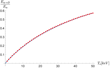
Figure 7: Energy transfer to deuterium ions via $\alpha$-stopping in a deuterium electron plasma for $kT_{\ce{e}}=kT_{\ce{D}}$ calculated with the model in this paper (red dots) and the model in  [15, Eq. 5.4.12] (blue line).

In order to compare our model with the literature, we note that [15, chapter 5.4] contains a similar model but only for the special case of equal ion and electron temperatures. The energy transfer to ions for the two models is compared in Fig. 7 for a deuterium electron plasma with equal temperatures, showing excellent agreement.

The next section discusses the losses of due to alpha particles leaving the plasma.

A.3 $\alpha$-losses

We now assess the alpha losses associated with finite size, considering a homogeneous spherical plasma with radius $R$.

Some alpha particles will leave the plasma before they are fully stopped. To estimate the associated energy loss, we assume that the generation of alpha particles is equally likely everywhere inside the sphere and that every flight direction is equally likely. In order to calculate the energy deposition, it is sufficient to know the distribution $p(s)$ of the lengths of the trajectories $s$ inside the plasma. It will be determined in A.6, with the result (62). For any length $s$, the deposited energy is given by Eq.(30). Then the mean deposited energy is given by the average of that expression, i.e., by

$$\langle E^{R}_{\alpha\rightarrow b}\rangle=\int_{0}^{2R}ds\,p(s)\int_{0}^{\min(s,s_{\alpha})}\frac{dE_{b}(E_{\alpha}(x))}{dx}dx.$$ (31)

Using partial integration, we simplify this expression to

$$\langle E^{R}_{\alpha\rightarrow b}\rangle =\int_{0}^{\min(2R,s_{\alpha})}\frac{dE_{b}(E_{\alpha}(x))}{dx}dx$$

$$-\int_{0}^{\min(2R,s_{\alpha})}\frac{s(12R^{2}-s^{2})}{16R^{3}}\frac{dE_{b}(E_{\alpha}(s))}{dx}ds$$ (32)

$$=E^{\infty}_{\alpha\rightarrow b}-\mathds{1}_{2R<s_{\alpha}}\int_{2R}^{s_{\alpha}}\frac{dE_{b}(E_{\alpha}(x))}{dx}dx$$

$$-\int_{0}^{\min(2R,s_{\alpha})}\frac{s(12R^{2}-s^{2})}{16R^{3}}\frac{dE_{b}(E_{\alpha}(s))}{ds}ds$$ (33)

$$=E^{\infty}_{\alpha\rightarrow b}-\langle L^{R}_{\alpha\rightarrow b}\rangle$$ (34)

where $E^{\infty}_{\alpha\rightarrow b}$ is given by (30) corresponding to an infinitely extended plasma with no alpha losses.

The first of the two loss terms corresponds to the energy that an alpha particle would transfer to the species $b$ if it could stay inside the plasma even after traversing a distance of $2R$. This term only contributes for $2R<s_{\alpha}$. The second term never vanishes as it includes losses due to outward-moving alpha particles that are created close to the boundary of the plasma. The overall rate of energy transferred from alpha particles created in fusion events to species $b$ (12) can be split into a gain and a loss term:

$$Q_{\mathrm{fus}\rightarrow b}^{\alpha}=n_{D}n_{T}\langle\sigma v_{DT}\rangle(E^{\infty}_{\alpha\rightarrow b}-\langle L^{R}_{\alpha\rightarrow b}\rangle)$$ (35)

$$=Q^{\infty}_{\mathrm{fus}\rightarrow b}-Q_{b\rightarrow\mathrm{loss}}.$$ (36)

The total fusion power thus also splits into a gain and a loss term

$$\sum_{\ell}Q^{\infty}_{\mathrm{fus}\rightarrow\ell}-\sum_{\ell}Q_{\ell\rightarrow\mathrm{loss}}=Q_{\mathrm{fus}}-Q_{\mathrm{fus}\rightarrow\mathrm{loss}}.$$ (37)

A.4 Neutron scattering

The neutron energy deposition is calculated with an analogous model as the alpha energy deposition. The only difference is that the formulas for $\mathbf{R}_{b\ell}$ and $Q_{b\ell}$ in (16) and (17) need to be changed. For the neutron ion interaction we model the collisions as hard sphere collisions, as is implicitly assumed in [11] and [1]. This model slightly overestimates the neutron stopping since the the differential cross sections for elastic collisions with ions are not constant, as they would be for hard spheres, but smaller for high scattering angles. Large scattering angles, however, result in high energy transfer to the collision partners and a larger reduction of the mean velocity. This is partially compensated by the fact that we neglect inelastic scattering and also that we assume energy independent cross sections and choose the value at $14\mathrm{MeV}$, although the cross section is considerably higher for smaller energies. For hard spheres, the friction functions $R,Q$ haven been worked out in [21, Eq. 15.14 and 15.15]

$$\mathbf{R}_{bc} =-n_{b}m_{b}\nu_{bc}u_{bc}\Psi\left(\epsilon_{bc}\right)\,,$$ (38)

$$Q_{bc} =\frac{m_{b}}{m_{b}+m_{c}}\,n_{b}\nu_{bc}$$ (39)

$$\hskip 11.38092pt\times\left[3\left(kT_{c}-kT_{b}\right)\,\Phi\left(\epsilon_{bc}\right)+m_{c}u^{2}_{bc}\,\Psi\left(\epsilon_{bc}\right)\right]\,,$$

where

$$\nu_{bc} =\frac{8}{3\sqrt{\pi}}\frac{n_{c}m_{c}}{m_{b}+m_{c}}\sqrt{2\left(\frac{kT_{b}}{m_{b}}+\frac{kT_{c}}{m_{c}}\right)}\,\sigma_{bc}$$ (40)

and

$$\Psi\left(\epsilon_{bc}\right) =\frac{3\sqrt{\pi}}{8}\,\left(\epsilon_{bc}+\frac{1}{\epsilon_{bc}}-\frac{1}{4\epsilon^{3}_{bc}}\right)\,\mathrm{erf}\left(\epsilon_{bc}\right)$$ (41)

$$\hskip 28.45274pt+\frac{3}{8}\left(1+\frac{1}{2\epsilon^{2}_{bc}}\right)e^{-\epsilon^{2}_{bc}}\,,$$

$$\Phi\left(\epsilon_{bc}\right) =\frac{\sqrt{\pi}}{2}\left(\epsilon_{bc}+\frac{1}{2\epsilon_{bc}}\right)\mathrm{erf}\left(\epsilon_{bc}\right)+\frac{1}{2}e^{-\epsilon^{2}_{bc}}\,,$$ (42)

with

$$\epsilon_{bc} =\frac{|u_{bc}|}{\sqrt{2\left(\frac{kT_{b}}{m_{b}}+\frac{kT_{c}}{m_{c}}\right)}}\,.$$ (43)

Here, $u_{bc}=u_{n}$ since the ion species are considered to have no mean velocity in our model. Making use of (16) and (38) - (43) we obtain a coupled system of ODEs for the kinetic energy of a group of neutrons with small angular spread in velocities and temperature analogous to the one for $\alpha$-stopping:

$$\frac{dE_{n}}{dx} =-\sqrt{2m_{n}E_{n}}\,\sum_{c}\nu_{nc}\,\Psi\left(\epsilon_{nc}\right)\,,$$ (44)

$$\frac{d\,kT_{n}}{dx} =\frac{2}{3}\,\sqrt{\frac{m_{n}}{2E_{n}}}\,\sum_{c}\frac{m_{n}}{m_{n}+m_{c}}\,\nu_{nc}$$ (45)

$$\hskip 11.38092pt\times\left[3\left(kT_{c}-kT_{n}\right)\Phi\left(\epsilon_{nc}\right)+\frac{2\,m_{c}}{m_{n}}\,E_{n}\,\Psi\left(\epsilon_{nc}\right)\right]\,,$$

where

$$\epsilon_{nc} =\sqrt{\frac{m_{c}\,E_{n}}{m_{n}\,kT_{c}+m_{c}\,kT_{n}}}\,.$$ (46)

It is also possible to obtain the energy a typical neutron transfers to the ion fluid $b$. We define

$$\zeta_{b} =\frac{3}{2}\,\frac{n_{b}}{n_{n}}\,kT_{b}\,.$$ (47)

Replacing the index $n$ by $b$ and the index $c$ by $n$ in (45) and making use of (47) we obtain

$$\frac{d\zeta_{b}}{dx} =\sqrt{\frac{m_{n}}{2E_{n}}}\,\frac{m_{b}}{m_{n}+m_{b}}\,\frac{n_{b}}{n_{n}}\,\nu_{bn}$$ (48)

$$\hskip 11.38092pt\times\left[3\left(kT_{n}-kT_{b}\right)\,\Phi\left(\epsilon_{nb}\right)+2E_{n}\,\Psi\left(\epsilon_{nb}\right)\right]\,.$$

Equations (48) have to be solved in line with (44) and (45). The solution of these equations determines the heat transport per neutron to species $b$. The average neutron energy deposition into species $b$ is obtained by substituting $\frac{d\zeta_{b}}{dx}$, given by (48), for $\frac{dE_{b}}{dx}$ in (34). The result is $\langle E^{R}_{n\rightarrow b}\rangle$.

In the following, we approximate the above expressions for large velocities $u_{n}$ in order to compare our model with elementary considerations. We obtain:

$$\Psi\left(\epsilon_{nc}\right) =\frac{3\sqrt{\pi}}{8}\,\epsilon_{nc}\,,\quad\Phi\left(\epsilon_{nc}\right)=\frac{\sqrt{\pi}}{2}\epsilon_{nc}\,.$$ (49)

Treating all ions in the fuel as heavier than the neutrons and that all scattering cross sections between neutrons and fuel ions as approximately equal, i.e., $m_{c}\gg m_{n}$, $\sigma_{nc}\approx\sigma_{n}$ and

$$\sum_{c}\nu_{nc}\,\Psi\left(\epsilon_{nc}\right) \approx\left|u_{n}\right|\,\sigma_{n}\,\sum_{c}n_{c}\,.$$ (50)

Making use of (44), (48), and (50) leads to

$$\frac{dE_{n}}{dx} \approx-\sqrt{2m_{n}E_{n}}\,\left|u_{n}\right|\,\sigma_{n}\,\sum_{c}n_{c}$$ (51)

and

$$\frac{dE_{n}}{dt} \approx-2\,\left(\left|u_{n}\right|\,\sigma_{n}\,\sum_{c}n_{c}\right)\,E_{n}\,,$$ (52)

$$\frac{d\zeta_{b}}{dt} \approx+2\,\left(\frac{n_{b}}{n_{n}}\,\left|u_{n}\right|\,\sigma_{n}\,n_{b}\right)\,E_{n}\,.$$ (53)

Equations (52) and (53) can also be inferred from elementary considerations. They imply that neutronic energy deposition in non-cryogenic DT can be considerable and that neutrons heat light fuel ions directly.

A.5 Stationary temperature analysis

Here we determine the quasi-equilibrium mentioned in sec. 2 by keeping the electron temperature fixed and studying the equilibrium temperatures that establish themselves for the ions via Eqs. (1), (2). The validity of this quasi-equilibrium depends on the time scales of equilibration for ions and electrons. The flow diagram 1 shows that the ions do, indeed, reach their equilibrium faster than the electrons. Note that in any case, the fixed points lie on the line of quasi-equilibrium, as at those points the electron temperature is constant. One can thus regard this notion of quasi-equilibrium as a simplified tool in the analysis of the temperature flow diagram 1.

The only relevant gain and loss mechanisms for ions are the stopping of fusion alpha particles and neutrons (12) as well as heat transfer to other particle species (11). Now, quasi-equilibrium is reached when gains and losses exactly compensate each other. Hence, we have for all ion species $i$:

$$\sum_{\ell}Q_{i\ell}+Q_{\mathrm{fus}\rightarrow i}=0\,.$$ (54)

For $n$ different species, one of them electrons with a given temperature $kT_{e}$, (54) is a system of $n-1$ equations for $n-1$ ion temperatures $kT_{i}$. This system of equations can be solved numerically, yielding $n-1$ functions $kT_{i}(kT_{e})$.

In equilibrium, the ions receive energy from alpha particles and can only pass on this energy to electrons. However, this is only possible for $kT_{i}>kT_{e}$. How much higher the different $kT_{i}$ are than $kT_{e}$ strongly depends on alpha and neutron stopping of the ion species. This effect therefore varies with fuel composition and electron temperature. The resulting difference in ion and electron temperatures is a useful effect for fusion applications since it leads to an increased fusion rate compared to radiation losses.

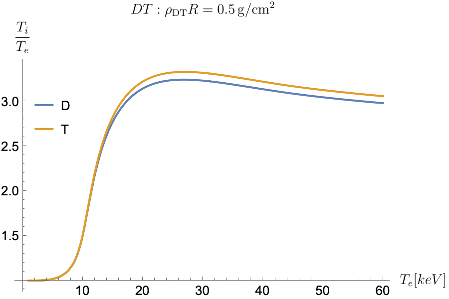
Figure 8: Ratio of ion temperatures to electron temperature given by the solution of (54) for a range of electron temperatures for DT showing that $kT_{\ce{D}},kT_{\ce{T}}\gg kT_{\ce{e}}$ for $kT_{\ce{e}}>10\,\ce{keV}$.

We illustrate the dependence of $kT_{i}$, $i=D,T$ on $kT_{e}$ in Fig. 8 for DT. At temperatures below $10\,\mathrm{keV}$, we see $kT_{i}\approx kT_{e}$. Above this threshold, the ionic temperatures rise up to $kT_{i}\approx 3kT_{e}$. The detailed balance of energy flux at $kT_{e}=30\,\mathrm{keV}$ is shown in Fig. 9.

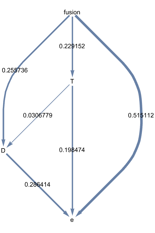
Figure 9: Fraction of fusion power transferred between the different species for an equal mixture of $D$ and $T$ at $\rho_{\mathrm{DT}}R=0.5g\mathrm{cm}^{-2}$. The ion temperatures in conditional equilibrium for $kT_{e}=30\,keV$ are $kT_{D}=97.1\,keV$ and $kT_{T}=99.7\,keV$.

A.6 Distribution of distances

Here we derive the distribution of geometric flight distances of alpha particles inside a homogeneous ball of radius $R$ similar to [24]. Hence, the stopping of alpha particles will play no role in this derivation. We assume that the alpha particles are equally likely to be created at any point inside the ball, parameterised by the coordinates $r,\theta_{1}$ and $\varphi_{1}$, and equally likely to have their initial velocity point in any direction, parameterised by the coordinates $\theta_{2}$ and $\varphi_{2}$. The angle $\theta_{2}$ for the flight direction is chosen relative to the line connecting the initial position of the particle and the center of the sphere. The distance $s$ follows from the law of cosines

$$r^{2}+s^{2}-2rs\cos(\theta_{2})=R^{2}\,.$$ (55)

We can write the cumulative distribution function of the distances as

$$P(s\leq S) =\frac{3}{(4\pi)^{2}R^{3}}\int_{0}^{2\pi}d\varphi_{1}\int_{0}^{\pi}d\theta_{1}\sin\theta_{1}\int_{0}^{R}dr\,r^{2}$$ (56)

$$~{}~{}\int_{0}^{\pi}d\theta_{2}\sin\theta_{2}\int_{0}^{2\pi}d\varphi_{2}\mathds{1}_{s(r,\theta_{2})\leq S}$$ (57)

$$=\frac{3}{2R^{3}}\int_{0}^{R}dr\int_{-1}^{1}dw~{}r^{2}\mathds{1}_{s(r,w)\leq S}.$$ (58)

The boundary between the regions $s(r,w)\leq S$ and $s(r,w)>S$ in the $r,w$ coordinate space is given by

$$w=\frac{r^{2}+S^{2}-R^{2}}{2rS}\,.$$ (59)

For any given value of $S$, the point $(r,w)=(R,1)$ in the upper right corner of the integration domain corresponds to the maximal value $s(r,w)=2R$. Therefore, it is inside the region $s(r,w)>S$ that is not contributing to the integration for all values $S<2R$. Therefore $w$ should be integrated over all values less than the one singled out by Eq. (59). The boundary Eq. (59) intersects the boundaries of the integration domain at $r=S-R,w=1$ for $S>R$ and at $r=R-S,w=-1$ for $S<R$ as exemplified in Fig. 10. This leads to the two cases

$$P(s\leq S)=\frac{3}{2R^{3}}\left\{\begin{matrix}[l]\int_{0}^{S-R}drr^{2}\int^{1}_{-1}dw&S>R\\ \hskip 14.22636pt+\int^{R}_{S-R}drr^{2}\int_{-1}^{\frac{r^{2}+S^{2}-R^{2}}{2rS}}dw&\\ \int_{R-S}^{R}drr^{2}\int_{-1}^{\frac{r^{2}+S^{2}-R^{2}}{2rS}}dw&S<R\end{matrix}\right.$$ (60)

Both cases lead to the same value

$$P(s\leq S)=\frac{S(12R^{2}-S^{2})}{16R^{3}}$$ (61)

resulting in the probability density

$$p(S)=\frac{\partial}{\partial S}P(s\leq S)=\frac{3}{4R}-\frac{3}{16}\frac{S^{2}}{R^{3}}\,,$$ (62)

which is shown in Fig. 11.

Figure 10: The integration boundary (59) for two different values of $S$. For $S=1.4R$ the area of integration $s\leq 1.4R\wedge|w|<1\wedge 0<r<R$ is bounded from above by $w=1$ for $r<0.4R$ and by (59) for $r>0.4R$. For $S=0.9R$ the integration region $s\leq 0.9R\wedge|w|<1\wedge 0<r<R$ begins at $r=0.1R$ and is bounded from above by (59).

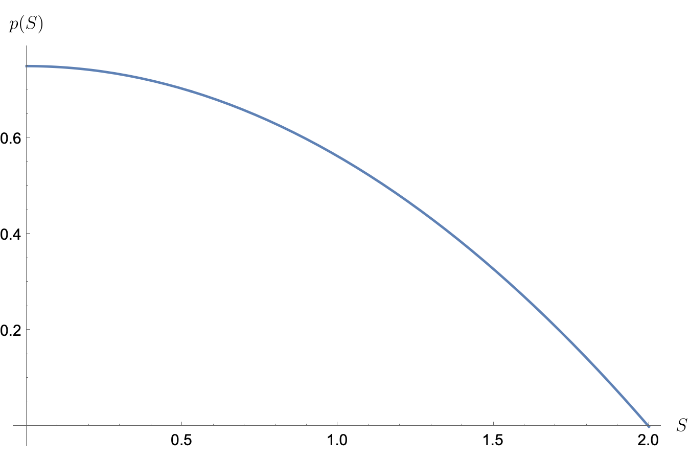
Figure 11: The probability distribution for the expected geometric flight distance $S$ of the alphas (62) for $R=1$. Without stopping power of the plasma, the alphas would on average cover a distance of $\frac{3}{4}R$ before leaving the fuel.

A.7 Reactivity for mixed temperatures

In this section, we describe how to obtain the reactivity for a fusion reaction between two different ion species, $i$ and $\ell$, which have different temperatures $kT_{i}$ and $kT_{\ell}$. This is necessary as we allow for different temperatures of the different ionic species.

One needs to calculate

$$\langle\sigma(v_{rel})v_{rel}\rangle=\int f_{i}f_{\ell}\sigma(v_{rel})v_{rel}d^{3}v_{i}d^{3}v_{\ell}$$ (63)

where

$$f_{b}=\frac{n_{b}}{\left(2\pi kT_{b}/m_{b}\right)^{3/2}}\exp\left(-\frac{m_{b}v_{b}^{2}}{2kT_{b}}\right)$$ (64)

for $b=i,\ell$. To simplify (63), the center of mass and relative velocity coordinates need to be modified and temperature weighted, leading to

$$\mathbf{U} =\frac{\frac{m_{i}}{kT_{i}}\mathbf{v}_{i}+\frac{m_{\ell}}{kT_{\ell}}\mathbf{v}_{\ell}}{\frac{m_{i}}{kT_{i}}+\frac{m_{\ell}}{kT_{\ell}}},$$ (65)

$$\mathbf{v}_{rel} =\mathbf{v}_{i}-\mathbf{v}_{\ell},$$ (66)

$$f_{i}f_{\ell} =\frac{n_{i}n_{\ell}}{\left(4\pi^{2}kT_{i}kT_{\ell}/(m_{i}m_{\ell})\right)^{3/2}}$$

$$\times\exp\left(-\left(\frac{m_{i}}{kT_{i}}+\frac{m_{\ell}}{kT_{\ell}}\right)\frac{U^{2}}{2}-\frac{\frac{m_{i}}{kT_{i}}\frac{m_{\ell}}{kT_{\ell}}}{\frac{m_{i}}{kT_{i}}+\frac{m_{\ell}}{kT_{\ell}}}\frac{v_{rel}^{2}}{2}\right)\,.$$ (67)

For equal temperatures, the prefactor of $v_{rel}^{2}$ in (67) is given by $\mu/(2kT)$, where $\mu=m_{i}m_{\ell}/(m_{i}+m_{\ell})$ is the reduced mass. A comparison with (67) shows that the reactivity in the two temperature case can be reduced to that for a single temperature given by

$$kT=\frac{m_{i}kT_{\ell}+m_{\ell}kT_{i}}{m_{i}+m_{\ell}}\,.$$ (68)

A.8 Radiation Losses

Based on a similar ”ray tracing” model as for the alpha particles, we here determine how much of the radiation gets reabsorbed due to the opacity of the fuel. Moreover, we compare the result to another analytical model based on the radiation diffusion equations that MULTI implements for a simplified case.

We are interested in the radiation power for the frequency $\nu$ that escapes the fuel sphere. To this end, we imagine that each photon is generated at a randomly uniform position within the fuel sphere and with a randomly uniform flight direction. Since this is analogous our previous model for alpha particles and neutrons, we can re-use formula (62) for the distribution of flight distances. Then $L_{\nu}$ can be obtained by integrating the emissivity $\eta_{\nu}$ over all initial positions (factor $\frac{4\pi}{3}$), flight directions (factor $4\pi$) and flight distances $s$ weighted with the probability (62) for the flight distance $s$ multiplied by the probability $\exp(-\kappa_{\nu}^{\prime}s)$ that the photon does not get absorbed after a distance $s$. Here, $\kappa^{\prime}_{\nu}=(1-\exp(-h\nu/kT))\kappa_{\nu}$ is the relevant opacity (compare [11, chap. 7.3.2]) which is related to $\eta_{\nu}$ via Kirchhoff’s law $\eta_{\nu}=\kappa^{\prime}_{\nu}I_{P\nu}$ where $I_{P\nu}$ is the Planck intensity. This yields

$$L_{\nu} =\frac{4}{3}\pi R^{3}\eta_{\nu}\,4\pi\int_{0}^{2R}ds\left(\frac{3}{4R}-\frac{3}{16}\frac{s^{2}}{R^{3}}\right)\exp(-\kappa^{\prime}_{\nu}s)$$ (69)

$$=4\pi^{2}R^{2}I_{P\nu}\left(1-\frac{1-\exp(-2\kappa^{\prime}_{\nu}R)(1+2\kappa^{\prime}_{\nu}R)}{2{\kappa^{\prime}}^{2}_{\nu}R^{2}}\right)\,.$$

With the expression for the opacity [11, eqs. 10.91, 10.92] corresponding to (7),

$$\kappa^{\prime}_{\nu} =\left[1-\exp\left(-h\nu/(kT)\right)\right]\,$$ (70)

$$\times\frac{2\sqrt{3}}{\pi}\frac{16\pi}{3\sqrt{6\pi}}\frac{e^{6}}{\left(4\pi\epsilon_{0}\right)^{3}m_{e}^{3/2}c}\frac{n_{e}\sum_{i}Z_{i}^{2}n_{i}}{\sqrt{kT}}\frac{1}{2h\nu^{3}}$$

$$=\underbrace{\frac{16}{3\sqrt{2\pi}}\frac{e^{6}}{\left(4\pi\epsilon_{0}\right)^{3}m_{e}^{3/2}c}\frac{n_{e}\sum_{i}Z_{i}^{2}n_{i}}{(kT)^{7/2}}h^{2}R}_{=:x}\frac{1}{R}\frac{1-\exp(-u)}{u^{3}}$$

$$=\frac{x}{R}\frac{1-\exp(-u)}{u^{3}}$$

it follows that the total radiation loss power estimated by ”ray tracing” is given by

$$L_{\mathrm{ray}}:=\int_{0}^{\infty}d\nu\,L_{\nu}=4\pi^{2}R^{2}\left(\frac{kT}{h}\right)^{4}\frac{2h}{c^{2}}\int_{0}^{\infty}du\,\frac{u^{3}}{\exp(u)-1}$$

$$\times\left(1-\frac{1-\exp\Big{(}-2x\frac{1-\exp(-u)}{u^{3}}\Big{)}\Big{(}1+2x\frac{1-\exp(-u)}{u^{3}}\Big{)}}{2\left(x\frac{1-\exp(-u)}{u^{3}}\right)^{2}}\right)\,.$$ (71)

This integral is approximately equal to $\text{min}(\frac{4}{3}\log(1+x),\frac{\pi^{4}}{15})$, but we use numerical solutions. We estimate

$$\text{for }x\ll\text{1: }L_{\mathrm{ray}} =\frac{4}{3}\pi R^{3}Q_{\mathrm{rad}}\,,$$ (72)

$$\text{for }x\gg\text{1: }L_{\mathrm{ray}} =4\pi R^{2}\sigma T^{4}\,,$$ (73)

where $Q_{rad}$ is given by Eq. (7) and $\sigma$ is the Stefan-Boltzmann constant. Hence, (71) interpolates between optically thin plasma for $x\ll 1$ and optically thick plasma for $x\gg 1$. It can be seen in Fig. 12 that especially at lower temperatures the radiation re-absorption does reduce the radiation losses considerably. However, we emphasize that the results for the analytical model in the main text do not take into account radiation re-absorption as it breaks the simple $\rho_{\ce{DT}}R$ scaling. We hence obtain a conservative estimate.

The MULTI-IFE code, however, uses a different method to estimate the radiation losses. It solves the multi-group radiation equations ($i$ being the radiation group index)

$$\nabla\cdot\mathbf{S}^{i} =c\kappa^{Pi}(U^{Pi}(T)-U^{i})\,,$$ (74)

$$\mathbf{S}^{i} =-\frac{c}{3\kappa^{Ri}}\nabla U^{i}\,.$$ (75)

For the simple scenario of a hot spherical plasma with constant temperature $T$ and constant Rosseland and Planck opacities $\kappa_{h}^{Ri},\kappa_{h}^{Pi}$ surrounded by a cold medium with $T=0$ and also constant opacities $\kappa_{c}^{Ri},\kappa_{c}^{Pi}$, those equations can be solved analytically

$$\Delta U^{i} = \frac{1}{r}\partial_{r}^{2}(rU^{i})=3\kappa^{Ri}\kappa^{Pi}(U^{i}-U^{Pi}(T))$$ (76)

$$U_{h}^{i} = c^{i}_{1}\frac{\exp(\sqrt{3\kappa^{Ri}_{h}\kappa^{Pi}_{h}}r)}{r}$$

$$+c^{i}_{2}\frac{\exp(-\sqrt{3\kappa^{Ri}_{h}\kappa^{Pi}_{h}}r)}{r}+U^{Pi}(T)$$

$$U^{i}_{c} = c^{i}_{3}\frac{\exp(\sqrt{3\kappa^{Ri}_{c}\kappa^{Pi}_{c}}r)}{r}$$

$$+c_{4}^{i}\frac{\exp(-\sqrt{3\kappa^{Ri}_{c}\kappa^{Pi}_{c}}r)}{r}\,.$$

Here, $U^{Pi}(T)=\frac{4\pi}{c}\int_{\nu_{i-1}}^{\nu_{i}}\,I_{P\nu}(T)$. Physical solutions require $c^{i}_{3}=0$ and that $c^{i}_{2}=-c^{i}_{1}$ and continuity of $U^{i}$ and $\mathbf{S}^{i}$ at $r=R$, from which $c^{i}_{1}$ and $c^{i}_{4}$ can be determined. With (75), the total radiation outflow $\mathbf{S}^{i}(R)$ of the hot sphere is determined. Here, the case of a surrounding vacuum is needed. It is obtained by taking the limit $\kappa_{c}^{Ri},\kappa_{c}^{Pi}\rightarrow 0$ for $\mathbf{S}^{i}(R)$, leading to

$$\mathbf{S}^{i}(R) =\left(\sqrt{\frac{\kappa^{Pi}_{h}}{3\kappa^{Ri}_{h}}}\coth(\sqrt{3\kappa^{Ri}_{h}\kappa^{Pi}_{h}}R)-\frac{1}{3\kappa^{Ri}_{h}R}\right)cU^{Pi}(T)\,.$$ (79)

In the limit of infinitely many groups, we have $\kappa^{Ri}_{h}=\kappa^{Pi}_{h}=\kappa^{\prime}_{v}$. Using the analytic expression (70) for $\kappa^{\prime}_{v}$, we obtain

$$L_{\infty} =\int_{0}^{\infty}d\nu\,4\pi R^{2}\,\mathbf{S}^{i}(R)$$ (80)

$$=R^{2}\left(\frac{kT}{h}\right)^{4}\frac{32\pi^{2}h}{c^{2}}\int_{0}^{\infty}du\frac{u^{3}}{\exp(u)-1}$$

$$\times\left(\frac{1}{\sqrt{3}}\coth\left(\sqrt{3}x\frac{1-\exp(-u)}{u^{3}}\right)-\frac{u^{3}}{3x(1-\exp(-u))}\right)\,.$$

While this formula has the same optically thin limit (72), in the case for optically thick plasma (73), there is an additional factor $4/\sqrt{3}$. Since this case is not relevant for the scenarios investigated here, we abstain from further discussing this factor.

For a finite number $G$ of groups the total radiation loss power is given by

$$L_{\mathrm{G}}=\, 4\pi R^{2}\sum_{i}^{\mathrm{G}}\left(\sqrt{\frac{\kappa^{Pi}_{h}}{3\kappa^{Ri}_{h}}}\coth(\sqrt{3\kappa^{Ri}_{h}\kappa^{Pi}_{h}}R)-\frac{1}{3\kappa^{Ri}_{h}R}\right)$$ (81)

$$\times\int_{\nu_{i-1}}^{\nu_{i}}d\nu\frac{8\pi h\nu^{3}}{c^{2}}\frac{1}{\exp(h\nu/kT)-1}\,.$$

To compare more directly with the MULTI code, we evaluate this analytically determined function using the same numerical opacity tables [25](TOPS Opacities). Fig. 12 shows that the different models for the radiation losses are in close agreement.

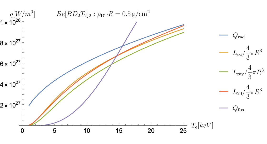
Figure 12: Total radiation power density according to the different models together with the fusion power density for $\ce{Be[BD_{2}T_{2}]_{2}}$, $\rho_{\mathrm{DT}}=50\,\ce{gcm^{-3}}$, and $R=0.01\,\ce{cm}$. The unmitigated radiation loss power $Q_{\ce{rad}}$, which is used in the main text leads to the highest radiation losses. The effect of radiation re-absorption is strongest at low temperatures as the $T^{-3.5}$ dependence of the opacity (70) suggests. The different results $L_{\ce{ray}}$ (71) and the multi group results $L_{20}$ and $L_{\infty}$ (81) agree closely. For the fusion power, the quasi equilibrium temperatures have been used.

Appendix B Modifications to MULTI-IFE

To accommodate active and inactive mass densities $\rho_{\ce{DT}}$ and $\rho_{\ce{Z}}$ within the framework of MULTI-IFE without substantial modifications to the code at this time we introduce alternating layers of active $\ce{DT}$ and inactive $\ce{Z}$ materials (see Fig. 13).

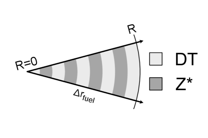
Figure 13: Alternating layers setup. The simulation volume $r<r_{\mathrm{fuel}}$ is filled with alternating layers of reactive (DT) and non-reactive (Z*) materials.

The layering changes the balance of fusion power and radiation losses compared to a homogeneous mixture with a certain value of $\rho_{\ce{DT}}R$. To create a layered scenario which is comparable with the homogeneous mixture, we use DT layers with the density $2\rho_{\ce{DT}}$ and Z* layers with the density $2\rho_{\ce{Z}}$ as well as the radius of the layered construction $R_{\ce{layers}}$ being equal to the unlayered one. Then the average densities are the same in both the layered and unlayered cases.

We consider a layer of thickness $2\Delta R$ of the homogeneous mixture. In the layered construction it gets replaced by a DT layer and a Z* layer, each of thickness $\Delta R$. The fusion power generated by this layered construction is increased by a factor of two compared to the homogeneous mixture in the unlayered construction as the DT density is doubled (and enters fusion power quadratically) but occupies only half the volume [16].

However, through the layering the radiation rate is increased too by a factor which depends on the fuel mixture. For the case of $\ce{Be[BD_{2}T_{2}]_{2}}$ we have

$$\frac{Q_{\mathrm{rad,layers}}}{Q_{\mathrm{rad,hom}}} =\frac{\left(2n_{e}\sum_{i}Z_{i}^{2}2n_{i}\right)_{\mathrm{D_{4}T_{4}}}+\left(2n_{e}\sum_{i}Z_{i}^{2}2n_{i}\right)_{\mathrm{BeB_{2}}}}{2\left(n_{e}\sum_{i}Z_{i}^{2}n_{i}\right)_{\mathrm{BeB_{2}D_{4}T_{4}}}}$$ (82)

$$=\frac{494}{407}\approx 1.2\,,$$

which is smaller than the increase in the fusion rate. To obtain the correct balance between fusion and radiation powers we have thus chosen to increase the opacities by the quotient of these two factors, i.e., by $2/1.2\approx 1.65$. By this approach the radiation losses are effectively increased compared to the fusion power. We note that other power terms may also get modified by the layering process. However, fusion power and radiation loss are the dominant terms controlling the ignition of the fuel. We note that due to the linearity of the stopping power $\frac{dE}{dx}$ in the densities, the layered scenario produces the same stopping behavior of alpha particles as the homogeneous one. Moreover, also the input and output energies are the same.

MULTI-IFE is a code designed for $\ce{DT}$. As our analytical analysis shows (see Fig. 3), non-cryogenic DTs have a non-negligible deposition power contribution from the stopping of $\alpha$-particles in the ionic background that increases with fuel temperature, leading to a substantial direct fuel ion heating with growing fuel temperature. At present, MULTI-IFE does not account for this effect. In addition, fusion neutrons deposit non-negligible fractions of their energy in non-cryogenic DTs. Moreover, neutronic energy deposition in the fuel is not considered. As a consequence, the MULTI-IFE simulations given in Fig. 4 underestimate the fusion energy gain obtainable from non-cryogenic DTs.

References

- [1] S. Y. Gus’ kov, D. Il’in, V. Sherman, Effect of inactive impurities on the burning of icf targets, Plasma physics reports 37 (2011) 1020–1034.
- [2] H. Ruhl, G. Korn, A laser-driven mixed fuel nuclear fusion micro-reactor concept (Feb. 2022). doi:10.48550/arXiv.2202.03170.
- [3] H. Ruhl, G. Korn, High current ionic flows via ultra-fast lasers for fusion applications (Dec. 2022). doi:10.48550/arXiv.2212.12941.
- [4] H. Ruhl, G. Korn, Uniform volume heating of mixed fuels within the ICF paradigm (Feb. 2023). doi:10.48550/arXiv.2302.06562.
- [5] H. Ruhl, G. Korn, Numerical validation of a volume heated mixed fuel reactor concept (Feb. 2023). doi:10.48550/arXiv.2306.03731.
-
[6]
J. Pasley,
Thermonuclear
ignition calculations in contaminated dt fuel at high densities, Plasma
Physics and Controlled Fusion 53 (6) (2011) 065013.
doi:10.1088/0741-3335/53/6/065013.
URL https://dx.doi.org/10.1088/0741-3335/53/6/065013 -
[7]
S. Khatami, S. Khoshbinfar,
The
impact of impurity ion in deuterium-tritium fuel on the energy deposition
pattern of the proton ignitor beam, Chinese Journal of Physics 66 (2020)
620–629.
doi:https://doi.org/10.1016/j.cjph.2020.05.030.
URL https://www.sciencedirect.com/science/article/pii/S0577907320301519 - [8] S. Y. Gus’ kov, Z. N. V., V. E. Sherman, Compression and combustion of non-cryogenic targets with a solid thermonuclear fuel for inertial fusion, Journal of Experimental and Theoretical Physics 116 (2013) 673–679.
- [9] S. Y. Guskov, N. Zmitrenko, D. Il’in, V. Sherman, Fast ignition of an inertial fusion target with a solid noncryogenic fuel by an ion beam, Plasma Physics Reports 41 (2015) 725–736.
- [10] S. Y. Gus’ kov, V. E. Sherman, Influence of radiative processes on the ignition of deuterium–tritium plasma containing inactive impurities, Journal of Experimental and Theoretical Physics 123 (2016) 363–372.
- [11] S. Atzeni, J. Meyer-ter Vehn, The physics of inertial fusion: beam plasma interaction, hydrodynamics, hot dense matter, Vol. 125, OUP Oxford and citations therein, 2004.
- [12] A. Züttel, S. Rentsch, P. Fischer, P. Wenger, P. Sudan, P. Mauron, C. Emmenegger, Hydrogen storage properties of libh4, Journal of Alloys and Compounds 356 (2003) 515–520.
- [13] G. S. Smith, Q. C. Johnson, D. K. Smith, D. Cox, R. L. Snyder, R.-S. Zhou, A. Zalkin, The crystal and molecular structure of beryllium hydride, Solid state communications 67 (5) (1988) 491–494.
- [14] D. S. Marynick, W. N. Lipscomb, Crystal structure of beryllium borohydride, Inorganic Chemistry 11 (4) (1972) 820–823.
- [15] J. Wesson, D. J. Campbell, Tokamaks, Vol. 149, Oxford university press, 2004.
-
[16]
K. Lackner, et al., Comments to marvel
fusions mixed fuels reactor concept, arXiv (2023).
doi:10.48550/arXiv.2312.13429.
URL https://arxiv.org/abs/2312.13429 - [17] A. S. Richardson, 2019 NRL plasma formulary, Naval Research Laboratory Washington, DC, 2019.
- [18] L. Spitzer, Physics of fully ionized gases, Courier Corporation, 2006.
- [19] H.-S. Bosch, G. Hale, Improved formulas for fusion cross-sections and thermal reactivities, Nuclear fusion 32 (4) (1992) 611.
- [20] K. Ghosh, S. Menon, Energy deposition of charged particles and neutrons in an inertial confinement fusion plasma, Nuclear fusion 47 (9) (2007) 1176.
- [21] J. M. Burgers, Flow equations for composite gases, Tech. rep. (1969).
- [22] P. Hunana, T. Passot, E. Khomenko, D. Martínez-Gómez, M. Collados, A. Tenerani, G. Zank, Y. Maneva, M. Goldstein, G. Webb, Generalized fluid models of the braginskii type, The Astrophysical Journal Supplement Series 260 (2) (2022) 26.
- [23] S. Atzeni, The physical basis for numerical fluid simulations in laser fusion, Plasma physics and controlled fusion 29 (11) (1987) 1535.
- [24] O. N. Krokhin, V. B. Rozanov, Escape of particles from a laser-pulse-initiated thermonuclear reaction, Soviet Journal of Quantum Electronics 2 (4) (1973) 393.
- [25] N. Magee, J. Abdallah Jr, R. Clark, J. Cohen, L. Collins, G. Csanak, C. Fontes, A. Gauger, J. Keady, D. Kilcrease, et al., Atomic structure calculations and new los alamos astrophysical opacities, in: Astrophysical applications of powerful new databases, Vol. 78, 1995, p. 51.