Invertible ResNets for Inverse Imaging Problems: Competitive Performance with Provable Regularization Properties

Abstract

Learning-based methods have demonstrated remarkable performance in solving inverse problems, particularly in image reconstruction tasks. Despite their success, these approaches often lack theoretical guarantees, which are crucial in sensitive applications such as medical imaging. Recent works by Arndt et al (2023 Inverse Problems 39 125018, 2024 Inverse Problems 40 045021) addressed this gap by analyzing a data-driven reconstruction method based on invertible residual networks (iResNets). They revealed that, under reasonable assumptions, this approach constitutes a convergent regularization scheme. However, the performance of the reconstruction method was only validated on academic toy problems and small-scale iResNet architectures. In this work, we address this gap by evaluating the performance of iResNets on two real-world imaging tasks: a linear blurring operator and a nonlinear diffusion operator. To do so, we extend some of the theoretical results from Arndt et al to encompass nonlinear inverse problems and offer insights for the design of large-scale performant iResNet architectures. Through numerical experiments, we compare the performance of our iResNet models against state-of-the-art neural networks, confirming their efficacy. Additionally, we numerically investigate the theoretical guarantees of this approach and demonstrate how the invertibility of the network enables a deeper analysis of the learned forward operator and its learned regularization.

1 Introduction

Inverse problems arise in a wide range of applications, such as image processing, medical imaging, and non-destructive testing. These problems share a common objective: recovering an unknown cause from possibly noisy measurement data by inverting the measurement process (i.e., the forward operator). A major challenge is that the causes often depend discontinuously on the observed data, a characteristic that makes these problems ill-posed. To address this, the problems need to be regularized in order to allow for stable reconstructions. However, this adjustment of the problem must be small to ensure that the solutions remain accurate.

The theory behind classical regularization schemes is well established, and provides strong guarantees regarding their regularization properties [7]. Recently, deep learning based approaches have demonstrated a remarkable performance in solving inverse problems. Many of these methods are build on classical algorithms, e.g., unrolled iterative schemes [14] or plug-and-play methods [27]. However, the theoretical understanding in terms of provable guarantees remains limited. A key concern is the lack of stability in most approaches, which can pose significant risks in safety-critical applications. For this reason, there has been a growing body of research aimed at investigating regularization properties for deep learning methods (cf. “related literature” below).

We tackle the challenges of ill-posedness with a supervised learning approach based on invertible residual networks (iResNets). The basic idea is to approximate the forward operator with the forward pass of the network and use the inverse to solve the inverse problem. A general convergence theory, providing theoretical guarantees for iResNets, has been developed in [2]. In addition, [3] analyzed different training strategies, and investigated to what extend iResNets learn a regularization from the training data. However, this approach has only been tested on simplified toy examples so far. Thus, the question arises whether iResNets are competitive with state-of-the-art methods in real-world tasks.

To address this, we evaluate the performance of iResNets through extensive numerical experiments on both a linear blurring and a nonlinear diffusion problem, comparing the results with state-of-the-art methods. Additionally, we provide valuable insights into designing effective invertible architectures. Beyond the theoretical regularization properties of the iResNet reconstruction approach we demonstrate how the invertibility allows for an interpretation of the learned forward operator and its regularization, thereby reducing the “black-box” nature commonly associated with learned regularization techniques.

The manuscript is organized as follows. We begin in Section 2 by introducing iResNets and extending their regularization theory to encompass nonlinear forward operators. Following this, in Section 3, we discuss the types of problems where iResNets are particularly well-suited, with an emphasis on the problem settings for our numerical experiments. In Section 4, we report our numerical results. First, we describe the details of the invertible architecture in Section 4.1. Then, we compare the reconstruction quality of iResNets with several other common deep learning approaches in Section 4.2. Finally, we investigate the learned regularization by comparing the forward pass of the trained iResNet with the true forward operator in Section 4.3. We conclude in Section 5 with a summary of our findings and suggestions for future research directions.

Related literature

In recent years, as neural networks have achieved remarkable performance, the focus on interpretability and providing theoretical guarantees for deep learning algorithms has gained increasing importance. This is reflected in the growing body of research dedicated to addressing these concerns.

A comprehensive overview of deep learning methods with regularization properties can be found in [16]. Furthermore, [18] presents stability and convergence results for deep equilibrium models. To achieve these results, the learned component of the equilibrium equation must meet specific conditions, which can be satisfied using iResNets, for example. Based on the classical theory of variational regularization, [15, 17] introduced the adversarial convex regularizer. This approach relies on architecture restrictions which enforce strong convexity in order to obtain a stable and convergent regularization scheme.

One notable contribution aiming at enhancing the interpretability of the learned solution is the DiffNet architecture [4], which is specifically designed to model potentially nonlinear diffusion processes. Inspired by the structure of numerical solvers, the network consists of multiple blocks representing discrete steps in time. Within each block, a differential operator, computed by a small subnetwork, is applied to the input. This design results in a highly parameter-efficient architecture that is fast to train and facilitates the analysis and interpretation of the differential operations.

In addition to research focused on providing theoretical guarantees or improving the interpretability of learned solutions, several approaches exhibit structural similarities to iResNets. One such method is the proximal residual flow [11], a ResNet designed to be invertible, where the residual functions are constrained to be averaged operators, differing from the Lipschitz constraint we use in this work. This architecture has been used as a normalizing flow for Bayesian inverse problems. In [24], invertibility is achieved by considering numerical solvers of ordinary differential equations with a monotone right-hand-side, resulting in a ResNet-like architecture with constraints similar to iResNets. This approach is primarily used to obtain learned nonexpansive denoisers, which are desirable for plug-and-play schemes. Similarly, [22] interprets convolutional ResNets as discretized partial differential equations, deriving stability results for the architecture using monotonicity or Lipschitz conditions.

We note that approaches which achieve both a high numerical performance and strong theoretical guarantees such as stability and convergence are still quite rare in general. Therefore, our iResNet approach provides an advantageous combination of highly desirable properties.

2 iResNets for inverse problems

We study iResNets $\varphi_{\theta}:X\to X$ with network parameters $\theta$ acting on a Hilbert space $X$, where

$$\varphi_{\theta}=\varphi_{\theta_{1},1}\circ...\circ\varphi_{\theta_{N},N}$$ (2.1)

with $N\in\mathbb{N}$ and $\varphi_{\theta_{i},i}:X\to X$ for $i\in\{1,\dots,N\}$. Each subnetwork $\varphi_{\theta_{i},i}$ is defined as

$$\varphi_{\theta_{i},i}=\text{Id}-f_{\theta_{i},i}\quad\text{for }i\in\{1,\dots,N\}$$

with Lipschitz continuous residual functions $f_{\theta_{i},i}:X\to X$ satisfying $\text{Lip}(f_{\theta_{i},i})\leq L_{i}<1$. The bound on the Lipschitz constant of $f_{\theta_{i},i}$ allows for an inversion of the subnetworks $\varphi_{\theta_{i},i}$ via Banach’s fixed-point theorem with fixed-point iteration

$$x^{k+1}=z+f_{\theta_{i},i}(x^{k})$$

converging to $x=\varphi_{\theta_{i},i}^{-1}(z)$ for $z\in X$. Moreover, each subnetwork $\varphi_{\theta_{i},i}$ and its inverse $\varphi_{\theta_{i},i}^{-1}$ satisfy the Lipschitz bounds

$$\text{Lip}(\varphi_{\theta_{i},i})\leq 1+L_{i}\quad\text{and}\quad\text{Lip}(\varphi_{\theta_{i},i}^{-1})\leq\frac{1}{1-L_{i}}.$$

We refer the reader to [2, 6] for a detailed derivation of these results. The properties of the subnetworks directly translate to the concatenated network $\varphi_{\theta}$ making it invertible as each subnetwork is invertible with

$$\text{Lip}(\varphi_{\theta})\leq\prod_{i=1}^{N}(1+L_{i})\quad\text{and}\quad\text{Lip}(\varphi_{\theta}^{-1})\leq\prod_{i=1}^{N}\frac{1}{1-L_{i}}.$$ (2.2)

The Lipschitz constant of the inverse $\varphi_{\theta}^{-1}$ is crucial for ensuring the stability of the reconstruction scheme, as we will elaborate on later. To simplify our discussion, we define a Lipschitz parameter $L$ for the inverse $\varphi_{\theta}^{-1}$ such that

$$\text{Lip}(\varphi_{\theta}^{-1})\leq\frac{1}{1-L}=\frac{1}{\prod_{i=1}^{N}(1-L_{i})}.$$ (2.3)

The aim is to apply the above defined iResNets to solve ill-posed inverse problems. Given that the input and output spaces of iResNets are inherently identical, we restrict our consideration to problems of the form

$$F(x)=z$$

where $F\colon X\to X$ is a (possibly nonlinear) operator, and both the ground truth data $x\in X$ and the observed data $z\in X$ belong to the same Hilbert space $X$. For an example of how to transfer a linear operator $\mathcal{A}:X\to Y$ between different Hilbert spaces $X$ and $Y$ to the aforementioned setting, we refer the reader to our earlier publications [2] and [3]. The objective is then to recover the unknown ground truth $x^{\dagger}\in X$ via iResNets, given noisy measurements $z^{\delta}\in X$ with noise level $\delta>0$ satisfying $\|z^{\delta}-F(x^{\dagger})\|\leq\delta$. To do so, we follow the subsequent reconstruction approach:

• The iResNet $\varphi_{\theta}:X\to X$ is trained to approximate the forward operator $F$.

• The inverse $\varphi_{\theta}^{-1}$ is used to reconstruct the ground truth $x^{\dagger}$ from $z^{\delta}$.

The task of reconstructing $x^{\dagger}$ from the data $z^{\delta}$ poses two main challenges making it particularly difficult to solve. First, the solutions $x^{\dagger}$ may not depend continuously on the data $z$, rendering the problem ill-posed. Second, as already mentioned, the observed data is usually corrupted by noise. Because of the interplay between these two issues, incorporating prior knowledge about potential solutions $x^{\dagger}$ is essential to regularize the inverse problem. A regularization scheme aims to address the ill-posedness of the problem by using a reconstruction algorithm that ensures the existence and uniqueness of solutions, stability w.r.t. $z^{\delta}$ and convergence to the ground truth $x^{\dagger}$ as the noise level $\delta$ converges to zero. In particular for nonlinear inverse problems, some of these properties are often hard to achieve, even with classical variational regularization schemes. One important reason for this is that the data discrepancy term $\|F(x)-z^{\delta}\|^{2}$ might be non-convex w.r.t. $x$. Thus, the minimizers of regularization functionals are not guaranteed to be unique and the most common stability results only hold for subsequences and (dependent on the penalty functional) sometimes only with weak convergence [23, Proposition 4.2], [12, Theorem 3.2], [9, Theorem 10.2].

The above defined reconstruction approach based on iResNets effectively tackles the challenges posed by inverse problems, which is mainly attributed to its Lipschitz continuous inverse. To be more precise, the existence and uniqueness of $\varphi_{\theta}^{-1}(z^{\delta})$ is synonymous with the invertibility of $\varphi_{\theta}$ and thus automatically fulfilled. Moreover, the stability, i.e., continuity of $\varphi_{\theta}^{-1}$, directly follows from Equation 2.2, c.f. [2, Lemma 3.1]. The only aspect not directly guaranteed is the convergence of $\varphi_{\theta}^{-1}(z^{\delta})$ to the ground truth as $\delta\to 0$, which requires certain additional prerequisites. Simply put, the convergence depends on the success of the training and the expressivity of the trained network. In [2], a convergence result has been derived in the setting of a linear forward operator and an iResNet consisting of a single subnetwork, i.e. $N=1$. For this, we made use of an index function generalizing the concept of convergence rates. Recall that an index function is a continuous and strictly increasing mapping $\psi\colon\mathbb{R}_{\geq 0}\to\mathbb{R}_{\geq 0}$ with $\psi(0)=0$. The convergence result of [2] can be directly generalized to nonlinear forward operators and iResNets as defined in Equation (2.1). To do so, the network parameters $\theta$ must depend on the Lipschitz parameter $L$, as introduced in Equation 2.3. We emphasize this dependency by adapting the notation to $\varphi_{\theta(L)}$.

Theorem 2.1 (Convergence - local approximation property, c.f. [2]).

For $x^{\dagger}\in X$, let $z^{\delta}\in X$ satisfy $\|z^{\delta}-F(x^{\dagger})\|\leq\delta$. Moreover, assume that the network $\varphi_{\theta(L)}$ with network parameters $\theta(L)\in\Theta(L)$ for $L\in[0,1)$ satisfies the local approximation property

$$\|F(x^{\dagger})-\varphi_{\theta(L)}(x^{\dagger})\|=\mathcal{O}((1-L)\psi(1-L))\quad(\text{as }L\to 1)$$ (2.4)

for some index function $\psi$.

If the Lipschitz parameter $L:(0,\infty)\rightarrow[0,1)$ is chosen such that

$$L(\delta)\rightarrow 1\quad\land\quad\frac{\delta}{1-L(\delta)}\rightarrow 0\qquad\text{for }\delta\to 0,$$ (2.5)

then it holds

$$\|\varphi_{\theta(L(\delta))}^{-1}(z^{\delta})-x^{\dagger}\|\rightarrow 0\qquad\text{for }\delta\to 0.$$

Proof.

For simplicity, we abbreviate $\varphi_{\theta(L(\delta))}$ by $\varphi_{\delta}$ in this proof. The Lipschitz continuity of the inverse, c.f. Equation 2.3, directly implies

$$\|\varphi_{\delta}^{-1}(z^{\delta})-x^{\dagger}\| \leq\|\varphi_{\delta}^{-1}(z^{\delta})-\varphi_{\delta}^{-1}(F(x^{\dagger}))\|+\|\varphi_{\delta}^{-1}(F(x^{\dagger}))-x^{\dagger}\|$$

$$\leq\frac{1}{1-L(\delta)}\|z^{\delta}-F(x^{\dagger})\|+\|\varphi_{\delta}^{-1}(F(x^{\dagger}))-\varphi_{\delta}^{-1}(\varphi_{\delta}(x^{\dagger}))\|$$

$$\leq\frac{\delta}{1-L(\delta)}+\frac{1}{1-L(\delta)}\|F(x^{\dagger})-\varphi_{\delta}(x^{\dagger})\|.$$

The last inequality yields the desired assertion due to (2.4) and (2.5) in combination with $\lim_{L\to 1}\psi(1-L)=0$. ∎

This theorem reveals a relation between the convergence of the iResNet and its approximation capabilities and provides a verifiable condition in form of the local approximation property. A weaker (and sufficient) condition for convergence is given by

$$\|\varphi_{\theta(L)}^{-1}(F(x^{\dagger}))-x^{\dagger}\|\rightarrow 0\quad\text{as }L\to 1,$$ (2.6)

c.f. [2, Remark 3.2], which is more in line with the reconstruction training setting introduced in [3] and explained in Section 4.

3 Approximation capabilities of iResNets and problem setting

In this section, we discuss the types of problems for which iResNets are a suitable choice and, in particular, the problem setting of our numerical experiments. Due to their architecture constraints, iResNets cannot approximate arbitrary forward operators $F\colon X\to X$. Each subnetwork can only fit Lipschitz continuous (due to $\mathrm{Lip}(\varphi_{\theta,k})\leq 1+L_{k}$) and monotone (due to $\langle\varphi_{\theta,k}(x),x\rangle=\|x\|^{2}-\langle f_{\theta,k}(x),x\rangle\geq(1-L_{k})\|x\|^{2}$) functions. This drawback can be partly compensated by using an architecture with multiple subnetworks, see Section 4.1 for more details. Essentially, iResNets are inherently suited for any problem where the input and output spaces are identical, and learning a deviation from identity is beneficial. This includes applications such as image processing (e.g., denoising, deblurring), problems in the context of partial differential equations (PDEs) or pre-processing and post-processing tasks.

For our numerical experiments, we consider a nonlinear diffusion problem and a linear blurring operator. They are particularly interesting, because several works observed an analogy between ResNets and numerical solvers for ODEs [6, 22, 24]. In the following, we briefly review this relationship by focusing on the invertibility of the iResNet-subnetworks.

Let $X=L^{2}(\Omega)$ be the space of ground truth images and data with some domain $\Omega\subset\mathbb{R}^{n}$ and $F\colon X\to X$ be an operator which maps a clean image to a diffused version of it. More precisly, we consider the forward problem $F(u_{0})=u(T,\cdot)$ for some $T>0$, where $u\colon\mathbb{R}_{\geq 0}\times\Omega\to\mathbb{R}$ is the solution of the PDE

$$\partial_{t}u =\mathrm{div}_{x}\left(g(|\nabla_{x}u|)\nabla_{x}u\right) \text{on }(0,T]\times\Omega,$$ (3.1)

$$u(0,\cdot) =u_{0} \text{on }\Omega,$$

known as Perona-Malik diffusion [19], with $g\in C^{1}(\mathbb{R}_{\geq 0})$ and zero Dirichlet or zero Neumann boundary condition on $\partial\Omega$.

By considering the explicit Euler method

$$u_{t+1}=u_{t}+h\cdot\mathrm{div}\left(g(|\nabla_{x}u_{t}|)\nabla_{x}u_{t}\right)$$

for solving the PDE numerically, a similarity to the structure of a ResNet (identity plus differential operator) can be observed. However, since the differential operator is not continuous w.r.t. $u_{t}\in L^{2}(\Omega)$, fitting the contractive residual function $f_{\theta,i}$ of an iResNet-subnetwork to it might be challenging.

This changes, when we consider the implicit Euler method

$$u_{t+1}=u_{t}+h\cdot\mathrm{div}\left(g(|\nabla_{x}u_{t+1}|)\nabla_{x}u_{t+1}\right),$$

which is an elliptic PDE for $u_{t+1}$. For simplicity, we assume $g\equiv 1$ in the following and analyze the solution operator $S_{h}\colon L^{2}(\Omega)\to L^{2}(\Omega)$, $S_{h}(u_{t})=u_{t+1}$. The following Lemma shows that $S_{h}$ is suitable for being approximated with iResNet-subnetworks.

Lemma 3.1.

For $g\equiv 1$, the solution operator $S_{h}$ is linear and firmly nonexpansive, i.e.,

$$\|S_{h}u\|^{2}+\|(Id-S_{h})u\|^{2}\leq\|u\|^{2}.$$

For the proof, see Appendix A.

Fitting $S_{h}$ with a subnetwork $\varphi_{\theta,i}$ requires that $f_{\theta,i}\approx Id-S_{h}$. According to the previous lemma, this mapping has a Lipschitz constant of at most one. For most inputs $u$ and $v$, $\|(Id-S_{h})u-(Id-S_{h})v\|$ will even be strictly less than $\|u-v\|$. Therefore, $S_{h}$ is well-suited for approximation using iResNets.

4 Numerical Results

To validate the performance of iResNets in solving inverse problems and provide guidelines on investigating their regularization capabilities, we conduct numerical experiments on two forward operators. As discussed in Section 3, diffusion and blurring operators are particularly suitable for this purpose. Therefore, we consider a linear blurring operator defined as a convolution with a Gaussian kernel with a kernel size of $11\times 11$ and standard deviation of $\nicefrac{{5}}{{3}}$. Additionally, we examine an anisotropic nonlinear diffusion problem governed by the PDE in Equation (3.1), utilizing the Perona-Malik filter function $g(|\nabla_{x}u|)=\nicefrac{{1}}{{1+\lambda^{-2}|\nabla_{x}u|^{2}}}$ with contrast parameter $\lambda=0.1$. The diffused image is obtained after 5 steps of Heun’s method with step size $0.15$ and zero Neumann boundary conditions.

All networks are trained on pairs of distorted and clean grayscale images from the STL-10 dataset [1], where we use $16\,284$ images for training, $64$ for validation and $128$ for testing and evaluation. The distorted images are generated by applying the forward operator to the clean images, combined with additive Gaussian white noise with standard deviation $\delta>0$. We consider three different levels of noise in our numerical experiments, namely $\delta=0.01$, $\delta=0.025$ and $\delta=0.05$.

In [3], two fundamentally different approaches for training an iResNet to solve an inverse problem are discussed. Both methods require supervised training with paired data $(x_{i},z_{i}^{\delta})$. The first approach, referred to as approximation training, aims at training $\varphi_{\theta}$ to approximate $F$ via the training objective

$$\min_{\theta}\sum_{i}\|\varphi_{\theta}(x_{i})-z_{i}^{\delta}\|^{2}.$$

The second approach, referred to as reconstruction training, focuses on training the inverse $\varphi_{\theta}^{-1}$ to reconstruct the ground truth via the training objective

$$\min_{\theta}\sum_{i}\|\varphi_{\theta}^{-1}(z_{i}^{\delta})-x_{i}\|^{2}.$$ (4.1)

Reconstruction training is preferable for obtaining a data-driven regularization method, since it results in an approximation of the posterior mean estimator of the training data distribution [3, Lemma 4.2]. In contrast, approximation training overlooks many features of the training data distribution, with its regularizing effect primarily arising from the architectural constraints [3, Theorem 3.1]. For this reason, we perform reconstruction training in our numerical experiments. It is important to note that this approach requires computing the network’s inverse during training, which is done via a fixed-point iteration within each subnetwork, c.f. Section 2.

The source code for the experiments in this section is available on GitLab.

4.1 Architecture

Figure 1: Architecture of the iResNets used in our numerical experiments.

In this section, we discuss key practical considerations in the design of iResNets to achieve high-performing networks, along with details of the architectures used in our numerical experiments. We tested a small and a big architecture (denoted as “small iResNet” and “iResNet”, respectively), both designed according to (2.1). Each residual function $f_{\theta_{i},i}$ is defined as a 5$\times$5-convolution followed by a soft shrinkage activation function with learnable threshold and a 1$\times$1-convolution. Soft shrinkage activation is very suitable for the estimation of Lipschitz constants because, unlike ReLU, its lokal Lipschitz constant equals its global Lipschitz constant everywhere except at a small interval. More details about both architectures are listed in Table 1 and a visualization of the network design is depicted in Figure 1.

We made three different choices for the Lipschitz parameter of the architectures, i.e., $L=0.95$, $L=0.99$ and $L=0.999$, to be able to test different levels of stability. Unless otherwise stated, the reported results correspond to the network with the highest $L$ because it is the least restricted. To control the Lipschitz constants of the residual functions $f_{\theta_{i},i}$, we need to regulate the operator norms of each convolution, which can be efficiently computed with power iterations. Thus, before performing a convolution, we apply a projection to the (trainable) network parameters to obtain convolutional weights which fulfill the desired operator norm. It is important to note that during training, automatic differentiation accounts for both the projection step and the computation of operator norms. This strategy was already used in [3] and it prevents the gradient steps computed by the optimizer to be in conflict with the Lipschitz constraint.

Table 1: Network and training parameters of our iResNets trained on a system with an AMD EPYC 7742 64-Core processor and a GeForce RTX 3090 GPU.

	iResNet	Small iResNet	DiffNet	U-Net	ConvResNet
Subnetworks/Scales	20	12	5	5	20
Input channels	64	32	1	1	64
Hidden channels	128	64	32	16 - 256	128
Kernel size	5	5	3	5	5
Trainable parameters	$4\,263\,700$	$640\,140$	$101\,310$	$5\,468\,705$	$4\,263\,873$
Learning rate	$1\text{\times}{10}^{-4}$	$1\text{\times}{10}^{-3}$	$2\text{\times}{10}^{-3}$	$5\text{\times}{10}^{-4}$	$1\text{\times}{10}^{-4}$
Epochs	500	300	100	500	300
Batch size	32	32	16	64	16
Optimizer	Adam	Adam	Adam	Adam	Adam
Training time	6-7 days	1-2 days	1 hour	2 hours	15 hours

We opted for a relatively large number of subnetworks in our architectures ($N=12$ for the smaller and $N=20$ for the larger) while keeping the residual functions $f_{\theta,i}$ fairly shallow. There are several reasons behind this design choice, which we will elaborate on below.

First, the Lipschitz constant of a neural network can be estimated from above by the product of the Lipschitz constants of all layers, but this estimation can be far from tight, as noted in [8]. This issue gets worse as the number of layers increases, which is why we chose shallow sub-architectures to mitigate this problem.

Second, if $L_{i}$ is chosen to be very close to one, the invertibility condition $\mathrm{Lip}(f_{\theta,i})<1$ might in fact be violated due to small numerical errors. This can lead to severe problems when attenpting to invert $\varphi_{\theta,i}$. By using a large number of subnetworks $N$, we can assign smaller, more stable values to $L_{i}$ while still achieving a large overall $L$ value (see (2.3)). For our small architecture with $N=12$, we can, e.g., choose $L_{i}\approx 0.438$ to obtain $L=0.999$.

Third, the residual functions $f_{\theta,i}$ must be evaluated in each fixed point iteration for the inversion of $\varphi_{\theta,i}$. Smaller subnetworks make these computations faster. Additionally, smaller $L_{i}$ values reduce the number of iterations required to reach a specific accuracy level. Although a higher $N$ increases the number of subnetworks to invert, the overall inversion process is faster with shallow residual functions.

Fourth, a single iResNet-subnetwork has a Lipschitz constant of at most $1+L_{i}<2$ in the forward pass. This implies that $\|\varphi_{\theta,i}^{-1}(z_{1})-\varphi_{\theta,i}^{-1}(z_{2})\|\geq\frac{1}{2}\|z_{1}-z_{2}\|$, which limits the regularization capabilities of $\varphi_{\theta,i}^{-1}$ since it cannot map different data $z_{1},z_{2}$ arbitrarily close to the same solution $x^{\dagger}$. Increasing the number of subnetworks alleviates this issue.

Fifth, while individual subnetworks are always monotone, concatenating several of them allows for fitting increasingly non-monotone functions, thereby expanding the set of suitable forward operators.

Finally, as we consider the solution operator of a PDE (see Section 3) as the forward operator for our numerical experiments, a concatenated architecture is a natural choice.

A drawback of using multiple concatenated shallow subnetworks is that the number of channels (i.e., the network’s width) can only be expanded within the residual functions. The input and output dimension of all subnetworks has to be the same. To overcome this limitation, we lift the inverse problem $F\colon X\to X$ to a multichannel problem $\tilde{F}\colon X^{M}\to X^{M}$, $\tilde{F}(x_{j})_{k}=F(x_{j})$ for $j,k=1,...,M$. Input and target images $z^{\delta},x^{\dagger}\in X$ for training and evaluation of $\varphi_{\theta}$ are accordingly stacked to multichannel representations $(z^{\delta},...,z^{\delta}),(x^{\dagger},...,x^{\dagger})\in X^{M}$. The mapping of the network’s output back to the original space $X$ is simply implemented as a mean over all channels. Note that in this setting $\varphi_{\theta}$ is not an invertible mapping on $X$ but on $X^{M}$.

To perform reconstruction training (4.1), the gradients of $\varphi_{\theta}^{-1}$ are required. We use the idea of deep equilibrium models [5] to avoid the memory-intensive process of backpropagation through the potentially large number of fixed point iterations. This means that the derivative of the fixed point $x$ of

$$x-f_{\theta,i}(x)=z$$

w.r.t. $\theta$ and $z$ is directly calculated via the implicit function theorem. In [10], this technique has already been used for solving inverse problems to simulate an infinite number of layers in unrolled architectures.

4.2 Performance and comparison to other models

In this section, we assess the performance of the iResNet reconstruction scheme and compare it with both traditional and deep-learning-based reconstruction methods.

The performance of the iResNet and the small iResNet w.r.t. PSNR and SSIM across all three noise levels $\delta$ depending on the Lipschitz parameter $L$ is illustrated in Figure 3 for the nonlinear diffusion operator and in Figure 3 for the linear blurring operator. One can observe that the reconstruction performance increases as the Lipschitz parameter $L$ approaches $1$ for both forward operators and across all noise levels. Additionally, the larger iResNet outperforms the smaller iResNet at Lipschitz parameters close to $1$, while their performance is similar on average at lower Lipschitz parameters. This behavior is expected, as the Lipschitz constraint reduces the network’s expressiveness, particularly at smaller Lipschitz parameters. Based on these observations, the following investigations will focus on the highest Lipschitz parameter, $L=0.999$.

Figure 2: Reconstruction performance of iResNets dependent on the Lipschitz parameter $L$ for the nonlinear diffusion operator and different noise levels ($\delta=0.01,0.025,0.05$).

Figure 3: Reconstruction performance of iResNets dependent on the Lipschitz parameter $L$ for the linear blurring and different noise levels ($\delta=0.01,0.025,0.05$).

To further assess the reconstruction quality of our iResNets, we compare their performance against three other deep learning methods and the classical TV regularization. Specifically, we implement a convolutional ResNet (ConvResNet) without Lipschitz constraints on the residual functions, exhibiting the same network architecture as our iResNet, but with an additional learnable $1\times 1$ convolution at the beginning and end of the network. This modification overcomes the need to transfer the problem to a multichannel problem as discussed in Section 4.1. Additionally, we employ the widely recognized U-Net architecture [21] as well as the DiffNet from [4], a specialized architecture based on non-stationary filters designed specifically for diffusion problems. We optimize the hyperparameters of our iResNets, TV, ConvResNet and U-Net on the validation set using random search. The hyperparameters of DiffNet are adapted from [4], as they focus on a similar forward operator. The architecture, training parameters and corresponding training times for all networks are detailed in Table 1. One can observe that the DiffNet has the fewest trainable parameters, followed by the small iResNet, while the (larger) iResNet, U-Net and ConvResNet have a similar and significantly higher number of parameters. Moreover, there is a considerable difference in training times: DiffNet and U-Net converge within $1-2$ hours, whereas our iResNets require several days up to a week to converge. This is caused by the combination of the reconstruction training objective and the network’s invertibility, c.f. Section 4.1.

The reconstruction quality in terms of PSNR and SSIM for all methods at different noise levels is depicted in Figure 5 for the nonlinear diffusion and in Figure 5 for the linear blurring. The networks substantially outperform the classical TV reconstruction, with the ConvResNet achieving the highest SSIM and PSNR values across both forward operators. Our iResNet exhibits a similar performance than DiffNet and U-Net. Notably, for the nonlinear diffusion operator, the iResNet performs particularly well at high noise levels, while for the linear blurring it surpasses both DiffNet and U-Net at all noise levels. The small iResNet achieves slightly lower reconstruction quality compared to the larger iResNet, but it still significantly outperforms TV reconstruction.

Figure 4: Comparison of the reconstruction quality (top: PSNR, bottom: SSIM) between the iResNet architectures (with $L=0.999$) and other models for the nonlinear diffusion operator across various noise levels.

Figure 5: Comparison of the reconstruction quality (top: PSNR, bottom: SSIM) between the iResNet architectures (with $L=0.999$) and other models for the linear blurring operator across various noise levels.

The quality of reconstructions produced by our iResNets is further validated through comparative examples, as can be seen in Figure 6 for the nonlinear diffusion and in Figure 7 for the linear blurring at both the lowest and highest noise level. For both types of forward operators, the visual performance of our iResNet closely matches that of the ConvResNet, U-Net and DiffNet. Moreover, the TV reconstructions exhibit severe artifacts, especially in the case of high noise and with the linear blurring operator. As anticipated, all methods struggle to recover fine details at high noise levels.

low noise ($\delta=0.01$)

(a) Ground truth
   

(b) iResNet
PSNR: 34.05, SSIM: 0.909

(c) Small iResNet
PSNR: 33.93, SSIM: 0.908

(d) TV
PSNR: 33.22, SSIM: 0.897

(e) Blurred data
PSNR: 30.99, SSIM: 0.868

(f) ConvResNet
PSNR: 34.22, SSIM: 0.915

(g) U-Net
PSNR: 34.06, SSIM: 0.915

(h) DiffNet
PSNR: 33.99, SSIM: 0.908

 

high noise ($\delta=0.05$)

(i) Ground truth
   

(j) iResNet
PSNR: 28.91, SSIM: 0.816

(k) Small iResNet
PSNR: 28.82, SSIM: 0.816

(l) TV
PSNR: 27.88, SSIM: 0.799

(m) Blurred data
PSNR: 24.96, SSIM: 0.602

(n) ConvResNet
PSNR: 28.99, SSIM: 0.816

(o) U-Net
PSNR: 28.88, SSIM: 0.815

(p) DiffNet
PSNR: 28.84, SSIM: 0.814

Figure 6: Comparison of reconstructions from different methods for the nonlinear diffusion operator.

low noise ($\delta=0.01$)

(a) Ground truth
   

(b) iResNet
PSNR: 25.96, SSIM: 0.896

(c) Small iResNet
PSNR: 25.62, SSIM: 0.888

(d) TV
PSNR: 24.63, SSIM: 0.863

(e) Blurred data
PSNR: 20.21, SSIM: 0.677

(f) ConvResNet
PSNR: 26.21, SSIM: 0.902

(g) U-Net
PSNR: 25.75, SSIM: 0.891

(h) DiffNet
PSNR: 25.69, SSIM: 0.891

 

high noise ($\delta=0.05$)

(i) Ground truth
   

(j) iResNet
PSNR: 22.66, SSIM: 0.792

(k) Small iResNet
PSNR: 22.56, SSIM: 0.786

(l) TV
PSNR: 21.9, SSIM: 0.756

(m) Blurred data
PSNR: 19.26, SSIM: 0.562

(n) ConvResNet
PSNR: 22.69, SSIM: 0.8

(o) U-Net
PSNR: 22.48, SSIM: 0.7915

(p) DiffNet
PSNR: 22.52, SSIM: 0.785

Figure 7: Comparison of reconstructions from different methods for the linear blurring operator.

These results demonstrate that our iResNets perform on par with state-of-the-art methods in the literature, albeit with a significantly longer training time due to their invertibility. Among the compared methods, DiffNet appears to strike the best balance between the number of trainable parameters, training time, and performance. However, DiffNet is specifically designed for diffusion problems, whereas our iResNets are more versatile and can be applied to a broader range of forward operators, c.f. Section 3. Additionally, iResNets provide theoretical guarantees, and their invertibility allows for the interpretation of the learned operator, as we will discuss in the following section. Due to the superior performance of our larger iResNet compared to its smaller version, we will focus our subsequent investigations on the former.

4.3 Investigation of regularization properties

In the previous section, we demonstrated that the proposed iResNets achieve competitive reconstruction performance. Unlike most other methods, iResNets also come with theoretical guarantees, as explained in Section 2. Specifically, they ensure the existence and uniqueness of solutions $\varphi_{\theta}^{-1}(z^{\delta})$, as well as the stability of the resulting reconstruction scheme w.r.t. $z^{\delta}$. The last criterion to verify for the iResNet reconstruction approach to qualify as a regularization scheme is the convergence of $\varphi_{\theta}^{-1}(z^{\delta})$ to the ground truth $x^{\dagger}$ as the noise level $\delta$ approaches zero. In Theorem 2.1, we derived a convergence result for iResNets based on the local approximation property (2.4), which we relaxed in Equation (2.6) by considering the inversion error $\|\varphi_{\theta(L),L}^{-1}(Fx^{\dagger})-x^{\dagger}\|$  as $L(\delta)\to 1$ for $\delta\to 0$ with a suitable parameter choice rule $L(\delta)$. We depict the average inversion error on the test set depending on $L(\delta)$ for the nonlinear diffusion (left) and the linear blurring (right) in Figure 8. It can be observed that the error decreases as $L(\delta)\to 1$ for both forward operators, indicating that the iResNet reconstruction approach meets the conditions for a convergent regularization scheme on average.

Figure 8: Mean inversion error $\|\varphi_{\theta(L),L}^{-1}(F(x))-x\|$ on the test set for the nonlinear diffusion (left) and the linear blurring operator (right). The parameter choice $L(\delta)$ required for our convergence result in Theorem 2.1 and Equation (2.6) is given by $L(0.01)=0.999,L(0.025)=0.99,L(0.05)=0.95$. To be more precise, for $L=0.999$ the network was trained with $\delta=0.01$, for $L=0.99$ with $\delta=0.025$ and for $L=0.95$ with $\delta=0.05$.

Nonlinear Diffusion

Linear Blurring

Figure 9: Approximation accuracy of the true forward operator by iResNets trained using reconstruction training on data with varying noise levels (top row: nonlinear diffusion, bottom row: linear blurring).

Besides these theoretical guarantees, the proposed reconstruction approach allows for accessing the learned forward operator. This opens the door to an in-depth investigation of the nature of the learned regularization. To start with, observe that the accuracy of the approximation of the true forward operator, w.r.t. MSE and SSIM, increases for all Lipschitz parameters $L$ as the noise level $\delta$ descreases, which can be seen in Figure 9 for the nonlinear diffusion and the linear blurring operator. Moreover, one can observe that the best approximation performance, on average, is achieved with the highest Lipschitz parameter. Consequently, selecting a Lipschitz parameter close to one is beneficial for both target reconstruction and forward operator approximation. For this reason, we will focus all subsequent investigations on $L=0.999$.

Examples of the true forward operator and the learned forward operator for $\delta=0.01$ as well as $\delta=0.05$ can be seen in Figure 10. One can observe that the learned forward operator resembles the true forward operator for small noise ($\delta=0.01$), displaying slightly less blurring or diffusion in both linear and nonlinear cases. In contrast, at a higher noise level ($\delta=0.05$), the learned forward operators tend to over-amplify details, especially edges in the images. The reason for this is that for high noise levels the learned operators need to exhibit a stronger regularization to be able to stably reconstruct the target images.

To provide a deeper understanding of the learned regularization, we present two approaches aiming at shedding some light on its nature. To do so, we first compare the local ill-posedness of the true forward operators $F$ with the learned operators $\varphi_{\theta}$ in Section 4.3.1 and we then analyze the behavior of $\varphi_{\theta}$ by clustering blurring kernel emerging from a linearization of the network in Section 4.3.2. This approach allows us to understand how the networks respond to various image structures. We would like to note that we present the results of our investigations solely for the nonlinear diffusion operator, as the results were comparable for the linear blurring operator. Moreover, we emphasize that while this paper focuses on deblurring tasks, the proposed approaches are applicable to various problems and should be viewed as exemplary methods for numerically investigating the regularizing behavior of iResNets.

Nonlinear Diffusion

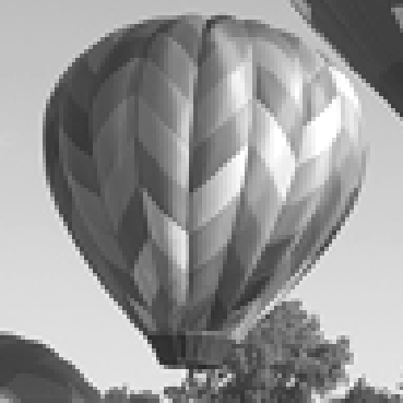
(a) Ground truth

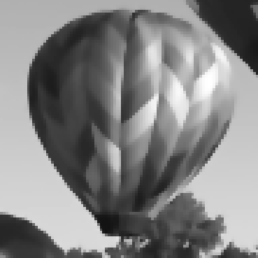
(b) Forward operator

(c) iResNet $\delta=0.01$

(d) iResNet $\delta=0.05$

Linear Blurring

(e) Ground truth

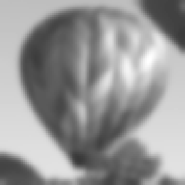
(f) Forward operator

(g) iResNet $\delta=0.01$

(h) iResNet $\delta=0.05$

Figure 10: Comparison of the forward operator (top row: nonlinear diffusion, bottom row: linear blurring) with the trained iResNets for different noise levels. From left to right: Ground truth image, blurred image using the forward operator with no added noise as well as the output (forward pass) of the network trained with Lipschitz parameter $L=0.999$ for noise level $0.01$ and $0.05$.

4.3.1 Directional derivatives and local ill-posedness

(a) $\|\partial_{h}F\|=0.0414$
$\|\partial_{h}\varphi_{\theta}\|=1.27$

(b) $\|\partial_{h}F\|=0.0417$
$\|\partial_{h}\varphi_{\theta}\|=1.24$

(c) $\|\partial_{h}F\|=0.0750$
$\|\partial_{h}\varphi_{\theta}\|=1.00$

(d) $\|\partial_{h}F\|=0.0532$
$\|\partial_{h}\varphi_{\theta}\|=1.18$

(e) $\|\partial_{h}F\|=0.126$
$\|\partial_{h}\varphi_{\theta}\|=0.675$

(f) $\|\partial_{h}F\|=0.165$
$\|\partial_{h}\varphi_{\theta}\|=0.921$

Figure 11: Computation of directions $h$ for which the difference $\|\partial_{h}\varphi_{\theta}(x_{0})\|-\|\partial_{h}F(x_{0})\|$ is particularly large ($\varphi_{\theta}$ trained for the nonlinear diffusion operator with $\delta=0.01$). The direction vector $h$ is displayed in color on the image $x_{0}$ (grayscale). It can be interpreted as a direction in which the network has learned a significant regularization. In the bottom row, $h$ is restricted to the subject of the image $x_{0}$.

Figure 12: Computation of directions $h$ for which the difference $\|\partial_{h}\varphi_{\theta}(x_{0})\|-\|\partial_{h}F(x_{0})\|$ is particularly large ($\varphi_{\theta}$ trained for the nonlinear diffusion operator with different noise levels $\delta$). For the three test images “Balloon”, “Boat” and “Dog”, we display $\|\partial_{h}\varphi_{\theta}(x_{0})\|$ in red and $\|\partial_{h}F(x_{0})\|$ in blue. The dashed lines show the results, where $h$ is restricted to the subject of the image (cf. Figure 12).

A nonlinear inverse problem is called locally ill-posed in a point $x_{0}\in X$, if any open neighborhood of $x_{0}$ contains a sequence $(x_{k})$ such that $F(x_{k})\to F(x_{0})$ but $x_{k}\not\to x_{0}$ [23, Definition 3.15]. For differentiable $F$, this often entails that some directional derivatives $\partial_{h}F(x_{0})=F^{\prime}(x_{0})h$ are small. Accordingly, for our nonlinear diffusion operator $F$ we expect $\|\partial_{h}F(x_{0})\|$ to be small for certain directions $h\in X$, $\|h\|=1$, dependent on the input image $x_{0}\in X$.

In contrast, we expect the trained iResNet $\varphi_{\theta}$ to have learned a regularization for the inverse problem. Thus, we anticipate $\|\partial_{h}\varphi_{\theta}(x_{0})\|\gg\|\partial_{h}F(x_{0})\|$ for the same directions $h$. The Lipschitz constraint even ensures that $\|\partial_{h}\varphi_{\theta}(x_{0})\|\geq 1-L$ is guaranteed. Moreover, we can use gradient ascent to find directions $h\in X$, $\|h\|=1$ such that

$$\|\partial_{h}\varphi_{\theta}(x_{0})\|^{2}-\|\partial_{h}F(x_{0})\|^{2}$$

is as large as possible. In other words, we look for a direction $h$ in which the network has learned the strongest regularization w.r.t. a given input image $x_{0}$. We can also restrict $h$ to certain areas of the image $x_{0}$ in order to analyze the regularization inside this area.

Figure 12 shows the resulting directions $h$ of highest regularization for three different test images $x_{0}$. Note that gradient ascent does not lead to unique solutions and the directions should therefore rather be seen as examples.

The first striking observation is that $h$ consistently exhibits a checkerboard pattern. This occurs because adding a small perturbation $\varepsilon h$ to $x_{0}$ introduces numerous small edges, which are subsequently blurred by the forward operator $F$. Since these small edges may represent important image details, regularization by the iResNet is necessary. Additionally, $h$ is primarily concentrated in the smooth parts of the images, such as the uniform areas of the background. In these regions, the introduction of small edges has the most pronounced effect. Moreover, reconstructing a smooth background without any details is a relatively simple task for a neural network, requiring only few information from the noisy and blurred image $z^{\delta}$ and relying more heavily on the learned prior. Therefore, it is optimal to apply strong regularization in these areas. Even when $h$ is restricted to the subject of the images, it remains concentrated in the smoother regions.

An iResNet trained on higher noise levels is expected to apply a stronger regularization. To verify this, we compare the values of $\|\partial_{h}\varphi_{\theta}(x_{0})\|$ for $\varphi_{\theta}$ trained on different noise levels $\delta$. The result is illustrated in Figure 12. For all three test images, we indeed observe that the amount of regularization increases with $\delta$.

4.3.2 Investigation of the learned forward operator by linearization

In the previous section, we observed that the iResNet has effectively learned to regularize, particularly in smoother regions of the image. In this section, we aim to gain a deeper understanding of this learned regularization by comparing the local behavior of our iResNet $\varphi_{\theta}$ with that of the operator $F$. However, due to the inherent nonlinearity of both the network and the operator, this analysis presents a significant challenge.

To address this challenge, we approximate $\varphi_{\theta}$ and $F$ around a given image $x_{0}\in\mathbb{R}^{n\times m}$ with the help of a first order Taylor expansion. The first order Taylor expansion $T\Psi(\cdot,x_{0}):\mathbb{R}^{n\times m}\to\mathbb{R}^{n\times m}$ of a differentiable operator $\Psi:X\to X$ around $x_{0}$ restricted to some pixel $(n_{0},m_{0})\in\{1,\dots,n\}\times\{1,\dots,m\}$ is given by

$$T\Psi(x,x_{0})\big{|}_{(n_{0},m_{0})}=\Psi(x_{0})\big{|}_{(n_{0},m_{0})}+\left\langle J\Psi(x_{0})\big{|}_{(n_{0},m_{0})},x-x_{0}\right\rangle+R\Psi(x,x_{0})\big{|}_{(n_{0},m_{0})}$$

with Jacobian

$$J\Psi(x_{0})\big{|}_{(n_{0},m_{0})}=\left(\frac{\partial{\Psi}_{n_{0},m_{0}}}{\partial x_{k,l}}(x_{0})\right)_{k=1,\dots,n,\,l=1,\dots,m},$$

$x\in\mathbb{R}^{n\times m}$ and remainder $R\Psi(\cdot,x_{0}):\mathbb{R}^{n\times m}\to\mathbb{R}^{n\times m}$. In the setting of $\Psi$ being our iResNet or the nonlinear diffusion operator, the Jacobian can be interpreted as a linear blurring kernel that approximates the nonlinear diffusion operations of the network and the operator, respectively. This perspective allows us to assign a kernel to each pixel in the image $x_{0}$, providing a visual interpretation of $\varphi_{\theta}$ and $F$. This approach was first introduced in [25] in the context of image classification, leading to the creation of so-called saliency maps, which enable the interpretation of decisions made by image classification networks. While saliency maps in classification tasks are limited to the number of classes, the large number of image pixels in our setting makes manual analysis impractical. To address this, we opted to cluster the kernels of $\varphi_{\theta}$ and $F$ and then analyze the resulting clusters, respectively.

Before discussing the clustering results, we will first provide an overview of our calculation pipeline. The computation of the Jacobians and the clustering is performed separately for each image in the test set. This approach is necessary because we observed that clustering becomes ineffective or fails to converge when the number of pixels exceeds $15\,000$. We found that limiting the number of pixels per image to $1500$ leads to a good trade-off between cluster accuracy and computational efficiency.

We randomly select a set $\mathcal{P}$ of pixel indices, which remains the same across all images, networks and the operator. For each pixel $(n_{0},m_{0})$ in the set $\mathcal{P}$ and fixed image $x_{0}$, we calculate the Jacobians $J\varphi_{\theta}(x_{0})\big{|}_{(n_{0},m_{0})}$ and $JF(x_{0})\big{|}_{(n_{0},m_{0})}$. For the network $\varphi_{\theta}$, this can be achieved efficiently via backpropagation giving access to the gradients of the input image. Each Jacobian is then cropped to a $9\times 9$ region centered around the pixel $(n_{0},m_{0})$. This cropping is performed because pixel values outside this region are typically near zero and do not contain relevant information. In what follows, the cropped image is referred to as the saliency map or linear blurring kernel. Before clustering, we normalize the values of these saliency maps while preserving the sign of the values.

Finally, the transformed saliency maps are clustered using spectral clustering. In addition to spectral clustering, we also evaluated other clustering techniques, ranging from primitive methods to more advanced approaches involving principal component analysis (PCA). However, the clustering results were all very similar, which is why we opted for the standard and straightforward spectral clustering algorithm. This method is particularly effective when the clusters are expected to be highly non-convex. We refer the reader to [28] for a more detailed explanation of spectral clustering.

When applying a clustering method, selecting the number of clusters is a critical hyperparameter that must be determined in advance. Several techniques exist to help identify an appropriate number of clusters. To obtain an initial estimate, we compare the predictions from the elbow method [26], the gap statistic [20], and the gap^∗ statistic [13]. While the elbow method is heuristic in nature, both the gap statistic and the gap^∗ statistic provide a more formal approach grounded in statistical analysis. In the examples presented in this section, we found that using two clusters offers a reasonable trade-off between achieving meaningful data separation and maintaining comparability between the network and the operator.

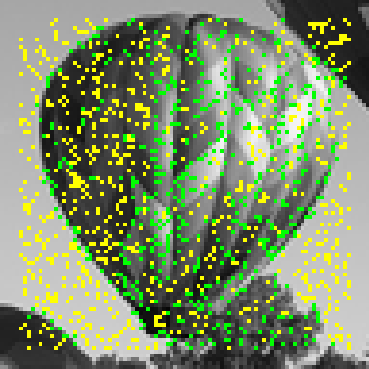
(a) Forward operator

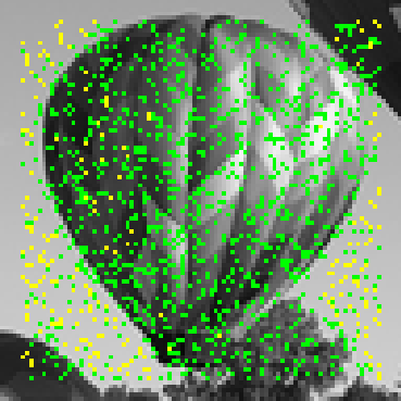
(b) $L=0.999$, $\delta=0.01$

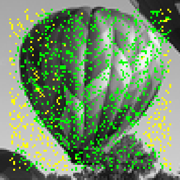
(c) $L=0.999$, $\delta=0.025$

(d) $L=0.999$, $\delta=0.05$

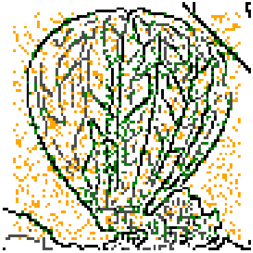
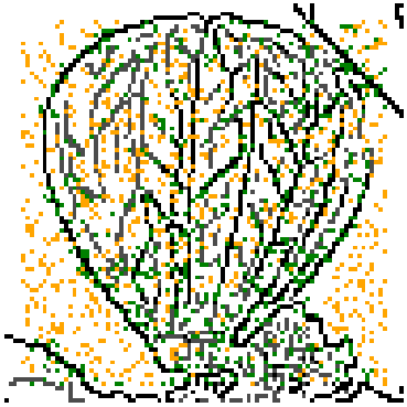
Figure 13: Clustering of the saliency maps of the operator and the network trained with Lipschitz parameter $L=0.999$ for different noise levels. The first row visualizes the clustering with the ground truth image. The second row visualizes the clustering with the edges of the ground truth image. Weak edges are coloured in grey and strong edges are coloured in black.

The clustering results for the operator as well as the network trained with different noise levels and fixed Lipschitz parameter $L=0.999$ are visualized in Figure 13, exemplified on the balloon image from Figure 10. Each pixel for which saliency maps are calculated and clustered is colored based on its cluster assignment. We visualize the results alongside the ground truth image as well as its edges. In all subsequent plots, the cluster with the highest number of pixels that align with the image edges is highlighted in green. The edges are calculated using the Canny edge detection algorithm. We differentiate between weak and strong edges, where strong edges are defined as those whose value exceeds $20\%$ of the maximum of the intermediate edge image generated during the Canny algorithm after applying Sobel filtering and gradient magnitude thresholding.

Figure 13 shows that the operator’s saliency maps are primarily clustered into pixels corresponding to strong edges and those associated with weak edges and smooth areas. In contrast, the clustering for the network trained with $\delta=0.01$ indicates that the saliency maps are very similar for most pixels, as the majority of pixels fall into the cluster visualized in green. This behaviour is less pronounced for the network trained with $\delta=0.025$, where the saliency maps are more distinctly clustered into pixels corresponding to edges and those belonging to smoother regions of the image. The clustering of the network trained with $\delta=0.05$ most closely resembles that of the operator, with weak edges and smooth areas grouped into the same cluster.

Orange cluster

(a) Forward operator

(b) $45\%$ edges

(c) $\boldsymbol{L=0.999}$, $\boldsymbol{\delta=0.01}$

(d) $8\%$ edges

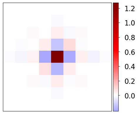
(e) $\boldsymbol{L=0.999}$, $\boldsymbol{\delta=0.025}$

(f) $5\%$ edges

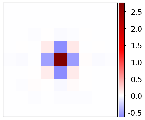
(g) $\boldsymbol{L=0.999}$, $\boldsymbol{\delta=0.05}$

(h) $45\%$ edges

Green cluster

(i) $98\%$ edges

(j) $80\%$ edges

(k) $86\%$ edges

(l) $93\%$ edges

Figure 14: Mean of the saliency maps of the operator and the network trained with Lipschitz parameter $L=0.999$ and noise level $0.01$, $0.025$, $0.05$. The percentage of pixels on edges for each cluster is indicated below each saliency map.

To further investigate the clustering, we visualize the mean saliency maps for the individual clusters of the operator and the network trained with $L=0.999$ for different noise levels in Figure 14. The operator’s mean saliency map of the orange cluster (comprising pixels on weak edges and in smooth areas) is much more spread out compared to that of the green cluster (strong edges). This was to be expected as the strength of the nonlinear diffusion depends on the gradient of the image, with stronger diffusion in areas with smaller gradients.

When comparing the network’s saliency maps to those of the operator, it is particularly striking that the spread of the orange cluster is significantly lower and decreases further as the noise level increases. Since the orange cluster primarily includes pixels in smooth regions and on weak edges, this leads to significantly less blurring in these areas and has a regularizing effect, which is in line with our investigations of the local ill-posedness in the previous section. Additionally, for small noise levels ($\delta=0.01,0.025$), the dispersion of the network’s saliency maps is quite similar across both clusters, which may explain the poor clustering observed in Figure 13.

Furthermore, the network’s mean saliency maps exhibit a strong emphasis on the central pixel, displaying significantly higher values compared to those of the operator. This is particularly the case for the cluster containing pixels in smooth areas as well as high noise levels. To counterbalance this and maintain the range of values in the blurred image, the values of the pixels adjacent to the central pixel are negative.

Overall, the behaviour of the saliency maps leads to an overemphasis of edges and significantly reduced blurring in smooth regions, especially for high noise levels. This aligns with the observations presented in Figure 10.

We also examined the clustering results of the network with varying Lipschitz parameters. Our analysis confirms that smaller Lipschitz parameters significantly reduce the network’s expressiveness, as previously discussed. As a result, the network’s ability to learn an effective regularization from the data is limited for smaller Lipschitz parameters. For the sake of completeness, the results can be found in Appendix B.

So far, the investigations have been based entirely on a single image from the test set, which may lead to biased conclusions. This limitation arises because comparing clustering results across different images, let alone the entire test set, is challenging. Pixel cluster affiliations can vary significantly between different networks and images, making automated comparison difficult. To obtain more reliable results, we decided to manually cluster the pixels of each image in the test set to create comparable clusters. Based on the operator’s behavior and the clustering results of the balloon image, we chose to divide the pixels of each image into two groups: those belonging to smooth areas and those belonging to the edges.

We implement this manual clustering using Canny edge detection to extract the edges of each image in the test set, thereby creating two distinct sets of pixels corresponding to smooth regions and edges. To ensure a clear spatial separation between the two clusters, we dilate the edge image using a $3\times 3$ kernel, assigning pixels to the cluster representing smooth areas only if they are at least two pixels away from an edge. Moreover, the boundary region of the image is excluded from clustering to ensure that the extracted and cropped saliency maps consistently have the same size. For each image in the test set, we then sample $250$ pixels equidistantly from each cluster, calculate the corresponding saliency map, and average them within each cluster.

Smooth Areas

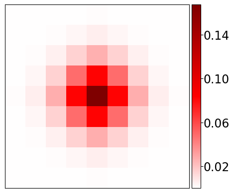
(a) Forward operator

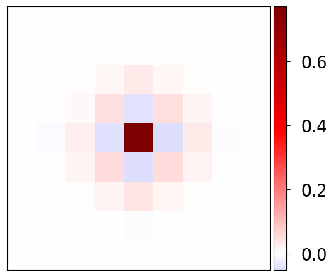
(b) $\boldsymbol{L=0.999}$, $\boldsymbol{\delta=0.01}$

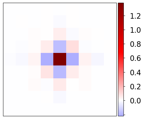
(c) $\boldsymbol{L=0.999}$, $\boldsymbol{\delta=0.025}$

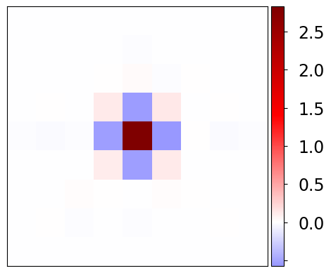
(d) $\boldsymbol{L=0.999}$, $\boldsymbol{\delta=0.05}$

Edges

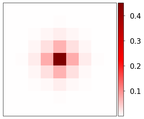
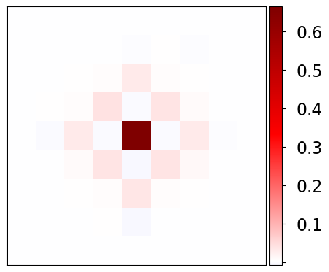
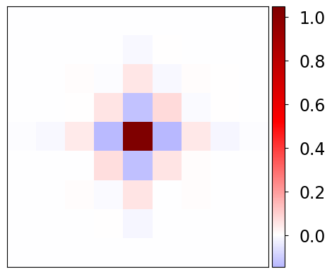
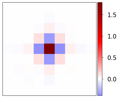
Figure 15: Mean of the saliency maps of the operator and the network trained with Lipschitz parameter $L=0.999$ and noise level $0.01$, $0.025$, $0.05$. The clustering is done manually on the test set according to edge pixels and smooth areas.

The resulting averaged saliency maps are depicted in Figure 15 for the operator as well as the network trained with noise level $\delta=0.01,0.025,0.05$ and Lipschitz parameter $L=0.999$. The mean saliency maps exhibit a behavior remarkably similar to that observed in the clustering of the balloon image. This similarity confirms the reliability and significance of the balloon image’s clustering results, indicating that this behavior generalizes well to other images.

5 Discussion and Outlook

This present work builds on the theoretical foundation of the iResNet reconstruction approach for solving inverse problems, previously introduced in [2, 3], by conducting extensive numerical experiments on two real-world tasks. Our experiments demonstrate the competitiveness of iResNets compared to state-of-the-art reconstruction methods. While the earlier publications [2, 3] established criteria for rendering the iResNet reconstruction approach a convergent regularization scheme, their efficacy in real-world, high-dimensional tasks had not yet been confirmed. To address this, we developed a large-scale iResNet architecture and evaluated its performance on both a linear blurring problem and a nonlinear diffusion problem.

Our results indicate that iResNets perform on par with leading image reconstruction networks, such as U-Nets. However, unlike most state-of-the-art methods, iResNets provide verifiable regularization properties. Specifically, they ensure stability of the resulting reconstruction scheme by controlling the hyperparameter $L$ and offer empirically verifiable convergence to the true solution as the noise level decreases. Additionally, the inherent invertibility of iResNets enables exploration of the learned forward operator. This opens the door to in-depth investigations of the nature of the learned regularization. However, these advantages come at the price of significantly higher training times compared to state-of-the-art methods.

In our numerical experiments, the best trade-off between interpretability of the learned solution and performance was achieved by DiffNets, as introduced in [4], though these are specifically tailored for diffusion problems. In contrast, our iResNet reconstruction approach is applicable to a broader class of inverse problems and offers theoretical guarantees in addition to interpretability. Consequently, to validate the versatility of iResNets, future research should explore their performance across a wider range of forward operators. Furthermore, it is essential to investigate possibilities for reducing the training times of iResNets while preserving their performance in order to increase their efficiency in practical applications.

In summary, this work provides numerical evidence supporting the iResNet regularization scheme as an effective and interpretable learned reconstruction method with theoretical guarantees. Consequently, iResNets offer a promising approach to solving complex real-world inverse problems by bridging the gap between high-performance, data-driven methods that often lack theoretical justification and classical methods with guarantees but inferior performance.

Appendix A Proof of Lemma 3.1

Proof.

Since $g\equiv 1$, $S_{h}u$ fulfills the linear PDE $u=S_{h}u-h\cdot\mathrm{div}(\nabla(S_{h}u))$. It holds

$$\begin{split}\|(Id-S_{h})u\|^{2}&=\|u\|^{2}-2\langle S_{h}u,u\rangle+\|S_{h}u\|^{2}\\ &=\|u\|^{2}-2\langle S_{h}u,S_{h}u-h\cdot\mathrm{div}(\nabla(S_{h}u))\rangle+\|S_{h}u\|^{2}\ \\ &=\|u\|^{2}+2h\langle S_{h}u,\mathrm{div}(\nabla(S_{h}u))\rangle-\|S_{h}u\|^{2}\ .\end{split}$$

Due to the zero Dirichlet or zero Neumann boundary condition on $S_{h}u$, we can go on with

$$\begin{split}\|(Id-S_{h})u\|^{2}&=\|u\|^{2}-2h\langle\nabla(S_{h}u),\nabla(S_{h}u)\rangle-\|S_{h}u\|^{2}\ \\ &\leq\|u\|^{2}-\|S_{h}u\|^{2},\end{split}$$

which completes the proof. ∎

Appendix B Cluster comparison for different Lipschitz parameters

(a) Forward operator

(b) $L=0.95$, $\delta=0.05$

(c) $L=0.99$, $\delta=0.05$

(d) $L=0.999$, $\delta=0.05$

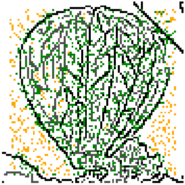
Figure 16: Clustering of the saliency maps of the operator and the network trained with noise level $\delta=0.05$ for different Lipschitz parameters. The first row visualizes the clustering with the ground truth image and the second row with the corresponding edges (weak edges are grey and strong edges are black).

Orange cluster

(a) Forward operator

(b) $45\%$ edges

(c) $\boldsymbol{L=0.95}$, $\boldsymbol{\delta=0.05}$

(d) $5\%$ edges

(e) $\boldsymbol{L=0.99}$, $\boldsymbol{\delta=0.05}$

(f) $2\%$ edges

(g) $\boldsymbol{L=0.999}$, $\boldsymbol{\delta=0.05}$

(h) $45\%$ edges

Green cluster

(i) $98\%$ edges

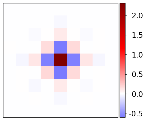
(j) $88\%$ edges

(k) $87\%$ edges

(l) $93\%$ edges

Figure 17: Mean of the saliency maps of the operator and the network trained with Lipschitz parameters $L=0.95,0.99,0.999$ and noise level $0.05$. The percentage of pixels on edges for each cluster is indicated below each saliency map.

References

- [1] A. Y. N. Adam Coates, Honglak Lee. An analysis of single layer networks in unsupervised feature learning. In Proceedings of the 14th International Conference on Artificial Intelligence and Statistics (AISTATS), 2011.
- [2] C. Arndt, A. Denker, S. Dittmer, N. Heilenkötter, M. Iske, T. Kluth, P. Maass, and J. Nickel. Invertible residual networks in the context of regularization theory for linear inverse problems. Inverse Problems, 39(12):125018, nov 2023.
- [3] C. Arndt, S. Dittmer, N. Heilenkötter, M. Iske, T. Kluth, and J. Nickel. Bayesian view on the training of invertible residual networks for solving linear inverse problems. Inverse Problems, 40(4):045021, mar 2024.
- [4] S. Arridge and A. Hauptmann. Networks for nonlinear diffusion problems in imaging. Journal of Mathematical Imaging and Vision, 62:471–487, 2020.
- [5] S. Bai, J. Z. Kolter, and V. Koltun. Deep equilibrium models. In H. Wallach, H. Larochelle, A. Beygelzimer, F. d'Alché-Buc, E. Fox, and R. Garnett, editors, Advances in Neural Information Processing Systems, volume 32. Curran Associates, Inc., 2019.
- [6] J. Behrmann, W. Grathwohl, R. T. Chen, D. Duvenaud, and J.-H. Jacobsen. Invertible residual networks. In International Conference on Machine Learning, pages 573–582. PMLR, 2019.
- [7] M. Benning and M. Burger. Modern regularization methods for inverse problems. Acta Numerica, 27:1–111, 2018.
- [8] L. Bungert, R. Raab, T. Roith, L. Schwinn, and D. Tenbrinck. Clip: Cheap lipschitz training of neural networks. In A. Elmoataz, J. Fadili, Y. Quéau, J. Rabin, and L. Simon, editors, Scale Space and Variational Methods in Computer Vision, pages 307–319, Cham, 2021. Springer International Publishing.
- [9] H. W. Engl, M. Hanke, and A. Neubauer. Regularization of Inverse Problems. Springer Dordrecht, 1st edition, 2000.
- [10] D. Gilton, G. Ongie, and R. M. Willett. Deep equilibrium architectures for inverse problems in imaging. IEEE Transactions on Computational Imaging, 7:1123–1133, 2021.
- [11] J. Hertrich. Proximal residual flows for bayesian inverse problems. In L. Calatroni, M. Donatelli, S. Morigi, M. Prato, and M. Santacesaria, editors, Scale Space and Variational Methods in Computer Vision, pages 210–222, Cham, 2023. Springer International Publishing.
- [12] B. Hofmann, B. Kaltenbacher, C. Pöschl, and O. Scherzer. A convergence rates result for Tikhonov regularization in Banach spaces with non-smooth operators. Inverse Problems, 23(3):987–1010, 2007.
- [13] M. Mohajer, K.-H. Englmeier, and V. J. Schmid. A comparison of gap statistic definitions with and without logarithm function. Department of Statistics: Technical Reports, 96, 2010.
- [14] V. Monga, Y. Li, and Y. C. Eldar. Algorithm unrolling: Interpretable, efficient deep learning for signal and image processing. IEEE Signal Processing Magazine, 38(2):18–44, 2021.
- [15] S. Mukherjee, S. Dittmer, Z. Shumaylov, S. Lunz, O. Öktem, and C.-B. Schönlieb. Learned convex regularizers for inverse problems. Preprint, arXiv:2008.02839, 2021.
- [16] S. Mukherjee, A. Hauptmann, O. Öktem, M. Pereyra, and C.-B. Schönlieb. Learned reconstruction methods with convergence guarantees: A survey of concepts and applications. IEEE Signal Processing Magazine, 40(1):164–182, 2023.
- [17] S. Mukherjee, C.-B. Schönlieb, and M. Burger. Learning convex regularizers satisfying the variational source condition for inverse problems. In NeurIPS 2021 Workshop on Deep Learning and Inverse Problems, 2021.
- [18] D. Obmann and M. Haltmeier. Convergence analysis of equilibrium methods for inverse problems. arXiv preprint arXiv:2306.01421, 2023.
- [19] P. Perona and J. Malik. Scale-space and edge detection using anisotropic diffusion. IEEE Transactions on Pattern Analysis and Machine Intelligence, 12(7):629–639, 1990.
- [20] T. H. Robert Tibshirani, Guenther Walther. Estimating the number of clusters in a data set via the gap statistic. Journal of the Royal Statistical Society Series B: Statistical Methodology, 63:411–423, 2001.
- [21] O. Ronneberger, P. Fischer, and T. Brox. U-Net: Convolutional networks for biomedical image segmentation. In N. Navab, J. Hornegger, W. M. Wells, and A. F. Frangi, editors, Medical Image Computing and Computer-Assisted Intervention - MICCAI 2015, volume 9351, pages 234–241, 2015.
- [22] L. Ruthotto and E. Haber. Deep neural networks motivated by partial differential equations. Journal of Mathematical Imaging and Vision, 62:352–364, 2020.
- [23] T. Schuster, B. Kaltenbacher, B. Hofmann, and K. S. Kazimierski. Regularization Methods in Banach Spaces. De Gruyter, Berlin, Boston, 2012.
- [24] F. Sherry, E. Celledoni, M. J. Ehrhardt, D. Murari, B. Owren, and C.-B. Schönlieb. Designing stable neural networks using convex analysis and odes. Physica D: Nonlinear Phenomena, 463:134159, 2024.
- [25] K. Simonyan, A. Vedaldi, and A. Zisserman. Deep inside convolutional networks: Visualising image classification models and saliency maps, 2014.
- [26] R. Thorndike. Who belongs in the family? Psychometrika, 18(4):267–276, 1953.
- [27] S. V. Venkatakrishnan, C. A. Bouman, and B. Wohlberg. Plug-and-play priors for model based reconstruction. In 2013 IEEE Global Conference on Signal and Information Processing, pages 945–948, 2013.
- [28] U. von Luxburg. A tutorial on spectral clustering. Statistics and Computing, 17:395–416, 2007.