A Plug-and-Play Method for Guided Multi-contrast MRI Reconstruction based on Content/Style Modeling

Abstract

Since multiple MRI contrasts of the same anatomy contain redundant information, one contrast can be used as a prior for guiding the reconstruction of an undersampled subsequent contrast. To this end, several learning-based guided reconstruction methods have been proposed. However, two key challenges remain – (a) the requirement of large paired training datasets and (b) the lack of intuitive understanding of the model’s internal representation and utilization of the shared information. We propose a modular two-stage approach for guided reconstruction, addressing these challenges. A content/style model of two-contrast image data is learned in a largely unpaired manner and is subsequently applied as a plug-and-play operator in iterative reconstruction. The disentanglement of content and style allows explicit representation of contrast-independent and contrast-specific factors. Based on this, incorporating prior information into the reconstruction reduces to simply replacing the aliased reconstruction content with clean content derived from the reference scan. We name this novel approach PnP-MUNIT. Various aspects like interpretability and convergence are explored via simulations. Furthermore, its practicality is demonstrated on the NYU fastMRI DICOM dataset and two in-house raw datasets, obtaining up to 32.6% more acceleration over learning-based non-guided reconstruction for a given SSIM. In a radiological task, PnP-MUNIT allowed 33.3% more acceleration over clinical reconstruction at diagnostic quality.

I Introduction

Magnetic resonance imaging (MRI) is an invaluable medical imaging modality due to the high-quality scans it delivers, the variety of complementary information it can capture, and its lack of radiation-related risks, leading to its wide usage in clinical practice. However, its central limitation is the inherently slow data acquisition process. The raw sensor data is acquired in the frequency domain, or k-space, from which the image is reconstructed. Over the last 25 years, advancements such as parallel imaging [1, 2], compressed sensing (CS) [3], and deep learning reconstruction [4] have enabled considerable speedups by allowing sub-Nyquist k-space sampling and relying on computationally sophisticated reconstruction. These techniques have subsequently been implemented on commercial MRI systems and have demonstrated (potential) improvements in clinical workflow [5].

A clinical MRI session typically involves the acquisition of multiple scans of the same anatomy through the application of different MR pulse sequences and thus exhibiting different contrasts. Because these scans are different reflections of the same underlying reality, they share a high degree of shared structure. However, currently deployed clinical protocols acquire and reconstruct each scan as an independent measurement, not leveraging the information redundancy across scans. There is, therefore, an opportunity to further optimize MRI sessions by exploiting this shared information. On the reconstruction side, multi-contrast methods have addressed this problem by introducing the shared information into the reconstruction phase to allow higher levels of k-space undersampling. In the simplest case of two contrasts, multi-contrast reconstruction can be classified into two types – (a) guided reconstruction, where an existing high-quality reference scan is used to guide the reconstruction of an undersampled second scan [6, 7, 8] and (b) joint reconstruction, where both contrasts are undersampled and are reconstructed simultaneously [9, 10, 11]. In this work, we consider the problem of guided reconstruction, assuming no inter-scan motion between the reference scan and the reconstruction.

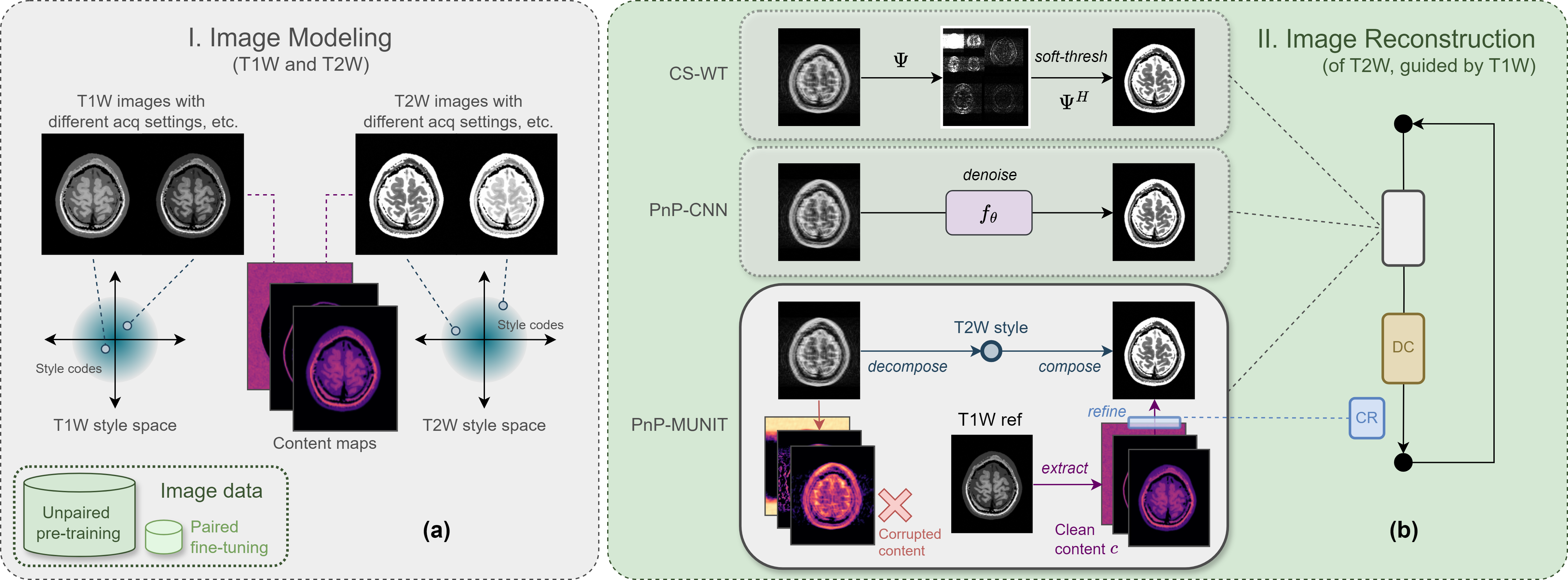
Figure 1: Our two-stage approach to guided reconstruction. (a) The first stage learns a content/style model of two-contrast MR image data in a largely unpaired manner. (b) The reconstruction stage applies this model as a content restoration operator (bottom) within an ISTA-based iterative algorithm, namely PnP-MUNIT. Guidance from the reference is introduced into the reconstruction by simply replacing its aliased content with clean content $c$ derived from the reference. CR denotes a content refinement update, which iteratively corrects for inconsistencies between the reference content and the measured k-space data, improving the effectiveness of the content restoration operator. DC denotes data consistency. Wavelet-domain soft-thresholding (top) and CNN-based denoising (middle) used in CS and PnP reconstructions, respectively, are shown for comparison.

The guided reconstruction problem entails using the spatial structure of the reference scan as a prior to complement the undersampled k-space measurements of the target scan. This problem has been formulated in different ways, ranging from conventional CS [6, 7] to end-to-end learning with unrolled networks [8, 12, 13] and, more recently, diffusion model-based Bayesian maximum a posteriori estimation [14]. Most learning-based approaches, although more powerful than earlier hand-crafted ones, suffer from two main limitations: (a) requirement of large paired training dataset, limiting the effective usage of real-world clinical MR data, and (b) lack of insight into the representation and utilization of the shared underlying structure. We address both issues, leveraging ideas from image-to-image modeling, content/style decomposition, and plug-and-play reconstruction. To the best of our knowledge, ours is the first work that deeply explores content/style modeling for multi-contrast MRI reconstruction.

In recent years, image-to-image translation has found application in the direct estimation of one MR contrast from another [15, 16, 17]. Viewed in the light of MR physics, cross-contrast translation takes an extreme stance by completely ignoring fundamental differences in contrast-specific sensitivities and relying solely on the prior contrast. Cross-contrast translation, by itself, is not a practically reliable solution because data acquisition is necessary for obtaining new information about the anatomy. That said, literature on unpaired image translation provides a repertoire of useful tools such as joint generative modeling of two-domain image data [18, 19], which can be adopted to complement image reconstruction. We observe that methods such as MUNIT [19] can be applied to learn semantically meaningful representations of contrast-independent and contrast-specific information as content and style, respectively, without the need for spatially aligned paired training data.

Plug-and-play (PnP) methods are an emerging paradigm for solving inverse problems in computational imaging. The main research line [20, 21] has focused on learning CNN-based denoising models and applying them as functions replacing proximal operators in iterative algorithms like ISTA and ADMM, demonstrating improved image recovery. An advantage of this approach is the decoupling of the learning problem of image modeling from the inverse problem of image reconstruction, thereby simplifying model training and improving generalizability across different acceleration factors, undersampling patterns, etc. With this design pattern in mind, we combine content/style image modeling and iterative reconstruction in a PnP-like framework.

We propose a two-stage approach for guided reconstruction. We first leverage semantic content/style modeling to learn explicit representations of contrast-independent and contrast-specific components from two-contrast MR image data. This learned model is subsequently embedded into an iterative reconstruction framework resulting in a content/style-based PnP-like algorithm [22]. An overview of our approach is shown in Fig. 1. Specifically, our contributions are four-fold:

1. We show that unpaired training can be used to disentangle contrast-independent and contrast-specific information as content and style, respectively, followed by a fine-tuning strategy to refine the content representation using a modest amount of paired data.

2. With this content/style model as the basis, we define a content restoration operator capable of removing severe undersampling artifacts from the reconstruction image given the corresponding reference image.

3. Developing this idea further, we propose PnP-MUNIT, a modular algorithm for guided reconstruction, combining the flexibility of the plug-and-play approach with the semantic interpretability of content/style decomposition.

4. Through comprehensive experimentation, we shed light on several properties of PnP-MUNIT such as interpretability and convergence as well as demonstrating its applicability on real-world raw data and its potential clinical utility for a specific radiological task.

II Related Work

II-A Reconstruction Methods for Accelerated MRI

Techniques for accelerating MRI by k-space undersampling go back to compressed sensing (CS) [3], which combines random sampling with sparsity-based iterative denoising, most commonly implemented based on the ISTA [23] or ADMM [24] family of algorithms. Most modern deep learning-based reconstruction methods focus on improving the denoising part. Plug-and-play (PnP) methods [20, 21] replace the proximal operator in ISTA and ADMM with off-the-shelf denoisers such as a learned convolutional denoising model. Unrolled networks [25, 26, 4] extend this idea by casting the entire iterative algorithm into one large network, trained end-to-end. This makes them more adaptive to factors such as sampling pattern and acceleration, although at a cost of generalizability [20].

One of the earliest CS-based guided reconstruction methods was proposed by Ehrhardt and Betcke [6] introducing structure-guided total variation (STV), which assumes the sparse coefficients of the reconstruction to be partially known based on edge features in the reference scan. On the other hand, unrolled network-based guided methods [8, 12, 27, 28] supply the reference scan as an additional input to the reconstruction model allowing it to automatically learn the suitable features to extract and transfer into the reconstruction, and have proved to be more effective than conventional algorithms. However, they suffer from two issues limiting their practicality. First, they require large paired training datasets, which is too strong a constraint when working with retrospectively collected clinical data which reflects the natural inconsistencies of routine practice such as missing contrasts, differences in spatial resolutions, and the existence of inter-scan motion. Second, most of these methods neither explicitly represent the prior information nor provide a clear mechanism by which it is incorporated into the reconstruction. On the other hand, a conventional CS approach like STV precisely defines the prior information and the guidance mechanism. A reconstruction method combining this form of transparency with the effectiveness of deep learning-based methods, while maintaining lenient data requirement, is still needed.

II-B Unpaired Image-to-Image Modeling

Image-to-image modeling is the general problem of learning a mapping between two image domains and was first addressed by Pix2Pix [29] and CycleGAN [30] in paired and unpaired settings, respectively. Another line of unpaired image translation methods, the first of which was UNIT [18], assumes a shared latent space underlying the two domains to explicitly represent shared information, thereby making it more interpretable than CycleGAN which directly models the image-to-image mapping. However, both assume a deterministic one-to-one mapping between the two domains, ignoring the fact that an image in one domain can have multiple valid renderings in the other. Deterministic image translation has been widely applied to MRI contrast-to-contrast synthesis [15, 31, 16]. However, they fundamentally do not account for the variability of the scanning setup which influence the realized contrast level and the differential visibility of pathologies in the target image. Denck et al. [17] partially address this problem by proposing contrast-aware MR image translation where the acquisition sequence parameters are fed into the network to control the output’s contrast level. However, this model is too restrictive since it assumes a single pre-defined mode of variability (i.e. global contrast level) in the data, for which the labels (i.e. sequence parameters) must be available.

MUNIT [19] extended UNIT by modeling domain-specific variability in addition to domain-independent structure, overcoming the deterministic mapping limitation of UNIT. The result was a stochastic image translation model which, given an input image, generates a distribution of synthetic images sharing the same “content” but differing in “style”. Clinical MR images of a given protocol contain multiple modes of variability, many of which are not known a priori. We argue that MUNIT, due to the minimal assumptions it makes, can be generally applied to learn domain-independent anatomical structure and domain-specific variability from an unpaired multi-contrast dataset as content and style, respectively.

II-C Combining Image Translation with Reconstruction

Acknowledging the fundamental limitations of MR contrast prediction, some prior work has attempted combining it with multi-contrast reconstruction. A naive form of guided reconstruction involves generating a synthetic image from the reference scan via deterministic image translation and using it in L2-regularized classical reconstruction [32]. More recent work by Xuan et al. [33] proposes a joint image translation and reconstruction method based on optimal transport which additionally accounts for misalignment between the reference and reconstruction images. Levac et al. [14] formulate guided reconstruction as a highly general Bayesian maximum a posteriori estimation problem and solve it iteratively via Langevin update steps, using an image-domain diffusion model as the score function of the prior distribution. While these are promising directions, an alternative general approach leveraging semantic content/style modeling in multi-contrast reconstruction could potentially provide a connection with the well-established MR physics concepts of quantitative tissue maps, acquisition parameters, and physical models. Such an interpretable and unifying approach remains to be found.

III Methods

III-A Reconstruction Problem

III-A1 Undersampled MRI reconstruction

Given a set of $P$ acquired k-space samples $y\in\mathbb{C}^{P}$ and the MRI forward operator $A\in\mathbb{C}^{P\times Q}$, CS reconstruction of the image $x\in\mathbb{C}^{Q}$ with $Q$ voxels is given as

$$\min_{x}||Ax-y||_{2}^{2}+\lambda||\Psi x||_{1},$$ (1)

where $\Psi$ is some sparsifying transform (e.g. wavelet) and $\lambda$ is the regularization strength. A commonly used algorithm to solve this optimization problem is ISTA, which iteratively applies the following two update steps:

$$r^{k}\leftarrow\Psi^{H}\mathrm{soft}(\Psi x^{k-1};\lambda),$$ (2)

$$x^{k}\leftarrow r^{k}-\eta A^{H}(Ar^{k}-y).$$ (3)

Eq. (2) performs soft-thresholding in the transform domain, thereby reducing the incoherent undersampling artifacts in image $x^{k-1}$, whereas (3) enforces soft data consistency on image $r^{k}$ by taking a single gradient descent step over the least-squares term, controlled by step size $\eta$.

III-A2 Plug-and-play denoiser

Plug-and-play methods replace the analytical operation of (2) with off-the-shelf denoisers. A CNN-based denoiser is of special interest as it incorporates a learning-based component into iterative reconstruction. Given a CNN model $f_{\theta}$ trained to remove i.i.d. Gaussian noise from an image, PnP-CNN [20] modifies Eq. (2) to

$$r^{k}\leftarrow f_{\theta}(x^{k-1}).$$ (4)

III-A3 Plug-and-play content restoration operator

In guided reconstruction, a spatially aligned reference $x^{\mathrm{ref}}_{1}$ is available, which captures the same underlying semantic content as the reconstruction image. Inspired by the PnP design, we cast the problem of incorporating prior information from $x^{\mathrm{ref}}_{1}$ into reconstruction $x_{2}^{k-1}$ as the restoration of its semantic content, which has been corrupted by undersampling. We propose a content restoration operator $g_{M}(.;c)$ such that (2) becomes

$$r_{2}^{k}\leftarrow g_{M}(x_{2}^{k-1};c),$$ (5)

where a content/style model $M$ is used to decompose $x_{2}^{k-1}$ into content and style, followed by a replacement of this content with clean content $c$ derived from $x^{\mathrm{ref}}_{1}$ and composing the image $r_{2}^{k}$ from it. Before formally defining this operator and developing the reconstruction algorithm, we discuss the steps required to learn the content/style model $M$.

III-B Content/Style Modeling

Given an image dataset of two MR contrasts we make the general assumption that there exists an underlying contrast-independent spatial structure which, influenced by arbitrary contrast-specific factors, is rendered as the contrast images.

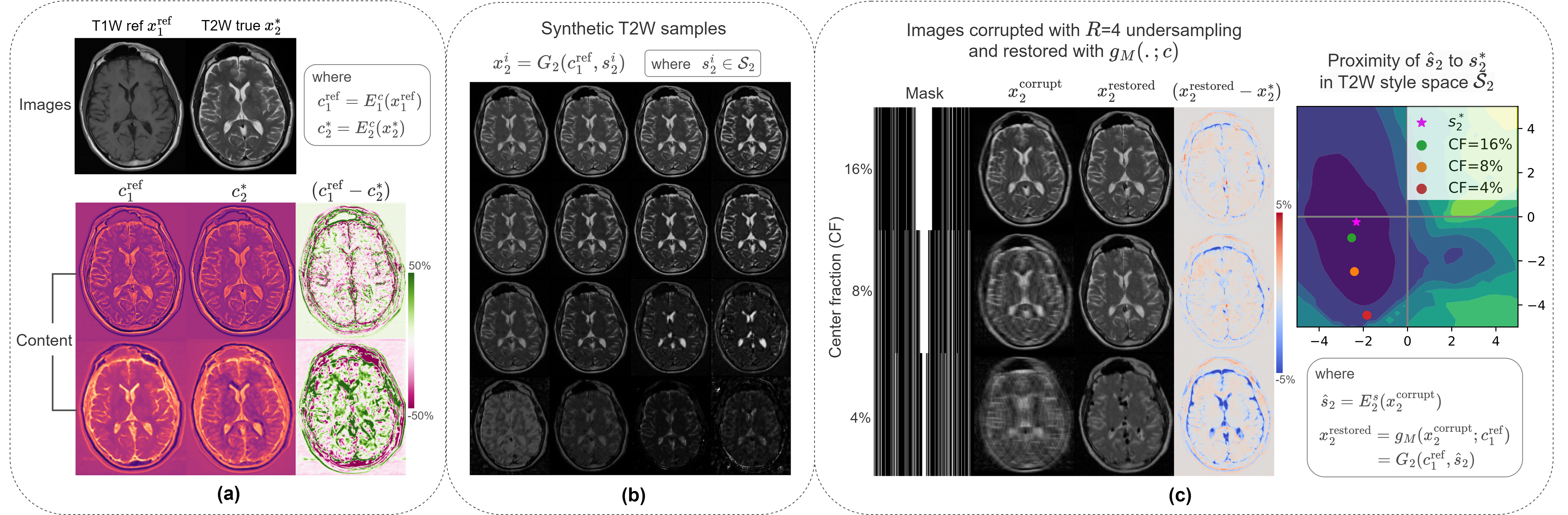
Figure 2: A trained content/style model $M$ and the content restoration operator $g_{M}(.;c)$ based on it. (a) T1W/T2W pair and corresponding content maps. Despite general agreement between their content, there is notable discrepancy. (b) Synthetic T2W images generated from 16 style codes grid-sampled from $\mathcal{S}_{2}$, showing a smooth variation in image contrast and a roughly constant anatomical structure. (c) $g_{M}(.;c)$ is applied on 3 cases where $x_{2}^{*}$ was corrupted with $R$=4 undersampling with different center fractions. Sampling more low-frequency lines leads to more accurate style estimate $\hat{s}_{2}$ and thus better image $x_{2}^{\mathrm{restored}}$. Contours in $\mathcal{S}_{2}$ indicate the mean absolute error of the synthetic images from that region.

III-B1 Unpaired pre-training of MUNIT

We formulate our content/style model based on the MUNIT framework [19]. We define “domain” as the set $\mathcal{X}_{i}$ of images of a certain contrast comprising the dataset, where $i\in\{1,2\}$. “Content” $c\in\mathcal{C}$ is defined here as the underlying contrast-independent structure and is represented as a set of spatial maps, whereas “style” $s_{i}\in\mathcal{S}_{i}$ corresponds to the various modes of variability in one domain which cannot be explained by the other, e.g. global effects of acquisition settings, contrast-specific tissue features, etc, and is thus represented as a low-dimensional vector. MUNIT posits the existence of functions $G_{i}^{*}:\mathcal{C}\times\mathcal{S}_{i}\rightarrow\mathcal{X}_{i}$ and their inverses $E_{i}^{*}=(G_{i}^{*})^{-1}$, and learns them jointly via unpaired training given samples from marginal distributions $p(x_{i})$. In practice, the encoder $E_{i}$ is split into content encoder $E_{i}^{c}$ and style encoder $E_{i}^{s}$. Thus, the content/style model is specified as $M=\{E_{1}^{c},E_{2}^{c},E_{1}^{s},E_{2}^{s},G_{1},G_{2}\}$.

The MUNIT loss function comprises of 4 terms:

$$\mathcal{L_{\mathrm{MUNIT}}}=\mathcal{L}_{\mathrm{GAN}}+\alpha_{1}\mathcal{L}_{\mathrm{image}}^{\mathrm{self}}+\alpha_{2}\mathcal{L}_{\mathrm{content}}^{\mathrm{self}}+\alpha_{3}\mathcal{L}_{\mathrm{style}}^{\mathrm{self}},$$ (6)

where

$$\begin{split}\mathcal{L}_{\mathrm{GAN}}=\>&\mathbb{E}_{x_{1}\sim p(x_{1}),s_{2}\sim q(s_{2})}[(1-D_{2}(G_{2}(E_{1}^{c}(x_{1}),s_{2})))^{2}]+\\ &\mathbb{E}_{x_{2}\sim p(x_{2}),s_{1}\sim q(s_{1})}[(1-D_{1}(G_{1}(E_{2}^{c}(x_{2}),s_{1})))^{2}],\end{split}$$ (7)

$$\begin{split}\mathcal{L}_{\mathrm{image}}^{\mathrm{self}}=\>&\mathbb{E}_{x_{1}\sim p(x_{1})}[||x_{1}-G_{1}(E_{1}^{c}(x_{1}),E_{1}^{s}(x_{1}))||_{1}]+\\ &\mathbb{E}_{x_{2}\sim p(x_{2})}[||x_{2}-G_{2}(E_{2}^{c}(x_{2}),E_{2}^{s}(x_{2}))||_{1}],\end{split}$$ (8)

$$\begin{split}\mathcal{L}_{\mathrm{content}}^{\mathrm{self}}=\>&\mathbb{E}_{c_{1}\sim p(c_{1}),s_{2}\sim q(s_{2})}[||c_{1}-E_{1}^{c}(G_{2}(c_{1},s_{2}))||_{1}]+\\ &\mathbb{E}_{c_{2}\sim p(c_{2}),s_{1}\sim q(s_{1})}[||c_{2}-E_{2}^{c}(G_{1}(c_{2},s_{1}))||_{1}],\end{split}$$ (9)

$$\begin{split}\mathcal{L}_{\mathrm{style}}^{\mathrm{self}}=\>&\mathbb{E}_{c_{1}\sim p(c_{1}),s_{2}\sim q(s_{2})}[||s_{2}-E_{2}^{s}(G_{2}(c_{1},s_{2}))||_{1}]+\\ &\mathbb{E}_{c_{2}\sim p(c_{2}),s_{1}\sim q(s_{1})}[||s_{1}-E_{1}^{s}(G_{1}(c_{2},s_{1}))||_{1}].\end{split}$$ (10)

$\mathcal{L}_{\mathrm{image}}^{\mathrm{self}}$ is the autoencoder image recovery loss, which promotes preservation of input information in the latent space. $\mathcal{L}_{\mathrm{content}}^{\mathrm{self}}$ and $\mathcal{L}_{\mathrm{style}}^{\mathrm{self}}$ are the content and style recovery losses, respectively, which specialize parts of the latent code into content and style components. $\mathcal{L}_{\mathrm{GAN}}$ is the adversarial loss, which enables unpaired training by enforcing distribution-level similarity between synthetic and real images via discriminators $D_{1}$ and $D_{2}$. $\alpha_{1}$, $\alpha_{2}$, and $\alpha_{3}$ are hyperparameters.

III-B2 Paired fine-tuning

While the pre-training stage learns useful content/style representations, the model can be adapted to our task by improving its content preservation. To this end, we propose a paired fine-tuning (PFT) stage, leveraging a modest amount of paired data. Given samples from the joint distribution $p(x_{1},x_{2})$, our fine-tuning objective is given as

$$\mathcal{L}_{\mathrm{PFT}}=\mathcal{L}_{\mathrm{GAN}}+\beta_{1}\mathcal{L}_{\mathrm{image}}^{\mathrm{self}}+\beta_{2}\mathcal{L}_{\mathrm{image}}^{\mathrm{cross}}+\beta_{3}\mathcal{L}_{\mathrm{content}}^{\mathrm{cross}},$$ (11)

where

$$\begin{split}\mathcal{L}_{\mathrm{image}}^{\mathrm{cross}}=\>&\mathbb{E}_{\{x_{1},x_{2}\}\sim p(x_{1},x_{2})}[\\ &||x_{2}-G_{2}(E_{1}^{c}(x_{1}),E_{2}^{s}(x_{2}))||_{1}+\\ &||x_{1}-G_{1}(E_{2}^{c}(x_{2}),E_{1}^{s}(x_{1}))||_{1}],\end{split}$$ (12)

$$\begin{split}\mathcal{L}_{\mathrm{content}}^{\mathrm{cross}}=\mathbb{E}_{\{x_{1},x_{2}\}\sim p(x_{1},x_{2})}[||E_{1}^{c}(x_{1})-E_{2}^{c}(x_{2})||_{1}].\end{split}$$ (13)

$\mathcal{L}_{\mathrm{image}}^{\mathrm{cross}}$ is a pixel-wise image translation loss, which provides image-level supervision, and $\mathcal{L}_{\mathrm{content}}^{\mathrm{cross}}$ is a paired content loss, which penalizes discrepancy between the contents. $\beta_{1}$, $\beta_{2}$, and $\beta_{3}$ are an additional set of hyperparameters.

III-B3 Network architecture and locality bias

Following the original paper [19], our content encoders $E_{i}^{c}$ consist of an input convolutional layer potentially followed by strided downsampling convolutions, and finally a series of residual blocks. Style encoders $E_{i}^{s}$ consist of input and downsampling convolutions followed by adaptive average pooling and a fully-connected layer that outputs the latent vector. Decoders $G_{i}$ follow a similar structure as the content encoders except in reverse. Style is introduced into the decoder via AdaIN operations which modulate the activation maps derived from the content. We note that in this architecture, the content-size-to-image-size ratio reflects the level of spatial structure one expects to be shared between the two domains. This (relative) content size is thus an inductive bias, known as the locality bias [34], built into the model. A model with high locality bias has a large content size, allowing for a richer content that strongly influences the output’s spatial structure, while simultaneously restricting style to learn low-level global features.

III-C Iterative Reconstruction with Content Consistency

Given the content/style model $M$, we consider $\mathcal{X}_{1}$ and $\mathcal{X}_{2}$ as reference and target domains, respectively and define the content restoration operator $g_{M}(.;c)$ as

$$x^{\mathrm{restored}}_{2}=g_{M}(x^{\mathrm{corrupt}}_{2};c_{1}^{\mathrm{ref}}):=G_{2}(c_{1}^{\mathrm{ref}},E^{s}_{2}(x^{\mathrm{corrupt}}_{2})),$$ (14)

where $x^{\mathrm{corrupt}}_{2}$ is the reconstruction corrupted with undersampling artifacts, $x^{\mathrm{restored}}_{2}$ is the restored image, and content $c_{1}^{\mathrm{ref}}=E^{c}_{1}(x^{\mathrm{ref}}_{1})$. This operation restores $x^{\mathrm{corrupt}}_{2}$ by simply replacing its aliased content with the clean content from $x^{\mathrm{ref}}_{1}$, a rule which will later be softened with (15).

Note that this is a radical operation as it discards all structure contained in $x^{\mathrm{corrupt}}_{2}$, retaining only a compact style code $\hat{s}_{2}=E_{2}^{s}(x^{\mathrm{corrupt}}_{2})$. Let $x_{2}^{*}$ be the ground truth reconstruction with content $c_{2}^{*}$ and style $s_{2}^{*}$. The success of the content restoration operation depends on two conditions – (a) $c_{1}^{\mathrm{ref}}$ is close to $c_{2}^{*}$ and (b) $\hat{s}_{2}$ is close to $s_{2}^{*}$. The first condition is roughly satisfied because the model is explicitly trained to minimize content discrepancy, which can be seen in Fig. 2a, but more on this later. On the other hand, it is not obvious that the second condition should hold too and hence deserves a closer look. Assuming a high degree of shared spatial structure between the two domains, the optimal model has high locality bias (based on Section III-B3). Thus, style represents low-level global image features, e.g. contrast variations, as observed in Fig. 2b. It is a well known fact that image contrast is contained prominently in the center of the k-space. Hence, the estimate $\hat{s}_{2}$ can be made arbitrarily close to $s_{2}^{*}$ by sufficiently sampling the k-space center, as shown empirically in Fig. 2c.

Algorithm 1 PnP-MUNIT

1:$y$, $A$, $x^{\mathrm{ref}}_{1}$, $M$, $\eta$, $\gamma$ $\triangleright$ where $M=\{E_{1}^{c},E_{1}^{s},E_{2}^{c},E_{2}^{s},G_{1},G_{2}\}$

2:$k\leftarrow 0$

3:$x_{2}^{k}\leftarrow A^{H}y$

4:$c^{k}\leftarrow E_{1}^{c}(x^{\mathrm{ref}}_{1})$

5:repeat

6:     $k\leftarrow k+1$

7:     $r_{2}^{k}\leftarrow g_{M}(x_{2}^{k-1};c^{k-1})$ $\triangleright$ Content consistency

8:     $x_{2}^{k}\leftarrow r_{2}^{k}-\eta A^{H}(Ar_{2}^{k}-y)$ $\triangleright$ Data consistency

9:     $c^{k}\leftarrow c^{k-1}-\gamma\nabla_{c}||AG_{2}(c^{k-1},E_{2}^{s}(x_{2}^{k}))-y||_{2}^{2}$ $\triangleright$ CR

10:until convergence

11:return $x_{2}^{k}$

Applying data consistency update (3) following $g_{M}(.;c)$ in repetition yields an iterative scheme, where the latter can be viewed as a hard content consistency update. Fig. 2a shows that although $c_{1}^{\mathrm{ref}}$ and $c_{2}^{*}$ are roughly similar, there is notable discrepancy between them. There are at least two possible sources of content discrepancy, which make this phenomenon inevitable – (a) model-related, e.g. practical issues like sub-optimal training or fundamental limits such as irreducible error, and (b) reference image-related, e.g. presence of artifacts independent of the reconstruction. During reconstruction, a $c_{1}^{\mathrm{ref}}$ that conflicts with $c_{2}^{*}$, and with k-space $y$ by extension, would hamper convergence. While model-related discrepancy is partly tackled by the PFT strategy (Section III-B2), we propose a content refinement (CR) step to correct for the remaining discrepancy in the reconstruction stage. The content state is initialized with $c_{1}^{\mathrm{ref}}$ and gradually refined to be consistent with the acquired k-space $y$ as

$$c^{k}\leftarrow c^{k-1}-\gamma\nabla_{c}||AG_{2}(c^{k-1},E_{2}^{s}(x_{2}^{k}))-y||_{2}^{2},$$ (15)

where $\gamma$ is the step size. This update equation mirrors the form of the data consistency update (3), except here the gradient is taken with respect to content through the (non-linear) augmented forward operator $AG_{2}(.)$, which relates the latent content directly to the measured k-space. Hence, by aligning content with k-space explicitly, CR aligns content consistency updates with data consistency updates, correcting for any conflicts between them caused due to content discrepancy. We refer to the resulting algorithm as PnP-MUNIT (Algorithm 1).

IV Experiments

Without loss of generality, we consider the special case of reconstructing T2W scans using T1W references and focus on head applications. In IV-A, we present an analysis of locality bias, convergence, and tuning using BrainWeb-based simulated MR datasets [35]. In IV-B, we benchmark against ablations and closely related methods on NYU fastMRI brain dataset [36, 37] and two in-house multi-coil raw datasets of the brain. Finally, in IV-C, we present a radiological evaluation comparing single- and multi-contrast reconstructions. All software was implemented in PyTorch, and training was performed on a compute node with an NVIDIA Quadro RTX 6000 GPU.

IV-A Experiments on Simulated MR Dataset

BrainWeb provides 20 anatomical models of normal brain, each comprised of fuzzy segmentation maps of 12 tissue types. The 20 volumes were first split in 18:1:1 ratio for model training, validation, and reconstruction testing, respectively. T1W/T2W spin-echo scans were simulated using TE/TR values randomly sampled from realistic ranges. For testing, 2D single-coil T2W k-space data was simulated via Fourier transform and 1D Cartesian random sampling.

IV-A1 Interpretation of content size

TABLE I: Reconstruction PSNR (dB) over the BrainWeb test volume (300 slices) at $R$=4. Optimal locality bias is shown in bold. PSNR worse than L1-wavelet CS (16.83$\pm$0.07) is marked as ^†.

Model Config	Data Config
	RefSize-1	RefSize-2	RefSize-4	RefSize-8
ContentSize-1	27.90$\pm$0.08	21.17$\pm$0.05	19.11$\pm$0.07	16.43†$\pm$0.07
ContentSize-2	26.19$\pm$0.08	22.80$\pm$0.08	20.05$\pm$0.08	16.57†$\pm$0.08
ContentSize-4	23.98$\pm$0.08	20.88$\pm$0.10	19.44$\pm$0.09	16.88$\pm$0.06

The goal of this experiment was to (a) determine the relationship between the locality bias of the content/style model and the relative spatial resolution of the dataset and (b) explain the effect of reducing the reference image resolution on the reconstruction in terms of locality bias. We simulated 4 datasets, denoted as RefSize-$n$, where $n\in\{1,2,4,8\}$ represents the reference domain downsampling factor. In the $n$=1 case, T1W/T2W images had the same resolution (as that of the underlying tissue maps), whereas in the subsequent cases, T1W images were blurred to contain only the lower $1/n$ frequency components. For each dataset, we trained 3 models (for 200k iterations) with locality bias denoted as ContentSize-$m$, where $m\in\{1,2,4\}$ is the content downsampling factor. Table I compares PnP-MUNIT reconstruction quality across these configurations. PFT and CR were disabled here for simplicity. We observe that (a) the optimal locality bias decreases with reference resolution and (b) the reconstruction quality decreases as well, eventually dropping below non-guided reconstruction. Both are explained by the fact that with decrease in reference contrast resolution, the amount of effective content in the dataset decreases, thereby limiting the value of guided reconstruction.

IV-A2 Convergence

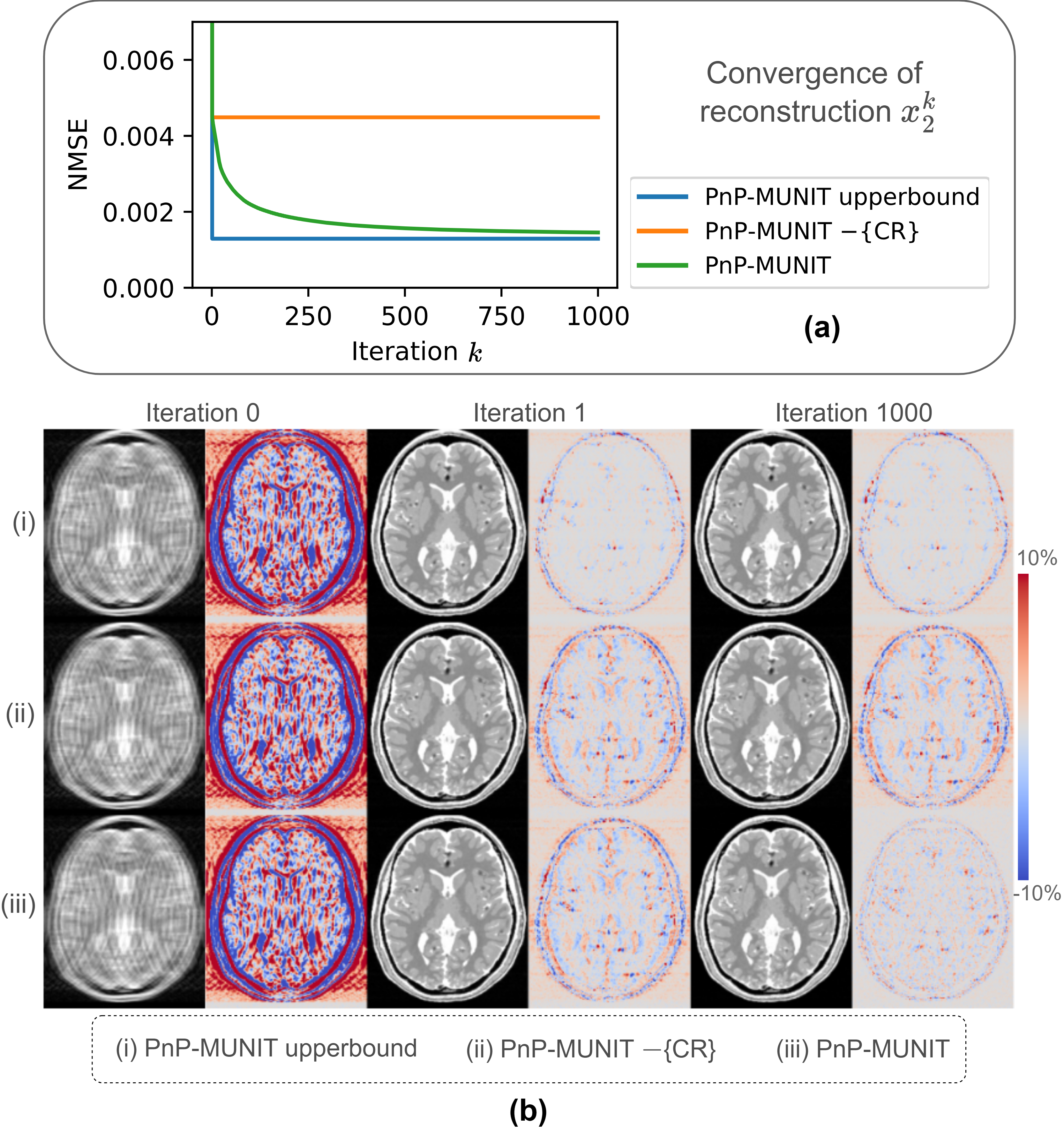
Figure 3: (a) Convergence of PnP-MUNIT and the baseline versions at $R$=4. (b) Evolution of the reconstruction shown with its error map.

We explore here the convergence of PnP-MUNIT by comparing it with two variants. The first uses the content $c_{2}^{*}$ of the ground truth T2W image, thus assuming zero content discrepancy and representing an upper-bound of PnP-MUNIT. The second uses the reference content $c_{1}^{\mathrm{ref}}$ but with CR step disabled, representing a lower-bound of PnP-MUNIT where the non-zero content discrepancy is not corrected. Here as well as in the following simulation experiment, we used the RefSize-1 dataset and the MUNIT-1 model additionally fine-tuned on 2 training volumes for 50k iterations. Fig. 3 shows the convergence curves and intermediate reconstructions. The upper-bound version, given $c_{2}^{*}$, converged in a single iteration, while with $c_{1}^{\mathrm{ref}}$, the ablated version converged equally fast but to a sub-optimal solution. Enabling the CR step closed the gap with the upper-bound, although costing convergence rate.

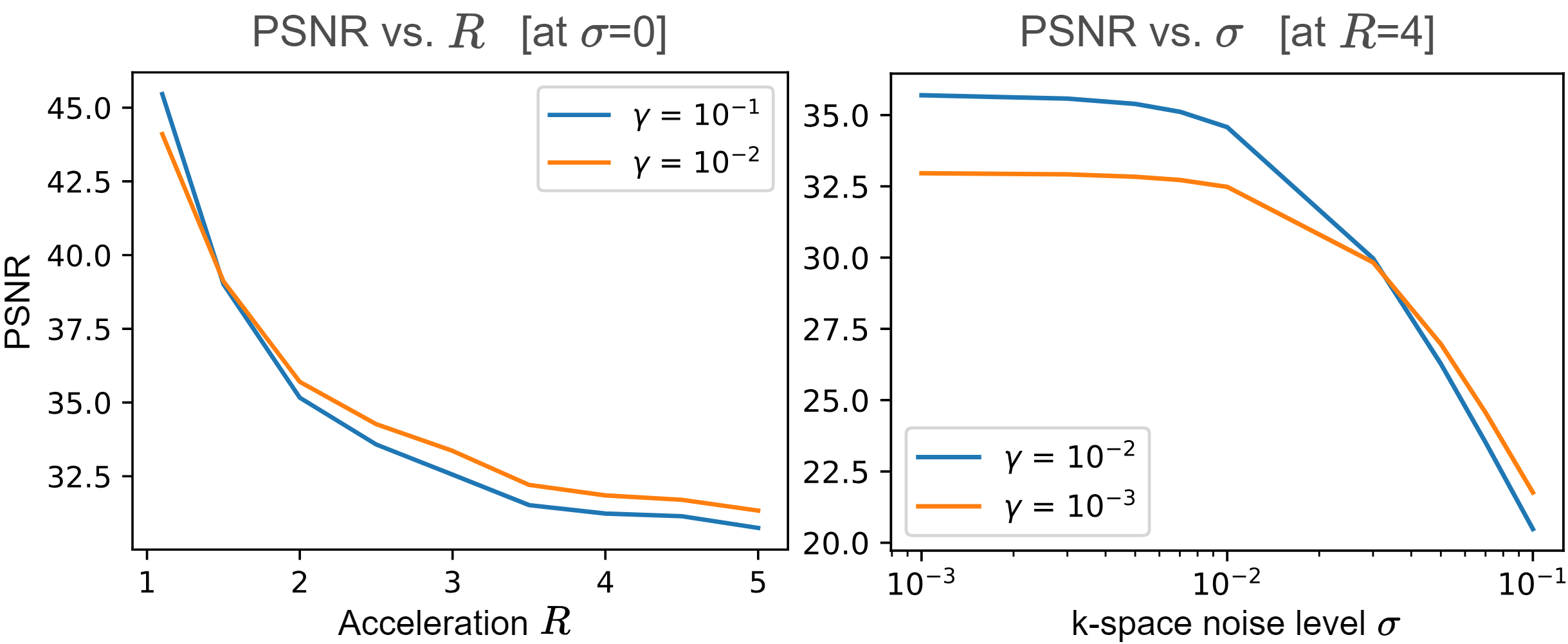
Figure 4: Reconstruction PSNR as a function of acceleration $R$ and k-space noise level $\sigma$ for different values of the $\gamma$ parameter. $\gamma$ controls the consistency of the content with the measured k-space.

IV-A3 Tuning the CR step size

The hyperparameter $\gamma$ in Algorithm 1 controls the CR strength. Fig. 4 shows reconstruction quality as a function of acceleration and k-space noise level, where we observe that the optimal $\gamma$ decreases with the amount and quality of k-space data. This makes sense as enforcing agreement with the k-space gradually becomes less beneficial, thereby contributing less to reconstruction quality.

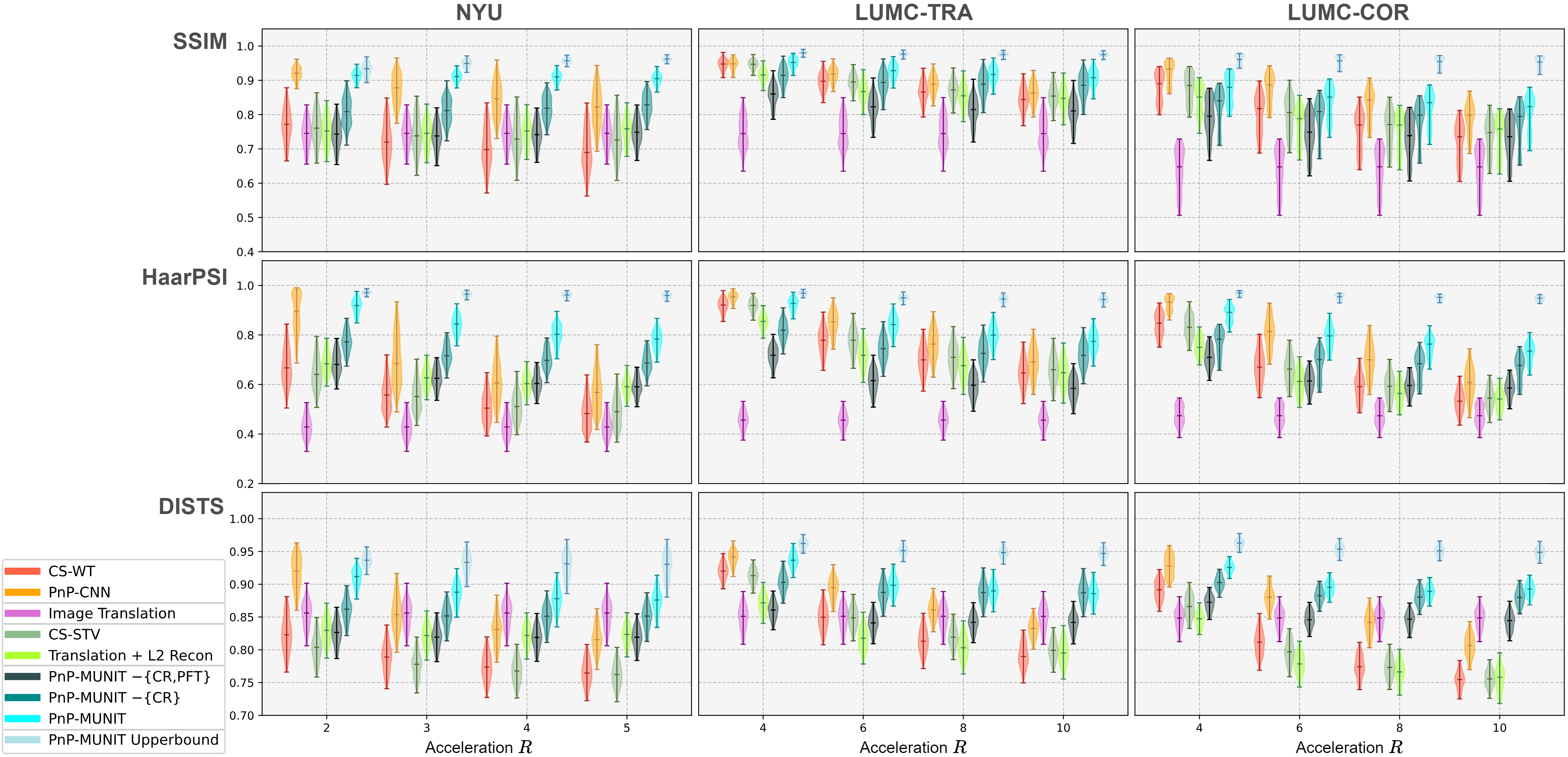
Figure 5: Evaluation plots over recon-test subset of NYU, LUMC-TRA, and LUMC-COR datasets, consisting of 550, 1366, and 200 slices, respectively.

IV-B Benchmark and Ablation

For benchmarking, we used L1-wavelet CS (CS-WT) and PnP-CNN [20] as our single-contrast baselines. The denoising model of PnP-CNN was defined as a 5-layer network with convolution and ReLU operations and a residual connection after the final layer. We additionally compared against deterministic image translation based on MUNIT defined as $x_{2}^{\mathrm{syn}}:=\mathbb{E}_{s_{2}\sim q(s_{2})}[G_{2}(E_{1}^{c}(x^{\mathrm{ref}}_{1}),s_{2})]$. As guided reconstruction baselines, we used STV-based CS (CS-STV) [6] and image translation combined with L2-regularized reconstruction (Translation + L2 recon) [32] given as $\displaystyle\mathop{\min}_{x_{2}}||Ax_{2}-y||_{2}^{2}+\lambda||x_{2}-x_{2}^{\mathrm{syn}}||_{2}^{2}$. For PnP-MUNIT, we ablated PFT and CR to assess their contribution, and finally, as an upper-bound representing zero content discrepancy, we disabled PFT and CR and used the ideal content $c_{2}^{*}$.

TABLE II: Data split for benchmarking. Splits were performed at subject-level, each subject belonging to exactly one subset.

Dataset	Split	Subjects	Sessions	Scans (T1W / T2W)
NYU	model-train	200	200	200 / 200
	model-val	27	27	27 / 27
	recon-val	50	50	50 / 50
	recon-test	50	50	50 / 50
	Total	327	327	327 / 327
LUMC-TRA	model-train	295	418	360 / 415
	model-val	16	17	17 / 17
	recon-val	18	21	21 / 21
	recon-test	20	31	31 / 31
	Total	339	487	429 / 484
LUMC-COR	model-train	242	277	269 / 272
	model-val	18	18	18 / 18
	recon-val	15	18	18 / 18
	recon-test	16	17	17 / 17
	Total	291	330	322 / 325

The NYU brain dataset includes raw data and DICOM scans of 4 contrasts – T1W with and without gadolinium agent, T2W, and FLAIR. Following [33], a DICOM subset of 327 subjects was obtained based on T2W and non-gadolinium T1W scans. Single-coil T2W k-space data was simulated via Fourier transform with 1D Cartesian random sampling of $R\in\{2,3,4,5\}$ and added Gaussian noise of $\sigma=0.01\mathrm{max}(x_{2}^{*})$.

Our in-house datasets consisted of brain scans of patients from LUMC, the use of which was approved for research purpose by the institutional review board. A total of 1669 brain scans were obtained from 817 clinical MR examinations of 630 patients acquired on 3T Philips Ingenia scanners. We focused on accelerating two T2W sequences – (a) 2D T2W TSE transversal (FA=90°, TR=4000-5000ms, TE=80-100ms, ETL=14-18, median voxel size=0.37$\times$0.5mm², median FOV=238$\times$190mm², median slice thickness=3mm, median slices=50), and (b) 2D T2W TSE coronal (FA=90°, TR=2000-3500ms, TE=90-100ms, ETL=17-19, median voxel size=0.39$\times$0.47mm², median FOV=130$\times$197mm², median slice thickness=2mm, median slices=15). For guidance, two corresponding T1W sequences were used – (a) 3D T1W TFE transversal (FA=8°, TR=9.8-9.9ms, TE=4.6ms, ETL=200, median voxel size=0.98$\times$0.99$\times$0.91mm³, median FOV=238$\times$191$\times$218mm³), and (b) 3D T1W TSE coronal (FA=80-90°, TR=500-800ms, TE=6.5-16ms, ETL=10-13, median voxel size=0.59$\times$0.62$\times$1.19mm³, median FOV=130$\times$238$\times$38mm³). The transversal and coronal protocols were considered as two separate datasets, namely LUMC-TRA and LUMC-COR. The multi-coil T2W raw data comprised of 6-channel (LUMC-TRA) and 13-channel (LUMC-COR) k-space and coil sensitivity maps. This k-space was already undersampled (1D Cartesian random) at acquisition with clinical acceleration of $R$=1.8-2. We further undersampled it retrospectively to higher accelerations $R\in\{4,6,8,10\}$ by dropping subsets of the acquired lines.

Each dataset was split into 4 subsets – (a) model-train, (b) model-val, (c) recon-val, and (d) recon-test. The former two were used to train and tune the plug-and-play models, recon-val to tune the reconstruction algorithms, and recon-test as the held-out test set. An overview of the data split is shown in Table II. Additionally, 20 subjects from model-train were designated for PFT. Spatially aligned images required by all except the unpaired training set were obtained via rigid registration using Elastix [38]. We empirically found the ContentSize-1 and ContentSize-2 configurations as optimal for the NYU and LUMC datasets, respectively, which reflects the lower effective content and hence greater difficulty of the LUMC datasets. For each dataset, the model was pre-trained and fine-tuned for 400k and 50k iterations, respectively. We used 3 perceptual metrics for evaluation: SSIM, HaarPSI, and DISTS. While SSIM is commonly used, HaarPSI and DISTS are known to correlate better with visual judgment of image quality [39]. All three metrics are bounded to $[0,1]$ with $1$ representing perfect image quality. We additionally conducted paired Wilcoxon signed-rank tests to measure statistical significance when comparing pairs of algorithms.

Fig. 5 plots the benchmark metrics, which can be summarized in the following three trends. First, pure image translation was worse compared to single-contrast reconstruction, especially at lower acceleration factors (comparing with PnP-CNN, $p$$<$0.05 for all metrics and datasets). Combining it with L2-regularized reconstruction improved SSIM and HaarPSI ($p$$<$0.05 for all datasets and accelerations except SSIM at $R$=3 in NYU), but not necessarily DISTS, suggesting that the the available complementary information was not fully utilized. PnP-MUNIT was consistently better than both image translation and naive guidance ($p$$<$0.05 throughout for both cases). It also outperformed the conventional guided CS-STV ($p$$<$0.05 throughout, except SSIM at $R$=4 in LUMC-COR). Second, both PnP-CNN and PnP-MUNIT performed similarly at lower acceleration. At higher acceleration, PnP-MUNIT outperformed PnP-CNN ($p$$<$0.05 for all metrics and datasets except SSIM at $R$=8 in LUMC-COR). Third, introducing PFT and CR into the ablated PnP-MUNIT improved the reconstructions ($p$$<$0.05 throughout in both cases except in DISTS for the latter at $R$=10 in LUMC-TRA). The contribution of PFT was almost constant across $R$, whereas that of CR decreased with $R$, which was expected since CR depends on the measured k-space data to refine the content.

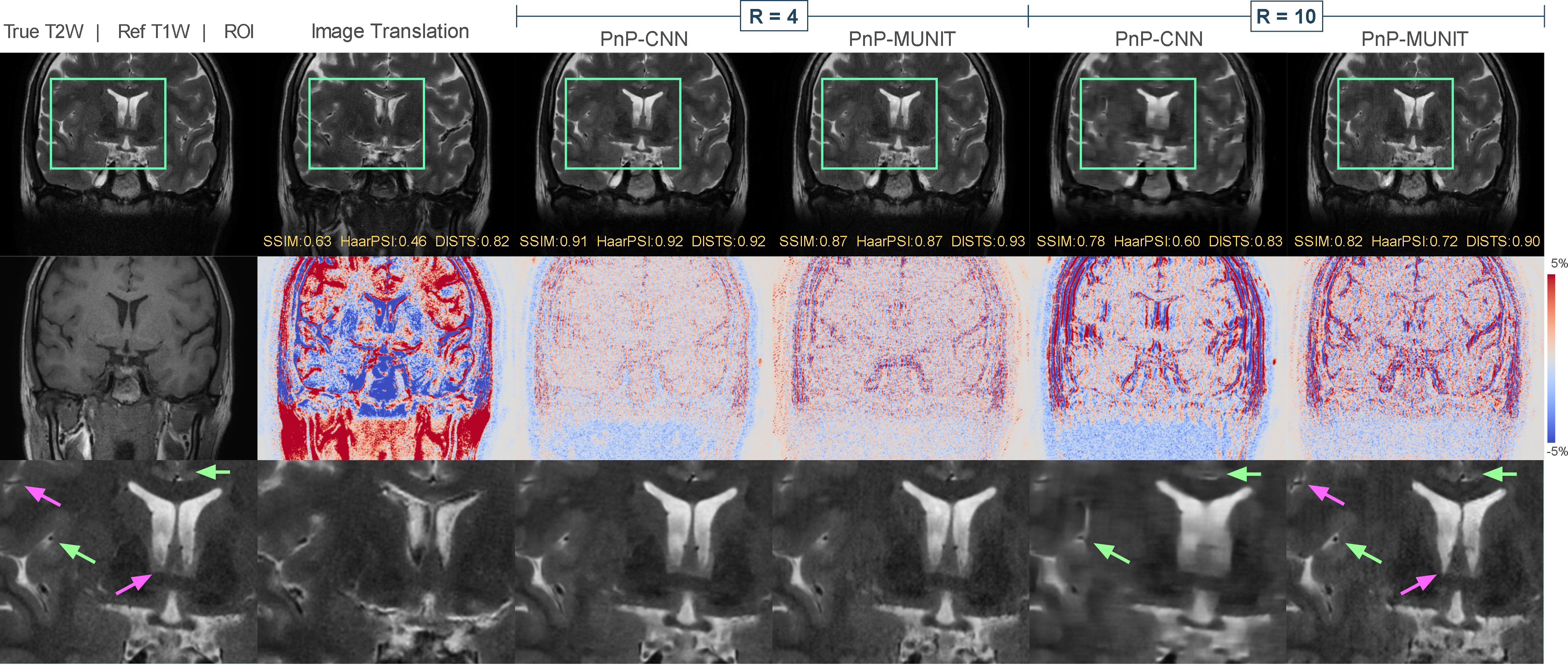
Figure 6: Sample slice from the LUMC-COR recon-test set comparing PnP-MUNIT with PnP-CNN and pure image translation.

Fig. 6 shows an example from LUMC-COR representative of the first two trends. Image translation produced severe anatomical defects and predicted structure in the lower region of the image where the ground truth contains low signal. At $R$=4, PnP-MUNIT was visually similar to PnP-CNN, with the main difference being a blur effect in PnP-CNN and mild texture artifacts in PnP-MUNIT. At $R$=10, PnP-CNN reconstruction was non-viable, containing severe blur and artifacts (green arrows). On the other hand, PnP-MUNIT did not degrade much from the $R$=4 case and most fine structures were sharply resolved (green arrows). However, an interesting failure mode of PnP-MUNIT at high acceleration was the subtle localized distortions in the anatomy (pink arrows).

IV-C Radiological Evaluation

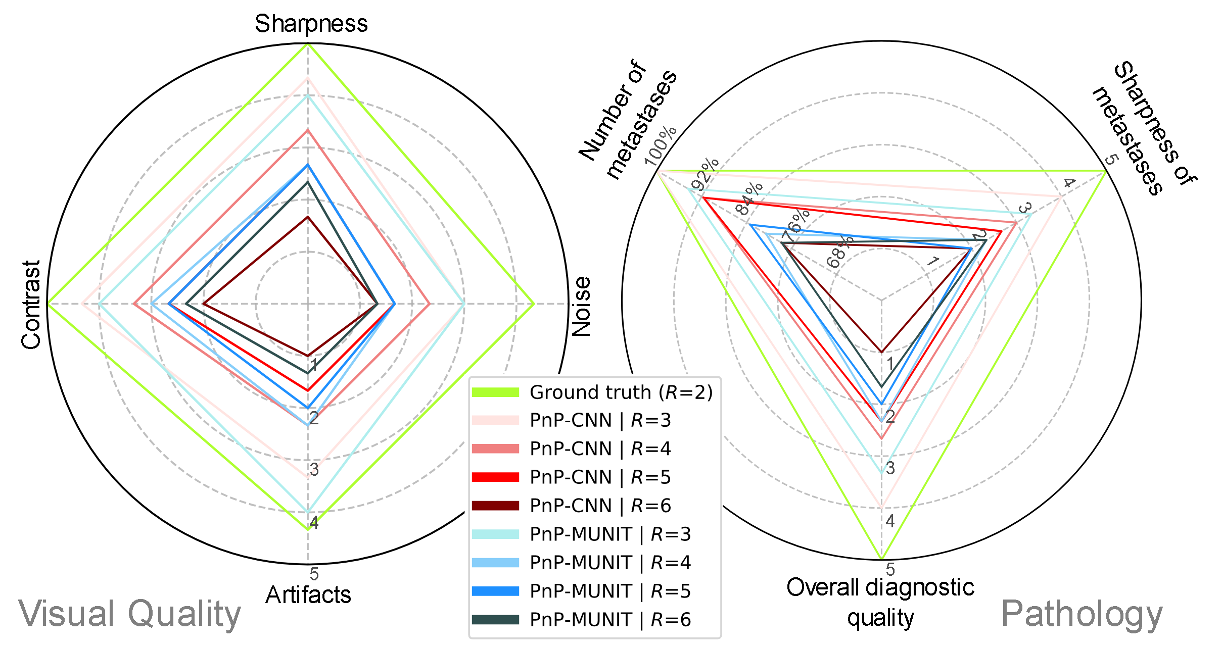
Figure 7: Averaged results of the radiological evaluation.

We conducted the radiological evaluation on a small sample of LUMC-TRA recon-test set. We selected 3 cases that showed brain metastases in corresponding gadolinium-enhanced T1W scans. The evaluation comprised two parts, namely visual quality and pathology. Four visual quality criteria were used, namely sharpness, noise, artifacts, and contrast between gray and white matter and CSF. For pathology, we used three criteria, namely the number and sharpness of hyperintense areas within or surrounding metastases and the overall diagnostic quality of the scan for brain metastases. The images were scored using a five-point Likert scale [40] – (1) non-diagnostic, (2) poor, (3) fair, (4) good, and (5) excellent diagnostic quality. We considered PnP-MUNIT and PnP-CNN at 4 clinically realistic accelerations $R\in\{3,4,5,6\}$. In total, 9 images per patient, including the reconstructions and the clinical ground truth of $R$=2, were presented to a senior neuroradiologist who scored each image individually, blinded to the reconstruction method and $R$. Figure 7 plots the evaluation result. At $R$=3, both algorithms produced at least “fairly diagnostic” reconstructions and allowed the detection of more than 90% of metastases. PnP-CNN was better than PnP-MUNIT at $R\in\{3,4\}$ in terms of sharpness, contrast, and the pathology criteria. At $R$=5, PnP-MUNIT matched or exceeded PnP-CNN in terms of visual quality, although being worse in terms of pathology criteria. At $R$=6, PnP-CNN sharply dropped to non-diagnostic level, whereas PnP-MUNIT was better, especially in terms of sharpness and contrast as well as in overall diagnostic quality.

V Discussion

We explored the interpretability aspect of PnP-MUNIT in terms of the effective content in a two-contrast dataset (Section IV-A1) and obtained a notion of limit to guided reconstruction in terms of the reference image resolution. This limit would indeed depend on more fundamental factors such as MR sequence types, which we did not investigate here. Our data-driven definition of content and style is loosely analogous to MR physics-based descriptions of quantitative tissue maps and acquisition-related factors. Hence, a further level of interpretability could be achieved by constraining the learned content to represent physically meaningful tissue parameters. Content discrepancy is characterized as a limiting factor in guided reconstruction (Section III-C) and plays a major role throughout this work. Viewed as a set of quasi tissue maps, estimating content from a single image is challenging, ideally requiring a time series of images, which captures the magnetization dynamics. Content discrepancy is, therefore, inevitable. We proposed two complementary ways to minimize its effect on the reconstruction. While paired fine-tuning improves the model using a small amount of paired data, content refinement (CR) corrects for the remaining discrepancy adaptively during reconstruction using the measured k-space. A drawback of CR, however, is slower convergence (Section IV-A2). This could be mitigated by partially adopting an unrolled network design. The resulting tradeoff between model latency and generalizability would be interesting to explore.

Unpaired pre-training of the content/style model boosts the practical applicability of PnP-MUNIT, e.g. in the case of LUMC-TRA where the T1W/T2W data imbalance is considerable. In this work, we limited our baselines to those algorithms that closely resemble ours in terms of design or data requirement. As future work, a more comprehensive study could be conducted with a broader range of methods and evaluation criteria, e.g. comparing generalizability across accelerations and sampling patterns with guided unrolled networks, given a fixed budget of paired training data. At reconstruction time, we assumed the reference and reconstruction images to be spatially aligned. The CR update, which can correct minor registration errors implicitly, would likely break down at the typically observed levels of patient motion. A potential solution is to incorporate an online registration step to explicitly and efficiently correct for arbitrary inter-scan motion, thereby further relaxing the overall data constraints.

In terms of reconstruction quality, we observed (Section IV-B) that using both measured k-space and reference scan via PnP-MUNIT was more beneficial than (a) using either one of them and (b) combining both in a naive way or based on hand-crafted prior, suggesting that our approach maximally exploits the complementary information. Compared to PnP-CNN, PnP-MUNIT allowed up to 32.6% more acceleration for a given SSIM. In the radiological task (Section IV-C), PnP-MUNIT produced diagnostic-quality reconstructions at $R$=3, a difference of 33.3% over the clinical reconstructions of $R$=2. However, it was somewhat worse than PnP-CNN, while theoretically, the additional guidance should result in at least equivalent image quality. We argue that the likely cause is the limitations of the dataset and the specific content/style model, not of the proposed general approach. First, in LUMC-TRA, T1W scans had 2-3 times lower resolution than T2W scans, limiting the value of guidance (Section IV-A1). In the long run, this may be solved by co-designing a higher-resolution reference sequence with the target sequence to optimize guidance. Second, and more importantly, correcting for content discrepancy using CR relies on computing gradients through the decoder $G_{2}$. If $G_{2}$ is highly non-linear and the reference content is not sufficiently close to the optimum, CR may converge to a sub-optimal point leading to texture artifacts in the reconstruction, as seen in Fig. 6 at $R$=4. In the radiological study, precisely this phenomenon is likely to have impacted the visual and diagnostic quality of PnP-MUNIT. Hence, to improve clinical utility, the content/style model must be improved using specialized architecture and regularization.

VI Conclusion

In this work, we introduced PnP-MUNIT, a novel approach to multi-contrast reconstruction combining content/style modeling with iterative reconstruction, which is interpretable in that it allows the two stages to be analyzed separately. By exploring the interpretability aspect, two limiting factors of guided reconstruction were identified – the amount of effective content in a two-contrast dataset and content discrepancy. On real-world clinical data, PnP-MUNIT provided up to 32.6% more acceleration over PnP-CNN for a given SSIM, enabling sharper reconstructions at high accelerations. Given the radiological task of visual quality assessment and brain metastasis diagnosis at realistic accelerations, PnP-MUNIT produced diagnostic-quality images at $R$=3, enabling 33.3% more acceleration over clinical reconstructions. To progress towards a practical implementation, future work will focus on improving the content/style model and reconstruction latency and incorporating online registration into the reconstruction.

References

- [1] K. P. Pruessmann, M. Weiger, P. Börnert, and P. Boesiger, “Advances in sensitivity encoding with arbitrary k-space trajectories,” Magnetic Resonance in Medicine, vol. 46, no. 4, pp. 638–651, 2001.
- [2] M. A. Griswold, P. M. Jakob, R. M. Heidemann, M. Nittka, V. Jellus, J. Wang, B. Kiefer, and A. Haase, “Generalized Autocalibrating Partially Parallel Acquisitions (GRAPPA),” Magnetic Resonance in Medicine, vol. 47, no. 6, pp. 1202–1210, 2002.
- [3] M. Lustig, D. Donoho, and J. M. Pauly, “Sparse MRI: The Application of Compressed Sensing for Rapid MR Imaging,” Magnetic Resonance in Medicine, vol. 58, no. 6, pp. 1182–1195, 2007.
- [4] N. Pezzotti, S. Yousefi, M. S. Elmahdy, J. H. F. Van Gemert, C. Schuelke, M. Doneva, T. Nielsen, S. Kastryulin, B. P. F. Lelieveldt, M. J. P. Van Osch, E. De Weerdt, and M. Staring, “An Adaptive Intelligence Algorithm for Undersampled Knee MRI Reconstruction,” IEEE Access, vol. 8, pp. 204825–204838, 2020.
- [5] P. Seow, S. W. Kheok, M. A. Png, P. H. Chai, T. S. T. Yan, E. J. Tan, L. Liauw, Y. M. Law, C. V. Anand, W. Lee, et al., “Evaluation of Compressed SENSE on Image Quality and Reduction of MRI Acquisition Time: A Clinical Validation Study,” Academic Radiology, vol. 31, no. 3, pp. 956–965, 2024.
- [6] M. J. Ehrhardt and M. M. Betcke, “Multicontrast MRI Reconstruction with Structure-Guided Total Variation,” SIAM Journal on Imaging Sciences, vol. 9, pp. 1084–1106, Jan. 2016.
- [7] L. Weizman, Y. C. Eldar, and D. Ben Bashat, “Reference-based MRI,” Medical Physics, vol. 43, no. 10, pp. 5357–5369, 2016.
- [8] B. Zhou and S. K. Zhou, “DuDoRNet: Learning a Dual-domain Recurrent Network for Fast MRI Reconstruction with Deep T1 Prior,” in Proceedings of the IEEE/CVF Conference on Computer Vision and Pattern Recognition, pp. 4273–4282, 2020.
- [9] B. Bilgic, V. K. Goyal, and E. Adalsteinsson, “Multi-contrast Reconstruction with Bayesian Compressed Sensing,” Magnetic Resonance in Medicine, vol. 66, no. 6, pp. 1601–1615, 2011.
- [10] J. Huang, C. Chen, and L. Axel, “Fast Multi-contrast MRI Reconstruction,” Magnetic Resonance Imaging, vol. 32, no. 10, pp. 1344–1352, 2014.
- [11] E. Kopanoglu, A. Güngör, T. Kilic, E. U. Saritas, K. K. Oguz, T. Çukur, and H. E. Güven, “Simultaneous Use of Individual and Joint Regularization Terms in Compressive Sensing: Joint Reconstruction of Multi-channel Multi-contrast MRI Acquisitions,” NMR in Biomedicine, vol. 33, no. 4, p. e4247, 2020.
- [12] Y. Yang, N. Wang, H. Yang, J. Sun, and Z. Xu, “Model-driven Deep Attention Network for Ultra-fast Compressive Sensing mri Guided by Cross-contrast MR Image,” in Medical Image Computing and Computer Assisted Intervention (MICCAI), pp. 188–198, Springer, 2020.
- [13] K. Pooja, Z. Ramzi, G. Chaithya, and P. Ciuciu, “Mc-pdnet: Deep Unrolled Neural Network for Multi-contrast MR Image Reconstruction from Undersampled k-space Data,” in IEEE International Symposium on Biomedical Imaging (ISBI), pp. 1–5, IEEE, 2022.
- [14] B. Levac, A. Jalal, K. Ramchandran, and J. I. Tamir, “Mri reconstruction with side information using diffusion models,” in 2023 57th Asilomar Conference on Signals, Systems, and Computers, pp. 1436–1442, IEEE, 2023.
- [15] S. U. Dar, M. Yurt, L. Karacan, A. Erdem, E. Erdem, and T. Çukur, “Image Synthesis in Multi-Contrast MRI With Conditional Generative Adversarial Networks,” IEEE Transactions on Medical Imaging, vol. 38, pp. 2375–2388, Oct. 2019.
- [16] M. Yurt, S. U. Dar, A. Erdem, E. Erdem, K. K. Oguz, and T. Çukur, “mustGAN: Multi-stream Generative Adversarial Networks for MR Image Synthesis,” Medical Image Analysis, vol. 70, p. 101944, May 2021.
- [17] J. Denck, J. Guehring, A. Maier, and E. Rothgang, “MR-contrast-aware Image-to-Image Translations with Generative Adversarial Networks,” International Journal of Computer Assisted Radiology and Surgery, vol. 16, Dec. 2021.
- [18] M.-Y. Liu, T. Breuel, and J. Kautz, “Unsupervised Image-to-image Translation Networks,” Advances in Neural Information Processing Systems, vol. 30, 2017.
- [19] X. Huang, M.-Y. Liu, S. Belongie, and J. Kautz, “Multimodal Unsupervised Image-to-Image Translation,” in Proceedings of the European Conference on Computer Vision (ECCV), pp. 172–189, 2018.
- [20] R. Ahmad, C. A. Bouman, G. T. Buzzard, S. Chan, S. Liu, E. T. Reehorst, and P. Schniter, “Plug-and-play Methods for Magnetic Resonance Imaging using Denoisers for Image Recovery,” IEEE Signal Processing Magazine, vol. 37, no. 1, pp. 105–116, 2020.
- [21] U. S. Kamilov, C. A. Bouman, G. T. Buzzard, and B. Wohlberg, “Plug-and-play Methods for Integrating Physical and Learned Models in Computational Imaging: Theory, Algorithms, and Applications,” IEEE Signal Processing Magazine, vol. 40, no. 1, pp. 85–97, 2023. Publisher: IEEE.
- [22] C. Rao, L. Beljaards, M. van Osch, M. Doneva, J. Meineke, C. Schuelke, N. Pezzotti, E. de Weerdt, and M. Staring, “Guided Multicontrast Reconstruction based on the Decomposition of Content and Style,” in International Society for Magnetic Resonance in Medicine (ISMRM), 2024.
- [23] A. Chambolle, R. A. De Vore, N.-Y. Lee, and B. J. Lucier, “Nonlinear Wavelet Image Processing: Variational Problems, Compression, and Noise Removal through Wavelet Shrinkage,” IEEE Transactions on Image Processing, vol. 7, no. 3, pp. 319–335, 1998.
- [24] S. Boyd, N. Parikh, E. Chu, B. Peleato, J. Eckstein, et al., “Distributed optimization and statistical learning via the alternating direction method of multipliers,” Foundations and Trends® in Machine learning, vol. 3, no. 1, pp. 1–122, 2011.
- [25] J. Schlemper, J. Caballero, J. V. Hajnal, A. N. Price, and D. Rueckert, “A Deep Cascade of Convolutional Neural Networks for Dynamic MR Image Reconstruction,” IEEE Transactions on Medical Imaging, vol. 37, no. 2, pp. 491–503, 2017.
- [26] H. K. Aggarwal, M. P. Mani, and M. Jacob, “MoDL: Model-based Deep Learning Architecture for Inverse Problems,” IEEE Transactions on Medical Imaging, vol. 38, no. 2, pp. 394–405, 2018.
- [27] X. Liu, J. Wang, S. Lin, S. Crozier, and F. Liu, “Optimizing Multicontrast MRI Reconstruction with Shareable Feature Aggregation and Selection,” NMR in Biomedicine, vol. 34, no. 8, p. e4540, 2021.
- [28] X. Liu, J. Wang, H. Sun, S. S. Chandra, S. Crozier, and F. Liu, “On the Regularization of Feature Fusion and Mapping for Fast MR Multi-contrast Imaging via Iterative Networks,” Magnetic Resonance Imaging, vol. 77, pp. 159–168, 2021.
- [29] P. Isola, J.-Y. Zhu, T. Zhou, and A. A. Efros, “Image-to-image Translation with Conditional Adversarial Networks,” in Proceedings of the IEEE Conference on Computer Vision and Pattern Recognition, pp. 1125–1134, 2017.
- [30] J.-Y. Zhu, T. Park, P. Isola, and A. A. Efros, “Unpaired Image-to-image Translation using Cycle-consistent Adversarial Networks,” in Proceedings of the IEEE International Conference on Computer Vision, pp. 2223–2232, 2017.
- [31] G. Oh, B. Sim, H. Chung, L. Sunwoo, and J. C. Ye, “Unpaired Deep Learning for Accelerated MRI using Optimal Transport Driven CycleGAN,” IEEE Transactions on Computational Imaging, vol. 6, pp. 1285–1296, 2020.
- [32] S. U. Dar, M. Yurt, M. Shahdloo, M. E. Ildız, B. Tınaz, and T. Çukur, “Prior-Guided Image Reconstruction for Accelerated Multi-Contrast MRI via Generative Adversarial Networks,” IEEE Journal of Selected Topics in Signal Processing, vol. 14, pp. 1072–1087, Oct. 2020.
- [33] K. Xuan, L. Xiang, X. Huang, L. Zhang, S. Liao, D. Shen, and Q. Wang, “Multimodal MRI Reconstruction Assisted with Spatial Alignment Network,” IEEE Transactions on Medical Imaging, vol. 41, no. 9, pp. 2499–2509, 2022.
- [34] E. Richardson and Y. Weiss, “The Surprising Effectiveness of Linear Unsupervised Image-to-Image Translation,” in 2020 25th International Conference on Pattern Recognition (ICPR), pp. 7855–7861, Jan. 2021.
- [35] D. L. Collins, A. P. Zijdenbos, V. Kollokian, J. G. Sled, N. J. Kabani, C. J. Holmes, and A. C. Evans, “Design and Construction of a Realistic Digital Brain Phantom,” IEEE Transactions on Medical Imaging, vol. 17, no. 3, pp. 463–468, 1998.
- [36] F. Knoll, J. Zbontar, A. Sriram, M. J. Muckley, M. Bruno, A. Defazio, M. Parente, K. J. Geras, J. Katsnelson, H. Chandarana, et al., “fastMRI: A Publicly Available Raw k-space and DICOM Dataset of Knee Images for Accelerated MR Image Reconstruction using Machine Learning,” Radiology: Artificial Intelligence, vol. 2, no. 1, p. e190007, 2020.
- [37] J. Zbontar, F. Knoll, A. Sriram, T. Murrell, Z. Huang, M. Muckley, A. Defazio, R. Stern, P. Johnson, M. Bruno, et al., “fastMRI: An Open Dataset and Benchmarks for Accelerated MRI,” arXiv preprint arXiv:1811.08839, 1811.
- [38] S. Klein, M. Staring, K. Murphy, M. A. Viergever, and J. P. Pluim, “Elastix: A Toolbox for Intensity-based Medical Image Registration,” IEEE Transactions on Medical Imaging, vol. 29, no. 1, pp. 196–205, 2009.
- [39] S. Kastryulin, J. Zakirov, N. Pezzotti, and D. V. Dylov, “Image Quality Assessment for Magnetic Resonance Imaging,” IEEE Access, vol. 11, pp. 14154–14168, 2023. Publisher: IEEE.
- [40] A. Mason, J. Rioux, S. E. Clarke, A. Costa, M. Schmidt, V. Keough, T. Huynh, and S. Beyea, “Comparison of Objective Image Quality Metrics to Expert Radiologists’ Scoring of Diagnostic Quality of MR Images,” IEEE Transactions on Medical Imaging, vol. 39, no. 4, pp. 1064–1072, 2019.