Stimulus-to-stimulus learning in RNNs with cortical inductive biases

Summary

Animals learn to predict external contingencies from experience through a process of conditioning. A natural mechanism for conditioning is stimulus substitution, whereby the neuronal response to a stimulus with no prior behavioral significance becomes increasingly identical to that generated by a behaviorally significant stimulus it reliably predicts. We propose a recurrent neural network model of stimulus substitution which leverages two forms of inductive bias pervasive in the cortex: representational inductive bias in the form of mixed stimulus representations, and architectural inductive bias in the form of two-compartment pyramidal neurons that have been shown to serve as a fundamental unit of cortical associative learning. The properties of these neurons allow for a biologically plausible learning rule that implements stimulus substitution, utilizing only information available locally at the synapses. We show that the model generates a wide array of conditioning phenomena, and can learn large numbers of associations with an amount of training commensurate with animal experiments, without relying on parameter fine-tuning for each individual experimental task. In contrast, we show that commonly used Hebbian rules fail to learn generic stimulus-stimulus associations with mixed selectivity, and require task-specific parameter fine-tuning. Our framework highlights the importance of multi-compartment neuronal processing in the cortex, and showcases how it might confer cortical animals the evolutionary edge.

Keywords. Associative learning, classical conditioning, recurrent neural networks, synaptic plasticity, predictive coding, stimulus substitution, mixed selectivity, compartmentalized neuron, self-supervised learning, surprise.

Introduction

The ability to forecast important events is necessary for effective behavior. Animals are equipped with innate reflexes to tackle common threats and to exploit opportunities in their environment. However, given the complex and changing nature of the world, animals also need to acquire new reflexes by learning from experience. This process involves the association or conditioning of an initially neutral stimulus (conditioned stimulus, CS) with another stimulus intrinsically related to primary reward or punishment (unconditioned stimulus, US). If learning is successful, the CS can then induce the same behavioral response as the US. Initially proposed by Pavlov, this type of learning is known as classical conditioning.

A potential mechanism for conditioning is stimulus substitution [1]. Under this mechanism, the response of the relevant population of neurons to the CS becomes increasingly identical to that generated by the US. After this, any downstream processes that are normally triggered by the US are also triggered by the CS. Behavioral evidence in favor of stimulus substitution comes from studies showing that animals display the same behavior to the CS as to the US, even when the behavior is not appropriate (e.g. consummatory response towards a light that has been associated with food), and that the behavior is reinforcer dependent [1]. Furthermore, recent experiments show that during conditioning the response of S1 pyramidal neurons to the CS becomes increasingly similar to their response to the US, a phenomenon the authors termed “learning induced neuronal identity switch”, and that this change correlates with learning performance [2].

A basic goal in computational and cognitive neuroscience is to build plausible models of neural network architectures capable of accounting for psychological phenomena. Previous work has shown that three-factor Hebbian synaptic plasticity rules accounts for a wide gamut of conditioning phenomena [3, 4, 5, 6]. However, these models have some important limitations. First, they fail to capture the generality of pattern-to-pattern associations implicit in stimulus substitution, where both the US and the CS correspond to population activity patterns. Some use learning rules requiring storage of recent events at each synapse [5], while most assume that the tuning of neurons to stimuli is demixed, allowing simple reward modulated spike-timing-dependent plasiticy to establish the appropriate mappings [5, 6]. These assumptions are inconsistent with the well-established fact that representations throughout the brain are high-dimensional and mixed [7].

In this study we propose a recurrent neural network (RNN) model of stimulus substitution. Critically, the model learns pattern-to-pattern associations using only biologically plausible local plasticity, and individual neurons are tuned to multiple behavioral stimuli, which gives rise to mixed representations of the CSs and USs. While subcortical [8] and even single-neuron [9] mechanisms for conditioning exist, our model is focused on stimulus-stimulus learning in the cortex, where the use of mixed stimulus representation allows learning a wide and flexible range of associations within the same neuronal network, which confers an evolutionary edge.

To achieve this goal, we leverage two forms of biological inductive bias built into the cortex: first, representational inductive bias in the form of mixed stimulus representations, that permit the efficient packing of multiple associations within the same neuronal population. To combat the additional complexity introduced by mixed representations, which requires not just the activation of the correct neurons but also the correct activity level, we leverage the second form of inductive bias: architectural inductive bias in the form of two-compartment layer-5 pyramidal neurons which are prevalent in the cortex [10].

We propose a RNN model of such two-compartment neurons. Recent work has shown that these neurons can learn to be predictive of a reward [11], and suggests that they could serve as a fundamental unit of associative learning in the cortex through a built-in cellular mechanism [12]. Hence, we refer to them as associative neurons. The term associative here does not have a strictly Hebbian interpretation; rather it refers to the hetero-associative capacity of these neurons to link together information originating from different streams [13], through a mechanism known as BAC firing [14]. The properties of these neurons allow for a biologically plausible learning rule that utilizes only information available locally at the synapses, and that is capable of inducing self-supervised predictive plasticity [15, 16], which allows neurons to respond with the same firing rate to the CS as they would to the US, i.e. achieve stimulus substitution.

We show that the model generates a wide array of conditioning phenomena, including delay conditioning, trace conditioning, extinction, blocking, overshadowing, saliency effects, overexpectation, contingency effects and faster reacquisition of previous learnt associations. Furthermore, it can learn large numbers of CS-US associations with an amount of training commensurate with animal experiments, without relying on parameter fine-tuning for each individual experimental task. In contrast, we show that Hebbian learning rules, including three-factor extensions of Oja’s rule [17] and the BCM rule [18], fail to learn generic stimulus-to-stimulus associations due to their unsupervised nature, and require task specific parameter fine-tuning.

Results

Model setup

In classical conditioning animals learn to predict the upcoming appearance of an unconditioned stimulus (US, e.g. food) after the presentation of a conditioned stimulus (CS, e.g. bell ring). As shown in fig. 1A, trials start with the presentation of the CS, which lasts until $t_{\text{cs-off}}$. The US is presented at $t_{\text{us-on}}$, and lasts until the end of the trial. Each trial has a fixed duration of $t_{\text{trial}}$ seconds. If the US appears before the CS disappears, the task involves delay conditioning. In contrast, if the CS disappears before the US is shown, the task involves trace conditioning, with $t_{\text{delay}}=t_{\text{us-on}}-t_{\text{cs-off}}$ denoting the delay between the two stimuli. In our task animals need to learn $N_{\text{stim}}$ different CS-US pairs. Every trial one pair is randomly chosen, and the corresponding CS is shown followed by its associated US.

We model a RNN of associative neurons (fig. 1C, yellow background) that represents the stimuli using mixed population representations and is capable of learning all of the CS-US associations using only local information available at the synapses. The inputs to the model are time-dependent vectors $r_{\text{cs}}(t)$ and $r_{\text{us}}(t)$, of dimension $N_{\text{inp}}$, that encode the presence and identity of the CS and the US. For simplicity, these vectors are represented by unique Boolean vectors, and they take the value of the stimulus while it is shown, and zero otherwise. The vectors are randomly generated, subject to a constraint for a minimal Hamming distance $H_{\text{d}}$ between any two vectors of the same type. This minimal separation limits the extent to which learning on any give pair impairs learning of the other associations. The output of the associative network is an estimate of the US vector $r_{\text{us}}$, denoted $\hat{r}_{\text{us}}$, which is decoded from network activity at all times (see fig. 1C and “US decoding” in Methods).

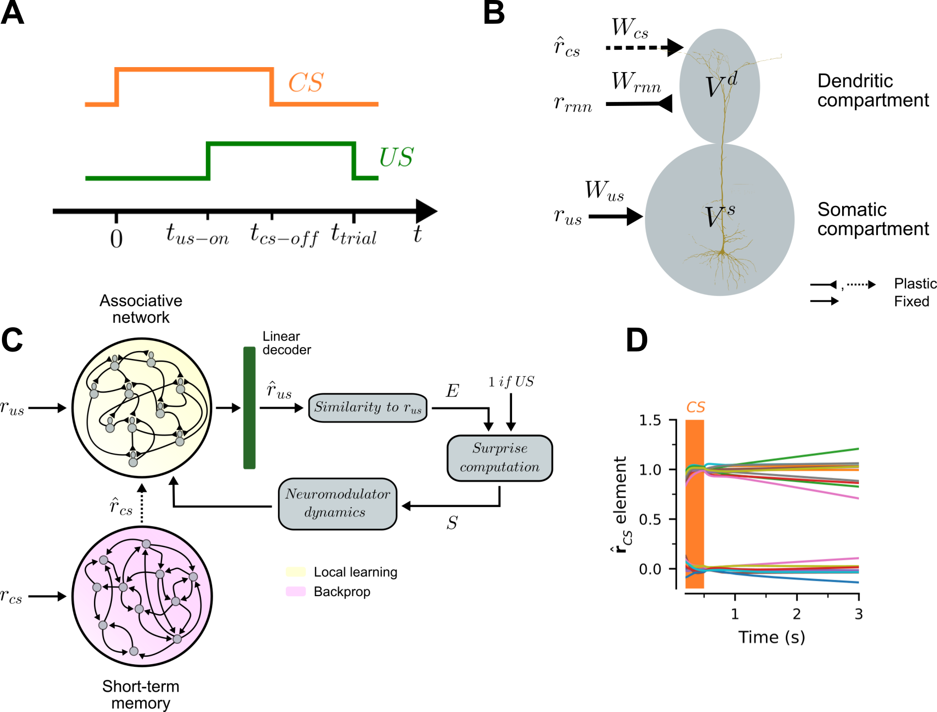
Figure 1: Model. (A) Every trial has a duration of $t_{\text{trial}}$ seconds. Trials start with the presentation of a CS, which disappears after time $t_{\text{cs-off}}$. The associated US appears at time $t_{\text{us-on}}$ and stays until the end of the trial. The network has to learn $N_{\text{stim}}$ unique CS-US pairs. (B) Associative neurons are modeled as an abstraction of a layer-5 cortical pyramidal neuron. $V^{\text{s}}$ and $V^{\text{d}}$ denote the voltage in the somatic and dendritic compartments. The somatic compartment receives as input a Boolean vector $r_{\text{us}}$ representing the US. The dendritic compartment receives as inputs a vector $\hat{r}_{\text{cs}}$ with a short-term memory representation of the CS, as well as recursive activity from all other neurons in the RNN. The matrices $W_{\text{rnn}}$, $W_{\text{cs}}$ and $W_{\text{us}}$ denote the synaptic weights for the inputs. $W_{\text{us}}$ is fixed throughout the experiment. $W_{\text{rnn}}$ and $W_{\text{cs}}$ are updated over trials with training. (C) Full outline of the model. The associative network is made of $N_{\text{rnn}}$ associative neurons. The US is presented directly to the associative neurons, whereas the CS is presented to a short-term memory circuit that produces the short-term memory representation $\hat{r}_{\text{cs}}$. Learning in the associated network is gated by a surprise signal which measures the extent to which the US, or its absence, was anticipated. The surprise signal is computed in three steps. First, throughout the trial a linear decoder is used to obtain an estimate $\hat{r}_{\text{us}}$ of the US from the population vector of the associative network, denoted by $r_{\text{rnn}}$. Second, an expectation $E^{i}$ is formed according for each US based on the similarity between $r^{i}_{\text{us}}$ and $\hat{r}_{\text{us}}$. These expectations determine the level of surprise $S$ associated with the arrival or absence of the US, which then gives rise to neuromodulator dynamics that gate learning in the associative network. (D) Performance of the short-term memory network in a single trial when CSs are presented only for 500 ms. We plot the output of the memory network for several seconds. Each color denotes a different element in $r_{\text{cs}}$.

The fundamental unit of computation in the associative network is the associative neuron, a two-compartment neuron modelled after layer-5 pyramidal cells in the cortex (fig. 1B). A crucial property of the associative neuron is that it can separate incoming “feedforward” inputs from “feedback” ones, and compare the two to drive learning. In our case, since we are modelling a primary reinforcer cortical area, US inputs are assumed feedforward and arrive at the somatic compartment (corresponding to the soma and proximal dendrites) through synaptic connections $W_{\text{us}}$, and CS inputs are considered feedback connections arriving to the distal dendrites from the rest of the cortex, along with local recurrent connections ($W_{\text{cs}}$ and $W_{\text{rnn}}$ respectively, fig. 1B). This separation of inputs ultimately allows for the construction of a biologically plausible predictive learning rule, capable of achieving stimulus substitution.

Specifically, to account for the ability of the associative neuron to predict its own spiking activity to somatic inputs from dendritic inputs alone [14], we utilize a synaptic plasticity rule that implements local error correction at the neuronal level [15]. The learning rule modifies the connections to the dendritic compartment (i.e. $W_{\text{cs}}$ and $W_{\text{rnn}}$) in order to minimize the discrepancy between the firing rate of the neuron $f(V^{\text{s}})$ (where $V^{\text{s}}$ is the somatic voltage, primarily controlled by US inputs in the beginning of learning, and $f$ the activation function) and the prediction of the firing rate by the dendritic compartment $f(p^{\prime}V^{\text{d}})$ (where $V^{\text{d}}$ is the dendritic voltage, primarily controlled by CS inputs, and $p^{\prime}$ is a constant accounting for attenuation of $V^{\text{d}}$ due to imperfect coupling with the somatic compartment). The synaptic weight $W_{\text{pre,post}}$ from a presynaptic neuron to a postsynaptic associative neuron is modified according to:

$$\Delta W_{\text{pre,post}}=\eta(S)\left[\,f(V^{\text{s}}_{\text{post}})-f(p^{\prime}\,V_{\text{post}}^{\text{d}})\,\right]\,\textit{P}_{\text{pre}}$$ (1)

where $\eta$ is a variable learning rate which depends on a surprise signal $S$ and $\textit{P}_{\text{pre}}$ the postsynaptic potential from the presynaptic neuron (for details, see “Synaptic plasticity rule” in Methods). In the Supplementary Information (section “Predictive coding and normative justification for the learning rule”) we show how this learning rule can be derived directly from the objective of stimulus substitution.

During trace conditioning the CS disappears before the US appears, but an association is still learnt. This suggests that the brain maintains some short-term memory representation of the CS after it disappears. To capture this, we introduce a short-term memory RNN that maintains a (noisy) representation of the CS, denoted by $\hat{r}_{\text{cs}}$, over time (for details, see “CS short-term memory circuit” in Methods). As shown in fig. 1D, the network is able to maintain short-term representations of the CS for several seconds before memory leak becomes considerable.

Finally, the learning rule is gated by a surprise mechanism mediated by diffuse neuromodulator signals [19], as follows: Upon CS presentation, an expectation $E$ is formed according to the proximity of $\hat{r}_{\text{us}}$ to $r_{\text{us}}$ for known USs (see “US expectation estimation” in Methods). $E$ can be thought of as the probability that some known US will appear. Upon US presentation, $E$ is compared to 1 and a surpise signal $S=1-E$ is formed and gates learning; the greater the surprise, the greater the learning rate. If no US appears in the trial, then we set $S=-E$ at $t_{\text{wait}}$ seconds after normal US presentation. Non-zero values of $S$ activate learning, in a process driven by two neuromodulators, one for positive and another for negative learning rates (for details on dynamics, see “Surprise based learning rates” in Methods).

Network learns stimulus substitution in delay conditioning

Consider a delay conditioning experiment in which the animal needs to learn 16 CS-US pairs, and the timing of the trial is as shown in fig. 2A. Note that in this case the CS is present throughout the trial and, as a result, $\hat{r}_{\text{cs}}\approx r_{\text{cs}}$. Although the short-term memory network is not necessary in this particular experiment, we keep it in the model to maintain consistency across experiments.

We train the RNN for a total of 1000 trials. Figure 2B compares the actual representations of all the USs, one component at a time, with those decoded from the activity of the network in response only to the associated CSs. The network has accurately learnt all of the associations after 500 training trials ($\approx$ 32 per CS-US pair).

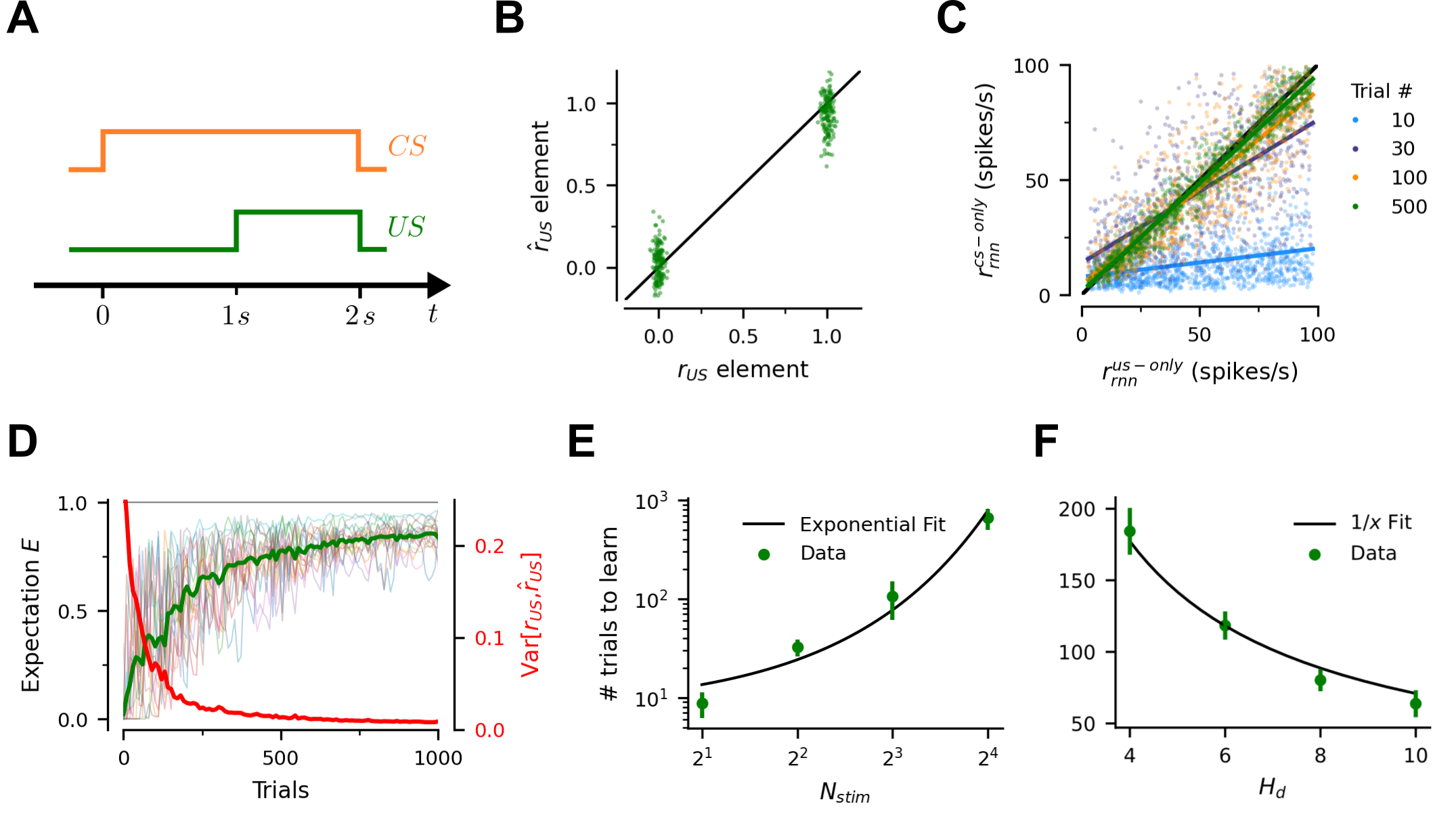
Figure 2: Delay conditioning and stimulus substitution. (A) Trial structure. The network is presented with $N_{\text{stim}}=16$ different CS-US pairs, randomly selected in each trial. (B) The network learns all of the CS-US pairs after 500 training trials ($\approx$ 32 per pair). $r_{\text{us}}$ denotes the individual components of the Boolean vectors encoding each of the USs. $\hat{r}_{\text{us}}$ denotes the individual components of the decoded USs, based only on the presentation of the associated CSs, and measured just before the US appears. (C) Evolution of population responses during learning. Colors denote trial number. Each point compares the firing rate of an associate neuron at that stage of learning for a specific CS-US pair when only the US, or only the associated CS are presented. The colored lines are linear regression fits at each stage of learning. (D) Evolution of predicted US during learning. Green curve depicts the average expectation across USs after the network is presented only with the associated CS. Red curve depicts the distance between the true representation of the USs ($r_{\text{us}}$) and their decoded representation $\hat{r}_{\text{us}}$ when presented only with the associated CS. Individual pairs are shown in faint thin lines. (E) Number of trials required for the network to reach 80% performance for all pairs (defined as the first time at which the average expectation $E$ across pairs exceeds $0.8$) for different numbers of stimulus pairs. Performance is measured just before the US appears. Error bands denote $\mp$ SD computed across 5 different runs of the experiment. (F) Number of trials required to reach 80% performance for all pairs for different levels of similarity in the encoding of the CS and US input vectors. Error bands denote $\mp$ SD computed across 10 different runs of the experiment.

We next investigate how learning evolves with the amount of training. Figure 2C compares the activity of the associative neurons when presented only with the US, for all possible CS-US pairs, with their activity when presented only with the associated CS. Early in training, the associative neurons exhibit little activity in response to the CSs, and their responses are not correlated with the amount of activity elicited by the USs. By the end of training however, the neurons respond to the CS the same way they respond to the US, therefore stimulus substitution is achieved. A host of conditioning phenomena, detailed in following sections, follow from that. For further details on the trial dynamics of learning see the Supplementary Information (section “How does the RNN learn?”). Importantly, in the Supplements we also show that three-factor Hebbian learning rules fail at stimulus substitution in our experiments.

Figure 2D tracks the learning dynamics more closely. The green curve shows the average expectation $E$ assigned to the USs at different stages of training. Perfect learning occurs when $E=1$ for all USs. The red curve provides a measure of distance between the $r_{\text{us}}$ and $\hat{r}_{\text{us}}$. We see that learning requires few repetitions per CS-US, and is substantially faster early on.

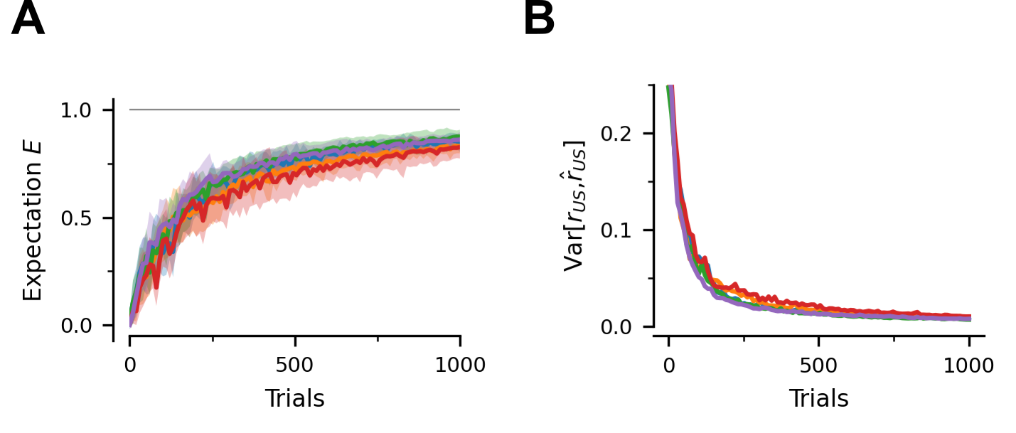
Figure S5: Variation across training runs. Each curve depicts a different training run. Bands represent the $\mp$ SD across stimulus pairs. (A) Expectation for each US after the network is presented only with the associated CS, averaged across all pairs at different levels of training. (B) Distance between the true representation of the USs ($r_{\text{us}}$) and their decoded representation $\hat{r}_{\text{us}}$ when presented only with the associated CS, averaged across all pairs at different levels of training.

There are three sources of randomness in the model: (1) randomness in the sampling of CS and US sets, (2) randomness in the order in which the stimulus pairs are presented, and (3) randomness in the initialization of $W_{\text{rnn}}$, $W_{\text{cs}}$ and $W_{\text{us}}$. In fig. S5 we explore the impact of this noise in our results by training 5 networks with different initializations and training schedules. We find that the level of random variation across training runs is small, and is mostly dominated by randomness in the sampling of the stimuli. For this reason, unless otherwise stated, we present results using only a single training run.

Since the RNN uses mixed representations over the same neurons to encode the stimuli, one natural question is how does learning depend on the number of CS-US pairs in the experiment ($N_{\text{stim}}$) and on the similarity of their representations ($r_{\text{cs}}$ vs $r_{\text{us}}$).

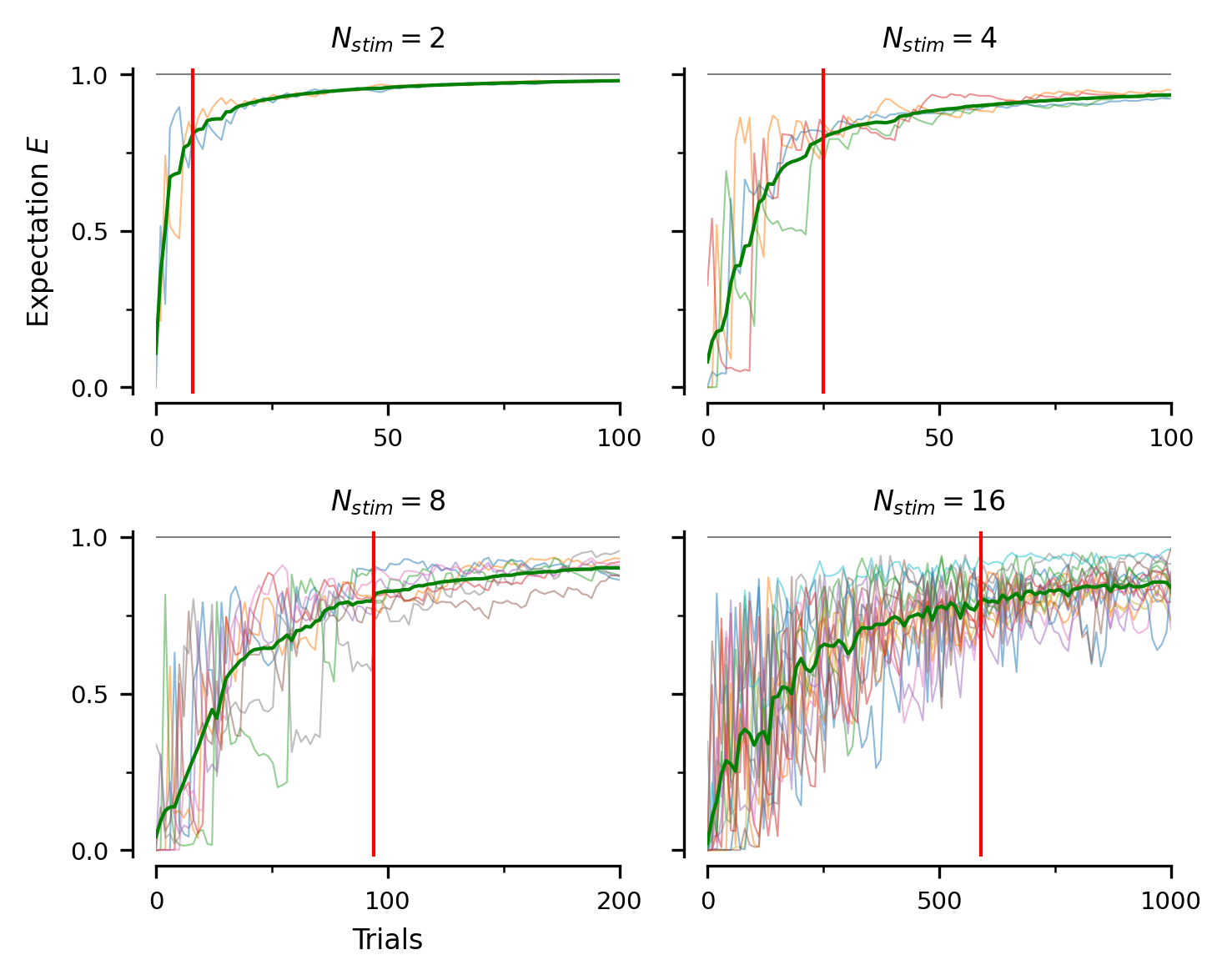
Figure S6: Impact of the number of stimulus pairs on delay conditioning. Learning paths for each CS-US pair for a single experimental run. Each thin line tracks the expectation $E$ for a single stimulus pair. Note that the paths do not increase monotonically, which shows that there can be interference across pairs. The vertical read lines indicate the time at which the average $E$ across pairs (thicker green line) reaches 80% performance level.

We explore the first question by training the model for different values of $N_{\text{stim}}$ and then measuring the number of trials that it takes the network to reach a 80% level of maximum performance, defined as the level of training at which the average expectation $E$ across pairs exceeds $0.8$. Interestingly, the required number of trials increases exponentially with the number of CS-US pairs (fig. 2E). This is likely due to interference across pairs: learning of an association also results in unlearning of other associations at the single trial level. This interference gets worse as the number of stimuli $N_{\text{stim}}$ increases (fig. S6), which might explain the exponential dependence. Finally, note that the network is capable of very fast learning when there are only a few pairs (about 5 presentations per pair for two pairs, fig. 2E).

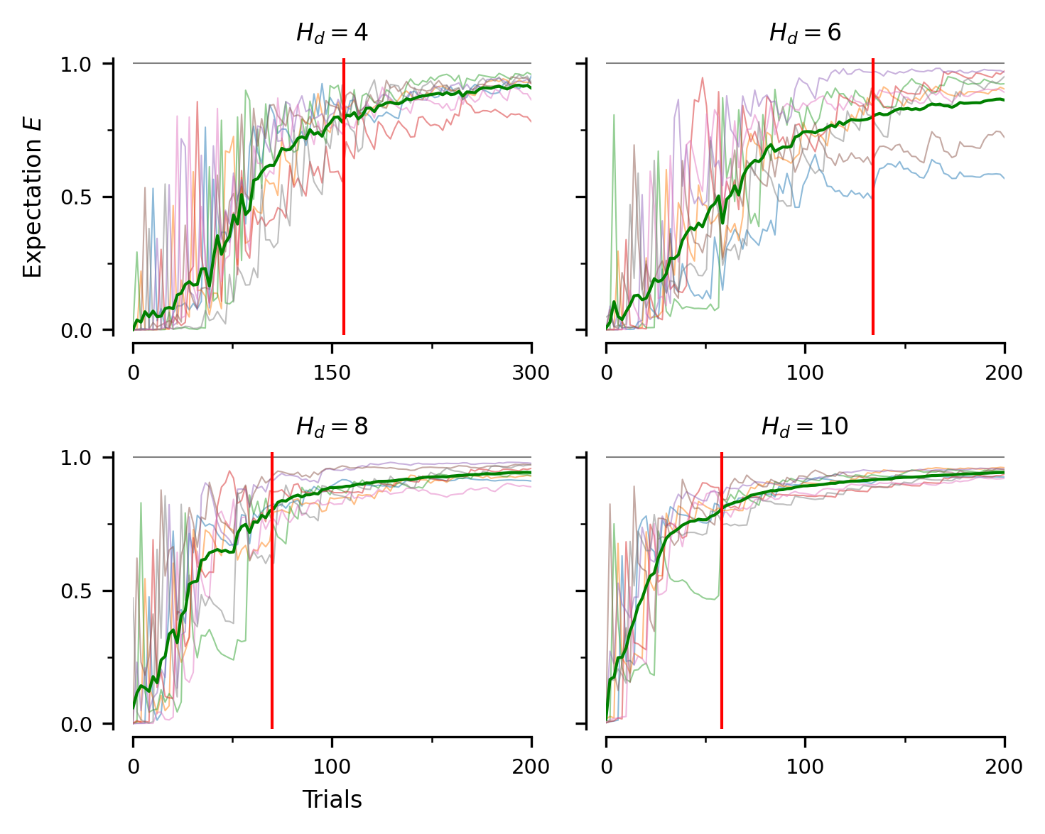
Figure S7: Impact of the similarity on stimulus representation on delay conditioning. Learning paths for each CS-US pair for a single experimental run. Each thin line tracks the expectation $E$ for a single stimulus pair. Note that the paths do not increase monotonically, which shows that there can be interference across pairs. The vertical read lines indicate the time at which the average $E$ across pairs (thicker green line) reaches 80% performance level.

We explore the second question by training the model for different values of the Hamming distances $H_{\text{d}}$, which provides a lower bound on the similarity among USs and, separately, among CSs. $N_{\text{stim}}=8$ for these experiments. Perhaps unsurprisingly, the more dissimilar the stimulus representations, the faster the learning (fig. 2F). Figure S7 shows how smaller $H_{\text{d}}$ naturally leads to greater interference across stimuli.

Short-term memory and trace conditioning

Next we consider trace conditioning experiments, in which there is a delay interval $t_{\text{delay}}>0$ between the disappearance of the CS and the arrival of the US (fig. 3A). In this case the memory network is crucial for maintaining a memory trace of the CS to be associated with the US.

As before, we train the RNN for 1000 trials, with $16$ different pairs, to explore how learning changes over time and how the delay $t_{\text{delay}}>0$ affects learning. For comparison purposes, we include the case of delay conditioning in the same figures ($t_{\text{delay}}=-1$ s).

Figure 3B shows the quality of the decoded representation of the US and fig. 3C-D the strength of the associated expectation signal, both measured offline and in response only to the CS. We find that the RNN learns the associations well for small delays, but that the quality of the learning decays for larger delays. This pattern has been observed in animal experiments [20], and the model provides a mechanistic explanation: conditioning worsens with increasing delays because the memory representation of the CS is leaky and degrades at longer delays, as shown in fig. 1D.

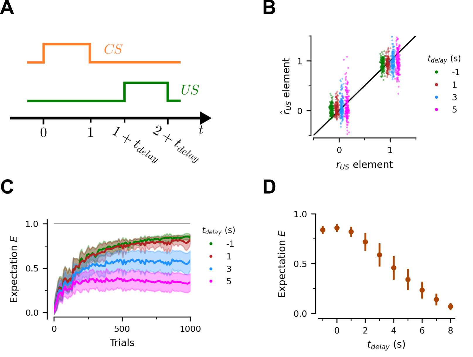
Figure 3: Trace conditioning. (A) Trial structure. The network is presented with $N_{\text{stim}}=16$ different CS-US pairs, randomly selected in each trial. (B) After 500 training trials ($\sim 32$ per pair), the network learns all of the CS-US pairs for short $t_{\text{delay}}$, but struggles for longer delays. $r_{\text{us}}$ denotes the individual components of the Boolean vectors encoding each of the USs. $\hat{r}_{\text{us}}$ denotes the individual components of the decoded USs, based only on the presentation of the associated CSs. For comparison purposes, we also show results for delay conditioning ($t_{\text{delay}}=-1$) (C) Evolution of predicted US during learning. Each curve depicts the expectation for each US after the network is presented only with the associated CS. Line is the mean across all stimulus pairs. Bands represent the $\mp$ SD across stimulus pairs. (D) Network learning performance after 500 training trials for different CS-US delays. Bars denoted $\mp$ SD across stimulus pairs.

Extinction and re-acquisition

The model can also account for the phenomenon of extinction. To investigate this, we focus on the case in which the RNN only needs to learn a single CS-US pair in the delay conditioning task described before. We keep the same trial structure, except that the US is not shown at all, and the trial duration is extended (fig. 4A). The latter is important because in extinction, the computation of surprise in equation 22 is triggered $t_{\text{wait}}$ seconds after the normal time the US would appear, where $t_{\text{wait}}$ is the time after which the US is no longer expected. Without loss of generality, we set $t_{\text{wait}}=5$ seconds.

As shown in fig. 4B, the network learns this association with a small number of trials. At this point the extinction regime is introduced by presenting the same CS in isolation, and as a result the learned association rapidly disappears from the network (fig. 4B,C).

Figure 4D looks at the phenomenon of re-acquisition where, after a period of extinction, the same CS-US pair is reintroduced in training. A common finding in many classical conditioning experiments is that re-acquisition is faster than the initial learning [21]. To test this, we compare two cases: one in which the same US is used during re-acquisition (shown in blue), and one in which a different US is used during re-acquisition (shown in red). We find that re-learning an association to the same US is faster, therefore accounting for experimental findings on re-acquisition. Furthermore, our network provides a mechanistic explanation: re-acquisition is faster because the responses of the neurons in fig. 4C have not decayed to zero, even though the expectation almost has. Therefore, re-learning is faster to begin with, although the new pattern catches up later.

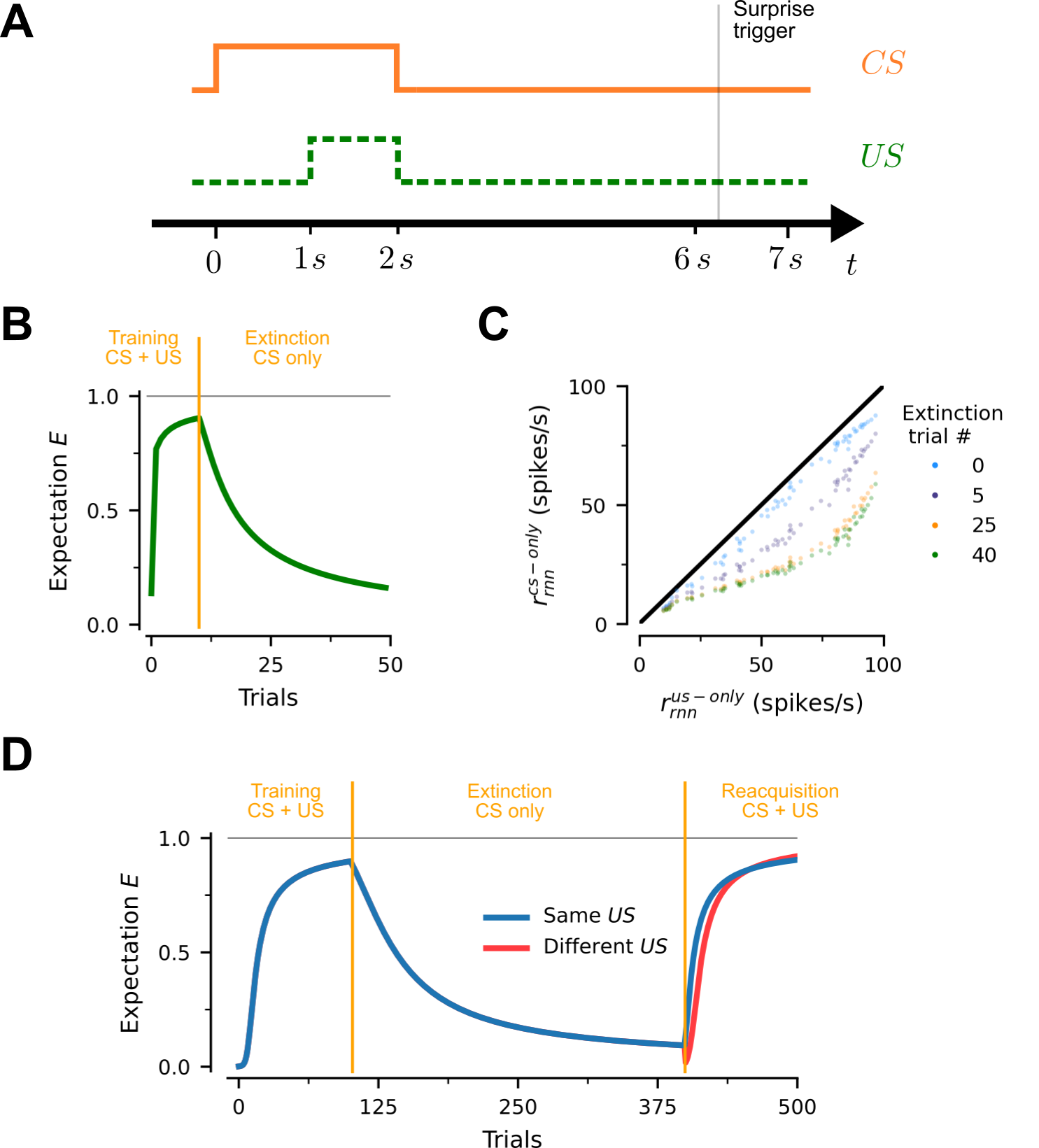
Figure 4: Extinction and re-acquisition. (A) Trial structure. In trials where there US is not shown, surprise is computed at $t\approx 6$ seconds. (B) Learning and extinction path for the acquisition of a single CS-US pair. (C) Evolution of population responses during extinction. Colors denote extinction trial number. Each point compares the firing rate of an associate neuron at that stage of learning for a specific CS-US pair when only the US, or only the associated CS are presented. (D) Learning, extinction and re-acquisition path. Blue line involves an experiment in which the same CS-US pair is used in training and re-acquisition. Red line involves an experiment in which a new US is used at the re-acquisition phase.

Phenomena arising from CS competition

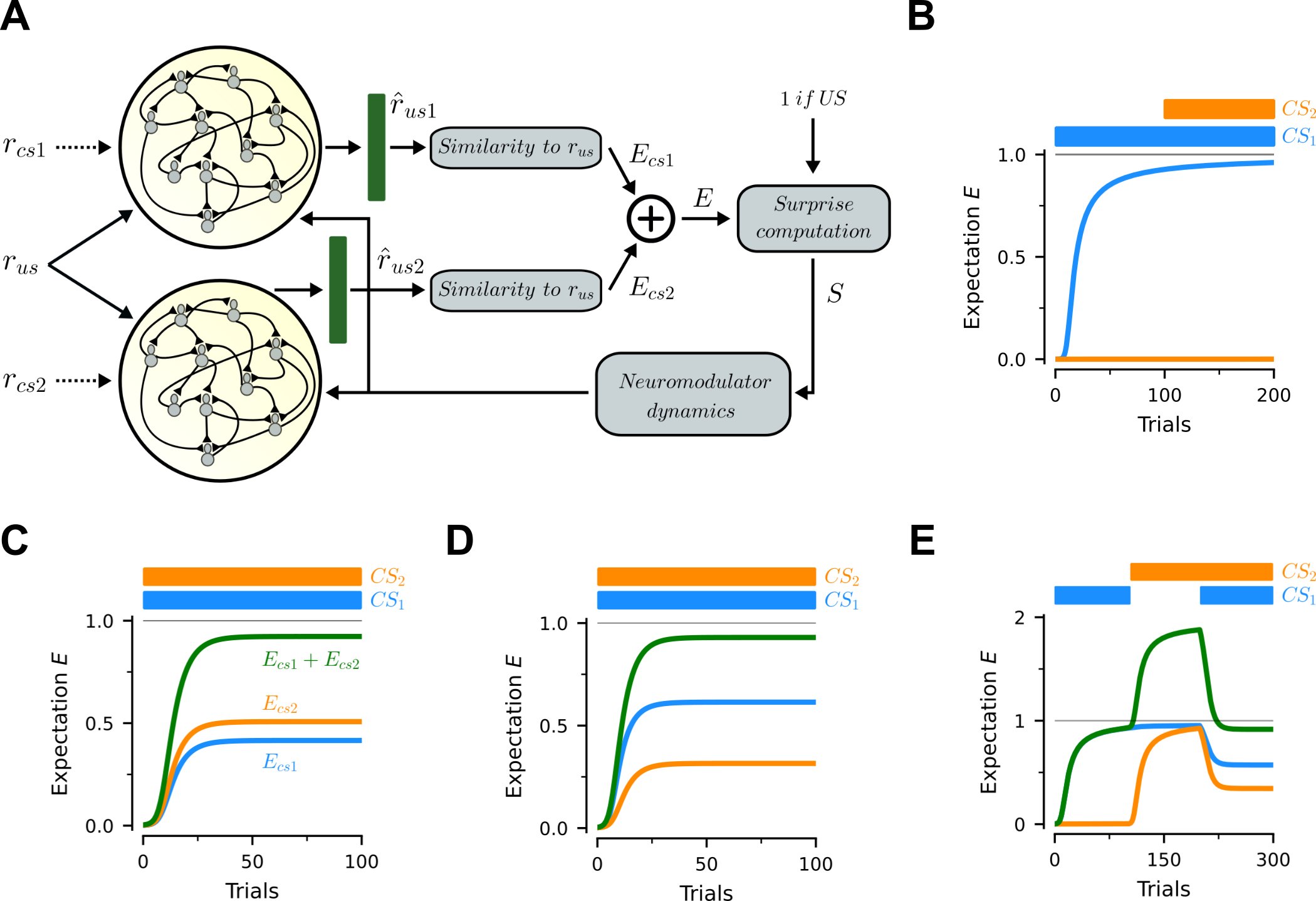
Figure 5: Blocking, overshadowing, saliency and overexpectation. (A) Model extension to allow for simultaneous presentation of two CSs. Associations for $\textit{CS}_{1}$ and $\textit{CS}_{2}$ are represented in separate populations of associative neurons. The activity of each population is used to separately decode the US and to construct expectations $E_{\text{cs1}}$ and $E_{\text{cs2}}$. The overall expectation generated by the two CSs is given by $E=E_{\text{cs1}}+E_{\text{cs2}}$. Experiments assume that a single association between the US and both CSs has to be learnt. $E_{\text{cs1}}$ is the prediction generated by $\textit{CS}_{1}$ alone. $E_{\text{cs2}}$ is the prediction generated by $\textit{CS}_{2}$ alone. and $E_{\text{cs1}}+E_{\text{cs2}}$ is the prediction generated by both cues together. Since the CSs are present throughout the trial, we omit the short-term memory networks from this exercise. (B) Blocking: $\textit{CS}_{1}$ is presented in isolation and fully learns to predict the US before $\textit{CS}_{2}$ is introduced. In this case, $\textit{CS}_{2}$ is blocked from learning to predict the US. (C) Overshadowing: Both CSs are presented from onset and none of them reaches the same conditioning level as when it was presented alone; instead, the sum $E$ of their expectations learns the full association. (D) Saliency effects: similar to (C), but now the relative salience of $\textit{CS}_{1}$ has been increased by scaling up its input vector. As a result, the final conditioning level of $\textit{CS}_{1}$ is consistently higher than the one for $\textit{CS}_{2}$. (D) Overexpectation: $\textit{CS}_{1}$ and $\textit{CS}_{2}$ are conditioned separately. When presented together, $E$ exceeds $1$, which leads to a negative learning rate and unlearning.

So far we have focused on experiments in which the network needs to learn one-to-one CS-US pairings. However, some of the most interesting findings in conditioning arise when multiple CSs are associated with the same US.

To explore this, we extend the model to the case in which the network can be exposed to two CSs for each US (fig. 5A). Now there are two separate RNNs of associative neurons, one for each CS. Without loss of generality we focus on delay conditioning and therefore, for the sake of simplicity, we remove the short-term memory network and directly feed inputs for the respective CSs (denoted by $r_{\text{cs1}}$ and $r_{\text{cs2}}$). The activity of these populations is used to decode the identity of the US, based on the activity generated by each CS separately. These predictions are then used to generate expectations $E_{\text{cs1}}$ and $E_{\text{cs2}}$, which denote the predicted strength generated by each of them when shown in isolation. The total expectation for the US is then given by $E=E_{\text{cs1}}+E_{\text{cs2}}$. The same logic could be extended to more than two CSs. For all of these experiments, we learn a single association between a pair of CSs and a single US, i.e. $N_{\text{stim}}=1$.

Figure 5B presents the results for a typical blocking experiment. We first present $\textit{CS}_{1}$ alone for the first 100 trials, resulting in the acquisition of an expectation very close to $1$. Subsequently, we start presenting both CSs together. However, the US is already well predicted from $\textit{CS}_{1}$, resulting in small surprises after $\textit{CS}_{2}$ is introduced, and thus an approximate zero learning rate. Thus, in this setting the model generates the well established phenomenon of blocking.

Figure 5C studies an overshadowing experiment. Here we present both CSs together from the first trial. In this case both of them develop an expectation from the US, but neither individually reaches $1$. Instead, it is the sum of their expectations that learns the association. Thus, in this setting the model generates the well established phenomenon of overshadowing. Notice that the expectation stemming from one of the CSs is larger than the other, which can be attributed to randomness in the weight matrix initializations.

Figure 5D investigates the impact of stimulus saliency in CS competition. Salient stimuli receive more attention and generate stronger neural responses than similar but less salient ones [22]. We model relative saliency by multiplying the input vector $r_{\text{cs1}}$ of $\textit{CS}_{1}$, the high-saliency cue, by a constant $s_{h}=1.2$, while keeping $r_{\text{cs2}}$ the same. Otherwise, the task is identical to the case of overshadowing. Consistent with animal experiments, fig. 5D shows that the more salient $\textit{CS}_{1}$ acquires a substantially stronger association with the US than the less salient $\textit{CS}_{2}$. This results from the fact that the more salient stimulus leads to higher firing rates, and thus to stronger pre-synaptic potentials which strengthen learning at those synapses.

Finally, fig. 5E presents the results for a typical overexpectation experiment. Here $\textit{CS}_{1}$ is presented alone for the first 100 trials, $\textit{CS}_{2}$ is then presented alone for the next 100, and starting from trial 200, both CSs are presented together. Since at this point the CSs already have expectations very close to $1$, their joint expectation greatly surpasses $1$. As a result, surprise is now negative, leading to unlearning of both conditioned responses, up to the point where $E_{\text{cs1}}+E_{\text{cs2}}\approx 1$.

Contingency and unconditional support

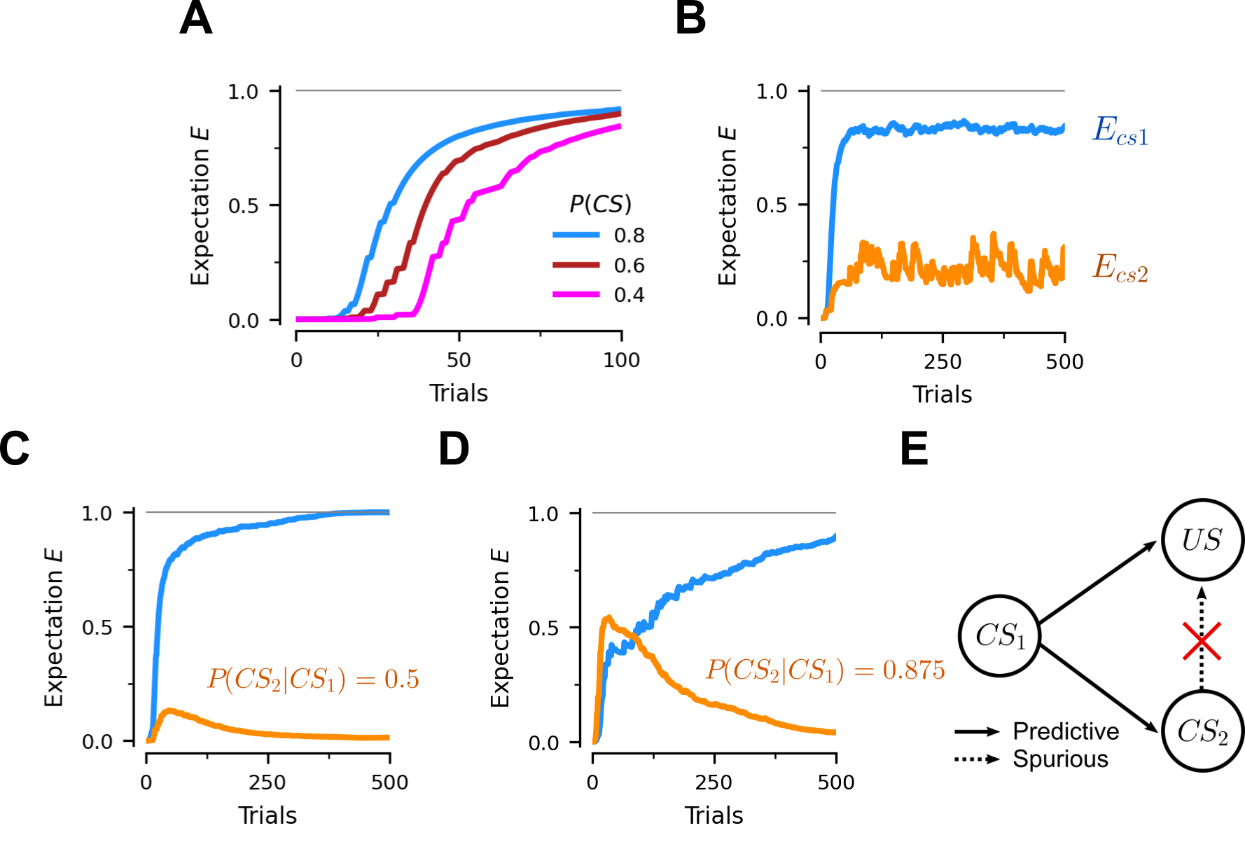
Figure 6: Contingency and causality. The US is shown every trial, while the contingency of the CSs is varied. (A) Impact of changing the probability of showing the CS in every trial. Each line depicts the learning path for a different experiment. (B) Experiment with two independent predictive stimuli. In every trial, $\textit{CS}_{1}$ is shown with probability 0.8 and $\textit{CS}_{2}$ is shown with probability 0.4. Blue curve is the expectation acquired by $\textit{CS}_{1}$ when shown by itself. Orange curve is the expectation acquired by $\textit{CS}_{2}$ when shown by itself. (C,D) Experiments with a conditional CS structure. Every trial $\textit{CS}_{1}$ is shown with probability 0.8 and $\textit{CS}_{2}$ is shown only if $\textit{CS}_{1}$ is also present, with probability $P(\textit{CS}_{2}|\textit{CS}_{1})$. (E) The network learns to ignore spurious predictors. Since $\textit{CS}_{2}$ is conditionally dependent on $\textit{CS}_{1}$, our network gradually phases out any explanatory power of $\textit{CS}_{2}$, as more evidence that the US is never caused by the $\textit{CS}_{2}$ by itself arrives.

So far we have considered experiments that depend on the temporal contiguity of the CS and US. Another important variable affecting conditioning is contingency; i.e., the probability with which the CS and the US are presented together [23].

To vary the level of contingency, the US is shown in every trial, but the CSs are presented only with some probability, which we vary across experiments. Note that this is not the only way of running contingency conditioning experiments. For example, one could change the contingency by showing the CSs every trial and then only show the US with some probability. This would manipulate the degree of contingency, but also introduce an element of extinction, since there are some trials in which no US follows the CS. We favor the aforementioned experiment because it eliminates this confound.

Figure 6A involves experiments with a single CS which is shown with different probability. Consistent with the animal literature [23], we find that the strength and speed of learning increases with the CS-US contingency.

Figure 6B involves experiments with two independent predictive stimuli. Every trial $\textit{CS}_{1}$ is shown with probability 0.8 and, independently, $\textit{CS}_{2}$ is shown with probability 0.4. Unsurprisingly, we find that the CS with the highest contingency acquires the stronger predictive response. Note that the conditioned responses do not need to add up to $1$ in this setting.

Figure 6C,D involves a different probabilistic structure for the CSs. $\textit{CS}_{1}$ is shown every trial with probability 0.8, as in the previous case. But now $\textit{CS}_{2}$ is only shown if $\textit{CS}_{1}$ is present, and with various probability $P(\textit{CS}_{2}|\textit{CS}_{1})$. When $P(\textit{CS}_{2}|\textit{CS}_{1})=0.5$, the unconditional probabilities of the two CSs are the same as in fig. 6B, but the associations learnt are different. After an initial acquisition phase, $E_{\text{cs2}}$ decays monotonically to zero. More interestingly, the same effect arises if $P(\textit{CS}_{2}|\textit{CS}_{1})=0.875$, where $P(CS2)=0.7$: even though the two CSs are similarly likely, $E_{\text{cs2}}$ decays to zero after initially going toe-to-toe with $E_{\text{cs1}}$. This exemplifies the heavily non-linear behavior of this phenomenon.

To explain this finding, we need to introduce the concept of unconditional support. A CS has unconditional support if there are trials when it is presented by itself, which means the network has to rely on it to predict the incoming US. In fig. 6B, both CSs have unconditional support, albeit $\textit{CS}_{2}$’s is much lower. This explains both the noisiness in $E_{\text{cs2}}$, which increases each time $\textit{CS}_{2}$ is presented alone, and the fact that $E_{\text{cs2}}<E_{\text{cs1}}$. However, the situation drastically changes when $\textit{CS}_{2}$ is only presented together with $\textit{CS}_{1}$. Here $\textit{CS}_{2}$ has no unconditional support. Initially, both CSs are conditioned, until the sum of their conditioned responses reaches $1$. At that point no more positive surprise is generated for $\textit{CS}_{2}$. When $\textit{CS}_{1}$ is presented alone, $S>0$ because $E_{\text{cs1}}<1$, which leads to an increase in the $E_{\text{cs1}}$ association. When both CSs are presented together, the sum of their conditioned responses is now greater than $1$, and therefore $S<0$ and both conditioned responses drop. As a result, over time $E_{\text{cs2}}$ gradually decay to zero. This also explain why $E_{\text{cs}}$ takes longer to decay when $P(\textit{CS}_{2}|\textit{CS}_{1})$ is high.

In this task, $\textit{CS}_{2}$ is a spurious predictor of the US, since it only appears if $\textit{CS}_{1}$ is shown, and has no additional predictive value conditional on $\textit{CS}_{1}$, as shown in fig. 6E. Essentially, the network learns to retain the predictive relationship but erase the spurious one. Importantly, we did nothing that would bias the network towards developing this strikingly non-linear effect.

A common fallacy of causal reasoning is known as the post hoc ergo propter hoc fallacy [24]. It posits that the temporal proximity of two events is sufficient to infer that the earlier event is a contributing cause of the latter. This can lead to erroneous conclusions, when such temporal proximity is coincidental. In fig. 6C-E, $\textit{CS}_{1}$ is predictive of both $\textit{CS}_{2}$ and the US, but $\textit{CS}_{2}$ is not predictive of the US, despite it preceding it temporally. Therefore, the network can recognize the lack of predictive ability (or unconditional support) of $\textit{CS}_{2}$, resolving the post hoc fallacy in this simpler predictive setting. Similar mechanisms might allow the brain to perform more advanced forms of causal reasoning.

Finally, note that compared to other conditioning phenomena, the network takes substantially longer to learn the predictive structure of the task. Combined with the fact that real world data are scarce and often ambiguous, this might explain why such fallacies often persist.

Discussion

The ability to engage in stimulus-stimulus associative learning provides a crucial evolutionary advantage. The cerebral cortex might contribute to this evolutionary edge by exploiting representational [7] and architectural [14] inductive biases present in the cortical microcircuit [10]. We here propose a recurrent neuronal network model of how the cortex can implement stimulus substitution, which allows the same set of neurons to encode multiple stimulus-stimulus associations. The model relies on the properties of two-compartment layer-5 pyramidal neurons, which based on recent experimental findings, we refer to as associative neurons. These neurons can act as coincidence detectors for information about the US arriving at their somatic compartment and information about the CS arriving at their dendritic compartment [14, 12, 11]. Coincidence detection allows for a biologically plausible synaptic plasticity rule that, after learning, results in neurons that would normally fire in the presence of the US to respond in the same manner when the CS is presented. At the population level, this means that the pattern of neural activity corresponding to the CS can be morphed into the one corresponding to the US, leading to stimulus substitution.

Our model accounts for many of most important conditioning phenomena observed in animal experiments, including delay conditioning, trace conditioning, extinction, blocking, overshadowing, saliency effects, overexpectation and contingency effects. The model is able to learn multiple CS-US associations with a degree of training that is commensurate with animal experiments. Significantly, the model performs well across a wide variety of conditioning tasks without experiments-specific parameter fine-tuning.

We also show that some influential models of three-factor Hebbian learning rules - Oja’s rule [17] and the BCM rule [18] - fail to learn generic stimulus-stimulus associations due to their unsupervised nature. Hebbian rules have demonstrable autoassociative [25] and heteroassociative [26] capabilities, and when augmented with eligibility traces they have been shown to account for neuronal-level reinforcement learning [16, 27, 28]. Still, they struggle with pattern-to-pattern associations when representations are mixed. This is because Hebbian rules are purely unsupervised, and therefore provide no guarantee that the impact of the CS will be eventually shaped to be identical to the one of the US. Instead, network performance heavily depends on implementation details, like training history, task details and stimulus statistics. As a result, decoding from a population encoding several associations is hampered by the fact that activation levels for individual neurons when exposed to the CS will more often than not be off from those resulting from exposure to the corresponding US.

Related work utilized a predictive learning rule similar to the one used here to account for prospective coding of anticipated stimuli [29]. While prospective coding might also be involved in conditioning, their study differs in several ways. First, their learning rule is timing-dependent; it succeeds in a delayed pair associative learning task, but it would require re-learning when the relative timing of the US in relation to the CS is variable. In contrast, our learning rule applies to arbitrary task timings. Second, their learning rule lacks gating which, unless strict conditions are met (dendritic and somatic activity conditioned on a stationary Markov chain), leads to reduced responses and even catastrophic forgetting. Furthermore, adding gating is not feasible in their model, because learning needs to bootstrap before the presentation of the delayed stimulus, and gating would inactivate learning at these times.

Several features of the model are worth emphasizing.

First, the proposed RNN leverages architectural inductive biases in the form of two-compartment associative neurons. These associative neurons are the most common neuron type in the mammalian cortex [10]. This is likely no coincidence; once evolution stumbled upon their usefulness in predicting external contingencies, it might have favored them. While subcortical [8] and even single-neuron [9] mechanisms for conditioning exist, the mechanism that we propose can handle mixed representations, and thus allow animals with a cerebral cortex to flexibly learn large numbers of associations.

The structure of the associative neuron is ideal for stimulus-stimulus learning. Feedforward inputs, like the US representations, arrive near the soma in layer-5 and directly control the neuron’s firing rate. Feedback inputs, like the CS representations and the activity of other cortical neurons, arrive at the distal dentrites in layer-1 [12]. This compartmentalized structure allows the signals to travel independently, and get associated via a cellular mechanism known as BAC firing [14]. Specifically, it has been shown that these cells implement coincidence detection, whereby feedforward inputs trigger a spike which backpropagates to the distal dendrites and concurrently feedback input arrives at these dendrites, then plateau calcium potentials are initiated in the dendritic compartment [14]. These plateau potentials result in the neuron spiking multiple times subsequently and learning occurs in the distal dendrites, so that feedback inputs can elicit spikes alone in the future, without the need for external information.

Second, a prerequisite for the biological plausiblity of the learning rule used in the model is that backpropagating action potentials to be disentangled from postsynaptic potentials at the dendritic compartment. Only then can the two critical components in our learning rule, $f(V^{\text{s}})$ and $f(p^{\prime}V^{\text{d}})$ in eq. 1 be compared. Since backpropagating action potentials (denoted by $f(V^{\text{s}})$ in the model) do not need to travel far, they experience minimal attenuation [14] and therefore they maintain some of their high-frequency components, which could be used at synapses to differentiate them from slower postsynaptic potentials (denoted by $V^{\text{d}}$ in the model). As a result, only a static transformation of this last term is needed to compare the two signals. Consequently, the learning rule relies only on information locally available at each synapse, which is a prerequisite for biological plausibility.

Third, our model suggests multiple functional roles for gating. It limits learning to episodes that appear to have behavioral significance. Gating also prevents drifting of learned associations due to a lack of perfect self-consistency between $f(V^{\text{s}})$ and $f(p^{\prime}V^{\text{d}})$ in the learning rule [16], which is expected in a biological system subject to noise and approximate computation. In addition, gating provides a critical global reference signal when multiple CSs are available at the same time.

The model also has some limitations to be addressed in future work. Most importantly, it does not account for spontaneous recovery of previously learnt associations after extinction. In our model, extinction stems from the decay of the response of the associate neurons to the CS, a mechanism akin to unlearning, which erases previous learning, and thus does not allow for spontaneous recovery or faster re-acquistion. The extinction mechanism proposed here is complementary to inhibitory learning, the mechanism initially put forth by Pavlov to explain spontaneous recovery.

In the case of experiments with multiple CSs, the model assumes that different neuronal population implements separate RNNs to learn the associations for each of them. Although the two populations interact indirectly through the surprise signals, they each learn to predict the US on their own. The existence of separate populations might be justifiable when the CSs involve different sensory modalities (e.g., sound and vision), or very different spatial locations, but not necessarily when they are presented simultaneously. Extending the model to include differential routing of simultaneously presented stimuli is an open question for future work.

Another direction for future work is to account for more psychological aspects of conditioning by developing a larger model that incorporates other forms of learning and generalization like model-based strategies also thought to take place in the PFC [30], or to allow for context-dependent computation to resolve conflicts among competing stimuli [31]. In these larger models, our network would model the stimulus substitution component.

The model allows to differentiate between conditioning effects that can be accounted by low-level, synaptic plasticity mechanisms, versus other high level explanations. At its core, the model performs stimulus substitution at the neuronal level, via a gradual acquisition process [32, 33, 34]. Despite that, the model is still capable of rapid, few-shot learning, especially when the number of associations is small compared to size of the network (fig. 2E). Yet, for rapid learning in more complicated scenarios, fast inference based on prior knowledge might be necessary [35].

Finally, our model suggest an alternative role for representational inductive biases in the form of mixed selectivity, other than readout flexibility [36]: it permits the efficient packing of multiple stimulus-stimulus associations within the same neuronal population, which might confer cortical animals the evolutionary edge.

Methods

RNN of associative neurons

The central element of the model is a RNN of $N_{\text{rnn}}$ associative neurons. The goal of the network is to learn to predict the identity of the upcoming US from the presentation of the corresponding CS, by reproducing the US population vector when only the CS is presented. Each associative neuron is a two-compartment rate neuron modelled after layer-5 pyramidal cortical neurons [14, 15]. The somatic compartment models the activity of the soma and apical dendrites of the neuron, while the dendritic compartment models the activity of distal dendrites in cortical layer-1. As depicted in fig. 1B, the somatic compartment receives $r_{\text{us}}(t)$ as input, whereas the dendritic compartment receives $\hat{r}_{\text{cs}}(t)$ as well feedback activity from the all the RNN units, which is denoted by $r_{\text{rnn}}(t)$.

The instantaneous firing rate of the associative neurons is a sigmoidal function of the somatic voltage $V^{\text{s}}$:

$$r_{\text{rnn}}=\frac{f_{\text{max}}}{1+\exp\left[-\beta(V^{\text{s}}-V_{1/2})\right]}.$$ (2)

This activation function is applied element-wise to the vector $V^{\text{s}}$, which represents the instantaneous somatic voltage in each associative neuron. $f_{\text{max}}$ sets the maximum firing rate of the neuron, $\beta$ is the slope of the activation function, and $V_{1/2}$ is the voltage level at which half of the maximum firing rate is attained. We set $f_{\text{max}}$ to a reasonable value for cortical neurons, and choose appropriate values for $\beta$ and $V_{1/2}$ so that the whole dynamic range of the activation function is used and firing rates when somatic input is present are relatively uniform. See Table 1 for a description of all model parameters, and Table S1 for their justification.

The somatic voltages, and thus the firing rates, are determined by the following system of differential equations:

• The associative neurons receive an input current to their dendritic compartments, denoted by $I^{\text{d}}$, which obey:

  $$\tau_{\text{s}}\frac{{\textrm{d}}I^{\text{d}}}{{\textrm{d}}t}=-I^{\text{d}}+W_{\text{cs}}\,\hat{r}_{\text{cs}}+W_{\text{rnn}}\,r_{\text{rnn}}$$ (3)

  where $W_{\text{rnn}}$ is the matrix of synaptic weights between any pair of associative neurons (dimension: $N_{\text{rnn}}\times N_{\text{rnn}}$), $W_{\text{cs}}$ is the matrix of synaptic weights for the CS input (dimension: $N_{\text{rnn}}\times N_{\text{inp}}$), and $\tau_{\text{s}}$ is the synaptic time constant.

• The dynamics of the voltage in the dendritic compartments $V^{\text{d}}$ are given by:

  $$\tau_{\text{l}}\frac{\textrm{d}V^{\text{d}}}{\textrm{d}t}=-V^{\text{d}}+I^{\text{d}};$$ (4)

  i.e. it is a low-pass filtered version of the dendritic current $I^{\text{d}}$ with the leak time constant $\tau_{\text{l}}$. For simplicity, voltages and currents are dimensionless in our model. Therefore the leak resistance of the dendritic compartment is also dimensionless and set to unity.

• The voltages of the somatic compartments, denoted by $V^{\text{s}}$, are given by:

  $$C\frac{\textrm{d}V^{\text{s}}}{\textrm{d}t}=-g_{L}V^{\text{s}}-g_{D}(V^{\text{s}}-V^{\text{d}})+I^{\text{s}}$$ (5)

  where $C$ is the somatic membrane capacitance, $g_{L}$ is the leak conductance, $g_{D}$ is the conductance of the coupling from the dendritic to the somatic compartment, and $I^{\text{s}}$ is a vector of input currents to the somatic compartments. Note that this specification assumes that the time constant for the somatic voltage is one, or equivalently, that it is included in $C$.

• The vector $I^{\text{s}}$ of input currents to the somatic compartment is given by:

  $$I^{\text{s}}=g_{\text{e}}\odot(E_{\text{e}}-V^{\text{s}})+g_{\text{i}}\odot(E_{\text{i}}-V^{\text{s}})$$ (6)

  where $g_{\text{e}}$ and $g_{\text{i}}$ are vectors describing the time-varying excitatory and inhibitory conductances of the inputs, $E_{\text{e}}$ and $E_{\text{i}}$ are the reversal potentials for excitatory and inhibitory inputs, and $\odot$ denotes the Hadamard (element-wise) product.

• The vectors of excitatory and inhibitory conductances $g_{\text{e}}$ and $g_{\text{i}}$ for the somatic compartment are described, respectively, by the following two equations:

  $$\tau_{\text{s}}\frac{\textrm{d}g_{\text{e}}}{\textrm{d}t}=-g_{\text{e}}+\left[W_{\text{us}}\right]_{+}r_{\text{us}}$$ (7)

  and

  $$\tau_{\text{s}}\frac{\textrm{d}g_{\text{i}}}{\textrm{d}t}=-g_{\text{i}}+\left[-W_{\text{us}}\right]_{+}r_{\text{us}}+g_{\text{inh}}$$ (8)

  where $W_{\text{us}}$ is a matrix describing the synaptic weights for the US inputs to the somatic compartments (dimension: $N_{\text{rnn}}\times N_{\text{inp}}$), $\tau_{\text{s}}$ is the same synaptic time constant used in equation 3, $g_{\text{inh}}$ is a constant inhibitory conductance of all associative neurons, and $\left[.\right]_{+}$ is the rectification function applied element-wise.

The model implicitly assumes zero resting potentials for the somatic and dendritic compartments. In addition, we assume that there is no input to the RNN between trials, and that the inter-trial interval is sufficiently long so that the variables controlling activity in the associative neurons reset to zero between trials. The differential equations describing activity within trials are simulated using the forward Euler method with time setp $\Delta t=1$ ms.

At the beginning of the experiment, all synaptic weight matrices are randomly initialised, independently for each entry, using a normal distribution with mean 0 and standard deviation $1/\sqrt{N_{\text{rnn}}}$, as is standard in the literature. Note that since associative neurons are pyramidal cells, the elements of $W_{\text{rnn}}$ are restricted to positive values; hence we use the absolute value of those random weights.

$W_{\text{us}}$ stays fixed for the entire experiment. $W_{\text{rnn}}$ and $W_{\text{cs}}$ are plastic and updated using the learning rules described next.

Parameter	Value	Units	Description
$N_{\text{stim}}$	$16$		Number of CS-USs pairs to be learnt
$t_{\text{trial}}$	$2$	s	Trial duration
$t_{\text{cs-off}}$	$2$	s	Time in the trial at which CS disappears
$t_{\text{us-on}}$	$1$	s	Time in the trial at which US appears
$N_{\text{inp}}$	$20$		Stimuli input vector length
$H_{\text{d}}$	$8$		Minimal Hamming distance between behavioral stimulus vectors
$N_{\text{rnn}}$	$64$		Number of associative neurons
$f_{\text{max}}$	$100$	spikes/s	Maximum firing rate
$\beta$	$2$		Steepness of activation function
$V_{1/2}$	$1.5$		Input level for 50 % of the maximum firing rate
$\tau_{\text{s}}$	$100$	ms	Synaptic time constant
$\tau_{\text{l}}$	$20$	ms	Leak time constant of dendritic compartment of associative neurons
$C$	$2$	ms	Capacitance of somatic compartment of associative neurons
$g_{L}$	$0.1$		Leak conductance of somatic compartment of associative neurons
$g_{D}$	$0.2$		Conductance from dendritic to somatic compartment
$g_{\text{inh}}$	$3/8$		Constant inhibitory conductance
$E_{\text{e}}$	$14/3$		Excitatory synaptic reversal potential
$E_{\text{i}}$	$-1/3$		Inhibitory synaptic reversal potential
$a$	$0.95$		Constant for deviation of the learning rule from self-consistency
$\tau_{\text{r}}$	$200$	ms	Dopamine release time constant
$\tau_{\text{u}}$	$300$	ms	Dopamine uptake time constant
$\eta_{0}$	$5*10^{-3}$		Baseline learning rate
$\Delta t$	1	ms	Euler integration step size

Table 1: Model parameter values. These values apply to all simulations, unless otherwise stated. Note that voltages, currents, and conductances are assumed unitless in the text; therefore capacitances have the same units as time constants.

Synaptic plasticity rule

We utilize a synaptic plasticity rule inspired by [14, 12, 11], where the firing rate of the somatic compartment in the presence of the US acts like a target signal for learning the weights $W_{\text{rnn}}$ and $W_{\text{cs}}$ (see [15] for the initial spike-based learning rule, and [37] for the rate-based formulation). The learning rule modifies these synaptic weights so that, after learning, CS inputs can predict the responses of the RNN to the USs.

Consider the synaptic weights from input neuron $j$ to associative neuron $i$, for either the RNN or the CS inputs. The weights are updated continuously during the trial using the following rule:

$$\Delta W_{ij}=\eta(S)\left[\,f(V^{\text{s}}_{i})-f(p^{\prime}\,V^{\text{d}}_{i})\,\right]\,P_{j}$$ (9)

where $\eta(S)$ is a variable learning rate that depends on the instantaneous level of a surprise signal $S$, $p^{\prime}$ is an attenuation constant derived below, and $P_{j}$ is the postsynaptic potential in input neuron $j$.

The postsynpactic potential $P_{j}$ has a simple closed form solution detailed in [37]. In particular, it is a low-passed filtered version of the neuron’s firing rate, so that

$$P_{j}(t)=H(t)*r_{j}(t),$$ (10)

where $*$ denotes the convolution operator, and $H$ is the transfer function given by

$$H(t)=\frac{1}{\tau_{\text{l}}-\tau_{\text{s}}}\left[\exp(-\frac{t}{\tau_{\text{l}}})-\exp(-\frac{t}{\tau_{\text{s}}})\right]u(t)$$ (11)

and $u(t)$ is the Heaviside step function that takes a value of $1$ for $t>0$ and a value of $0$ otherwise.

As noted in [37], for constant $\eta$ the learning rule is a predictive coding extension of the classical Hebbian rule. When $\eta$ is controlled by a surprise signal, as in our model, it can be thought of a predictive coding extension of a three-factor Hebbian rule [28, 38].

Importantly, all of the terms in the learning rule are available at the synapses in the dendritic compartment, making this a local, biologically plausible learning rule. The firing rate of the neuron $f(V^{\text{s}}_{i})$ is available due to backpropagation of action potentials [14]. $f(p^{\prime}V_{i}^{\text{d}})$ is a constant function of the local voltage $V_{i}^{\text{d}}$ computed locally in the dendritic compartment even when the somatic input is present. By definition, postsynaptic potentials are available at the synapse.

There are a total number of $N_{\text{train}}$ training trials, divided among all CS-US pairs. After each training trial we measure the state of the RNN off-line by inputing one $r_{\text{cs}}$ at a time without the US, keeping the network weights constant, and measuring the output produced by the model at that stage of the learning process.

Convergence of synaptic plasticity rule

To understand how and why the learning rule works, it is useful to characterize the somatic voltages, and thus their associated firing rates, in different trial conditions.

Consider first the case in which only the CS is presented, so the associative neurons only receive dendritic input. In this case the somatic voltages converge to a steady-state given by

$$V^{\text{ss}}=\frac{g_{D}}{g_{D}+g_{L}}V^{\text{d}}.$$ (12)

In other words, the somatic voltages converge simply to an attenuated level of the dendritic voltages, with the level of attenuation given by $p=\frac{g_{D}}{g_{D}+g_{L}}$. In this case, the firing rates of the associative neurons converge to

$$r^{\text{cs-only}}_{\text{rnn}}=f(V^{\text{ss}})$$ (13)

This follows from the fact that the dendritic voltage is determined only by equations 3 and 4, and thus is not affected by the state of the somatic compartment, and by the fact that in the absence of US input $I^{\text{s}}=0$. The result then follows immediately from equation 5.

Next consider the case in which only the US is presented. In this case equations 3 and 4 imply that $V^{\text{d}}=0$, and it then follows from equations 5 and 6 that the steady-state somatic voltage, when $I^{\text{s}}=0$, is given by

$$V^{\text{eq}}(t)=\frac{g_{\text{e}}E_{\text{e}}+g_{\text{i}}E_{\text{i}}}{g_{\text{e}}+g_{\text{i}}}$$ (14)

and that the firing rates of the associative neurons become

$$r^{\text{us-only}}_{\text{rnn}}=f(V^{\text{eq}}).$$ (15)

Finally consider the case in which the associative neurons receive input from both the CS and the US. We follow [29] to derive the steady-state solution for the somatic voltage in this case. Provided inputs to the circuit, which are in behavioral timescales, change slower than the membrane time constant ($C/g_{L}=20\,\textrm{ms}$), equation 5 reaches a steady-state given by

$$V^{\text{s}}(t)\approx\kappa V^{\text{ss}}+(1-\kappa)V^{\text{eq}},$$ (16)

where $\kappa(t)=\frac{g_{D}+g_{L}}{g_{D}+g_{L}+g_{\text{e}}+g_{\text{i}}}\in(0,1]$ performs a linear interpolation between the steady-state levels reached where only the CS or the US are presented.

Practically, when there is no US-input, $V^{\text{ss}}$ slightly precedes $V^{\text{s}}$ due to the non-zero dendritic-to-somatic coupling delays, resulting in slight overestimation of the firing rate upon CS presentation. This can be accounted for by introducing an additional small attenuation, so that $p^{\prime}=a\frac{g_{D}}{g_{D}+g_{L}}=ap$ in equation 9, with $a=0.95$.

Learning is driven by a comparison of the firing rates of the associative neurons in the presence of both the CS and the US, and the firing rates if they only receive input from the CS. Importantly, this can happen online and without the need for separate learning phases, because an estimate of the latter can be formed in the dendritic compartment at all times. Learning is achieved by modifying $W_{\text{rnn}}$ and $W_{\text{cs}}$ to minimize this difference. We can use the expressions derived in the previous paragraphs to see why the synaptic learning rule converges to synaptic weights for which $r^{\text{cs-only}}_{\text{rnn}}=r^{\text{both}}_{\text{rnn}}$.

Take the case in which associative neurons underestimate the activity generated by the US inputs when exposed only to the CS (i.e. $V^{\text{ss}}<V^{\text{eq}}$). In this case, $V^{\text{ss}}<V^{\text{s}}<V^{\text{eq}}$ and $I^{\text{s}}>0$. Then from equation 9 we find that $\Delta w>0$, leading to a futures increase in associative neuron activity in response to the CS.

The same logic applies in opposite case, where the associative neurons overestimate the activity generated by the US inputs when exposed only to the CS. In this case, $V^{\text{ss}}>V^{\text{s}}>V^{\text{eq}}$ and $I^{\text{s}}<0$, which leads to a future decrease in associative neuron activity in response to the CS.

Given enough training, this leads to a state where $V^{\text{ss}}\approx V^{\text{eq}}$ and at which learning stops ($\Delta w\approx 0$). When this happens, we have that

$$r^{\text{cs-only}}_{\text{rnn}}=f(V^{\text{ss}})\approx f(V^{\text{eq}})=r^{\text{both}}_{\text{rnn}},$$ (17)

so that the RNN responses to the CS become fully predictive of the activity generated by the US, when presented by themselves.

US decoding

Up to this point the model has been faithful to the biophysics of the brain. The next part of the model is designed to capture the variable learning rate $\eta$ in equation 9, and thus is more conceptual in nature. Our goal here is simply to provide a plausible model of the factors affecting the learning rates for the RNN. As illustrated in fig. 1C, this part of the model involves three distinct computations: decoding the US from the RNN activity, computing expectations about upcoming USs, and computing the surprise signal $S$.

The brain must have a way to decode the upcoming US, or its presence, from the population activity in the RNN at any point during the trial. This prediction is represented by the time-dependent vector $\hat{r}_{\text{us}}(t)$. For the purposes of our model, we will use the optimal linear decoder $D$ (dimension: $N_{\text{rnn}}\times N_{\text{inp}}$), so that

$$\hat{r}_{\text{us}}(t)=r_{\text{rnn}}(t)^{\intercal}D.$$ (18)

The optimal linear decoder $D$ is constructed as follows. First, for each US $i=1,...,N_{\text{stim}}$ define the row vector $\phi_{i}$ describing the steady-state firing rate the each associative neuron that arises when it is presented alone. Then define an activity matrix $\Phi$ by stacking vertically these $N_{\text{stim}}$ row vectors (dimension: $N_{\text{stim}}\times N_{\text{rnn}}$). $\Phi$ is built using the initial random weights $W_{\text{rnn}}$, before learning has taken place. Second, define a target matrix $T$ (dimension: $N_{\text{stim}}\times N_{\text{inp}}$) to be the row-wise concatenated set of US input vectors $r_{\text{us}}$. Then, if $D$ perfectly decodes the US from the RNN activity, when only the USs are presented, we must have that

$$\Phi D=T.$$ (19)

It then follows that

$$D=\Phi^{+}T,$$ (20)

where ⁺ denotes the Moore-Penrose matrix inverse. A desirable property of the Moore-Penrose inverse is that if equation 20 has more than one solutions, it provides the minimum norm solution, which results in the smoothest possible decoding.

Note that the decoder, which could be implemented in any downstream brain area requiring information about USs, is completely independent of the input representations of the CSs. Instead, it is determined before learning given only knowledge of the USs, and is kept fixed throughout training.

US expectation estimation

Since the USs are primary reinforcers, it is reasonable to assume that their representations, $r^{i}_{\text{us}}$ for $i=1,...,N_{\text{stim}}$ , are stored somewhere in the brain. Then an expectation for each US can be formed by

$$E^{i}(t)=\exp(-\kappa\|\hat{r}_{\text{us}}(t)-r^{i}_{\text{us}}\|^{2}),$$ (21)

where $\|\hat{r}_{\text{us}}(t)-r^{i}_{\text{us}}\|$ is Euclidean distance between the stored and the decoded representations for each US at time $t$, and $\kappa$ controls the steepness of the Gaussian kernel. Recognizing that the ability to discriminate these patterns increases with the Hamming distance $H_{\text{d}}$, we set the precision to be inversely proportional to $H_{\text{d}}$ i.e. $\kappa=\left(\frac{8}{H_{\text{d}}}\right)^{2}$.

Note that $E^{i}$ takes values between 0 and 1, and equals 1 only when the US is perfectly decoded (i.e., when $\hat{r}_{\text{us}}=r^{i}_{\text{us}}$). Thus, $E^{i}$ can be interpreted as a probabilistic estimate for each US that is computed throughout the trial. To simplify the notation, we denote the expectation for the US associated with the trial as $E$.

Surprise based learning rates

The learning rule in equation 9 is gated by a well-documented surprise signal [19]. This surprise signal diffuses across the brain, and activates learning in the RNN.

For each US the following surprise signal is computed throughout the trial:

$$S^{i}(t)=\delta(t-t_{\text{trig}})\,\bigl{(}\mathbbm{1}_{US^{i}}-E^{i}(t-t_{\text{syn}})\bigr{)},$$ (22)

where $\mathbbm{1}_{US^{i}}$ is an indicator function for the presence of US-i, $\delta$ is the Dirac delta function and $t_{\text{trig}}$ the time a surprise signal is triggered. In trials where the US appears, we set $t_{\text{trig}}=t_{\text{us-on}}+t_{\text{syn}}$, where $t_{\text{syn}}=2*\tau_{\text{s}}=200\,\textit{ms}$ is a synaptic transmission delay for the detection of the US which matches well perceptual delays [39]. The expectation $E^{i}$ also lags by the same amount, representing synaptic delays from the associative network to the surprise computation area. As can be seen in eq. 22, the more the US is expected upon its presentation, the lower the surprise. In extinction trials, we set $t_{\text{trig}}=t_{\text{us-on}}+t_{\text{syn}}+t_{\text{wait}}$, where $t_{\text{wait}}$ is a time after which a US is no longer expected to arrive. The overall surprise signal is given by:

$$S=\sum_{i}S^{i}.$$ (23)

The surprise signal $S$ gives rise to neuromodulator release and uptake which determine the learning rate $\eta$. We assume that separate neuromodulators are at work for positive and negative surprise, and that they follow double-exponential dynamics [40].

Consider the case of positive surprise. The released and uptaken neuromodulator concentration $C^{+}_{\text{r}}$ and $C^{+}_{\text{u}}$ are given by:

$$\tau_{\text{r}}\frac{\textrm{d}C^{+}_{\text{r}}}{\textrm{d}t}=-C^{+}_{\text{r}}+\left[S\right]_{+}$$ (24)

and

$$\tau_{\text{u}}\frac{\textrm{d}C^{+}_{\text{u}}}{\textrm{d}t}=-C^{+}_{\text{u}}+C^{+}_{\text{r}}$$ (25)

where $\tau_{\text{r}}$ and $\tau_{\text{u}}$ are the neuromodulator release and uptake time constants respectively, chosen to match the dopamine dynamics in fig. 1B in [40].

Negative surprise is controlled by a different neuromodulator, described by the following analogous dynamics:

$$\tau_{\text{r}}\frac{\textrm{d}C^{-}_{\text{r}}}{\textrm{d}t}=-C^{-}_{\text{r}}+\left[-S\right]_{+}$$ (26)

and

$$\tau_{\text{u}}\frac{\textrm{d}C^{-}_{\text{u}}}{\textrm{d}t}=-C^{-}_{\text{u}}+C^{-}_{\text{r}}$$ (27)

The neuromodulator uptake concentrations control the learning rate:

$$\eta=\eta_{0}\ (C^{+}_{\text{u}}-C^{-}_{\text{u}}),$$ (28)

where $\eta_{0}$ is the baseline learning rate.

CS short-term memory circuit

We now describe the short-term memory network used to maintain the $\hat{r}_{\text{cs}}$ representation that serves as input to the RNN.

To obtain a circuit that can maintain a short-term memory through persistent activity in the order of seconds [41], we train a separate recurrent neural network of point neurons using backpropagation through time (BPTT). These networks have been deemed to not be biologically plausible (although see [42]). However, for the purposes of our model we are only interested in the end product of a short-term memory circuit, and not in how the brain acquired such a circuit. Thus, BPTT provides an efficient means of accomplishing this goal.

The memory circuit contains 64 neurons, and the vector of their firing rates $r_{\text{mem}}$ obeys:

$$\tau_{\text{s}}\frac{{\textrm{d}}r_{\text{mem}}}{{\textrm{d}}t}=-r_{\text{mem}}+\left[W_{\text{mem}}\,r_{\text{mem}}+W_{\text{inp}}\,r_{\text{cs}}+b+n_{\text{mem}}\right]_{+}$$ (29)

where $W_{\text{mem}}$ is a matrix with the connection weights between the memory neurons (dimension: $64\times 64$), $W_{\text{inp}}$ is a matrix of connection weights for the incoming CS inputs to the memory net (dimension: $64\times N_{\text{inp}}$), $\tau_{\text{s}}$ is the same synaptic time constant described above, $b$ is a unit-specific bias vector, and $n_{\text{mem}}$ is a vector of IID Gaussian noise with zero mean and variance 0.01 added during training. A linear readout of the activity of the memory network provides the memory representation:

$$\hat{r}_{\text{cs}}=W_{\text{out}}\,r_{\text{mem}},$$ (30)

where $W_{\text{out}}$ is a readout matrix (dimension: $N_{\text{inp}}\times 64$).

The weight matrices $W_{\text{mem}}$, $W_{\text{inp}}$, and $W_{\text{out}}$, as well as the bias vector $b$, are trained as follows. Every trial lasts for 3 seconds. On trial onset, a Boolean vector $r_{\text{cs}}$ is randomly generated and provided as input to the network. The CS input is provided for a random duration drawn uniformly from $\left[0.5,2\right]$ seconds. The network is trained to output $r_{\text{cs}}$ at all times for trials that are 3 seconds long. We train the network for a total of $10^{7}$ trials in batches of 100. We use mean square error loss at the output, with a grace period 200 ms at the beginning of the trial where errors are not penalised. We optimise using Adam [43] with default parameters (decay rates for first and second moments $0.9$ and $0.999$ respectively, learning rate $0.001$). To facilitate BPTT, which does not scale well with the number of timepoints, we train the memory network using a time step of $10*\Delta t$.

Acknowledgements

A.R. gratefully acknowledges support from the NOMIS foundation and from NIH grant R01MH134845. P.V. gratefully acknowledges support from the Onassis Foundation. P.V. would like to thank John O’Doherty whose class was an initial inspiration for this project. No competing interests to disclose.

Author contributions

P.V. conceived the project, developed the model, performed analyses and wrote the initial draft of the manuscript. A.R. supervised the research and provided funding. A.R. and P.V. wrote the final version of the manuscript.

Data and code availability

All code along with data to replicate the results will be shared upon acceptance.

Supplemental Information

How does the RNN learn?

In the main text, we’ve shown that the network is able to learn complex delay conditioning tasks using relatively few trials. In this section we explore in more detail the mechanisms through which the network solves the problem.

Figure S1 shows how the activity of the associative neurons changes with training. It compares firing rates in response only to the CSs (top), in response only to the associated USs (middle), or in response to the full trial in which both are presented (bottom). Several things are worth noticing.

First, the right column depicts the activity of the network after it has learnt the delay conditioning task. At this stage, the activity patterns in response to only the CS or only the US are very similar. This makes it possible to decode the upcoming US using only the activity in the network in response to the associated CS.

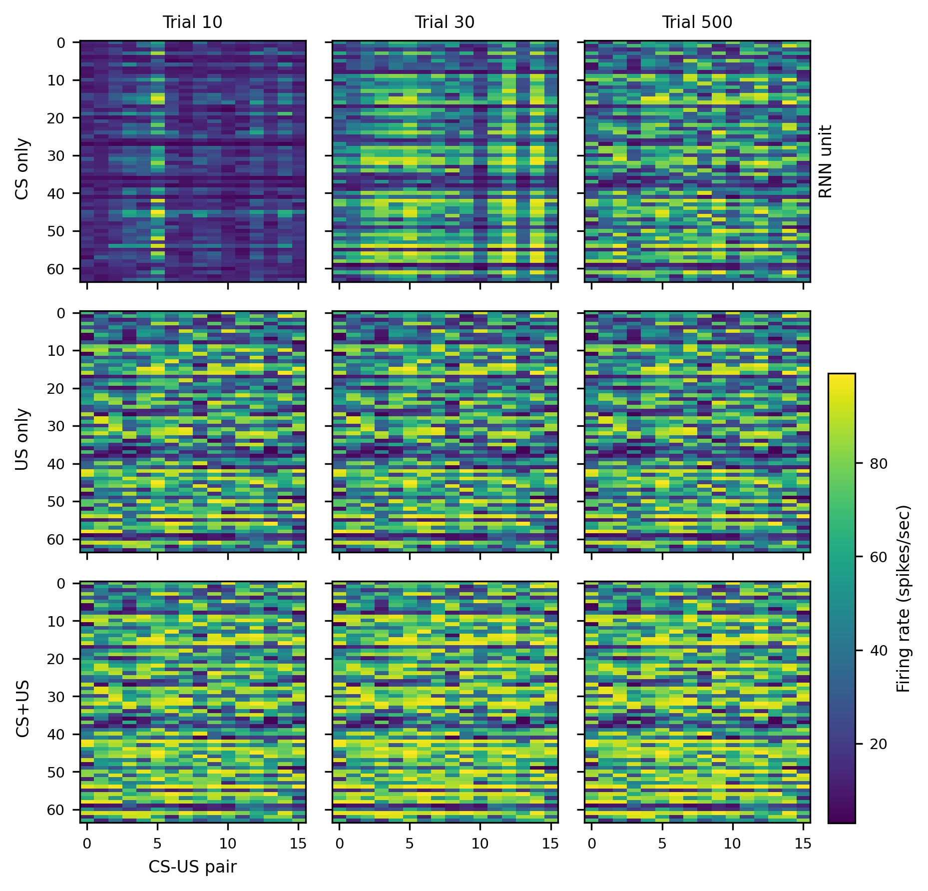
Figure S1: RNN activity during learning. Firing rates in response to each stimulus pair at different stages of learning. Top row shows activity in response only to the associated CS. Middle row shows activity in response only to the associated US. Bottom row shows activity in response to the presentation of both. Activity is measured off-line (i.e., between learning trials).

Second, the network learns mixed stimulus representations. This is important since there is evidence that the associative areas of the prefrontal cortex use this type of mixed coding [7].

Third, the pattern of activity in response to only the US is unchanged by learning. This follows from the fact that in this case the response of the associative neurons is driven only by the input $r_{\text{us}}$ to the somatic compartment and the synaptic weights $W_{\text{us}}$ are not updated with training.

Fourth, the activity pattern in response to both the CS and the US, is very similar to the response to the US alone, irrespective of the stage of learning. This is because the firing rate in our model is mainly controlled by the US, while later in learning the CS would induce the same response anyway. Overall, the learning rule modifies the CS weights so that the CS inputs are able to generate the representation of the US both when the CS is presented by itself, and when presented together with the US.

Figure S2 provides further insight into the inner workings of the model. Each panel depicts the dynamics of a model component within a training trial. Columns denote different stages of training. Recall that the learning rule between associative neuron $i$ and input neuron $j$ is the product of three terms: a surprise modulated learning rate $\eta(S)$, the presynaptic potential in the input neuron $P_{j}$, and the neuron-specific firing rate error term $\left[\,f(V^{\text{s}}_{i})-f(p^{\prime}\,V^{\text{d}}_{i})\,\right]$.

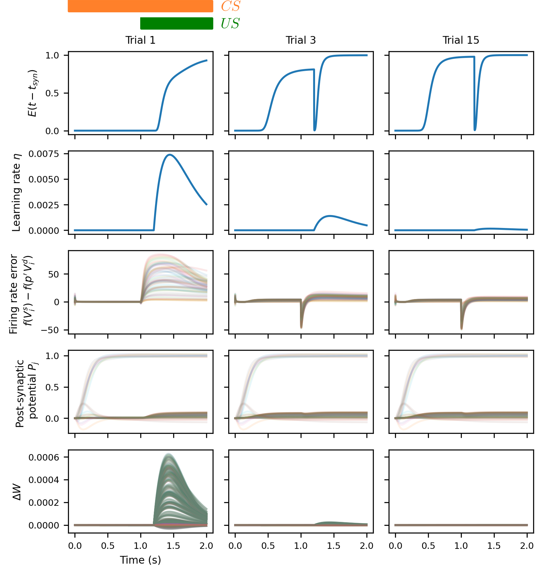
Figure S2: Within trial dynamics of model components. Each panel depicts the dynamics of a model component within a training trial. Columns denote the level of training. Rows denote model variables. $f(V^{\text{s}}_{i})$ is the firing rate of associative neuron $i$, which is determined by its somatic voltage $V^{\text{s}}_{i}$. $f(p^{\prime}V^{\text{d}}_{i})$ is the (approximate) counterfactual firing rate of the neuron when only the CS is presented. $E$ is the expectation signal for the US shown in the trial. $\eta(S)$ is the surprise-modulated learning rate. $P_{j}$ is the presynaptic potentials of input neuron $j$. $\Delta W$ is the incremental weight change for elements of each element in $W_{\text{rnn}}$ and $W_{\text{cs}}$.

Consider the last term first. $f(V^{\text{s}}_{i})$ is the firing rate of associative neuron $i$, which is determined by its somatic voltage $V^{\text{s}}_{i}$. $f(p^{\prime}\,V^{\text{d}}_{i})$ is the (approximate) counterfactual firing rate that would occur if the CS were presented by itself. When the US is presented it dominates the activity of the associative neurons and thus the firing rate in the presence of both stimuli is similar to what would have been in the presence of only the US. As a result, for the RNN to be able to predict the US in response to only the CS, it has to be the case that $f(p^{\prime}\,V^{\text{d}}_{i})\approx f(V^{\text{s}}_{i})$. The learning rule implements a gradient like rule by increasing the CS input weights when $f(p^{\prime}\,V^{\text{d}}_{i})<f(V^{\text{s}}_{i})$, and decreasing them when the opposite is true. As shown in the third row of fig. S2, these two variables are unrelated early in training, but converge to the same pattern as learning progresses.

Next consider the surprise modulated learning rate $\eta(S)$. Gating the learning rate by surprise is critical, as it provides a global reference signal crucial when there are more than one predictive CSs available. Furthermore, biological neurons may not be able to compute $f(p^{\prime}\,V^{\text{d}}_{i})$ exactly at the dendritic compartment, resulting in potential mismatches between $f(V^{\text{s}}_{i})$ and $f(p^{\prime}\,V^{\text{d}}_{i})$. If the learning rate $\eta$ were constant across training, these mismatches would result in slow unlearning when nothing behaviorally significant is happening. In contrast, when the learning rate is gated by surprise, the learning rate $\eta=0$ most of the times, and any mismatch between when $f(V^{\text{s}}_{i})$ and $f(p^{\prime}V^{\text{d}}_{i})$ does not result in unlearning.

Finally consider the presynaptic potential $P_{j}$. This term is present in most learning rules and reflects the old Hebbian dictum that “neurons that fire together wire together”. In particular, other things being equal, the weights of more active synapse are updated more since they have a potentially stronger influence on the postsynaptic firing rate.

We emphasize again that the fact that associative neurons are two-compartment neurons is important for the biological plausibility of the model. The gradient like term $\left[\,f(V^{\text{s}}_{i})-f(p^{\prime}\,V^{\text{d}}_{i})\,\right]$ depends only on information available at the synapse, since it is based only on variables associated with that neuron. By definition, the presynaptic potential $P_{j}$ is also available at the synapse. Finally, the learning rate is implemented by neuromodulators that are diffused to the synapses of the associative network. As a result, all of the variables required to implement the learning rule are locally available at each synapse.

Three-factor Hebbian learning fails at stimulus substitution

The results in the main text have shown that our model accounts for many common patterns in classical conditioning when the RNN is trained with the predictive learning rule in equation 9. A key feature of this rule is that learning is guided by a comparison of activity in the dendritic and somatic compartments of the associative neurons.

In this section we investigate the influence of the learning rule by asking whether the same network trained using previously proposed Hebbian plasticity rules is able to account for the same phenomena. To do this, we keep all of the model components unchanged except for the learning rule. We train the model with two widely used Hebbian-like plasticity rules, Oja’s rule [17] and the BCM rule [18]. We find that the resulting network either cannot learn multiple associations, or requires task specific parameter tuning.

Consider Oja’s learning rule first. In this case the synaptic weights from input neuron $j$ to associative neuron $i$ are updated using the following rule:

$$\Delta W_{ij}=\eta(S)f(V^{\text{s}}_{i})\left[\,P_{j}-nW_{ij}f(V^{\text{s}}_{i})\right]\,$$ (31)

where $n$ is the normalization strength. The normalization component is crucial, because otherwise learning would diverge. Normalization here focuses on the weights, and subjects the largest weights to the strongest normalization. We choose $n=40$ for which the final responses to the CS span most of the output range of associative neurons in our model ($0-100\,\textrm{spikes/s}$).

Figure S3 shows the results of training the RNN with this learning rule in the delay conditioning task. We find that the network can learn well when there is a single CS-US pair, but it fails when it has to learn multiple associations. In fact, $r^{\text{us-only}}_{\text{rnn}}$ and $r^{\text{cs-only}}_{\text{rnn}}$ are anti-correlated in this case. This occurs because normalization introduces competition between incoming synapses to the same neuron [44], which in turn induces competition between the associations to be stored and leads to interference. More specifically, neurons that fire strongly for one pattern will sustain the harshest normalization in their incoming weights affecting the response to all other patterns. Fig. S4A also explores the role of the normalization coefficient and shows that its impact is minimal when learning a single association. This might be because final weight levels for active neurons are determined mostly by the firing rate $f(V^{\text{s}}_{i})$ which is constant for the same association, and hence it serves as a modulator of the learning rate.

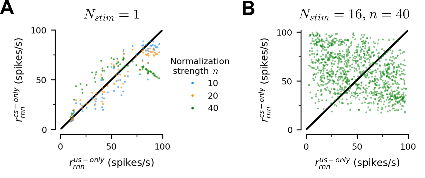
Figure S3: Delay conditioning with Oja’s rule. Each point compares the firing rate of an associative neuron at that stage of learning for a specific CS-US pair when only the US, or only the associated CS are presented. Model is trained using Oja’s rule. (A) Model learns stimulus substitution for different normalization strengths when $N_{\text{stim}}=1$. Model trained for 100 trials with $\eta_{0}=2*10^{-4}$. (B) Models fails to learn after 1000 training trials (64 per CS-US pair) when $N_{\text{stim}}=16$. For this experiment, we use $\eta_{0}=10^{-3}$.

Now consider the BCM rule, which involves an alternative normalization strategy that, instead of focusing on the weights, sets a variable potentiation threshold for the postsynaptic firing rate. The rule is given by:

$$\Delta W_{ij}=\eta(S)f(V^{\text{s}}_{i})\left[\,f(V^{\text{s}}_{i})-\alpha\theta_{i}\right]\,P_{j}$$ (32)

where $\theta_{i}$ is a time-varying threshold, and $\alpha$ is a parameter that modulates the size of the threshold. A common choice is to make the threshold a function of the average recent firing rate, which we implement by making it an exponential moving average of the firing rate though the following differential equation:

$$\tau_{\theta}\frac{{\textrm{d}}\theta_{i}}{{\textrm{d}}t}=-\theta_{i}+f(V_{i}^{\text{s}})$$ (33)

where the parameter $\tau_{\theta}$ determines the temporal window of integration. In theory, this approach sounds promising, since if $r^{\text{cs-only}}_{\text{rnn},i}<r^{\text{both}}_{\text{rnn},i}$, then $f(V_{i}^{\text{s}})>\theta_{i}$ leading to potentiation and vice versa, with this logic converging to $r^{\text{cs-only}}_{\text{rnn},i}\approx r^{\text{both}}_{\text{rnn},i}$. However, as we show this is not enough to guarantee the performance of the BCM rule.

Figure S4 shows the results of training the RNN with the BCM rule and $\alpha=1$. We find that with the same trial conditions used for our main results (as shown in fig. 2) the BCM rule generates intermediate amounts of conditioning, as it has a tendency to overshoot. Furthermore, fig. S4B shows that when we change the time at which the US appears conditioning becomes even worse, and that the problem persists for different values of $\tau_{\theta}$. Since the BCM rule has a tendency of underestimating the impact of the CS, we also explored a remedy that involved amplifying the threshold by setting $\alpha=1.05$. Figure S4C shows that this can fix the problem for experiments in which $t_{us-on}=1$ s, but as shown in fig. S4D, the performance of the network is still highly dependent on US timing. This is because the threshold, determined by a moving averaging filter of the firing rate, is highly dependent on trial specifics. Therefore, we conclude that the time-dependent threshold of the BCM rule introduces sensitivity to experimental details that cannot be overcome.

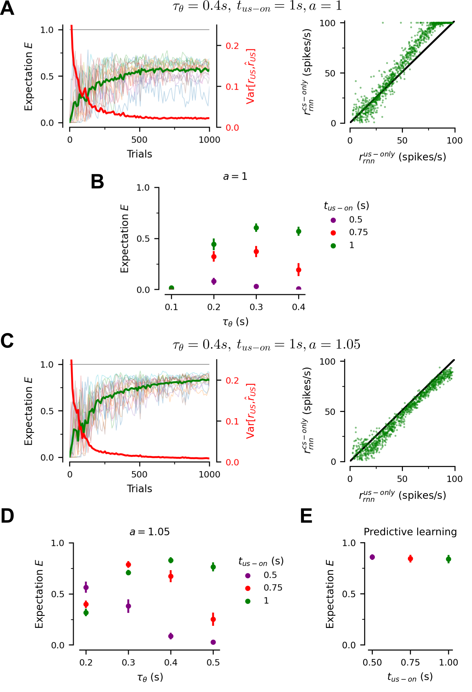
Figure S4: Delay conditioning with BCM rule. Model trained with $\eta_{0}=0.3$ for 1000 trials in order to learn $N_{\text{stim}}=16$ associations. Model parameters and task conditions vary across panels. (A,C) Left: learning path. Green curve depicts the average expectation across CS-USpairs. Learned expectations for individual pairs are shown in faint thin lines. Right: firing rates of all associative neurons after training. (B,D) Network performance, as measured by $E$, as a function of the parameter $\tau_{\theta}$ in the BCM rule and the timing at which the US is presented. (E) Learnt US expectations with our proposed predictive learning rule for different US timings. In contrast to the BCM rule, predictive learning is insensitive to experimental details.

Overall, the need to fine-tune the parameters of the BCM rule to specific trial details is a general problem of Hebbian learning rules, stemming from the fact that they lack supervision. A similar point has been made by [37, 45]. In contrast, predictive learning does not demonstrate such sensitivity. Figure S4E shows that the network learns the task well for a variety of US onset times, without any explicit parameter tuning.

The results in this section showcase the importance of the predictive learning rule in this work, facilitated by the two-compartment nature of the associative neurons. The existence of two compartments, which separate CS inputs to the dendritic compartment from US inputs to the somatic compartment, makes it possible for the biologically plausible learning rule in eq. 9 to compare the two and guide learning using only information locally available at the synapse. In this learning rule, the activity of the somatic compartment serves as a supervisory signal for learning the weights of the inputs to the dendritic compartment until they are able to fully predict their activity in response to the US. In contrast, in this section we have shown that two canonical Hebbian rules struggle with this type of associative learning, in part because they do not have an analogous supervisory signal.

Predictive coding and normative justification for the learning rule

In this section we provide further insight into the learning rule used in our model by showing that it follows directly from the objective of stimulus substitution.

Stimulus substitution states that synaptic connections change during learning so that the activity of the associative network induced by the CS ($r^{\text{cs-only}}_{\text{rnn}}$) becomes identical to the response induced by the US ($r^{\text{us-only}}_{\text{rnn}}$). It follows that the objective of stimulus substitution is to minimize the discrepancy or loss $\mathcal{L}$ between the two:

$$\mathcal{L}=\frac{1}{2}(r^{\text{cs-only}}_{\text{rnn}}-r^{\text{us-only}}_{\text{rnn}})^{2}$$ (34)

We assume that the synaptic weights for US inputs are fixed, since these are primary reinforcers. The synaptic weights for the CS inputs are plastic, and they are shaped so that the CS elicits the same response as the US, essentially becoming predictive of the latter. Assuming a rectified linear (ReLU) activation function, $r^{\text{cs-only}}_{\text{rnn}}$ will obey

$$r^{\text{cs-only}}_{\text{rnn}}=\left[\,W^{\intercal}P\,\right]_{+}$$ (35)

where $W$ are the plastic synaptic weights for the CS inputs, and $P$ are the postsynaptic potentialsof the input CS neurons, low-pass filtered by synaptic delays.

To minimize the loss $\mathcal{L}$, we perform local gradient descent with respect to $W$, which leads to the following update rule:

$$\frac{\partial W}{\partial t}=-\eta\frac{\partial\mathcal{L}}{\partial W}.$$ (36)

This results in the following update rule between input neuron $j$ and associative neuron $i$ from presynaptic neuron $j$:

$$\Delta W_{ij}=\eta\left(r^{\text{us-only}}_{\text{rnn},i}-r^{\text{cs-only}}_{\text{rnn},i}\right)P_{j}.$$ (37)

Here, $r^{\text{us-only}}_{\text{rnn},i}$ acts as a “teacher” signal, in a setting that resembles self-supervised learning. Specifically, $r^{\text{cs-only}}_{\text{rnn},i}$ is compared to $r^{\text{us-only}}_{\text{rnn},i}$, and the discrepancy determines the sign and magnitude of weight change. However, only synapses from presynaptic neurons that have recently been active ($P_{j}>0$) are modified. This learning rule is said to perform predictive coding, because CS inputs should predict (or anticipate) the response to the US.

An implicit requirement of the learning rule is that there has to be a way to tell apart $r^{\text{cs-only}}_{\text{rnn},i}$ and $r^{\text{us-only}}_{\text{rnn},i}$, in order to compare them. However, a neuron only has a single output at a given time. Therefore, in principle it is unclear how the two firing rates could be compared in an online fashion and within the same neuron. The 2-compartment associative neurons resolve this because the activity in the somatic compartment $f(V^{\text{s}}_{i})$ provides a measure of $r^{\text{us-only}}_{\text{rnn},i}$ , $f(p^{\prime}V^{\text{d}}_{i})$ provides a measure of $r^{\text{cs-only}}_{\text{rnn},i}$, and the information available to compute the former term is available in the dendritic compartment due to backpropagating action potentials [14]. Thus, the associative neurons contain all of the information needed to implement the learning rule that yields stimulus substitution.

Supplementary Figures

Parameter	Value	Units	Justification
$N_{\text{stim}}$	$16$		Arbitrary, varied in text
$t_{\text{trial}}$	$2$	s	Arbitrary, varies across experiments
$t_{\text{cs-off}}$	$2$	s	Arbitrary, varies across experiments
$t_{\text{us-on}}$	$1$	s	Arbitrary, varies across experiments
$N_{\text{inp}}$	$20$		Arbitrary
$H_{\text{d}}$	$8$		Arbitrary, varied in text
$N_{\text{rnn}}$	$64$		Larger than number of associations learned
$f_{\text{max}}$	$100$	spikes/s	Matches plausible firing rates
$\beta$	$2$		For smooth change of firing rates as activation varies
$V_{1/2}$	$1.5$		Arbitrary
$\tau_{\text{s}}$	$100$	ms	Taken from literature
$\tau_{\text{l}}$	$20$	ms	Taken from literature
$C$	$2$	ms	Set by $\frac{\tau_{\text{l}}}{g_{L}}$
$g_{L}$	$0.1$		Chosen to be similar in range as somatic conductances from inputs
$g_{D}$	$0.2$		Larger than $g_{L}$ to avoid large coupling attenuation and time lags
$g_{\text{inh}}$	$3/8$		Chosen to get unifrom firing rates distribution
$E_{\text{e}}$	$14/3$		Taken from [15]
$E_{\text{i}}$	$-1/3$		Taken from [15]
$a$	$0.95$		Arbitrary
$\tau_{\text{r}}$	$200$	ms	Fit to experimental data [40]
$\tau_{\text{u}}$	$300$	ms	Fit to experimental data [40]
$\eta_{0}$	$5*10^{-3}$		Chosen for fast learning when $N_{\text{stim}}=1$
$\Delta t$	1	ms	Should be 10 times smaller than smallest time constant

Table S1: Parameter value justifications. These values apply to all simulations, unless otherwise stated. Note that voltages, currents, and conductances are assumed unitless in the text; therefore capacitances have the same units as time constants.

References

- [1] Jenkins HM, Moore BR. The form of the auto-shaped response with food or water reinforcers. Journal of the Experimental Analysis of Behavior. 1973;20(2):163–181. doi:10.1901/jeab.1973.20-163.
- [2] Dai J, Sun QQ. Learning induced neuronal identity switch in the superficial layers of the primary somatosensory cortex; 2023. Available from: http://dx.doi.org/10.1101/2023.08.30.555603.
- [3] Sutton RS, Barto AG. A temporal-difference model of classical conditioning. In: Proceedings of the ninth annual conference of the cognitive science society. Seattle, WA; 1987. p. 355–378.
- [4] Klopf H. A neuronal model of classical conditioning. Psychobiology. 1988;16:85––125. doi:10.3758/BF03333113.
- [5] Balkenius C, Morén J. Computational Models of Classical Conditioning: A Comparative Study; 1998. Available from: http://www.lucs.lu.se/People/Christian.Balkenius/PostScript/LUCS62.pdf.
- [6] Izhikevich EM. Solving the Distal Reward Problem through Linkage of STDP and Dopamine Signaling. Cerebral Cortex. 2007;17(10):2443–2452. doi:10.1093/cercor/bhl152.
- [7] Rigotti M, Barak O, Warden MR, Wang XJ, Daw ND, Miller EK, et al. The importance of mixed selectivity in complex cognitive tasks. Nature. 2013;497(7451):585–590. doi:10.1038/nature12160.
- [8] Christian KM, Thompson RF. Neural Substrates of Eyeblink Conditioning: Acquisition and Retention. Learning & Memory. 2003;10(6):427–455. doi:10.1101/lm.59603.
- [9] Gershman SJ, Balbi PE, Gallistel CR, Gunawardena J. Reconsidering the evidence for learning in single cells. eLife. 2021;10. doi:10.7554/elife.61907.
- [10] Nieuwenhuys R. The neocortex. An overview of its evolutionary development, structural organization and synaptology. Anatomy and Embryology. 1994;190(4). doi:10.1007/bf00187291.
- [11] Doron G, Shin JN, Takahashi N, Drüke M, Bocklisch C, Skenderi S, et al. Perirhinal input to neocortical layer 1 controls learning. Science. 2020;370(6523):eaaz3136. doi:10.1126/science.aaz3136.
- [12] Larkum M. A cellular mechanism for cortical associations: an organizing principle for the cerebral cortex. Trends in Neurosciences. 2013;36(3):141–151. doi:10.1016/j.tins.2012.11.006.
- [13] Shin JN, Doron G, Larkum ME. Memories off the top of your head. Science. 2021;374(6567):538–539. doi:10.1126/science.abk1859.
- [14] Larkum ME, Zhu JJ, Sakmann B. A new cellular mechanism for coupling inputs arriving at different cortical layers. Nature. 1999;398(6725):338–341. doi:10.1038/18686.
- [15] Urbanczik R, Senn W. Learning by the Dendritic Prediction of Somatic Spiking. Neuron. 2014;81(3):521–528. doi:10.1016/j.neuron.2013.11.030.
- [16] Urbanczik R, Senn W. Reinforcement learning in populations of spiking neurons. Nature Neuroscience. 2009;12(3):250–252. doi:10.1038/nn.2264.
- [17] Oja E. Simplified neuron model as a principal component analyzer. Journal of Mathematical Biology. 1982;15(3):267–273. doi:10.1007/bf00275687.
- [18] Bienenstock E, Cooper L, Munro P. Theory for the development of neuron selectivity: orientation specificity and binocular interaction in visual cortex. The Journal of Neuroscience. 1982;2(1):32–48. doi:10.1523/jneurosci.02-01-00032.1982.
- [19] Gerstner W, Lehmann M, Liakoni V, Corneil D, Brea J. Eligibility Traces and Plasticity on Behavioral Time Scales: Experimental Support of NeoHebbian Three-Factor Learning Rules. Frontiers in Neural Circuits. 2018;12. doi:10.3389/fncir.2018.00053.
- [20] Schneiderman N, Gormezano I. Conditioning of the nictitating membrane of the rabbit as a function of CS-US interval. Journal of Comparative and Physiological Psychology. 1964;57(2):188–195. doi:10.1037/h0043419.
- [21] Napier RM, Macrae M, Kehoe EJ. Rapid reacquisition in conditioning of the rabbit’s nictitating membrane response. Journal of Experimental Psychology: Animal Behavior Processes. 1992;18(2):182–192. doi:10.1037/0097-7403.18.2.182.
- [22] Gottlieb JP, Kusunoki M, Goldberg ME. The representation of visual salience in monkey parietal cortex. Nature. 1998;391(6666):481–484. doi:10.1038/35135.
- [23] Rescorla RA. Probability of shock in the presence and absence of cs in fear conditioning. Journal of Comparative and Physiological Psychology. 1968;66(1):1–5. doi:10.1037/h0025984.
- [24] Hamblin CL. Fallacies. London, England: Methuen young books; 1970.
- [25] Hopfield JJ. Neural networks and physical systems with emergent collective computational abilities. PNAS. 1982;79:2554–2558.
- [26] Sompolinsky H, Kanter I. Temporal Association in Asymmetric Neural Networks. Physical Review Letters. 1986;57(22):2861–2864. doi:10.1103/physrevlett.57.2861.
- [27] Vasilaki E, Frémaux N, Urbanczik R, Senn W, Gerstner W. Spike-Based Reinforcement Learning in Continuous State and Action Space: When Policy Gradient Methods Fail. PLoS Computational Biology. 2009;5(12):e1000586. doi:10.1371/journal.pcbi.1000586.
- [28] Frémaux N, Sprekeler H, Gerstner W. Functional Requirements for Reward-Modulated Spike-Timing-Dependent Plasticity. Journal of Neuroscience. 2010;30(40):13326–13337. doi:10.1523/jneurosci.6249-09.2010.
- [29] Brea J, Gaál AT, Urbanczik R, Senn W. Prospective Coding by Spiking Neurons. PLoS Computational Biology. 2016;12(6):e1005003. doi:10.1371/journal.pcbi.1005003.
- [30] Wang JX, Kurth-Nelson Z, Kumaran D, Tirumala D, Soyer H, Leibo JZ, et al. Prefrontal cortex as a meta-reinforcement learning system. Nature Neuroscience. 2018;21(6):860–868. doi:10.1038/s41593-018-0147-8.
- [31] Mante V, Sussillo D, Shenoy KV, Newsome WT. Context-dependent computation by recurrent dynamics in prefrontal cortex. Nature. 2013;503(7474):78–84. doi:10.1038/nature12742.
- [32] Thorndike EL. Animal intelligence: An experimental study of the associative processes in animals. The Psychological Review: Monograph Supplements. 1898;2(4):i–109. doi:10.1037/h0092987.
- [33] Rescorla RA, Wagner AR. A theory of Pavlovian conditioning: Variations in the effectiveness of reinforcement and nonreinforcement. Current research and theory. 1972; p. 64–99.
- [34] Sutton RS, Barto AG. Toward a modern theory of adaptive networks: Expectation and prediction. Psychological Review. 1981;88(2):135–170. doi:10.1037/0033-295x.88.2.135.
- [35] Lake BM, Ullman TD, Tenenbaum JB, Gershman SJ. Building machines that learn and think like people. Behavioral and Brain Sciences. 2016;40:e253. doi:10.1017/s0140525x16001837.
- [36] Fusi S, Miller EK, Rigotti M. Why neurons mix: high dimensionality for higher cognition. Current Opinion in Neurobiology. 2016;37:66–74. doi:10.1016/j.conb.2016.01.010.
- [37] Vafidis P, Owald D, D’Albis T, Kempter R. Learning accurate path integration in ring attractor models of the head direction system. eLife. 2022;11:e69841. doi:10.7554/eLife.69841.
- [38] Frémaux N, Gerstner W. Neuromodulated Spike-Timing-Dependent Plasticity, and Theory of Three-Factor Learning Rules. Frontiers in Neural Circuits. 2016;9. doi:10.3389/fncir.2015.00085.
- [39] Picton TW. The P300 Wave of the Human Event-Related Potential. Journal of Clinical Neurophysiology. 1992;9(4):456–479. doi:10.1097/00004691-199210000-00002.
- [40] Cragg SJ, Hille CJ, Greenfield SA. Dopamine Release and Uptake Dynamics within Nonhuman Primate StriatumIn Vitro. The Journal of Neuroscience. 2000;20(21):8209–8217. doi:10.1523/jneurosci.20-21-08209.2000.
- [41] Wang XJ. Synaptic reverberation underlying mnemonic persistent activity. Trends in Neurosciences. 2001;24(8):455–463. doi:10.1016/s0166-2236(00)01868-3.
- [42] Greedy W, Zhu HW, Pemberton J, Mellor J, Ponte Costa R. Single-phase deep learning in cortico-cortical networks. Advances in Neural Information Processing Systems. 2022;35:24213–24225.
- [43] Kingma D, Ba J. Adam: A Method for Stochastic Optimization. International Conference on Learning Representations. 2014;.
- [44] Gerstner W, Kistler WM, Naud R, Paninski L. Neuronal dynamics. Cambridge, England: Cambridge University Press; 2014.
- [45] Stringer SM, Trappenberg TP, Rolls ET, de Araujo IET. Self-organizing continuous attractor networks and path integration: one-dimensional models of head direction cells. Network: Computation In Neural Systems. 2002;13(2):217–242.