Data Compression using Rank-1 Lattices for Parameter Estimation in Machine Learning

Abstract.

The mean squared error and regularized versions of it are standard loss functions in supervised machine learning. However, calculating these losses for large data sets can be computationally demanding. Modifying an approach of J. Dick and M. Feischl [Journal of Complexity 67 (2021)], we present algorithms to reduce extensive data sets to a smaller size using rank-1 lattices. Rank-1 lattices are quasi-Monte Carlo (QMC) point sets that are, if carefully chosen, well-distributed in a multidimensional unit cube. The compression strategy in the preprocessing step assigns every lattice point a pair of weights depending on the original data and responses, representing its relative importance. As a result, the compressed data makes iterative loss calculations in optimization steps much faster. We analyze the errors of our QMC data compression algorithms and the cost of the preprocessing step for functions whose Fourier coefficients decay sufficiently fast so that they lie in certain Wiener algebras or Korobov spaces. In particular, we prove that our approach can lead to arbitrary high convergence rates as long as the functions are sufficiently smooth.

Keywords: Quasi-Monte Carlo methods, lattice rules, hyperbolic cross, Wiener algebra, Korobov space, supervised learning.

1. Introduction

Let ${\mathcal{X}}=\{{\bm{x}}_{1},\dots,{\bm{x}}_{N}\}\subset[0,1]^{d}$ be a set of data points and ${\mathcal{Y}}=\{y_{1},\dots,y_{N}\}\subset{\mathbb{R}}$ be the corresponding responses. In the context of supervised learning, the goal is to learn a function with a certain structure that maps new data to expected output values. More specifically, we are interested in algorithms that learn parameterized functions $f_{\bm{\theta}}:[0,1]^{d}\to{\mathbb{R}}$ by estimating ${\bm{\theta}}$ using (regularized) least squares approaches. For such approaches, the quantity of interest is the (regularized) mean squared error

(1) $$e(f_{\bm{\theta}},{\mathcal{X}},{\mathcal{Y}})+\lambda r({\bm{\theta}}),$$

where

(2) $$e(f_{\bm{\theta}},{\mathcal{X}},{\mathcal{Y}})=\frac{1}{N}\sum_{n=1}^{N}(f_{\bm{\theta}}({\bm{x}}_{n})-y_{n})^{2}=\frac{1}{N}\sum_{n=1}^{N}f_{\bm{\theta}}^{2}({\bm{x}}_{n})-\frac{2}{N}\sum_{n=1}^{N}y_{n}f_{\bm{\theta}}({\bm{x}}_{n})+\frac{1}{N}\sum_{n=1}^{N}y_{n}^{2},$$

$r({\bm{\theta}})$ is a regularization term to penalize model complexity, and $\lambda>0$ is the regularization strength.

Let us mention some customary choices of regularized errors. As usual, we denote the $\ell^{p}$-norm in ${\mathbb{R}}^{d}$ by $\|\cdot\|_{p}$, i.e., for ${\bm{x}}=[x_{1},\ldots,x_{d}]\in{\mathbb{R}}^{d}$ we have $\left\|{\bm{x}}\right\|_{p}:=\left(\sum_{j\in[d]}\left|x_{j}\right|^{p}\right)^{1/p}$ if $1\leq p<\infty$ and $\left\|{\bm{x}}\right\|_{\infty}:=\max_{j\in[d]}\left|x_{j}\right|$, where $[d]:=\{1,2,\ldots,d\}$. Furthermore, we denote by $\left\|{\bm{x}}\right\|_{0}$ the number of non-zero entries of ${\bm{x}}$. In the case without regularization, i.e., where $r=0$, the loss function in (1) is simply the classical mean squared error as given in (2), which is the standard loss function in simple linear regression, see e.g. [41]. In the case with regularization the following examples of loss functions are commonly used:

1. Loss function for linear regression with the best subset selection $e(f_{{\bm{\theta}}},{\mathcal{X}},{\mathcal{Y}})+\lambda\left\|{\bm{\theta}}\right\|_{0}$, cf. [28, 27].

2. Loss function with lasso penalty $e(f_{{\bm{\theta}}},{\mathcal{X}},{\mathcal{Y}})+\lambda\left\|{\bm{\theta}}\right\|_{1}$, see [42].

3. Loss function for ridge regression with Tikhonov regularization $e(f_{{\bm{\theta}}},{\mathcal{X}},{\mathcal{Y}})+\lambda\left\|T{\bm{\theta}}\right\|_{2}^{2}$, where $T$ is a suitable Tikhonov matrix, cf. [19, 18].

4. Loss function for elastic net regression $e(f_{{\bm{\theta}}},{\mathcal{X}},{\mathcal{Y}})+\lambda\left(\alpha\left\|{\bm{\theta}}\right\|_{1}+(1-\alpha)\left\|{\bm{\theta}}\right\|_{2}^{2}\right)$. This approach tries to find a reasonable balance between the advantages of the ridge regression penalty ($\alpha=0$) and the lasso penalty ($\alpha=1$), see e.g. [16].

Let us emphasize that the data compression approach discussed in this paper works for all regularization functions $r$ in (1), as long as they do not depend on the data points ${\mathcal{X}}$ or the responses ${\mathcal{Y}}$.

The goal is to find parameters ${\bm{\theta}}$ such that the loss function (1) is sufficiently small or even minimal. Now the optimization procedure that is used to calculate suitable parameters ${\bm{\theta}}$ may rely on a large number of evaluations of the loss function; this applies, e.g., for gradient descent algorithms, as well as for general-purpose optimization using one-shot optimization [3], simulated annealing [1], the Nelder-Mead Simplex algorithm [29], or the Broyden-Fletcher-Goldfarb-Shanno algorithm [4, 15, 17, 38]. In this case, the first two sums on the right-hand side of (2) lead to cost that is proportional to the number of evaluations of the loss function times the number $N$ of data points and corresponding responses times the cost of the evaluation of a single function $f_{\bm{\theta}}$. Note that the third sum on the right-hand side of (2) does not depend on ${\bm{\theta}}$ and has to be evaluated at most once, namely if one is interested in the actual values of the errors for different functions $f_{\bm{\theta}}$. If one only wants to find the parameters ${\bm{\theta}}$ that minimize the error function, then the third sum has not to be evaluated at all, since it is independent of ${\bm{\theta}}$ and can be viewed as an additive constant in the objective function. Note furthermore, that the regularization term in (1) does not depend on the data. Since in present-day applications the amount of data is typically very large, Dick and Feischl proposed in [8] the following approach to alleviate the cost burden that is caused by the first two sums on the right-hand side of (2). Let $\nu$ be a positive real number that will be specified later. For $L\ll N$, a suitably chosen point set ${\mathcal{Z}}=\{{\bm{z}}_{0},\dots,{\bm{z}}_{L-1}\}$, and suitably chosen weights $W_{{\mathcal{X}},{\mathcal{Z}},\nu,\ell},W_{{\mathcal{X}},{\mathcal{Y}},{\mathcal{Z}},\nu,\ell}$, we may approximate the mean squared error $e(f_{\bm{\theta}},{\mathcal{X}},{\mathcal{Y}})$ by the following quantity:

(3) $$\operatorname{app}_{L}(f_{\bm{\theta}},{\mathcal{X}},{\mathcal{Y}}):=\frac{1}{L}\sum_{\ell=0}^{L-1}f_{\bm{\theta}}^{2}({\bm{z}}_{\ell})W_{{\mathcal{X}},{\mathcal{Z}},\nu,\ell}-\frac{2}{L}\sum_{\ell=0}^{L-1}f_{\bm{\theta}}({\bm{z}}_{\ell})W_{{\mathcal{X}},{\mathcal{Y}},{\mathcal{Z}},\nu,\ell}+\frac{1}{N}\sum_{n=1}^{N}y_{n}^{2}.$$

Clearly, evaluating $\operatorname{app}_{L}(f_{\bm{\theta}},{\mathcal{X}},{\mathcal{Y}})$ many times for different parameter sets ${\bm{\theta}}$ would be much cheaper than the corresponding evaluations of $e(f_{\bm{\theta}},{\mathcal{X}},{\mathcal{Y}})$. The main question is now, how to choose the point set ${\mathcal{Z}}$ and how to calculate for given data ${\mathcal{X}}$ and ${\mathcal{Y}}$ the corresponding weights $W_{{\mathcal{X}},{\mathcal{Z}},\nu,\ell}$ and $W_{{\mathcal{X}},{\mathcal{Y}},{\mathcal{Z}},\nu,\ell}$? Our priority objective is that $\operatorname{app}_{L}(f_{\bm{\theta}},{\mathcal{X}},{\mathcal{Y}})$ should be a tight approximation of $e(f_{\bm{\theta}},{\mathcal{X}},{\mathcal{Y}})$. Another objective is that the cost of computing the weights should be low. Since we can reuse the (pre-)computed weights in the course of the optimization procedure to calculate the loss function for as many sets of parameters ${\bm{\theta}}$ as we like, this cost can be viewed as precomputation or “start-up” cost. Hence, it would be perfectly in order if this cost is actually not very small, but of some reasonable amount instead.

Dick and Feischl recommended choosing ${\mathcal{Z}}$ as a digital net, which is a quasi-Monte Carlo point set that is uniformly distributed in the unit cube $[0,1]^{d}$, cf. [30, 7]. They showed how to choose the corresponding weights $W_{{\mathcal{X}},{\mathcal{Z}},\nu,\ell}$ and $W_{{\mathcal{X}},{\mathcal{Y}},{\mathcal{Z}},\nu,\ell}$, estimated the cost of their precomputation, and studied the resulting approximation error

(4) $${\rm err}:=|e(f_{\bm{\theta}},{\mathcal{X}},{\mathcal{Y}})-\operatorname{app}_{L}(f_{\bm{\theta}},{\mathcal{X}},{\mathcal{Y}})|.$$

We propose to choose ${\mathcal{Z}}$ as a rank-$1$ lattice, constructed with the help of a fast component-by-component algorithm, see [39, 25, 33]. Similarly as in [8], we derive formulas for the corresponding weights, see Section 2. Furthermore, we estimate the cost of their precomputation and analyze the approximation error of this approach, see Section 3.

We compare both approaches in Section 4. Roughly speaking, the results of the comparison are as follows: On the one hand, we are able to prove for our specific approach convergence rates of approximation errors that are better than the ones obtained in [8]. In particular, the (polynomial) convergence rates derived in [8] are always strictly less than $1$, regardless of the smoothness of the function $f_{\bm{\theta}}$, while our approach leads to convergence rates that essentially increase linearly with the smoothness of $f_{\bm{\theta}}$ and can therefore be arbitrarily large. On the other hand, the cost of precomputing the weights are roughly comparable, but, nevertheless, may be a bit smaller in the case of digital nets. As explained above, the computation of the weights can be viewed as precomputation, which is done before the optimization procedure itself starts. That is why we believe that the (reasonably small) differences in the cost of these computations are not an issue. Nevertheless, as explained at the end of Section 4, we can easily modify our approach and reduce the cost of precomputing the weights if we are ready to accept a reduced convergence rate of the approximation error. With this trade-off we are able to achieve essentially the same cost of precomputation as Dick and Feischl do. For the details, see Section 4.

Let us emphasize that the analysis in [8] as well as the analysis in the main part of our paper do not assume that the models, i.e., the functions $f_{\bm{\theta}}$, have some structure, apart from a certain degree of smoothness, or that the data points ${\mathcal{X}}$ have some specific distribution. If the models or the data points have additional structure, one can try to exploit this. Consider, e.g., the case that the model is a truncated Fourier series

$$f_{{\bm{\theta}}}({\bm{x}}):=\sum_{{\bm{k}}\in K}\theta_{{\bm{k}}}\omega_{{\bm{k}}}({\bm{x}}),$$

where $K$ is a finite subset of ${\mathbb{Z}}^{d}$, $\omega_{\bm{k}}$ are the trigonometric bases functions defined as

$$\omega_{\bm{k}}({\bm{x}}):=\exp\left(2\pi i\cdot{\bm{k}}\cdot{\bm{x}}\right),$$

${\bm{k}}\cdot{\bm{x}}:=\sum_{j=1}^{d}k_{j}x_{j}$ the standard scalar product in ${\mathbb{R}}^{d}$, and ${\bm{\theta}}:=\{\theta_{{\bm{k}}}\}_{{\bm{k}}\in K}$ are the Fourier coefficients (parameters) we want to learn. The Fourier coefficients for a function $f\in L_{1}([0,1]^{d})$ are defined as

$$\widehat{f}_{\bm{k}}:=\int_{[0,1]^{d}}f({\bm{x}})\exp(-2\pi i{\bm{k}}\cdot{\bm{x}}){\,\mathrm{d}{\bm{x}}},\quad{\bm{k}}\in{\mathbb{Z}}^{d}.$$

In this case our lattice rule approach may be particularly beneficial, since evaluating the functions $f_{\bm{\theta}}$ at all the points of a rank-$1$ lattice ${\mathcal{Z}}$ may be done with the help of the univariate fast Fourier transform, regardless of the form of the finite index set $K$, cf. [20]. This leads to a reasonable speed up: While the cost of evaluating $f_{\bm{\theta}}$ in all the points of a general point set ${\mathcal{Z}}$ is of order $O(d|K|L)$, choosing ${\mathcal{Z}}$ as a rank$1$-lattice reduces it to $O(d|K|+L\log(L))$, cf. Section 3.3.2. Truncated Fourier series models are of particular interest in the explainable ANOVA approximation approach in machine learning as introduced in [35] and further developed, e.g., in [36, 37].

Of course, there are approaches known that are different from, but related to the ones proposed by Dick and Feischl and in this paper; for a discussion of relevant algorithms, their convergence rates and cost as well as for references to the literature we refer the reader to Section 1.1 of [8].

Let us finish this introduction by emphasizing that this paper focuses solely on the theoretical analysis of the QMC data compression approach based on lattice point sets. In particular, our main goals are to provide a transparent error analysis that may also be extended to other interesting point sets, and to show that the convergence rates of approximation errors can indeed be arbitrarily high if the input functions are sufficiently smooth. A rigorous study of numerical experiments for interesting use cases is beyond the scope of this paper.

2. Derivation of compression weights

In [8] the authors presented two approaches to deduce formulas for the compression weights from (3) that are suitable for digital nets ${\mathcal{Z}}$. The first approach is based on geometrical properties of digital nets and on an inclusion-exclusion formula. It seems to us that this approach cannot be modified in a reasonable way to work also for lattice point sets. The second approach is based on a truncation of the Walsh series of the functions $f_{\bm{\theta}}$ and $(f_{\bm{\theta}})^{2}$, respectively. As we will show now, this approach can be modified appropriately for lattice point sets ${\mathcal{Z}}$ by considering Fourier series instead of Walsh series. As in [8], we consider a function $g$ and coefficients $c_{n}$, where, in order to derive the weights $W_{{\mathcal{X}},{\mathcal{Z}},\nu,\ell}$ we set

(5) $$g=f_{\bm{\theta}}^{2},\quad c_{n}=1,$$

and for the weights $W_{{\mathcal{X}},{\mathcal{Y}},{\mathcal{Z}},\nu,\ell}$, we set

(6) $$g=f_{\bm{\theta}},\quad c_{n}=y_{n}.$$

Let us assume that the Fourier series of $g$ converges absolutely and uniformly on $[0,1]^{d}$. Let $K\subset{\mathbb{Z}}^{d}$ be a finite subset that will be suitably chosen later. Then we define the function

$$g_{K}:=\sum_{{\bm{k}}\in K}\widehat{g}_{{\bm{k}}}\omega_{{\bm{k}}},$$

where $\widehat{g}_{{\bm{k}}}=\left\langle g,\omega_{{\bm{k}}}\right\rangle_{L^{2}([0,1]^{d})}$ is the ${\bm{k}}$-th Fourier coefficient of $g$. Consequently,

$$g-g_{K}=\sum_{{\bm{k}}\in{\mathbb{Z}}^{d}\setminus K}\widehat{g}_{{\bm{k}}}\omega_{{\bm{k}}}.$$

We want to choose $K$ big enough so that the tail $g-g_{K}$ is small. In other words, we aim to have $g_{K}\approx g$.

Assume that $K=K_{\nu,d}$ depending on a parameter $\nu>0$ such that $\lim_{\nu\to\infty}\left\|g-g_{K_{\nu,d}}\right\|_{\infty}=0.$ Then, from the orthogonality of the functions $\omega_{{\bm{k}}}$ in $L^{2}([0,1]^{d})$ we have

(7) $$\frac{1}{N}\sum_{n=1}^{N}c_{n}g({\bm{x}}_{n}) =\frac{1}{N}\sum_{n=1}^{N}c_{n}g_{K}({\bm{x}}_{n})+\frac{1}{N}\sum_{n=1}^{N}c_{n}(g-g_{K})({\bm{x}}_{n})$$

$$\approx\frac{1}{N}\sum_{n=1}^{N}c_{n}g_{K}({\bm{x}}_{n})=\frac{1}{N}\sum_{n=1}^{N}c_{n}\sum_{{\bm{k}}\in K}\widehat{g}_{{\bm{k}}}\omega_{{\bm{k}}}({\bm{x}}_{n})$$

$$=\int_{[0,1]^{d}}g({\bm{x}})\left(\sum_{{\bm{k}}\in K}\overline{\omega_{{\bm{k}}}({\bm{x}})}\frac{1}{N}\sum_{n=1}^{N}c_{n}\omega_{{\bm{k}}}({\bm{x}}_{n})\right){\,\mathrm{d}{\bm{x}}}$$

$$=\int_{[0,1]^{d}}g({\bm{x}})\phi_{K}({\bm{x}}){\,\mathrm{d}{\bm{x}}},$$

for the function

$$\phi_{K}({\bm{x}}):=\sum_{{\bm{k}}\in K}\widecheck{\phi}_{{\bm{k}}}\overline{\omega_{{\bm{k}}}({\bm{x}})}$$

where the coefficients are

$$\widecheck{\phi}_{{\bm{k}}}:=\frac{1}{N}\sum_{n=1}^{N}c_{n}\omega_{{\bm{k}}}({\bm{x}}_{n}).$$

Let us denote ${\mathcal{C}}:=(c_{n})_{n\in[N]}$. We define the truncation error, obtained from (7), as

(8) $$\operatorname{err}_{1}(g,{\mathcal{C}}) :=\left|\frac{1}{N}\sum_{n=1}^{N}c_{n}g({\bm{x}}_{n})-\int_{[0,1]^{d}}g({\bm{x}})\phi_{K}({\bm{x}}){\,\mathrm{d}{\bm{x}}}\right|=\left|\frac{1}{N}\sum_{n=1}^{N}c_{n}(g-g_{K})({\bm{x}}_{n})\right|$$

$$\leq\left\|(g-g_{K})\right\|_{\infty}\frac{1}{N}\sum_{n=1}^{N}\left|c_{n}\right|.$$

Once $K$ is chosen, we can approximate the last integral in (7) by a suitable quadrature given by points ${\mathcal{Z}}=\{{\bm{z}}_{0},\dots,{\bm{z}}_{L-1}\}$ as follows

(9) $$\int_{[0,1]^{d}}(g\phi_{K})({\bm{x}}){\,\mathrm{d}{\bm{x}}}\approx\frac{1}{L}\sum_{\ell=0}^{L-1}(g\phi_{K})({\bm{z}}_{\ell}).$$

Consequently, we define the approximation error obtained from (9) as

(10) $$\operatorname{err}_{2}(g,{\mathcal{C}}):=\left|\int_{[0,1]^{d}}(g\phi_{K})({\bm{x}}){\,\mathrm{d}{\bm{x}}}-\frac{1}{L}\sum_{\ell=0}^{L-1}(g\phi_{K})({\bm{z}}_{\ell})\right|.$$

Both steps (7) and (9) lead to the approximation

$$\frac{1}{N}\sum_{n=1}^{N}c_{n}g({\bm{x}}_{n})\approx\int_{[0,1]^{d}}g({\bm{x}})\phi_{K}({\bm{x}}){\,\mathrm{d}{\bm{x}}}\approx\frac{1}{L}\sum_{\ell=0}^{L-1}(g\phi_{K})({\bm{z}}_{\ell}).$$

If we follow the approach described above, the weights $W_{{\mathcal{X}},{\mathcal{Z}},\nu,\ell}$ and $W_{{\mathcal{X}},{\mathcal{Y}},{\mathcal{Z}},\nu,\ell}$ in (3) are of the form

(11) $$\phi_{K}({\bm{z}}_{\ell})=\frac{1}{N}\sum_{{\bm{k}}\in K}\sum_{n=1}^{N}c_{n}\omega_{{\bm{k}}}({\bm{x}}_{n}-{\bm{z}}_{\ell}).$$

More precisely, for $g=f_{\bm{\theta}}^{2}$ and $c_{n}=1$, we get the first set of input-dependent weights

$$W_{{\mathcal{X}},{\mathcal{Z}},\nu,\ell}=\frac{1}{N}\sum_{{\bm{k}}\in K}\sum_{n=1}^{N}\omega_{{\bm{k}}}({\bm{x}}_{n}-{\bm{z}}_{\ell}).$$

For $g=f_{\bm{\theta}}$ and $c_{n}=y_{n}$, we get the second set of input-output dependent weights

$$W_{{\mathcal{X}},{\mathcal{Y}},{\mathcal{Z}},\nu,\ell}=\frac{1}{N}\sum_{{\bm{k}}\in K}\sum_{n=1}^{N}y_{n}\omega_{{\bm{k}}}({\bm{x}}_{n}-{\bm{z}}_{\ell}).$$

Remark 2.1.

The total error we are interested in is

$$\left|e(f_{\bm{\theta}},{\mathcal{X}},{\mathcal{Y}})-\operatorname{app}_{L}(f_{\bm{\theta}},{\mathcal{X}},{\mathcal{Y}})\right|\leq \left|\frac{1}{N}\sum_{n=1}^{N}f_{\bm{\theta}}^{2}({\bm{x}}_{n})-\frac{1}{L}\sum_{\ell=0}^{L-1}f_{\bm{\theta}}^{2}({\bm{z}}_{\ell})W_{{\mathcal{X}},{\mathcal{Z}},\nu,\ell}\right|$$

$$+2\left|\frac{1}{N}\sum_{n=1}^{N}y_{n}f_{\bm{\theta}}({\bm{x}}_{n})-\frac{1}{L}\sum_{\ell=0}^{L-1}f_{\bm{\theta}}({\bm{z}}_{\ell})W_{{\mathcal{X}},{\mathcal{Y}},{\mathcal{Z}},\nu,\ell}\right|$$

$$\leq\operatorname{err}_{1}(f_{\bm{\theta}}^{2},{\bm{1}}_{N})+\operatorname{err}_{2}(f_{\bm{\theta}}^{2},{\bm{1}}_{N})+2(\operatorname{err}_{1}(f_{\bm{\theta}},{\mathcal{Y}})+\operatorname{err}_{2}(f_{\bm{\theta}},{\mathcal{Y}})),$$

where ${\bm{1}}_{N}:=(1)_{n\in[N]}$. That is, to estimate the error, it suffices to estimate

(12) $$\left|\frac{1}{N}\sum_{n=1}^{N}c_{n}g({\bm{x}}_{n})-\frac{1}{L}\sum_{\ell=0}^{L-1}(g\phi_{K})({\bm{z}}_{\ell})\right|\leq\operatorname{err}_{1}(g,{\mathcal{C}})+\operatorname{err}_{2}(g,{\mathcal{C}}),$$

for $g$ and $c_{n}$ as in  (5) and (6), $\operatorname{err}_{1}$ as in (8), $\operatorname{err}_{2}$ as in (10), and for $\phi_{K}$ as in  (11).

3. Error and cost analysis

For our error and cost analysis, we consider weighted function spaces with product weights induced by a decreasing sequence of weights $1\geq\gamma_{1}\geq\gamma_{2}\geq...\geq\gamma_{d}>0$ assigned to all the variables. Then the weight (or importance) of a set of interacting variables ${\bm{u}}$ is given by $\gamma_{\bm{u}}=\prod_{j\in{\bm{u}}}\gamma_{j}$ for non-empty ${\bm{u}}$, and we set $\gamma_{\emptyset}=1$. Product weights for weighted function spaces were first introduced in [40].

Let $\alpha>1/2$ and define

$$r_{\alpha}({\bm{\gamma}},{\bm{h}}):=\prod_{j\in[d]}r_{\alpha}(\gamma_{j},h_{j}),\quad\text{ where }\quad r_{\alpha}(\gamma_{j},h_{j})=\max\left(\frac{\left|h_{j}\right|^{2\alpha}}{\gamma_{j}},1\right).$$

The weighted Wiener algebra ${\mathcal{A}}_{\alpha,{\bm{\gamma}},d}$, see [2] and [24], is defined as

(13) $${\mathcal{A}}_{\alpha,{\bm{\gamma}},d}:=\left\{f\in L_{1}([0,1]^{d}):\left\|f\right\|_{{\mathcal{A}}_{\alpha,{\bm{\gamma}},d}}:=\sum_{{\bm{k}}\in{\mathbb{Z}}^{d}}\sqrt{r_{\alpha}({\bm{\gamma}},{\bm{k}})}\left|\widehat{f}_{{\bm{k}}}\right|<\infty\right\}.$$

Even though we only enforce $L_{1}$-integrability to define the Wiener algebra in (13), its elements are nevertheless $L_{2}$-integrable. This can be shown using the Plancherel theorem as follows

$$\left\|f\right\|_{L_{2}([0,1]^{d})}^{2}=\sum_{{\bm{k}}\in{\mathbb{Z}}^{d}}\left|\widehat{f}_{\bm{k}}\right|^{2}\leq\max_{{\bm{\ell}}\in{\mathbb{Z}}^{d}}\frac{1}{r_{\alpha}({\bm{\gamma}},{\bm{\ell}})}\sum_{{\bm{k}}\in{\mathbb{Z}}^{d}}r_{\alpha}({\bm{\gamma}},{\bm{k}})\left|\widehat{f}_{\bm{k}}\right|^{2}\leq\left(\sum_{{\bm{k}}\in{\mathbb{Z}}^{d}}\sqrt{r_{\alpha}({\bm{\gamma}},{\bm{k}})}\left|\widehat{f}_{\bm{k}}\right|\right)^{2}=\left\|f\right\|_{{\mathcal{A}}_{\alpha,{\bm{\gamma}},d}}^{2}.$$

The weighted Korobov space $H_{\alpha,{\bm{\gamma}},d}$ is defined as

(14) $$H_{\alpha,{\bm{\gamma}},d}:=\left\{f\in L_{2}([0,1]^{d}):\left\|f\right\|_{H_{\alpha,{\bm{\gamma}},d}}:=\sqrt{\sum_{{\bm{k}}\in{\mathbb{Z}}^{d}}r_{\alpha}({\bm{\gamma}},{\bm{k}})\left|\widehat{f}_{{\bm{k}}}\right|^{2}}<\infty\right\}.$$

Note that ${\mathcal{A}}_{\alpha,{\bm{\gamma}},d}\subset H_{\alpha,{\bm{\gamma}},d}$. The smoothness parameter $\alpha$ controls the rate of decay of the Fourier coefficients of the functions and guarantees that the functions exhibit a certain degree of smoothness. For $\alpha>1/2$, the Fourier series of any function $f\in H_{\alpha,{\bm{\gamma}},d}$ converges absolutely and uniformly on $[0,1]^{d}$ since

$$\sum_{{\bm{k}}\in{\mathbb{Z}}^{d}}\left|\widehat{f}_{{\bm{k}}}\right|\leq\left\|f\right\|_{H_{\alpha,{\bm{\gamma}},d}}\cdot\left(\sum_{{\bm{k}}\in{\mathbb{Z}}^{d}}\frac{1}{r_{\alpha}({\bm{\gamma}},{\bm{k}})}\right)^{1/2}<\infty,$$

where the first inequality follows from the Cauchy-Schwarz inequality. Consequently, all elements of $H_{\alpha,{\bm{\gamma}},d}$ are continuous periodic functions. If $\alpha$ is an integer, any element in the space $H_{\alpha,\gamma,1}$ of univariate functions has $\alpha$ weak derivatives, where the $k$-th derivative is absolutely continuous for $k=1,2,\dots,\alpha-1$, and the $\alpha$-th derivative is square integrable, and the norm of $H_{\alpha,\gamma,1}$ fulfills

(15) $$\left\|f\right\|_{H_{\alpha,\gamma,1}}^{2}=\left|\int_{0}^{1}f(x)\,dx\right|^{2}+\frac{1}{\gamma}\frac{1}{(2\pi)^{2\alpha}}\int_{0}^{1}|f^{(\alpha)}(x)|^{2}\,dx,$$

see, e.g., [32, Appendix A.1]. Moreover, elements of the spaces $H_{\alpha,{\bm{\gamma}},d}$ of multivariate functions have weak mixed derivatives up to order $\alpha$ in each variable.

3.1. Truncation errors

In this section, we provide general estimates for the truncation error $\operatorname{err}_{1}(g,{\mathcal{C}})$, defined as in (8). More precisely, we rely on the estimate

$$\operatorname{err}_{1}(g,{\mathcal{C}})\leq\left\|g-g_{K}\right\|_{\infty}\cdot\frac{1}{N}\sum_{n=1}^{N}\left|c_{n}\right|$$

from (8), and therefore we only need to take care of the term $\left\|g-g_{K}\right\|_{\infty}$.

Lemma 3.1.

Let $g\in{\mathcal{A}}_{\alpha,{\bm{\gamma}},d}$ and $K\subset{\mathbb{Z}}^{d}$ be finite. Then we have that the truncation error satisfies

$$\left\|g-g_{K}\right\|_{\infty}\leq\left\|g\right\|_{{\mathcal{A}}_{\alpha,{\bm{\gamma}},d}}\left(\sup_{{\bm{k}}\notin K}\frac{1}{r_{\alpha}({\bm{\gamma}},{\bm{k}})}\right)^{1/2}.$$

Proof.

We use the triangle inequality

$$\left\|g-g_{K}\right\|_{\infty} \leq\sum_{{\bm{k}}\notin K}\left|\widehat{g}_{{\bm{k}}}\right|=\sum_{{\bm{k}}\notin K}\left|\widehat{g}_{{\bm{k}}}\right|\sqrt{\frac{r_{\alpha}({\bm{\gamma}},{\bm{k}})}{r_{\alpha}({\bm{\gamma}},{\bm{k}})}}$$

$$\leq\sup_{{\bm{k}}\notin K}r_{\alpha}({\bm{\gamma}},{\bm{k}})^{-1/2}\sum_{{\bm{k}}\notin K}\left|\widehat{g}_{{\bm{k}}}\right|\sqrt{r_{\alpha}({\bm{\gamma}},{\bm{k}})}$$

$$\leq\left\|g\right\|_{{\mathcal{A}}_{\alpha,{\bm{\gamma}},d}}\sup_{{\bm{k}}\notin K}r_{\alpha}({\bm{\gamma}},{\bm{k}})^{-1/2},$$

and the result follows. ∎

Lemma 3.2.

Let $g\in H_{\alpha,{\bm{\gamma}},d}$ and $K\subset{\mathbb{Z}}^{d}$ be finite. Then we have that the truncation error satisfies

$$\left\|g-g_{K}\right\|_{\infty}\leq\left\|g\right\|_{H_{\alpha,{\bm{\gamma}},d}}\left(\sum_{{\bm{k}}\notin K}\frac{1}{r_{\alpha}({\bm{\gamma}},{\bm{k}})}\right)^{1/2}.$$

Proof.

We use the triangle inequality and the Cauchy-Schwarz inequality

$$\left\|g-g_{K}\right\|_{\infty} \leq\sum_{{\bm{k}}\notin K}\left|\widehat{g}_{{\bm{k}}}\right|=\sum_{{\bm{k}}\notin K}\left|\widehat{g}_{{\bm{k}}}\right|\sqrt{\frac{r_{\alpha}({\bm{\gamma}},{\bm{k}})}{r_{\alpha}({\bm{\gamma}},{\bm{k}})}}$$

$$\leq\left(\sum_{{\bm{k}}\notin K}\left|\widehat{g}_{{\bm{k}}}\right|^{2}r_{\alpha}({\bm{\gamma}},{\bm{k}})\right)^{1/2}\left(\sum_{{\bm{k}}\notin K}1/r_{\alpha}({\bm{\gamma}},{\bm{k}})\right)^{1/2}$$

$$\leq\left\|g\right\|_{H_{\alpha,{\bm{\gamma}},d}}\left(\sum_{{\bm{k}}\notin K}1/r_{\alpha}({\bm{\gamma}},{\bm{k}})\right)^{1/2},$$

hence the result follows. ∎

Remark 3.3.

Similar results on the truncation error for specific choices of $K$ have been shown in other papers, e.g. in [8, Lemma 10],[22].

3.2. Multiplier estimates

We notice from (10) that $\operatorname{err}_{2}(g,{\mathcal{C}})$ is actually an integration error implied by an equal weight cubature rule with respect to the integrand $g\phi_{K}$, instead of $g$. We exploit this observation in our error analysis and bound the norms of $g\phi_{K}$ from above that are of interest to us.

Let

(16) $$\overline{\mu}_{N}:=N^{-1}\sum_{n=1}^{N}\left|c_{n}\right|,\quad c_{\alpha,{\bm{\gamma}},d}:=\sqrt{\prod_{j\in[d]}\max(1,2^{2\alpha}\gamma_{j})},\quad\text{ and }\zeta_{\delta,d}:=\left[1+2\zeta(1+2\delta)\right]^{d/2},$$

where $\zeta$ is the Riemann zeta function. Let us state the following inequality shown in [31]

(17) $$\frac{r_{\alpha}({\bm{\gamma}},{\bm{\ell}})}{r_{\alpha}({\bm{\gamma}},{\bm{\ell}}+{\bm{k}})}\leq r_{\alpha}({\bm{\gamma}},{\bm{k}})c_{\alpha,{\bm{\gamma}},d}^{2}\quad\forall{\bm{k}},{\bm{\ell}}\in{\mathbb{Z}}^{d},$$

which will be helpful to prove the next two lemmas.

Lemma 3.4.

Let $\alpha>1$. If $g\in{\mathcal{A}}_{\alpha,{\bm{\gamma}},d}$, then $g\phi_{K}\in H_{\alpha-\frac{1}{2}-\delta,{\bm{\gamma}},d}$ for every $\delta\in(0,\alpha-1)$. Moreover,

$$\left\|g\phi_{K}\right\|_{H_{\alpha-\frac{1}{2}-\delta,{\bm{\gamma}},d}}\leq\left\|g\right\|_{{\mathcal{A}}_{\alpha,{\bm{\gamma}},d}}\left(\max_{{\bm{k}}\in K}r_{\alpha}({\bm{\gamma}},{\bm{k}})\right)^{1/2}c_{\alpha,{\bm{\gamma}},d}\zeta_{\delta,d}\frac{1}{N}\sum_{n=1}^{N}\left|c_{n}\right|,$$

where $c_{\alpha,{\bm{\gamma}},d}$ and $\zeta_{\delta,d}$ are as defined in (16).

Proof.

The function $g\phi_{K}$ can be expressed due to (11) as

$$\left(g\phi_{K}\right)({\bm{z}})=\sum_{{\bm{k}}\in K}g({\bm{z}})\overline{\omega_{\bm{k}}({\bm{z}})}\frac{1}{N}\sum_{n=1}^{N}c_{n}\omega_{{\bm{k}}}({\bm{x}}_{n}).$$

Consequently, the Fourier coefficients of $g\phi_{K}$ for ${\bm{\ell}}\in{\mathbb{Z}}^{d}$ can be calculated as follows

(18) $$\beta_{\bm{\ell}}:=\widehat{\left(g\phi_{K}\right)}_{\bm{\ell}} =\int_{[0,1]^{d}}\left(g\phi_{K}\right)({\bm{z}})\overline{\omega_{\bm{\ell}}({\bm{z}})}\,\mathrm{d}{\bm{z}}=\sum_{{\bm{k}}\in K}\int_{[0,1]^{d}}g({\bm{z}})\overline{\omega_{\bm{k}}({\bm{z}})}\overline{\omega_{\bm{\ell}}({\bm{z}})}\,\mathrm{d}{\bm{z}}\frac{1}{N}\sum_{n=1}^{N}c_{n}\omega_{{\bm{k}}}({\bm{x}}_{n})$$

$$=\sum_{{\bm{k}}\in K}\widehat{g}_{{\bm{\ell}}+{\bm{k}}}\frac{1}{N}\sum_{n=1}^{N}c_{n}\omega_{{\bm{k}}}({\bm{x}}_{n}).$$

We can now estimate these coefficients using the triangle inequality and (17) as follows

(19) $$\left|\beta_{{\bm{\ell}}}\right|\leq\overline{\mu}_{N}\sum_{{\bm{k}}\in K}\left|\widehat{g}_{{\bm{\ell}}+{\bm{k}}}\right| \leq\overline{\mu}_{N}\left(\sum_{{\bm{k}}\in K}\left|\widehat{g}_{{\bm{\ell}}+{\bm{k}}}\right|\sqrt{r_{\alpha}({\bm{\gamma}},{\bm{\ell}}+{\bm{k}})}\right)\cdot\max_{{\bm{k}}\in K}\frac{1}{\sqrt{r_{\alpha}({\bm{\gamma}},{\bm{\ell}}+{\bm{k}})}}$$

$$\leq\left\|g\right\|_{{\mathcal{A}}_{\alpha,{\bm{\gamma}},d}}\overline{\mu}_{N}\max_{{\bm{k}}\in K}\frac{1}{\sqrt{r_{\alpha}({\bm{\gamma}},{\bm{\ell}}+{\bm{k}})}}$$

$$\leq\left\|g\right\|_{{\mathcal{A}}_{\alpha,{\bm{\gamma}},d}}\frac{\overline{\mu}_{N}c_{\alpha,{\bm{\gamma}},d}}{\sqrt{r_{\alpha}({\bm{\gamma}},{\bm{\ell}})}}\max_{{\bm{k}}\in K}\sqrt{r_{\alpha}({\bm{\gamma}},{\bm{k}})}.$$

Using the above estimate, we have

(20) $$\left\|g\phi_{K}\right\|_{H_{\alpha-\frac{1}{2}-\delta,{\bm{\gamma}},d}} =\left[\sum_{{\bm{\ell}}\in{\mathbb{Z}}^{d}}\left|\beta_{\bm{\ell}}\right|^{2}r_{\alpha-\frac{1}{2}-\delta}({\bm{\gamma}},{\bm{\ell}})\right]^{1/2}$$

$$\leq\left\|g\right\|_{{\mathcal{A}}_{\alpha,{\bm{\gamma}},d}}\overline{\mu}_{N}c_{\alpha,{\bm{\gamma}},d}\left[\sum_{{\bm{\ell}}\in{\mathbb{Z}}^{d}}\frac{r_{\alpha-\frac{1}{2}-\delta}({\bm{\gamma}},{\bm{\ell}})}{r_{\alpha}({\bm{\gamma}},{\bm{\ell}})}\right]^{1/2}\max_{{\bm{k}}\in K}\sqrt{r_{\alpha}({\bm{\gamma}},{\bm{k}})}$$

$$=\left\|g\right\|_{{\mathcal{A}}_{\alpha,{\bm{\gamma}},d}}\overline{\mu}_{N}c_{\alpha,{\bm{\gamma}},d}\zeta_{\delta,d}\max_{{\bm{k}}\in K}\sqrt{r_{\alpha}({\bm{\gamma}},{\bm{k}})},$$

and the statement follows. ∎

Lemma 3.5.

Let $\alpha>1$. If $g\in H_{\alpha,{\bm{\gamma}},d}$, then $g\phi_{K}\in H_{\alpha-\frac{1}{2}-\delta,{\bm{\gamma}},d}$ for every $\delta\in(0,\alpha-1)$. Moreover,

$$\left\|g\phi_{K}\right\|_{H_{\alpha-\frac{1}{2}-\delta,{\bm{\gamma}},d}}\leq\left\|g\right\|_{H_{\alpha,{\bm{\gamma}},d}}\left(\sum_{{\bm{k}}\in K}r_{\alpha}({\bm{\gamma}},{\bm{k}})\right)^{1/2}c_{\alpha,{\bm{\gamma}},d}\zeta_{\delta,d}\frac{1}{N}\sum_{n=1}^{N}\left|c_{n}\right|,$$

where $c_{\alpha,{\bm{\gamma}},d}$ and $\zeta_{\delta,d}$ are as defined in (16).

Proof.

We use the Fourier coefficients $\beta_{{\bm{\ell}}}$ for ${\bm{\ell}}\in{\mathbb{Z}}^{d}$ of $g\phi_{K}$ as in (18) with the Cauchy-Schwarz inequality and (17) to get

$$\left|\beta_{{\bm{\ell}}}\right|\leq\overline{\mu}_{N}\sum_{{\bm{k}}\in K}\left|\widehat{g}_{{\bm{\ell}}+{\bm{k}}}\right| \leq\overline{\mu}_{N}\left(\sum_{{\bm{k}}\in K}\left|\widehat{g}_{{\bm{\ell}}+{\bm{k}}}\right|^{2}r_{\alpha}({\bm{\gamma}},{\bm{\ell}}+{\bm{k}})\right)^{\frac{1}{2}}\left(\sum_{{\bm{k}}\in K}\frac{1}{r_{\alpha}({\bm{\gamma}},{\bm{\ell}}+{\bm{k}})}\right)^{\frac{1}{2}}$$

$$\leq\left\|g\right\|_{H_{\alpha,{\bm{\gamma}},d}}\overline{\mu}_{N}\left(\sum_{{\bm{k}}\in K}\frac{1}{r_{\alpha}({\bm{\gamma}},{\bm{\ell}}+{\bm{k}})}\right)^{\frac{1}{2}}$$

$$\leq\left\|g\right\|_{H_{\alpha,{\bm{\gamma}},d}}\frac{\overline{\mu}_{N}c_{\alpha,{\bm{\gamma}},d}}{\sqrt{r_{\alpha}({\bm{\gamma}},{\bm{\ell}})}}\left(\sum_{{\bm{k}}\in K}r_{\alpha}({\bm{\gamma}},{\bm{k}})\right)^{\frac{1}{2}},$$

where $\overline{\mu}_{N}$ is defined as in (16). We now proceed similarly as in (20) to get

$$\left\|g\phi_{K}\right\|_{H_{\alpha-\frac{1}{2}-\delta,{\bm{\gamma}},d}}\leq\left\|g\right\|_{H_{\alpha,{\bm{\gamma}},d}}\overline{\mu}_{N}c_{\alpha,{\bm{\gamma}},d}\zeta_{\delta,d}\left(\sum_{{\bm{k}}\in K}r_{\alpha}({\bm{\gamma}},{\bm{k}})\right)^{\frac{1}{2}},$$

and the statement is proved. ∎

3.3. Rank-$1$ Lattice point sets

As mentioned in the introduction, to compress large data sets consisting of data points ${\mathcal{X}}$ and corresponding responses ${\mathcal{Y}}$, we propose to use rank-$1$ lattice point sets ${\mathcal{Z}}$. On the one hand, lattice rules, i.e., equal weight cubatures whose integration knots form a lattice point set, can be used to approximate the integral of $g\phi_{K}$ well. This step will enable us to estimate the approximation error $\operatorname{err}_{2}(g,{\mathcal{C}})$ defined in (10). On the other hand, we may exploit the structure of lattice point sets for the precomputation of the compression weights by making use of the univariate fast Fourier transform or the “Dirichlet kernel trick”, cf. Sections 3.3.2, 3.5.3, and 3.6.3.

3.3.1. Rank-$1$ Lattice rules for Multivariate Integration

For $L\in{\mathbb{N}}$ and a generating vector $\mathbb{{\mathfrak{g}}}\in\{1,\dots,L-1\}^{d}$, the corresponding lattice point set is given by

(21) $${\mathcal{Z}}:=\left\{{\bm{z}}_{\ell}=\frac{\ell}{L}\mathbb{{\mathfrak{g}}}\mod 1:\ell=0,1,\dots,L-1\right\},$$

where $\bmod\ 1$ is meant component-wise. We mainly focus on the case where $L$ is a prime number. We define the worst-case integration error in the Korobov space $H_{\alpha,{\bm{\gamma}},d}$ as

$$e(H_{\alpha,{\bm{\gamma}},d},{\mathcal{Z}})=\sup_{\begin{subarray}{c}f\in H_{\alpha,{\bm{\gamma}},d},\\ \left\|f\right\|_{H_{\alpha,{\bm{\gamma}},d}}\leq 1\end{subarray}}\left|\int_{[0,1]^{d}}f({\bm{x}}){\,\mathrm{d}{\bm{x}}}-\frac{1}{L}\sum_{\ell=0}^{L-1}f({\bm{z}}_{\ell})\right|,$$

which has a closed-form expression, see, e.g., [25, Theorem 4] or [10], given by

$$e(H_{\alpha,{\bm{\gamma}},d},{\mathcal{Z}})=-1+\frac{1}{L}\sum_{\ell=0}^{L-1}\prod_{j\in[d]}\left(1+\gamma_{j}\varphi_{\alpha}\left(\frac{\ell{\mathfrak{g}}_{j}}{L}\right)\right),\quad\text{where }\varphi_{\alpha}(x)=\sum_{h\in{\mathbb{Z}}\setminus\{0\}}\frac{\exp(2\pi ihx)}{\left|h\right|^{2\alpha}},$$

and ${\mathfrak{g}}_{j}$ are the components of the generating vector $\mathbb{{\mathfrak{g}}}$. If $\alpha$ is an integer, we can express $\varphi_{\alpha}$ as the Bernoulli polynomial $B_{2\alpha}$ of degree $2\alpha$. The component-by-component(CBC) algorithm constructs the generating vector $\mathbb{{\mathfrak{g}}}=({\mathfrak{g}}_{j})_{j\in[d]}$ by putting ${\mathfrak{g}}_{1}:=1$, and successively determining the other components, where for fixed ${\mathfrak{g}}_{1},\ldots,{\mathfrak{g}}_{j-1}$ the component ${\mathfrak{g}}_{j}$ is obtained by greedily minimizing the closed-form expression of the worst-case integration error on $H_{\alpha,\gamma,j}$. Using the resulting generating vector, the error satisfies

(22) $$e(H_{\alpha,{\bm{\gamma}},d},{\mathcal{Z}})\leq C_{{\bm{\gamma}},d}(\alpha,\tau)L^{-\alpha+\tau}\quad\forall\tau\in\left(0,\alpha-\frac{1}{2}\right],$$

where

$$C_{{\bm{\gamma}},d}(\alpha,\tau)=2^{\alpha-\tau}\prod_{j\in[d]}\left[1+2\gamma_{j}^{\frac{1}{2(\alpha-\tau)}}\zeta\left(\frac{\alpha}{\alpha-\tau}\right)\right]^{\alpha-\tau},$$

see [25, Theorem 4] and [10, Chapter 3].

We provide a short review of algorithms to construct generating vectors for rank-$1$ lattice rules. The fast CBC algorithm was introduced in [33], where the authors reformulated the optimization steps in the CBC algorithm as a circulant matrix-vector product. The circulant matrix under consideration satisfies specific symmetry properties that allow using the fast Fourier transform (FFT) to compute the matrix-vector product with a cost of order $dL\log(L)$, in contrast to the cost of order $dL^{2}$ for the standard CBC algorithm.

The reduced CBC algorithm is another improvement over the standard CBC algorithm to construct generating vectors for the integration problem on $H_{\alpha,{\bm{\gamma}},d}$. The underlying idea behind the reduced algorithm is to shrink the search spaces for the components ${\mathfrak{g}}_{j}$ of the lattice generating vector $\mathbb{{\mathfrak{g}}}$ for which the corresponding weights $\gamma_{j}$ are small. This idea can be combined with the fast CBC algorithm to form the reduced fast CBC algorithm, see [9].

The generating vector produced from the CBC algorithm can be further refined using the successive coordinate search (SCS) algorithm, introduced in [13]. The SCS algorithm iteratively improves the provided generating vector by optimizing the error in a component-wise fashion. Since this approach is similar to the CBC algorithm, the SCS algorithm can be accelerated by using its reduced fast version, see [12].

In summary, there are efficient algorithms available to construct the generating vector of a lattice rule that guarantees a small integration error on weighted Korobov spaces. For a comprehensive overview of the CBC algorithm and its variants, we refer to [10, Chapters 3,4].

3.3.2. Precomputation of the compression weights for a general index set $K$

We now discuss the precomputation of the compression weights for a rank-$1$-lattice point set ${\mathcal{Z}}$ as in (21) and an arbitrary finite set $K\subset{\mathbb{Z}}^{d}$. We present a general approach to compute the weights $\phi_{K}({\bm{z}}_{\ell})$, given by (11), for $\ell=0,\dots,L-1$, regardless of the specific form of $K$. Let us mention that for some specific choices of $K$ there may be alternative approaches that may lead to an even faster precomputation. Examples include $d$-dimensional rectangles and step hyperbolic crosses, cf. Sections 3.5.3 and 3.6.3. As discussed in Section 2, we may write the weights as follows

$$\phi_{K}({\bm{z}}_{\ell})=\frac{1}{N}\sum_{{\bm{k}}\in K}\sum_{n=1}^{N}c_{n}\omega_{{\bm{k}}}({\bm{x}}_{n}-{\bm{z}}_{\ell})=\sum_{{\bm{k}}\in K}\widecheck{\phi}_{{\bm{k}}}\omega_{{\bm{k}}}(-{\bm{z}}_{\ell}),$$

where

$$\widecheck{\phi}_{{\bm{k}}}=\frac{1}{N}\sum_{n=1}^{N}c_{n}\omega_{{\bm{k}}}({\bm{x}}_{n}).$$

Let ${\bm{k}}_{1},\dots,{\bm{k}}_{|K|}$ be an enumeration of $K$. We can compute the compression weights above in two steps. For the first step, note that the following matrix-vector product forms an adjoint nonequispaced discrete Fourier transform (NDFT) problem

(23) $$\begin{bmatrix}\widecheck{\phi}_{{\bm{k}}_{1}}\\ \widecheck{\phi}_{{\bm{k}}_{2}}\\ \vdots\\ \widecheck{\phi}_{{\bm{k}}_{|K|}}\end{bmatrix}=\frac{1}{N}\begin{bmatrix}\omega_{{\bm{k}}_{1}}({\bm{x}}_{1})&\omega_{{\bm{k}}_{1}}({\bm{x}}_{2})&\ldots&\omega_{{\bm{k}}_{1}}({\bm{x}}_{N})\\ \omega_{{\bm{k}}_{2}}({\bm{x}}_{1})&\omega_{{\bm{k}}_{2}}({\bm{x}}_{2})&\ldots&\omega_{{\bm{k}}_{2}}({\bm{x}}_{N})\\ \vdots&\vdots&\ddots&\vdots\\ \omega_{{\bm{k}}_{|K|}}({\bm{x}}_{1})&\omega_{{\bm{k}}_{|K|}}({\bm{x}}_{2})&\ldots&\omega_{{\bm{k}}_{|K|}}({\bm{x}}_{N})\\ \end{bmatrix}\begin{bmatrix}c_{1}\\ c_{2}\\ \vdots\\ c_{N}\end{bmatrix}.$$

Recall that we do not assume that $K$ or ${\mathcal{X}}$ have a specific structure. If we want to obtain the exact coefficients $\widecheck{\phi}_{{\bm{k}}}$, then there seems to be no better approach known than the naive one, which is by evaluating the characters $\omega_{{\bm{k}}}({\bm{x}}_{n})$ and performing the matrix-vector multiplication at cost of order $O(dN\left|K\right|)$.

In the second step, note that the following matrix-vector product forms the forward discrete Fourier transform problem

(24) $$\begin{bmatrix}\phi_{K}({\bm{z}}_{0})\\ \phi_{K}({\bm{z}}_{1})\\ \vdots\\ \phi_{K}({\bm{z}}_{L-1})\end{bmatrix}=\begin{bmatrix}\omega_{{\bm{k}}_{1}}(-{\bm{z}}_{0})&\omega_{{\bm{k}}_{2}}(-{\bm{z}}_{0})&\ldots&\omega_{{\bm{k}}_{|K|}}(-{\bm{z}}_{0})\\ \omega_{{\bm{k}}_{1}}(-{\bm{z}}_{1})&\omega_{{\bm{k}}_{2}}(-{\bm{z}}_{1})&\ldots&\omega_{{\bm{k}}_{|K|}}(-{\bm{z}}_{1})\\ \vdots&\vdots&\ddots&\vdots\\ \omega_{{\bm{k}}_{1}}(-{\bm{z}}_{L-1})&\omega_{{\bm{k}}_{2}}(-{\bm{z}}_{L-1})&\ldots&\omega_{{\bm{k}}_{|K|}}(-{\bm{z}}_{L-1})\\ \end{bmatrix}\begin{bmatrix}\widecheck{\phi}_{{\bm{k}}_{1}}\\ \widecheck{\phi}_{{\bm{k}}_{2}}\\ \vdots\\ \widecheck{\phi}_{{\bm{k}}_{|K|}}\end{bmatrix}.$$

Let $\mathbb{{\mathfrak{g}}}$ be the generator of the lattice $\left\{{\bm{z}}_{\ell}\right\}_{\ell=0}^{L-1}$. The matrix-vector product above simplifies to a one-dimensional discrete Fourier transform as follows

(25) $$\phi_{K}({\bm{z}}_{\ell})=\sum_{{\bm{k}}\in K}\widecheck{\phi}_{{\bm{k}}}\exp\left(-2\pi i\ell\frac{{\bm{k}}\cdot\mathbb{{\mathfrak{g}}}}{L}\right)=\sum_{j=0}^{L-1}\left(\sum_{\begin{subarray}{c}-{\bm{k}}\cdot{\mathfrak{g}}\equiv j\mod L,\\ {\bm{k}}\in K\end{subarray}}\widecheck{\phi}_{{\bm{k}}}\right)\exp\left(2\pi i\frac{j\ell}{L}\right).$$

First, we compute all values $h_{j}:=\sum_{{\bm{k}}\in K,{\bm{k}}\cdot\mathbb{{\mathfrak{g}}}\equiv-j\mod L}\widecheck{\phi}_{{\bm{k}}}$ for $j=0,\dots,L-1$. All the values of $\{h_{j}\}_{j=0}^{L-1}$ can be computed by iterating once over all elements of $K$. Having computed all $h_{j}$, the sum above simplifies to

$$\phi_{K}({\bm{z}}_{\ell}) =\sum_{j=0}^{L-1}h_{j}\exp\left(2\pi i\frac{j\ell}{L}\right),$$

which is the one-dimensional inverse fast Fourier transform to evaluate a univariate trigonometric polynomial whose Fourier coefficients are $\{h_{j}\}_{j=0}^{L-1}$. Hence, the cost of solving (24) is of the order

$$O(d\left|K\right|+L\log(L)),$$

where the hidden constants do not depend on $d$, see [5] and [20, Algorithm 1].

The algorithm to compute the compression weights using (23) and (24) is summarized in Algorithm 1.

Data: ${\mathcal{X}},{\mathcal{Y}},{\mathcal{Z}}$, K

Result: $W_{{\mathcal{X}},{\mathcal{Z}}},W_{{\mathcal{X}},{\mathcal{Y}},{\mathcal{Z}}}$

1 $(N,d)\leftarrow\textup{size}({\mathcal{X}}),L\leftarrow\textup{size}({\mathcal{Z}})$ ;

2 $A\leftarrow\frac{1}{N}[\omega_{{\bm{k}}}({\bm{x}})]_{{\bm{k}}\in K,{\bm{x}}\in{\mathcal{X}}}$ as in (23);

$[\widecheck{\phi}_{1,{\bm{k}}}]_{{\bm{k}}\in K}\leftarrow A\cdot{\bm{1}}_{N}$, $[\widecheck{\phi}_{2,{\bm{k}}}]_{{\bm{k}}\in K}\leftarrow A\cdot{\mathcal{Y}}$ ;

  // Expensive matrix-vector products

3 $\left({\bm{h}}_{i}:=[h_{i,j}]_{j=0}^{L-1}\right)\leftarrow{\bm{0}}_{L}$ for $i=1,2$ ;

4 for ${\bm{k}}\in K$ do

5       $j=-{\bm{k}}\cdot{\mathfrak{g}}\mod L$;

6       $h_{i,j}\leftarrow h_{i,j}+\widecheck{\phi}_{i,{\bm{k}}}$ for $i=1,2$ ;

7      

8 end for

$W_{{\mathcal{X}},{\mathcal{Z}}}\leftarrow\textsc{IFFT}({\bm{h}}_{1})$, $W_{{\mathcal{X}},{\mathcal{Y}},{\mathcal{Z}}}\leftarrow\textsc{IFFT}({\bm{h}}_{2})$ ;

  // Fast computations via FFT

Algorithm 1 The data compression algorithm for a general index set $K$

From the discussion above, we see that its total cost is of order

(26) $$O(d|K|N+L\log(L)).$$

This is the cost we have to pay if we deal with the general case and cannot exploit structural properties of the index set $K$ or the set of data points ${\mathcal{X}}$.

Remark 3.6.

As already mentioned, we show in Section 3.5.3 and 3.6.3 how to exploit structure in the cases where $K$ is a $d$-dimensional rectangle or a step hyperbolic cross. If, instead, $K$ is a general index set, but ${\mathcal{X}}$ is, e.g., itself a rank-$1$ lattice point set, then we can exploit this additional structure as follows: For the weights $W_{{\mathcal{X}},{\mathcal{Y}},{\mathcal{Z}},\ell}$ we may reduce the first step (23) (line 3 of the algorithm above) to a univariate FFT, similarly as in (25) and solve it at cost $O(d|K|+N\log(N))$, which would be advantageous in the regime where $\log(N)$ is considerably smaller than $d|K|$. For the weights $W_{{\mathcal{X}},{\mathcal{Z}},\ell}$, i.e., the case where $c_{0}=\ldots=c_{N}=1$, the first step is even easier. Indeed, if $\mathbb{{\mathfrak{h}}}$ denotes the generating vector of ${\mathcal{X}}$, then we have $\widecheck{\phi}_{{\bm{k}}}=1$ if ${\bm{k}}\cdot\mathbb{{\mathfrak{h}}}\equiv 0\mod N$ and $\widecheck{\phi}_{{\bm{k}}}=0$ otherwise, which can be checked for all ${\bm{k}}\in K$ with cost at most $O(d|K|)$. If, in addition, ${\mathcal{Z}}$ is a sub-lattice of ${\mathcal{X}}$, i.e., if $\mathbb{{\mathfrak{g}}}=j\mathbb{{\mathfrak{h}}}$ for some $j\in[N]$, then ${\bm{k}}\cdot\mathbb{{\mathfrak{h}}}\equiv 0\mod N$ implies ${\bm{k}}\cdot\mathbb{{\mathfrak{g}}}\equiv 0\mod N$, leading to $W_{{\mathcal{X}},{\mathcal{Z}},\ell}=|K\cap{\mathcal{X}}^{\perp}|$, where ${\mathcal{X}}^{\perp}$ is the dual lattice $\{{\bm{k}}\in{\mathbb{Z}}^{d}\,:\,{\bm{k}}\cdot\mathbb{{\mathfrak{h}}}\equiv 0\mod N\}$ of ${\mathcal{X}}$. Hence, in the sub-lattice case we have for the weights $W_{{\mathcal{X}},{\mathcal{Z}},\ell}$, $\ell=0,1,\ldots,L-1$, total precomputation cost of order at most $O(d|K|+L)$.

In the Sections 3.4 to 3.6 we consider specific choices of the index set $K$, namely rectangles and two types of hyperbolic crosses.

3.4. Truncation to a continuous hyperbolic cross

We define the weighted continuous hyperbolic cross for $\nu>0$, see e.g. [26], as

(27) $$K_{\nu,{\bm{\gamma}},d}^{\alpha}:=\left\{{\bm{k}}\in{\mathbb{Z}}^{d}:r_{\alpha}({\bm{\gamma}},{\bm{k}})\leq\nu\right\}.$$

The sets $K_{\nu,{\bm{\gamma}},d}^{\alpha}$ are also referred to in the literature as weighted Zaremba crosses, see e.g. [6]. For ${\bm{u}}\subset[d]$ let

$$K_{\nu,{\bm{\gamma}},{\bm{u}}}^{\alpha}:=\left\{{\bm{k}}\in{\mathbb{Z}}^{d}:\operatorname{supp}{\bm{k}}={\bm{u}}\land r_{\alpha}({\bm{\gamma}},{\bm{k}})\leq\nu\right\},$$

where $\operatorname{supp}{\bm{k}}:=\{j\in[d]:k_{j}\neq 0\}$. With this definition, we have the following disjoint union

(28) $$K_{\nu,{\bm{\gamma}},d}^{\alpha}=\bigcup_{{\bm{u}}\subseteq[d]}K_{\nu,{\bm{\gamma}},{\bm{u}}}^{\alpha}.$$

Note that if ${\gamma_{{\bm{u}}}}\nu<1$, then the set $K_{\nu,{\bm{\gamma}},{\bm{u}}}^{\alpha}$ is empty.

3.4.1. Error analysis for weighted Wiener algebras

Theorem 3.7.

Let $\alpha>1,\delta\in(0,\alpha-1),\tau\in(0,\alpha-1-\delta]$ and assume that $g\in{\mathcal{A}}_{\alpha,{\bm{\gamma}},d}$. Let $L$ be a prime number, and let ${\mathcal{Z}}$ be a lattice point set of size $L$ satisfying (22). Then it holds for $\nu>1$

$$\left|\frac{1}{N}\sum_{n=1}^{N}c_{n}g({\bm{x}}_{n})-\frac{1}{L}\sum_{\ell=0}^{L-1}g({\bm{z}}_{\ell})\phi_{K_{\nu,{\bm{\gamma}},d}^{\alpha}}({\bm{z}}_{\ell})\right|\leq\operatorname{err}_{1}(g,{\mathcal{C}})+\operatorname{err}_{2}(g,{\mathcal{C}})$$

$$\leq\left\|g\right\|_{{\mathcal{A}}_{\alpha,{\bm{\gamma}},d}}\left[\frac{1}{\sqrt{\nu}}+\frac{\sqrt{\nu}}{L^{\alpha-\frac{1}{2}-\delta-\tau}}c_{\alpha,{\bm{\gamma}},d}\zeta_{\delta,d}C_{{\bm{\gamma}},d}\left(\alpha-\frac{1}{2}-\delta,\tau\right)\right]\frac{1}{N}\sum_{n=1}^{N}\left|c_{n}\right|,$$

where $\operatorname{err}_{1}(g,{\mathcal{C}})$ and $\operatorname{err}_{2}(g,{\mathcal{C}})$ are defined as in (8) and (10), $c_{\alpha,{\bm{\gamma}},d}$ and $\zeta_{\delta,d}$ are as in (16), and $C_{{\bm{\gamma}},d}(\alpha,\tau)$ as in (22).

Proof.

The first inequality follows from the triangle inequality. The bound on $\operatorname{err}_{1}(g,{\mathcal{C}})$ comes from (8) and Lemma 3.1, since we have

$$\sup_{{\bm{k}}\notin K_{\nu,{\bm{\gamma}},d}^{\alpha}}\frac{1}{\sqrt{r_{\alpha}({\bm{\gamma}},{\bm{k}})}}\leq\frac{1}{\sqrt{\nu}},$$

which implies

$$\operatorname{err}_{1}(g,{\mathcal{C}})\leq\left\|g\right\|_{{\mathcal{A}}_{\alpha,{\bm{\gamma}},d}}\frac{\overline{\mu}_{N}}{\sqrt{\nu}}.$$

For $\operatorname{err}_{2}(g,{\mathcal{C}})$, we first note that

$$\max_{{\bm{k}}\in K_{\nu,{\bm{\gamma}},d}^{\alpha}}\sqrt{r_{\alpha}({\bm{\gamma}},{\bm{k}})}\leq\sqrt{\nu}.$$

Since we have established that $g\phi_{K_{\nu,{\bm{\gamma}},d}^{\alpha}}\in H_{\alpha-\frac{1}{2}-\delta,{\bm{\gamma}},d}$ in Lemma 3.4, we can use the above relation with (22) to get

$$\operatorname{err}_{2}(g,{\mathcal{C}}) \leq\left\|g\phi_{K_{\nu,d}^{\alpha}}\right\|_{H_{\alpha-\frac{1}{2}-\delta,{\bm{\gamma}},d}}e(H_{\alpha-\frac{1}{2}-\delta,{\bm{\gamma}},d},{\mathcal{Z}})$$

$$\leq\left\|g\right\|_{{\mathcal{A}}_{\alpha,{\bm{\gamma}},d}}\sqrt{\nu}c_{\alpha,{\bm{\gamma}},d}\zeta_{\delta,d}C_{{\bm{\gamma}},d}\left(\alpha-\frac{1}{2}-\delta,\tau\right)L^{-\alpha+\frac{1}{2}+\delta+\tau}\frac{1}{N}\sum_{n=1}^{N}\left|c_{n}\right|.$$

The statement is hence proved. ∎

Corollary 3.8.

Assume that the conditions of Theorem 3.7 hold, and let $\varepsilon>0$ be arbitrary. By choosing $\sigma=\sigma(\varepsilon)>0$ sufficiently small and the parameter $\nu$ as $\nu\asymp L^{(\alpha-\frac{1}{2}-\sigma)}$, we get the error bound

$$\operatorname{err}_{1}(g,{\mathcal{C}})+\operatorname{err}_{2}(g,{\mathcal{C}})\lesssim L^{-(\alpha-\frac{1}{2})/2+\varepsilon},$$

where the implicit constant is independent of $L$.

3.4.2. Error analysis for weighted Korobov spaces

For the next result, we need the following estimate

(29) $$\sum_{{\bm{k}}\in{\mathbb{N}}^{d},\eta({\bm{k}})>\nu}\eta({\bm{k}})^{-r}\asymp\nu^{-r+1}(\log(\nu))^{d-1};\quad r>1,$$

where ${\bm{k}}=(k_{1},\dots,k_{d})$ and $\eta({\bm{k}}):=r_{\frac{1}{2}}({\bm{1}}_{d},{\bm{k}})=\prod_{j\in[d]}\max(\left|k_{j}\right|,1)$, see e.g. [11, p. 22].

Furthermore, the following estimate on the cardinality of the weighted hyperbolic cross holds for all $\varepsilon>0$

(30) $$\left|K_{\nu,{\bm{\gamma}},d}^{\alpha}\right|\leq\nu^{\frac{1}{2\alpha}+\varepsilon}\widetilde{C}_{{\bm{\gamma}},d}(\alpha,\varepsilon),\quad\text{ where }\widetilde{C}_{{\bm{\gamma}},d}(\alpha,\varepsilon):=\prod_{j\in[d]}\left(1+2\zeta(1+2\alpha\varepsilon)\gamma_{j}^{\frac{1}{2\alpha}+\varepsilon}\right),$$

see [26].

Theorem 3.9.

Let $\alpha>1,\delta\in(0,\alpha-1),\tau\in(0,\alpha-1-\delta]$ and assume that $g\in H_{\alpha,{\bm{\gamma}},d}$. Let $L$ be a prime number, and let ${\mathcal{Z}}$ be a lattice point set of size $L$ satisfying (22). Then it holds for $\nu>1$ and $\varepsilon>0$

$$\left|\frac{1}{N}\sum_{n=1}^{N}c_{n}g({\bm{x}}_{n})-\frac{1}{L}\sum_{\ell=0}^{L-1}g({\bm{z}}_{\ell})\phi_{K_{\nu,d}^{\alpha}}({\bm{z}}_{\ell})\right|\leq\operatorname{err}_{1}(g,{\mathcal{C}})+\operatorname{err}_{2}(g,{\mathcal{C}})$$

$$\lesssim\left\|g\right\|_{H_{\alpha,{\bm{\gamma}},d}}\left[\frac{\log(\nu)^{\frac{d-1}{2}}}{\nu^{\frac{1}{2}-\frac{1}{4\alpha}}}+\frac{\nu^{\frac{1}{2}+\frac{1}{4\alpha}+\varepsilon}}{L^{\alpha-\frac{1}{2}-\delta-\tau}}c_{\alpha,{\bm{\gamma}},d}\zeta_{\delta,d}\widetilde{C}_{{\bm{\gamma}},d}(\alpha,\varepsilon)C_{{\bm{\gamma}},d}\left(\alpha-\frac{1}{2}-\delta,\tau\right)\right]\frac{1}{N}\sum_{n=1}^{N}\left|c_{n}\right|,$$

where $\operatorname{err}_{1}(g,{\mathcal{C}})$ and $\operatorname{err}_{2}(g,{\mathcal{C}})$ are defined as in (8) and (10), $c_{\alpha,{\bm{\gamma}},d}$ and $\zeta_{\delta,d}$ are as in (16), $C_{{\bm{\gamma}},d}(\alpha,\tau)$ as in (22), and $\widetilde{C}_{{\bm{\gamma}},d}(\alpha,\varepsilon)$ as in (30).

Proof.

The bound on $\operatorname{err}_{1}(g,{\mathcal{C}})$ comes from (8) and by estimating the sum in Lemma 3.2 as follows. From (28) we get

$$\sum_{{\bm{k}}\notin K_{\nu,{\bm{\gamma}},d}^{\alpha}}1/r_{\alpha}({\bm{\gamma}},{\bm{k}})=\sum_{\emptyset\neq{\bm{u}}\subseteq[d]}{\gamma_{{\bm{u}}}}\sum_{\begin{subarray}{c}{\bm{k}}\notin K_{\nu,{\bm{\gamma}},{\bm{u}}}^{\alpha},\\ \operatorname{supp}{\bm{k}}={\bm{u}}\end{subarray}}\eta({\bm{k}})^{-2\alpha}=\sum_{\emptyset\neq{\bm{u}}\subseteq[d]}{\gamma_{{\bm{u}}}}2^{\left|{\bm{u}}\right|}\sum_{{\bm{k}}\in{\mathbb{N}}^{{\bm{u}}},\eta({\bm{k}})>({\gamma_{{\bm{u}}}}\nu)^{1/2\alpha}}\eta({\bm{k}})^{-2\alpha}.$$

We can now use (29) to obtain

$$\sum_{{\bm{k}}\in{\mathbb{N}}^{{\bm{u}}},\eta({\bm{k}})>({\gamma_{{\bm{u}}}}\nu)^{1/2\alpha}}\eta({\bm{k}})^{-2\alpha}\asymp(\nu{\gamma_{{\bm{u}}}})^{-1+1/2\alpha}(\log({\gamma_{{\bm{u}}}}\nu))^{\left|{\bm{u}}\right|-1}\leq(\nu{\gamma_{{\bm{u}}}})^{-1+1/2\alpha}(\log(\nu))^{\left|{\bm{u}}\right|-1},$$

since ${\gamma_{{\bm{u}}}}\leq 1$. Altogether, we have the upper bound

$$\sum_{{\bm{k}}\notin K_{\nu,{\bm{\gamma}},d}^{\alpha}}1/r_{\alpha}({\bm{\gamma}},{\bm{k}}) \lesssim\frac{1}{\nu^{1-1/2\alpha}\log(\nu)}\sum_{{\bm{u}}\subseteq[d]}2^{\left|{\bm{u}}\right|}{\gamma_{{\bm{u}}}}^{1/2\alpha}(\log(\nu))^{\left|{\bm{u}}\right|}$$

$$=\frac{1}{\nu^{1-1/2\alpha}\log(\nu)}\prod_{j\in[d]}\left(1+2\gamma_{j}^{1/2\alpha}\log(\nu)\right)\lesssim\frac{\log(\nu)^{d-1}}{\nu^{1-1/2\alpha}},$$

and consequently

$$\operatorname{err}_{1}(g,{\mathcal{C}})\lesssim\left\|g\right\|_{H_{\alpha,{\bm{\gamma}},d}}\frac{\log(\nu)^{\frac{d-1}{2}}}{\nu^{\frac{1}{2}-\frac{1}{4\alpha}}}\frac{1}{N}\sum_{n=1}^{N}\left|c_{n}\right|.$$

For $\operatorname{err}_{2}$, we can estimate the sum in Lemma 3.5 using (30) as

$$\sum_{{\bm{k}}\in K_{\nu,{\bm{\gamma}},d}^{\alpha}}r_{\alpha}({\bm{\gamma}},{\bm{k}})\leq\left|K_{\nu,{\bm{\gamma}},d}^{\alpha}\right|\max_{{\bm{k}}\in K_{\nu,{\bm{\gamma}},d}^{\alpha}}r_{\alpha}({\bm{\gamma}},{\bm{k}})\leq\left|K_{\nu,{\bm{\gamma}},d}^{\alpha}\right|\nu\leq\nu^{1+\frac{1}{2\alpha}+\varepsilon}\widetilde{C}_{{\bm{\gamma}},d}(\alpha,\varepsilon).$$

We use the estimate above and (22), as well as Lemma 3.5, to get

$$\operatorname{err}_{2}(g,{\mathcal{C}}) \leq\left\|g\phi_{K_{\nu,{\bm{\gamma}},d}^{\alpha}}\right\|_{H_{\alpha-\frac{1}{2}-\delta,{\bm{\gamma}},d}}e(H_{\alpha-\frac{1}{2}-\delta,{\bm{\gamma}},d},{\mathcal{Z}})$$

$$\lesssim\left\|g\right\|_{H_{\alpha,{\bm{\gamma}},d}}\frac{\nu^{\frac{1}{2}+\frac{1}{4\alpha}+\varepsilon}}{L^{\alpha-\frac{1}{2}-\delta-\tau}}c_{\alpha,{\bm{\gamma}},d}\zeta_{\delta,d}\widetilde{C}_{{\bm{\gamma}},d}(\alpha,\varepsilon)C_{{\bm{\gamma}},d}\left(\alpha-\frac{1}{2}-\delta,\tau\right)\frac{1}{N}\sum_{n=1}^{N}\left|c_{n}\right|.$$

The statement is hence proved. ∎

Corollary 3.10.

Assume that the conditions of Theorem 3.9 hold, and let $\varepsilon>0$ be arbitrary. By choosing $\sigma=\sigma(\varepsilon)>0$ sufficiently small and the parameter $\nu$ as $\nu\asymp L^{(\alpha-\frac{1}{2}-\sigma)}$, we get the error bound

$$\operatorname{err}_{1}(g,{\mathcal{C}})+\operatorname{err}_{2}(g,{\mathcal{C}})\lesssim L^{-\left(\frac{\alpha-1}{2}+\frac{1}{8\alpha}\right)+\varepsilon}\log(L)^{\frac{d-1}{2}},$$

where the implicit constant is independent of $L$.

Remark 3.11.

Note that for both types of spaces, weighted Wiener algebras and weighted Korobov spaces, we chose the parameter $\nu$ of the same order to balance the error. This means that hyperbolic crosses $K_{\nu,{\bm{\gamma}},d}^{\alpha}$ are of similar size for both spaces.

3.4.3. Precomputation of compression weights

We now discuss the precomputation of the compression weights with respect to the hyperbolic cross $K_{\nu,{\bm{\gamma}},d}^{\alpha}$ as defined in (27). We rely on the analysis in Section 3.3.2: There we found that the cost is (at most) of order $O(d|K_{\nu,{\bm{\gamma}},d}^{\alpha}|N)$. Considering the choice of $\nu\asymp L^{(\alpha-\frac{1}{2}-\sigma)}$, see Remark 3.11, and the cardinality of the hyperbolic cross from (30), brings us to a total cost of the order

$$O\left(dNL^{\frac{1}{2}-\frac{1}{4\alpha}+\varepsilon}\widetilde{C}_{{\bm{\gamma}},d}(\alpha,\varepsilon)\right),$$

where $\varepsilon>0$ can be chosen arbitrarily small, and $\widetilde{C}_{{\bm{\gamma}},d}(\alpha,\varepsilon)$ is as defined in (30). We may improve the precomputation cost to some extent if we are ready to accept a weaker error bound, cf. Section 4.2.

3.5. Truncation to a high-dimensional rectangle

In this section, we look briefly into another choice for $K$: the high-dimensional rectangle. The main goal is to show in Section 3.5.3 that we may exploit specific structural properties of index sets and to use the findings in the discussion of step hyperbolic crosses in Section 3.6.3. We define a weighted $d$-dimensional rectangle as

(31) $$R_{\nu,{\bm{\gamma}},d}^{\alpha}:=\left\{{\bm{k}}\in{\mathbb{Z}}^{d}:\max_{j\in[d]}r_{\alpha}(\gamma_{j},k_{j})\leq\nu\right\}.$$

3.5.1. Error analysis for weighted Wiener algebras

Theorem 3.12.

Let $\alpha>1,\delta\in(0,\alpha-1),\tau\in(0,\alpha-1-\delta]$ and assume that $g\in{\mathcal{A}}_{\alpha,{\bm{\gamma}},d}$. Let $L$ be a prime number, and let ${\mathcal{Z}}$ be a lattice point set of size $L$ satisfying (22). Then it holds for $\nu>1$

$$\left|\frac{1}{N}\sum_{n=1}^{N}c_{n}g({\bm{x}}_{n})-\frac{1}{L}\sum_{\ell=0}^{L-1}g({\bm{z}}_{\ell})\phi_{R_{\nu,{\bm{\gamma}},d}^{\alpha}}({\bm{z}}_{\ell})\right|\leq\operatorname{err}_{1}(g,{\mathcal{C}})+\operatorname{err}_{2}(g,{\mathcal{C}})$$

$$\leq\left\|g\right\|_{{\mathcal{A}}_{\alpha,{\bm{\gamma}},d}}\left[\frac{1}{\sqrt{\nu}}+\frac{\nu^{d/2}}{L^{\alpha-\frac{1}{2}-\delta-\tau}}c_{\alpha,{\bm{\gamma}},d}\zeta_{\delta,d}C_{{\bm{\gamma}},d}\left(\alpha-\frac{1}{2}-\delta,\tau\right)\right]\frac{1}{N}\sum_{n=1}^{N}\left|c_{n}\right|,$$

where $\operatorname{err}_{1}(g,{\mathcal{C}})$ and $\operatorname{err}_{2}(g,{\mathcal{C}})$ are defined as in (8) and (10), $c_{\alpha,{\bm{\gamma}},d}$ and $\zeta_{\delta,d}$ are as in (16), and $C_{{\bm{\gamma}},d}(\alpha,\tau)$ as in (22).

Proof.

We use (8) and Lemma 3.1 to obtain an upper bound $\operatorname{err}_{1}(g,{\mathcal{C}})$. Hence, we need an estimate on $\sup_{{\bm{k}}\notin R_{\nu,{\bm{\gamma}},d}^{\alpha}}1/\sqrt{r_{\alpha}({\bm{\gamma}},{\bm{k}})}$. If ${\bm{k}}\notin R_{\nu,{\bm{\gamma}},d}^{\alpha}$, then there exists a $j\in[d]$ such that $r_{\alpha}(\gamma_{j},k_{j})>\nu$, and for all remaining $j\in[d]$ we have in any case $r_{\alpha}(\gamma_{j},k_{j})\geq 1$. Consequently, we get

$$\sup_{{\bm{k}}\notin R_{\nu,{\bm{\gamma}},d}^{\alpha}}\frac{1}{\sqrt{r_{\alpha}({\bm{\gamma}},{\bm{k}})}}\leq\frac{1}{\sqrt{\nu}},$$

which implies

$$\operatorname{err}_{1}(g,{\mathcal{C}})\leq\frac{\left\|g\right\|_{{\mathcal{A}}_{\alpha,{\bm{\gamma}},d}}}{\sqrt{\nu}}\frac{1}{N}\sum_{n=1}^{N}\left|c_{n}\right|.$$

We know that $\operatorname{err}_{2}(g,{\mathcal{C}})$ satisfies the inequality

$$\operatorname{err}_{2}(g,{\mathcal{C}})\leq\left\|g\phi_{R_{\nu,{\bm{\gamma}},d}^{\alpha}}\right\|_{H_{\alpha-\frac{1}{2}-\delta,{\bm{\gamma}},d}}e(H_{\alpha-\frac{1}{2}-\delta,{\bm{\gamma}},d},{\mathcal{Z}}),$$

so we may apply Lemma 3.4 by estimating $\max_{{\bm{k}}\in R_{\nu,{\bm{\gamma}},d}^{\alpha}}\sqrt{r_{\alpha}({\bm{\gamma}},{\bm{k}})}$. Obviously, ${\bm{k}}\in R_{\nu,{\bm{\gamma}},d}^{\alpha}$ satisfies $r_{\alpha}(\gamma_{j},k_{j})\leq\nu$ for all $j\in[d]$. Therefore, we have

$$\max_{{\bm{k}}\in R_{\nu,{\bm{\gamma}},d}^{\alpha}}\sqrt{r_{\alpha}({\bm{\gamma}},{\bm{k}})}\leq\nu^{d/2}.$$

With the estimate above and (22), we finally get

$$\operatorname{err}_{2}(g,{\mathcal{C}})\leq\left\|g\right\|_{{\mathcal{A}}_{\alpha,{\bm{\gamma}},d}}\frac{\nu^{d/2}}{L^{\alpha-\frac{1}{2}-\delta-\tau}}c_{\alpha,{\bm{\gamma}},d}\zeta_{\delta,d}C_{{\bm{\gamma}},d}\left(\alpha-\frac{1}{2}-\delta,\tau\right)\frac{1}{N}\sum_{n=1}^{N}\left|c_{n}\right|.$$

The result now follows. ∎

Corollary 3.13.

Assume that the conditions of Theorem 3.12 hold, and let $\varepsilon>0$ be arbitrary. By choosing $\sigma=\sigma(\varepsilon)>0$ sufficiently small and the parameter $\nu$ as $\nu\asymp L^{2(\alpha-\frac{1}{2}-\sigma)/(1+d)}$, we get the error bound

$$\operatorname{err}_{1}(g,{\mathcal{C}})+\operatorname{err}_{2}(g,{\mathcal{C}})\lesssim L^{-(\alpha-\frac{1}{2})/(1+d)+\varepsilon},$$

where the implicit constant is independent of $L$.

We see from the result above that as $d$ increases, the error bound gets much worse than the corresponding one for the continuous hyperbolic cross. Nevertheless, the advantage in this setting is the fast precomputation of the compression weights, as we will see in Section 3.5.3.

3.5.2. Error analysis for weighted Korobov spaces

For the sake of completeness, we also add error bounds for the Korobov case, but we omit the tedious proof details here.

Using Lemma 3.2 and Lemma 3.5 for $K=R_{\nu,{\bm{\gamma}},d}^{\alpha}$, we get the following result.

Theorem 3.14.

Let $\alpha>1,\delta\in(0,\alpha-1),\tau\in(0,\alpha-1-\delta]$ and assume that $g\in H_{\alpha,{\bm{\gamma}},d}$. Let $L$ be a prime number, and let ${\mathcal{Z}}$ be a lattice point set of size $L$ satisfying (22). Then it holds for $\nu>1$

$$\operatorname{err}_{1}(g,{\mathcal{C}})+\operatorname{err}_{2}(g,{\mathcal{C}})\lesssim\left\|g\right\|_{H_{\alpha,{\bm{\gamma}},d}}\left(\frac{1}{\nu^{\left(\frac{1}{2}-\frac{1}{4\alpha}\right)}}+\frac{\nu^{\left(\frac{1}{2}+\frac{1}{4\alpha}\right)d}}{L^{\alpha-\frac{1}{2}-\delta-\tau}}c_{\alpha,{\bm{\gamma}},d}\zeta_{\delta,d}C_{{\bm{\gamma}},d}\left(\alpha-\frac{1}{2}-\delta,\tau\right)\right)\frac{1}{N}\sum_{n=1}^{N}\left|c_{n}\right|,$$

where the implicit constant depends on $d$, and on the weights $(\gamma_{j})_{j\in[d]}$.

Corollary 3.15.

Assume that the conditions of Theorem 3.14 hold, and let $\varepsilon>0$ be arbitrary. By choosing $\sigma=\sigma(\varepsilon)>0$ sufficiently small and the parameter $\nu$ as $\nu\asymp L^{[(\alpha-\frac{1}{2}-\sigma)4\alpha]/[(2\alpha+1)d+2\alpha-1]}$, we get the error bound

$$\operatorname{err}_{1}(g,{\mathcal{C}})+\operatorname{err}_{2}(g,{\mathcal{C}})\lesssim L^{-\left([\alpha-\frac{1}{2}]/\left[1+\left(\frac{2\alpha+1}{2\alpha-1}\right)d\right]\right)+\varepsilon},$$

where the implicit constant is independent of $L$.

3.5.3. Precomputation of the compression weights

The Dirichlet kernel is defined for $n\in{\mathbb{N}}$ and $x\in[0,1]$ as

(32) $$D_{n}(x):=\sum_{k=-n}^{n}e^{2\pi ikx}=\frac{\sin(2\pi(n+1/2)x)}{\sin(\pi x)}.$$

Let $\nu\geq 1$ and $k_{j}^{\ast}:=\left\lfloor(\gamma_{j}\nu)^{1/2\alpha}\right\rfloor$ for all $j\in[d]$. Consequently, for $K=R_{\nu,{\bm{\gamma}},d}^{\alpha}$ as defined in (31) we can compute the corresponding compression weights for $\ell=0,\dots,L-1$, see (11), as follows

(33) $$\phi_{R_{\nu,{\bm{\gamma}},d}^{\alpha}}({\bm{z}}_{\ell}) =\frac{1}{N}\sum_{n=1}^{N}c_{n}\sum_{{\bm{k}}\in R_{\nu,{\bm{\gamma}},d}^{\alpha}}\omega_{{\bm{k}}}({\bm{x}}_{n}-{\bm{z}}_{\ell})$$

$$=\frac{1}{N}\sum_{n=1}^{N}c_{n}\prod_{j\in[d]}\sum_{k_{j}=-k_{j}^{\ast}}^{k_{j}^{\ast}}\exp(2\pi ik_{j}\cdot(x_{n,j}-z_{\ell,j}))$$

$$=\frac{1}{N}\sum_{n=1}^{N}c_{n}\prod_{j\in[d]}\frac{\sin(2\pi(k_{j}^{\ast}+1/2)(x_{n,j}-z_{\ell,j}))}{\sin(\pi(x_{n,j}-z_{\ell,j}))}$$

$$=\frac{1}{N}\sum_{n=1}^{N}c_{n}\prod_{j\in[d]}D_{k_{j}^{\ast}}(x_{n,j}-z_{\ell,j}).$$

Hence the total cost of precomputing all the compression weights using the formula above is of the order $O(LNd)$, regardless of the cardinality of the rectangle $R_{\nu,{\bm{\gamma}},d}^{\alpha}$.

Alternatively, we may compute the compression weights in two steps: first, the adjoint NDFT problem as in (23), and second, the DFT problem as in (24). For a high-dimensional rectangle $K=R_{\nu,d}^{\alpha}$ in the unweighted function space setting, i.e. $\gamma_{1}=\dots=\gamma_{d}=1$, we know of approximate fast methods for the adjoint NDFT problem that have a computational cost of order $O(\nu^{d}\log(\nu)+\left|\log(\overline{\varepsilon})\right|^{d}N)$, see [23] and [34, Algorithm 7.1]. Here, $\overline{\varepsilon}$ is the desired accuracy of the computation. If we choose $\nu$ to have a balanced error as in Corollary 3.13, we get a cost of order

$$O\left(L^{2(\alpha-\frac{1}{2}-\sigma)d/(1+d)}\log(L)+\left|\log(\overline{\varepsilon})\right|^{d}N\right),$$

which grows with $\alpha$, making this approach unfavorable compared to the direct computation in (33).

3.6. Truncation to a step hyperbolic cross

We define a weighted step hyperbolic cross as

(34) $$Q_{m,{\bm{\gamma}},d}^{\alpha}:=\bigcup_{\begin{subarray}{c}{\bm{t}}\in{\mathbb{N}}_{0}^{d},\\ \left\|{\bm{t}}\right\|_{1}=m\end{subarray}}\left\{{\bm{k}}\in{\mathbb{Z}}^{d}:r_{\alpha}(\gamma_{j},k_{j})\leq 2^{t_{j}}\quad\forall j\in[d]\right\},$$

see e.g. [11, Section 2.3]. The sets $Q_{m,{\bm{\gamma}},d}^{\alpha}$ are also known as dyadic hyperbolic crosses in the literature, see e.g. [21]. For ${\bm{s}}\in[1,\infty)^{d}$, let

$$I^{\alpha}_{{\bm{s}},{\bm{\gamma}},d}:=\{{\bm{k}}\in{\mathbb{Z}}^{d}:r_{\alpha}(\gamma_{j},k_{j})\leq s_{j}\quad\forall j\in[d]\}.$$

Using the intervals above, we have the following equivalent definition for the step hyperbolic cross

(35) $$Q_{m,{\bm{\gamma}},d}^{\alpha}=\bigcup_{\begin{subarray}{c}{\bm{s}}\in{\mathbb{N}}^{d},\\ \prod_{j\in[d]}s_{j}=2^{m}\end{subarray}}I^{\alpha}_{{\bm{s}},{\bm{\gamma}},d},$$

due to the fact that $\prod_{j\in[d]}s_{j}=2^{m}$ for $m\in{\mathbb{N}}_{0}$ and ${\bm{s}}\in{\mathbb{N}}^{d}$ implies, via the uniqueness of prime factorization, that for all $j\in[d]$ there exists some $t_{j}\in{\mathbb{N}}_{0}$ such that $s_{j}=2^{t_{j}}$.

Lemma 3.16.

Let $\alpha>0$ and $m\in{\mathbb{N}}_{0}$. Then we have

$$K^{\alpha}_{2^{m-(d-1)},{\bm{\gamma}},d}\subseteq Q_{m,{\bm{\gamma}},d}^{\alpha}\subseteq K^{\alpha}_{2^{m},{\bm{\gamma}},d}.$$

Proof.

We first show $Q_{m,{\bm{\gamma}},d}^{\alpha}\subseteq K^{\alpha}_{2^{m},{\bm{\gamma}},d}$. We claim that the continuous hyperbolic cross, as defined in (27), has the following equivalent representation

(36) $$K^{\alpha}_{2^{m},{\bm{\gamma}},d}=\bigcup_{\begin{subarray}{c}{\bm{s}}\in[1,\infty)^{d},\\ \prod_{j\in[d]}s_{j}=2^{m}\end{subarray}}I^{\alpha}_{{\bm{s}},{\bm{\gamma}},d}.$$

Let us now verify this claim. It is clear that

$$\left\{{\bm{k}}\in{\mathbb{Z}}^{d}:\prod_{j\in[d]}r_{\alpha}(\gamma_{j},k_{j})\leq 2^{m}\right\}\supseteq\bigcup_{\begin{subarray}{c}{\bm{s}}\in[1,\infty)^{d},\\ \prod_{j\in[d]}s_{j}=2^{m}\end{subarray}}\{{\bm{k}}\in{\mathbb{Z}}^{d}:r_{\alpha}(\gamma_{j},k_{j})\leq s_{j}\quad\forall j\in[d]\}.$$

In order to show the reverse inclusion, let ${\bm{k}}\in K^{\alpha}_{2^{m},{\bm{\gamma}},d}$. Let $r_{j}:=r_{\alpha}(\gamma_{j},k_{j})\in[1,\infty)$ for all $j\in[d]$. Now put $s_{j}:=r_{j}$ for $j=1,\dots,d-1$, and $s_{d}:=2^{m}/\prod_{j\in[d-1]}r_{j}$. Since $\prod_{j\in[d]}r_{j}=r_{\alpha}({\bm{\gamma}},{\bm{k}})\leq 2^{m}$, we have $r_{j}\leq s_{j}$ for all $j\in[d]$, and $\prod_{j\in[d]}s_{j}=2^{m}$. Hence, ${\bm{k}}\in I^{\alpha}_{{\bm{s}},{\bm{\gamma}},d}$ for ${\bm{s}}=\{s_{j}\}_{j\in[d]}$, and we have shown (36). The inclusion $Q_{m,{\bm{\gamma}},d}^{\alpha}\subseteq K^{\alpha}_{2^{m},{\bm{\gamma}},d}$ now follows from (35) and (36).

We now show $K^{\alpha}_{2^{m-(d-1)},{\bm{\gamma}},d}\subseteq Q_{m,{\bm{\gamma}},d}^{\alpha}$ via induction on $d$. For $d=1$, we have

$$K^{\alpha}_{2^{m},\gamma_{1},1}=\{k\in{\mathbb{Z}}:r_{\alpha}(\gamma_{1},k)\leq 2^{m}\}=I^{\alpha}_{2^{m},\gamma_{1},1}=Q^{\alpha}_{m,\gamma_{1},1}.$$

Now, let $d\geq 2$ and denote ${\bm{\gamma}}^{\prime}:=\{\gamma_{j}\}_{j\in[d-1]}$. We assume for the induction hypothesis that the relation $K^{\alpha}_{2^{m-(d-2)},{\bm{\gamma}}^{\prime},d-1}\subseteq Q^{\alpha}_{m,{\bm{\gamma}}^{\prime},d-1}$ holds for all $m\in{\mathbb{N}}_{0}$. Let ${\bm{k}}\in K^{\alpha}_{2^{m-(d-1)},{\bm{\gamma}},d}$. Then, due to (36), there exists an ${\bm{s}}\in[1,\infty)^{d}$ such that ${\bm{k}}\in I^{\alpha}_{{\bm{s}},{\bm{\gamma}},d}$ and $\prod_{j\in[d]}s_{j}=2^{m-(d-1)}$. Now put $\sigma_{d}:=\log_{2}(s_{d})$ and $t_{d}:=\left\lceil\sigma_{d}\right\rceil$, which implies $\sigma_{d}\geq t_{d}-1$. Then, we have

$$\prod_{j\in[d-1]}s_{j}=2^{m-\sigma_{d}-(d-1)}\leq 2^{m-(t_{d}-1)-(d-1)},$$

which implies, using the induction hypothesis, for ${\bm{k}}^{\prime}:=\{k_{j}\}_{j\in[d-1]}$

$${\bm{k}}^{\prime}\in K^{\alpha}_{2^{m-t_{d}-d+2},{\bm{\gamma}}^{\prime},d-1} \subseteq Q^{\alpha}_{m-t_{d},{\bm{\gamma}}^{\prime},d-1}.$$

Note that we may rewrite the step-hyperbolic cross as

$$Q_{m,{\bm{\gamma}},d}^{\alpha}=\bigcup_{\tau_{d}=0}^{m}\left\{{\bm{\ell}}\in{\mathbb{Z}}^{d}:r_{\alpha}(\gamma_{d},\ell_{d})\leq 2^{\tau_{d}}\land{\bm{\ell}}^{\prime}\in Q^{\alpha}_{m-\tau_{d},{\bm{\gamma}}^{\prime},d-1}\right\}.$$

The last two formulas, and the inequality $r_{\alpha}(\gamma_{d},k_{d})\leq s_{d}=2^{\sigma_{d}}\leq 2^{t_{d}}$ are now sufficient to conclude that ${\bm{k}}\in Q_{m,{\bm{\gamma}},d}^{\alpha}$. Hence, the result follows.

∎

Remark 3.17.

In general, we do not have $Q_{m,{\bm{\gamma}},d}^{\alpha}=K^{\alpha}_{2^{m},{\bm{\gamma}},d}$, and the step hyperbolic cross is a proper subset of the continuous hyperbolic cross. We illustrate the hyperbolic crosses for $\alpha=0.5,d=2,{\bm{\gamma}}=(1,1)$ and $m=5$ in Figure 1. Take, for example, ${\bm{k}}=(6,5)$. Then $r_{\alpha}({\bm{\gamma}},{\bm{k}})=30\leq 2^{5}$, which means ${\bm{k}}\in K^{\alpha}_{2^{5},{\bm{\gamma}},2}$. However, ${\bm{k}}\notin Q^{\alpha}_{5,{\bm{\gamma}},2}$ since $2^{2}<r_{\alpha}(1,6),r_{\alpha}(1,5)\leq 2^{3}$, i.e. ${\bm{k}}\in I^{\alpha}_{(8,8),{\bm{\gamma}}}\setminus Q^{\alpha}_{5,{\bm{\gamma}},2}$.

Remark 3.18.

Similar inclusions as in Lemma 3.16 can be found in the literature, see e.g. [22, Lemma 2.6] and [21, Lemma 2.1].

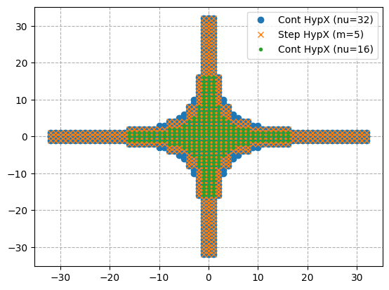
Figure 1. The step hyperbolic cross $Q_{m,{\bm{\gamma}},d}^{\alpha}$ for $m=5$ and $d=2$, and the continuous hyperbolic crosses $K^{\alpha}_{2^{m-(d-1)},{\bm{\gamma}},d}$ and $K^{\alpha}_{2^{m},{\bm{\gamma}},d}$.

3.6.1. Error analysis for weighted Wiener algebras

We may use Lemma 3.16 and reduce the error analysis in the case where we choose our index sets as step hyperbolic crosses to the one in Section 3.4.1, where we choose them as continuous hyperbolic crosses.

Theorem 3.19.

Let $\alpha>1,\delta\in(0,\alpha-1),\tau\in(0,\alpha-1-\delta]$ and assume that $g\in{\mathcal{A}}_{\alpha,{\bm{\gamma}},d}$. Let $L$ be a prime number, and let ${\mathcal{Z}}$ be a lattice point set of size $L$ satisfying (22). Then it holds for $m\in{\mathbb{N}}$

$$\left|\frac{1}{N}\sum_{n=1}^{N}c_{n}g({\bm{x}}_{n})-\frac{1}{L}\sum_{\ell=0}^{L-1}g({\bm{z}}_{\ell})\phi_{Q_{m,{\bm{\gamma}},d}^{\alpha}}({\bm{z}}_{\ell})\right|\leq\operatorname{err}_{1}(g,{\mathcal{C}})+\operatorname{err}_{2}(g,{\mathcal{C}})$$

$$\leq\left\|g\right\|_{{\mathcal{A}}_{\alpha,{\bm{\gamma}},d}}\left[\frac{1}{\sqrt{2^{m-d+1}}}+\frac{\sqrt{2^{m}}}{L^{\alpha-\frac{1}{2}-\delta-\tau}}c_{\alpha,{\bm{\gamma}},d}\zeta_{\delta,d}C_{{\bm{\gamma}},d}\left(\alpha-\frac{1}{2}-\delta,\tau\right)\right]\frac{1}{N}\sum_{n=1}^{N}\left|c_{n}\right|,$$

where $\operatorname{err}_{1}(g,{\mathcal{C}})$ and $\operatorname{err}_{2}(g,{\mathcal{C}})$ are defined as in (8) and (10), $c_{\alpha,{\bm{\gamma}},d}$ and $\zeta_{\delta,d}$ are as in (16), and $C_{{\bm{\gamma}},d}(\alpha,\tau)$ as in (22).

Proof.

We use again (8) and Lemma 3.1 to bound $\operatorname{err}_{1}(g,{\mathcal{C}})$. Hence, we need an estimate on $\sup_{{\bm{k}}\notin Q_{m,{\bm{\gamma}},d}^{\alpha}}1/\sqrt{r_{\alpha}({\bm{\gamma}},{\bm{k}})}$. Since $Q_{m,{\bm{\gamma}},d}^{\alpha}\supseteq K^{\alpha}_{2^{m-d+1},{\bm{\gamma}},d}$, see Lemma 3.16, we get

$$\sup_{{\bm{k}}\notin Q_{m,{\bm{\gamma}},d}^{\alpha}}\frac{1}{\sqrt{r_{\alpha}({\bm{\gamma}},{\bm{k}})}}\leq\sup_{{\bm{k}}\notin K^{\alpha}_{2^{m-d+1},{\bm{\gamma}},d}}\frac{1}{\sqrt{r_{\alpha}({\bm{\gamma}},{\bm{k}})}}\leq\frac{1}{\sqrt{2^{m-d+1}}},$$

which means

$$\operatorname{err}_{1}(g,{\mathcal{C}})\leq\frac{\left\|g\right\|_{{\mathcal{A}}_{\alpha,{\bm{\gamma}},d}}}{\sqrt{2^{m-d+1}}}\frac{1}{N}\sum_{n=1}^{N}\left|c_{n}\right|.$$

For $\operatorname{err}_{2}(g,{\mathcal{C}})$, we may apply Lemma 3.4 by estimating $\max_{{\bm{k}}\in Q_{m,{\bm{\gamma}},d}^{\alpha}}\sqrt{r_{\alpha}({\bm{\gamma}},{\bm{k}})}$. Since $Q_{m,{\bm{\gamma}},d}^{\alpha}\subseteq K^{\alpha}_{2^{m},{\bm{\gamma}},d}$, see Lemma 3.16, we get

$$\max_{{\bm{k}}\in Q_{m,{\bm{\gamma}},d}^{\alpha}}\sqrt{r_{\alpha}({\bm{\gamma}},{\bm{k}})}\leq\max_{{\bm{k}}\in K^{\alpha}_{2^{m},{\bm{\gamma}},d}}\sqrt{r_{\alpha}({\bm{\gamma}},{\bm{k}})}\leq\sqrt{2^{m}}.$$

With the estimate above and (22), we finally get

$$\operatorname{err}_{2}(g,{\mathcal{C}}) \leq\left\|g\phi_{Q_{m,{\bm{\gamma}},d}^{\alpha}}\right\|_{H_{\alpha-\frac{1}{2}-\delta,{\bm{\gamma}},d}}e(H_{\alpha-\frac{1}{2}-\delta,{\bm{\gamma}},d},{\mathcal{Z}})$$

$$\leq\left\|g\right\|_{{\mathcal{A}}_{\alpha,{\bm{\gamma}},d}}\frac{\sqrt{2^{m}}}{L^{\alpha-\frac{1}{2}-\delta-\tau}}c_{\alpha,{\bm{\gamma}},d}\zeta_{\delta,d}C_{{\bm{\gamma}},d}\left(\alpha-\frac{1}{2}-\delta,\tau\right)\frac{1}{N}\sum_{n=1}^{N}\left|c_{n}\right|.$$

The result now follows. ∎

Corollary 3.20.

Assume that the conditions of Theorem 3.19 hold, and let $\varepsilon>0$ be arbitrary. By choosing $\sigma=\sigma(\varepsilon)>0$ sufficiently small and the parameter $m$ as $m=\left(\alpha-\frac{1}{2}-\sigma\right)\log_{2}(L)+(d-1)/2$, we get the error bound

(37) $$\operatorname{err}_{1}(g,{\mathcal{C}})+\operatorname{err}_{2}(g,{\mathcal{C}})\lesssim L^{-\left(\alpha-\frac{1}{2}\right)/2+\varepsilon},$$

where the implicit constant is independent of $L$.

3.6.2. Error analysis for weighted Korobov spaces

We have shown in Lemma 3.16 how the step hyperbolic cross is related to the continuous one. Similarly as in the case of weighted Wiener algebras in Section 3.6.1, we may use Lemma 3.16 in the case of weighted Korobov spaces and play the error analysis for step hyperbolic crosses back to the one for hyperbolic crosses. Therefore, we may conclude that if we use the truncation to a step hyperbolic cross $Q_{m,{\bm{\gamma}},d}^{\alpha}$, with $g\in H_{\alpha,{\bm{\gamma}},d}$, then, we may choose $m$ as in Corollary 3.20 to get the same error bound as mentioned in Corollary 3.10.

3.6.3. Precomputation of compression weights

To facilitate a fast computation of the compression weights, we represent the step hyperbolic cross as a suitable disjoint union of rectangles

$$Q_{m,{\bm{\gamma}},d}^{\alpha}=\bigcup_{\begin{subarray}{c}{\bm{t}}\in{\mathbb{N}}_{0}^{d}\\ \left\|t\right\|_{1}=m\end{subarray}}\left\{{\bm{k}}\in{\mathbb{Z}}^{d}:r_{\alpha}(\gamma_{1},k_{1})\leq 2^{t_{1}}\,\wedge\,\left\lfloor 2^{t_{j}-1}\right\rfloor<r_{\alpha}(\gamma_{j},k_{j})\leq 2^{t_{j}}\quad\text{for}\quad j=2,\ldots,d\right\}.$$

When deriving the formula for $\phi_{Q_{m,{\bm{\gamma}},d}^{\alpha}}({\bm{z}}_{\ell})$ it will become apparent that treating the first coordinate differently from the others allows us to reduce the computation cost of the weights by reducing the number of factors under the product sign by one. In the above representation, we call the vectors ${\bm{t}}$ as shape vectors. For $j\in[d]$ and $t_{j}\in{\mathbb{N}}_{0}$, define

$$\tau^{\textup{low}}_{j}:=\left\lfloor\left(\gamma_{j}2^{t_{j}-1}\right)^{1/2\alpha}\right\rfloor\quad\text{and}\quad\tau^{\textup{up}}_{j}:=\left\lfloor\left(\gamma_{j}2^{t_{j}}\right)^{1/2\alpha}\right\rfloor.$$

Note that for $t_{j}=0$, we have $\tau^{\textup{low}}_{j}=0$, as well as $\tau^{\textup{up}}_{j}=0$ for $\gamma_{j}<1$, and $\tau^{\textup{up}}_{j}=1$ for $\gamma_{j}=1$. We can now express the compression weights as follows

(38) $$\phi_{Q_{m,{\bm{\gamma}},d}^{\alpha}}({\bm{z}}_{\ell})= \frac{1}{N}\sum_{n=1}^{N}c_{n}\sum_{{\bm{k}}\in Q_{m,{\bm{\gamma}},d}^{\alpha}}\omega_{{\bm{k}}}({\bm{x}}_{n}-{\bm{z}}_{\ell})$$

$$= \frac{1}{N}\sum_{n=1}^{N}c_{n}\sum_{\begin{subarray}{c}{\bm{t}}\in{\mathbb{N}}_{0}^{d},\\ \left\|t\right\|_{1}=m\end{subarray}}\left(\sum_{r_{\alpha}(\gamma_{1},k_{1})\leq 2^{t_{1}}}\exp(2\pi ik_{1}(x_{n,1}-z_{\ell,1}))\right)\times$$

$$\times\prod_{j=2}^{d}\sum_{\left\lfloor 2^{t_{j}-1}\right\rfloor<r_{\alpha}(\gamma_{j},k_{j})\leq 2^{t_{j}}}\exp(2\pi ik_{j}(x_{n,j}-z_{\ell,j}))$$

$$= \frac{1}{N}\sum_{n=1}^{N}c_{n}\sum_{\begin{subarray}{c}{\bm{t}}\in{\mathbb{N}}_{0}^{d},\\ \left\|t\right\|_{1}=m\end{subarray}}\left(\sum_{k_{1}=-\tau^{\textup{up}}_{1}}^{\tau^{\textup{up}}_{1}}\exp(2\pi ik_{1}(x_{n,1}-z_{\ell,1}))\right)\times$$

$$\times\prod_{j=2}^{d}\left(\sum_{k_{j}=-\tau^{\textup{up}}_{j}}^{\tau^{\textup{up}}_{j}}-\sum_{k_{j}=-\tau^{\textup{low}}_{j}}^{\tau^{\textup{low}}_{j}}\right)\exp(2\pi ik_{j}(x_{n,j}-z_{\ell,j}))$$

$$= \frac{1}{N}\sum_{n=1}^{N}c_{n}\sum_{\begin{subarray}{c}{\bm{t}}\in{\mathbb{N}}_{0}^{d},\\ \left\|t\right\|_{1}=m\end{subarray}}D_{\tau^{\textup{up}}_{1}}(x_{n,1}-z_{\ell,1})\prod_{j=2}^{d}\left(D_{\tau^{\textup{up}}_{j}}(x_{n,j}-z_{\ell,j})-D_{\tau^{\textup{low}}_{j}}(x_{n,j}-z_{\ell,j})\right),$$

where the last line follows from the definition of the Dirichlet kernel in (32).

For a given ${\bm{t}}$, the product above, whose factors are a single Dirichlet kernel and differences of Dirichlet kernels, can be computed in $O(d)$ operations. The set of shape vectors

(39) $$T(m,d):=\left\{{\bm{t}}\in{\mathbb{N}}_{0}^{d}:\left\|{\bm{t}}\right\|_{1}=m\right\}$$

has cardinality

$$|T(m,d)|=\binom{d-1+m}{d-1}\leq\min\left(\frac{(d-1+m)^{m}}{m!},\frac{(d-1+m)^{d-1}}{(d-1)!}\right).$$

Hence the total cost of computing the compression weights $\phi_{Q_{m,{\bm{\gamma}},d}^{\alpha}}({\bm{z}}_{\ell})$ for $\ell=0,\dots,L-1$ is of the order

$$O\left(\min\left(\frac{(d-1+m)^{m}}{m!},\frac{(d-1+m)^{d-1}}{(d-1)!}\right)NLd\right).$$

The alternative to the algorithm described above is to use the two-step procedure as in Algorithm 1, where we could use the fast approximate Fourier transform for the first step, mentioned in (23). This transform for the step hyperbolic cross is known as the nonequispaced sparse FFT (NSFFT), and depends on the representation involving union over high-dimensional rectangles (35), see [23, Section 4.2] and [14]. Nevertheless, the total cost would still be unfavorable, see the discussion after (33). Moreover, the NSFFT implementation is only available for $d=2,3$.

4. Comparison to data compression with digital nets

In this section, we want to compare our compression algorithms based on lattice point sets with the ones of Dick and Feischl that are based on digital $(t,m,d)$-nets, see [8]. In their error analysis of higher order digital nets, see [8, Sect. 4.2.2], they consider as function spaces Sobolev spaces $W_{2,\alpha,d}$, where the order $\alpha\geq 2$ is a natural number. More precisely, the multivariate Hilbert space $W_{2,\alpha,d}$, $\alpha\in{\mathbb{N}}$, is the $d$-fold tensor product of the univariate unanchored Sobolev space defined as

$$W_{2,\alpha,1}=\left\{g\in L^{2}([0,1]):\forall j\in[\alpha]:g^{(j)}\in L^{2}([0,1])\right\},$$

endowed with the norm

$$\left\|g\right\|_{W_{2,\alpha,1}}^{2}=\sum_{j=0}^{\alpha-1}\left|\int_{[0,1]}g^{(j)}(x){\,\mathrm{d}x}\right|^{2}+\int_{[0,1]}\left|g^{(\alpha)}(x)\right|^{2}{\,\mathrm{d}x}.$$

Note that for $g\in H_{\alpha,\gamma,1}$ the summands for $j=1,\ldots,\alpha-1$ vanish due to (Lebesgue’s version of) the fundamental theorem of calculus and the periodicity of $g,g^{\prime},\ldots,g^{(\alpha-2)}$. Hence, due to (15), the Korobov space $H_{\alpha,\gamma,1}$ is continuously embedded into $W_{2,\alpha,1}$, and for the choice $\gamma=1/(2\pi)^{2\alpha}$ the embedding constant (i.e., the operator norm of the identical embedding) is given by $1$. The same holds for the function spaces of $d$-variate functions $H_{\alpha,{\bm{\gamma}},d}$ and $W_{2,\alpha,d}$ if we choose

(40) $$\gamma_{1}=\gamma_{2}=\dots=\gamma_{d}=(2\pi)^{-2\alpha},$$

since these spaces are the $d$-fold Hilbert space tensor products of $H_{\alpha,\gamma,1}$ and $W_{2,\alpha,1}$, respectively. We will stick to this choice of (equal) weights and denote the corresponding Korobov space $H_{\alpha,{\bm{\gamma}},d}$ (admittedly, with some abuse of notation) by $H_{\alpha,d}$, and will suppress the reference to the weights ${\bm{\gamma}}$ also in other notation. Although $W_{2,\alpha,d}$ is a bit larger than $H_{\alpha,d}$, since it contains in addition certain non-periodic functions, we believe that these choices of function spaces allow essentially for a fair comparison of the data compression approaches based on lattice point sets and digital nets. Indeed, in many results for numerical integration and approximation the convergence rates on both type of spaces (“periodic and non-periodic Sobolev spaces”) are the same.

For the analysis of plain digital $(t,m,d)$-nets, Dick and Feischl considered Sobolev spaces $W_{1,2,d}$ of functions with dominating mixed smoothness of order $\alpha=2$, endowed with the norm

$$\left\|g\right\|_{W_{1,2,d}}:=\sum_{{\bm{u}}\subseteq[d]}\sum_{{\bm{v}}\subseteq{\bm{u}}}\int_{[0,1]^{{\bm{v}}}}\left|\int_{[0,1]^{d-\left|{\bm{v}}\right|}}\left(\prod_{j\in{\bm{v}}}\partial_{z_{j}}^{2}\prod_{j\in{\bm{u}}\setminus{\bm{v}}}\partial_{z_{j}}\right)g({\bm{z}})\,\mathrm{d}{\bm{z}}_{[d]\setminus{\bm{v}}}\right|\,\mathrm{d}{\bm{z}}_{\bm{v}},$$

where the inner integral is over all variables $z_{i}$, $i\in[d]\setminus{\bm{v}}$, and in the outer integral over all $z_{j}$, $j\in{\bm{v}}$, see [8, Sect. 4.2.1]. Since these spaces are larger than the ones we considered previously in this paper, they do not allow for a fair comparison. Indeed, our results for Wiener algebras or Korobov spaces provide a substantially higher convergence rate than the ones presented in [8, Thm. 11 & Cor. 12]. That is why we stick to the Hilbert space case and compare the results from [8, Sect. 4.2.2] with our results for Korobov spaces $H_{\alpha,d}$.

4.1. Comparison of errors

In order to have a similar notation for comparison of lattices with digital $(t,m,d)$-nets in base $b$, we set $L=b^{m}$. This implies $m\asymp\log(L)$. Assume that $g\in W_{2,\alpha,d}$ for some integer $\alpha\geq 2$. Let ${\mathcal{Z}}$ be an order $\alpha$ digital $(t,m,d)$-net in base $b$. Then, as shown in [8, Theorem 13], it holds for $m-t\geq\nu\in{\mathbb{N}}$

$$\operatorname{err}_{1}(g,{\mathcal{C}})+\operatorname{err}_{2}(g,{\mathcal{C}})\lesssim\left\|g\right\|_{W_{2,\alpha,d}}\left(\nu^{2d-1}b^{-\nu}+m^{\alpha d}b^{-\alpha(m-\nu)}\right)\frac{1}{N}\sum_{n=1}^{N}\left|c_{n}\right|.$$

(Note that the previous inequality differs slightly from [8, Theorem 13], since Dick and Feischl did not take into account the whole error term $\operatorname{err}_{1}(g,{\mathcal{C}})$ as defined in (8), but only the term $\|g-g_{K}\|_{\infty}$, instead, cf. [8, Formula (17)].) One may now choose $\nu=\lceil\frac{\alpha}{\alpha+1}m\rceil$ to balance the powers of $b$ in the error terms above to get

(41) $$\operatorname{err}_{1}(g,{\mathcal{C}})+\operatorname{err}_{2}(g,{\mathcal{C}})\lesssim m^{\alpha d}b^{-\alpha m/(\alpha+1)}\asymp L^{-\frac{\alpha}{\alpha+1}}\log(L)^{\alpha d},$$

as stated in [8, Remark 15].

Let $\alpha>1$ and assume that $g\in H_{\alpha,d}$. Let ${\mathcal{Z}}$ be a lattice point set of size $L$, where $L$ is a prime number. We denote the continuous hyperbolic cross based on equal weights as in (40) by $K_{\nu,d}^{\alpha}$. For an $\varepsilon>0$ that can be chosen arbitrarily small, we may select the parameters of our compression algorithm based on $L$ and $K_{\nu,d}^{\alpha}$ as in Corollary 3.10 to get the error bound

(42) $$\operatorname{err}_{1}(g,{\mathcal{C}})+\operatorname{err}_{2}(g,{\mathcal{C}})\lesssim L^{-\left(\frac{\alpha-1}{2}+\frac{1}{8\alpha}\right)+\varepsilon}\log(L)^{\frac{d-1}{2}},$$

where the implicit constant is independent of $L$.

We conclude that the compression algorithm based on lattices and continuous hyperbolic crosses offers a better bound on the convergence rate than the one based on digital nets for all integers $\alpha>2$. Note, in particular, that the guaranteed (polynomial) convergence rate of the error in (41) is $\frac{\alpha}{\alpha+1}$, which is strictly smaller than $1$ for all values of $\alpha$, while the convergence rate in (42) is strictly larger than $1$ for any integer $\alpha>2$, increasing essentially linearly in $\alpha$, and can be arbitrarily high for sufficiently smooth functions.

4.2. Comparison of precomputation cost

We now compare the cost of computing the compression weights for the two approaches. Let us again emphasize that this cost belongs to the “realm of precomputation”, since the weights can be used over and over again to evaluate the approximate error (3) for arbitrary parameters $\theta$. Recall from the previous section, that the optimal choice of $\nu\in{\mathbb{N}}$ for $(t,m,d)$-digital nets is $\left\lceil m\alpha/(\alpha+1)\right\rceil$ for $\alpha\geq 2$. The precomputation cost of evaluating the compression weights $W_{{\mathcal{X}},{\mathcal{Z}},\nu,\ell},W_{{\mathcal{X}},{\mathcal{Y}},{\mathcal{Z}},\nu,\ell}$ for $\ell=0,\dots,b^{m}-1$ using the algorithm described in [8, Algo 2,Algo 3,Lemma 4,Algo 6,Lemma 7] is of the order

(43) $$d^{2}mb^{m}N\asymp d^{2}NL\log(L),$$

see also [8, Theorem 8]. A modified version of the previous algorithm, for $\alpha\geq 2$, was described in [8, Lemma 5], in case we know an upper bound on the $t$-value for the digital net. In this approach, the number of operations are reduced by using additional storage of size $N$. Then the cost of computing the compression weights with this modified approach for $\nu=\left\lceil m\alpha/(\alpha+1)\right\rceil$ and $t\leq m/(\alpha+1)$ is of the order

(44) $$\binom{d-1+\nu}{d-1}Nb^{m/(\alpha+1)+d-1}\asymp\binom{d-1+\nu}{d-1}b^{d-1}NL^{1/(\alpha+1)},$$

where $m=\log_{b}(L)\in{\mathbb{N}}$, see [8, Lemma 5]. Let us again stress that we assume $L$ to be relatively small compared to $N$. That is why the second bound (44) is only preferable to (43), if the dimension $d$ is rather small in terms of $L$.

Looking at the three different variants of our lattice-based compression algorithm, we see that the minimal precomputation or “start up” cost is obtained if we consider the high-dimensional rectangle, i.e., $K=R^{\alpha}_{\nu,d}$. Here, we have a cost of $O(LNd)$, irrespective of the choice of $\nu$. This is due to the “Dirichlet kernel trick”: If we sum up trigonometric monomials $\omega_{\bm{k}}$, all evaluated in the same point ${\bm{x}}$, with frequency vectors ${\bm{k}}$ from a $d$-dimensional rectangle $R$, then the resulting sum can be reduced to a $d$-fold product of Dirichlet kernels, regardless of the size of $R$, cf. Section 3.5.3. Recall that the error bounds we obtained for rectangles are worse than the ones we derived for hyperbolic crosses, which is why the former approach is, in general, less attractive. Nevertheless, for $\alpha$ large enough (i.e., essentially a bit larger than the dimension $d$), the convergence rate of the errors from Corollary 3.15 for the rectangle setting is higher than the one in (41) obtained in [8] with the help of digital $(t,m,d)$-nets. In that regime the rectangle approach has a better error bound as well as a preferable cost bound (in particular, with respect to the dimension dependence) than the approach based on digital nets from [8].

The lattice-based algorithm using the truncation to a step hyperbolic cross, $K=Q^{\alpha}_{\ell,d}$, exploits that $Q^{\alpha}_{\ell,d}$ is a composition of rectangles. Hence, the “Dirichlet kernel trick” can be used again to get a fast computation of the corresponding compression weights, see Section 3.6.3, which results in a cost of order

$$\binom{d-1+\ell}{d-1}NLd,\quad\text{ where }\ell:=\left\lceil\left(\alpha-\frac{1}{2}-\sigma\right)\log_{2}(L)+\frac{d-1}{2}\right\rceil,$$

and $\sigma>0$ can be chosen sufficiently small. The parameter $\ell$ is chosen according to Corollary 3.20.

The cost of computing the compression weights using Algorithm 1, for $\nu\asymp L^{\alpha-1/2-\sigma(\varepsilon)}$ for the continuous hyperbolic cross $K_{\nu,d}^{\alpha}$, chosen according to Corollary 3.8 and Corollary 3.10, along with the estimates from (26) and (30), is of the order

$$dNL^{\frac{1}{2}-\frac{1}{4\alpha}-\varepsilon}\left(1+2\zeta(1+2\alpha\varepsilon)\right)^{d},$$

where $\varepsilon>0$ can be chosen arbitrarily small, and the hidden constants are independent of $N$ and $L$, see Section 3.4. Essentially, Algorithm 1 could also be used in combination with the step-hyperbolic cross, and this would cost at most as much as combining it with the continuous hyperbolic cross, since we have shown $Q_{m,{\bm{\gamma}},d}^{\alpha}\subseteq K_{\nu,{\bm{\gamma}},d}^{\alpha}$ for $\nu=2^{m}$. This approach would improve if there is a faster method at hand to solve the NDFT formulation, see (23).

As is indicated from the analysis for the high-dimensional rectangle, we may get even better cost estimates if we trade for a weaker error bound. To illustrate this point, let us discuss one example for $\alpha\geq 2$. For any $\epsilon>0$, there exist $\sigma=\sigma(\epsilon)>0$ and $\varepsilon=\varepsilon(\epsilon)$ such that we obtain for the continuous hyperbolic cross $K=K^{\alpha}_{\nu,d}$ with $\nu\asymp L^{\frac{4\alpha^{2}}{(\alpha+1)(2\alpha-1)}-\sigma}$ from Theorem 3.9 the error bound

$$\operatorname{err}_{1}(g,{\mathcal{C}})+\operatorname{err}_{2}(g,{\mathcal{C}})\lesssim\left\|g\right\|_{H_{\alpha,d}}L^{-\frac{\alpha}{\alpha+1}+\epsilon}\log(L)^{\frac{d-1}{2}},$$

and the cost of precomputing the compression weights is of the order

$$dNL^{\frac{1}{(\alpha+1)(1-1/2\alpha)}+\epsilon}\left(1+\pi^{-1-2\alpha\varepsilon}\zeta(1+2\alpha\varepsilon)\right)^{d}.$$

Note that these results are very close to the ones obtained in [8] for digital nets.

Acknowledgment

The authors would like to thank Josef Dick, Michael Feischl, Stefan Kunis, and Dirk Nuyens for valuable discussions.

Part of the work on this paper was done while all three authors attended the Dagstuhl workshop 23351, “Algorithms and Complexity for Continuous Problems". The authors thank the Leibniz Center for Informatics, Schloss Dagstuhl, and its staff for their support and their hospitality.

The first and the third author would also like to thank the Isaac Newton Institute for Mathematical Sciences (INI), Cambridge, for support and hospitality during the programme “Multivariate approximation, discretization, and sampling recovery”, where work on this paper was undertaken. This work was supported by EPSRC grant EP/R014604/1.

References

[1]Claude J.. Bélisle“Convergence Theorems for a Class of Simulated Annealing Algorithms on ”In Journal of Applied Probability29.4Applied Probability Trust, 1992, pp. 885–895DOI: 10.2307/3214721
[2]Frank F. Bonsall and John Duncan“Complete Normed Algebras”In Springer Berlin Heidelberg eBooks, 1973DOI: 10.1007/978-3-642-65669-9
[3]O. Bousquet et al.“No random, no cry” Preprint, arXiv: 1706.03200v1, 2017
[4]C.. Broyden“The Convergence of a Class of Double-rank Minimization Algorithms 1. General Considerations”In IMA Journal of Applied Mathematics6.1, 1970, pp. 76–90DOI: 10.1093/imamat/6.1.76
[5]James W. Cooley and John W. Tukey“An algorithm for the machine calculation of complex Fourier series”In Mathematics of Computation19.90, 1965, pp. 297–301DOI: 10.1090/S0025-5718-1965-0178586-1
[6]Ronald Cools, Frances Y. Kuo and Dirk Nuyens“Constructing lattice rules based on weighted degree of exactness and worst case error”In Computing87.1, 2010, pp. 63–89DOI: 10.1007/s00607-009-0076-1
[7]J. Dick and F. Pillichshammer“Digital Nets and Sequences”Cambridge: Cambridge University Press, 2010
[8]Josef Dick and Michael Feischl“A quasi-Monte Carlo data compression algorithm for machine learning”In Journal of Complexity67, 2021, pp. 101587DOI: 10.1016/j.jco.2021.101587
[9]Josef Dick, Peter Kritzer, Gunther Leobacher and Friedrich Pillichshammer“A reduced fast component-by-component construction of lattice points for integration in weighted spaces with fast decreasing weights”In Journal of Computational and Applied Mathematics276, 2015, pp. 1–15DOI: 10.1016/j.cam.2014.08.017
[10]Josef Dick, Peter Kritzer and Friedrich Pillichshammer“Lattice Rules: Numerical Integration, Approximation, and Discrepancy” 58, Springer Series in Computational MathematicsCham: Springer International Publishing, 2022DOI: 10.1007/978-3-031-09951-9
[11]Dinh Dũng, Vladimir Temlyakov and Tino Ullrich“Hyperbolic Cross Approximation”, Advanced Courses in Mathematics - CRM BarcelonaSpringer International Publishing, 2018URL: https://books.google.de/books?id=xQJ2DwAAQBAJ
[12]Adrian Ebert and Peter Kritzer“Constructing lattice points for numerical integration by a reduced fast successive coordinate search algorithm”In Journal of Computational and Applied Mathematics351, 2019, pp. 77–100DOI: 10.1016/j.cam.2018.10.046
[13]Adrian Ebert, Hernan Leövey and Dirk Nuyens“Successive Coordinate Search and Component-by-Component Construction of Rank-1 Lattice Rules”In Monte Carlo and Quasi-Monte Carlo Methods 2016Cham: Springer International Publishing, 2018, pp. 197–215DOI: 10.1007/978-3-319-91436-7_10
[14]Markus Fenn, Stefan Kunis and Daniel Potts“Fast evaluation of trigonometric polynomials from hyperbolic crosses”In Numerical Algorithms41.4, 2006, pp. 339–352DOI: 10.1007/s11075-006-9017-7
[15]R. Fletcher“A new approach to variable metric algorithms”In The Computer Journal13.3, 1970, pp. 317–322DOI: 10.1093/comjnl/13.3.317
[16]Jerome Friedman, Trevor Hastie and Robert Tibshirani“Regularization Paths for Generalized Linear Models via Coordinate Descent”In Journal of Statistical Software33.1, 2010DOI: 10.18637/jss.v033.i01
[17]Donald Goldfarb“A family of variable-metric methods derived by variational means”In Mathematics of Computation24.109, 1970, pp. 23–26DOI: 10.1090/S0025-5718-1970-0258249-6
[18]Arthur E. Hoerl and Robert W. Kennard“Ridge Regression: Applications to Nonorthogonal Problems”In Technometrics12.1, 1970, pp. 69–82DOI: 10.1080/00401706.1970.10488635
[19]Arthur E. Hoerl and Robert W. Kennard“Ridge Regression: Biased Estimation for Nonorthogonal Problems”In Technometrics12.1, 1970, pp. 55–67DOI: 10.1080/00401706.1970.10488634
[20]Lutz Kämmerer“Reconstructing Hyperbolic Cross Trigonometric Polynomials by Sampling along Rank-1 Lattices”In SIAM Journal on Numerical Analysis51.5, 2013, pp. 2773–2796DOI: 10.1137/120871183
[21]Lutz Kämmerer, Stefan Kunis and Daniel Potts“Interpolation lattices for hyperbolic cross trigonometric polynomials”In Journal of Complexity28.1, 2012, pp. 76–92DOI: 10.1016/j.jco.2011.05.002
[22]Lutz Kämmerer, Daniel Potts and Toni Volkmer“Approximation of multivariate periodic functions by trigonometric polynomials based on rank-1 lattice sampling”In Journal of Complexity31.4, 2015, pp. 543–576DOI: https://doi.org/10.1016/j.jco.2015.02.004
[23]Jens Keiner, Stefan Kunis and Daniel Potts“Using NFFT 3—A Software Library for Various Nonequispaced Fast Fourier Transforms”In ACM Trans. Math. Softw.36.4New York, NY, USA: Association for Computing Machinery, 2009DOI: 10.1145/1555386.1555388
[24]Yurii Kolomoitsev, Tetiana Lomako and Sergey Tikhonov“Sparse Grid Approximation in Weighted Wiener Spaces”In Journal of Fourier Analysis and Applications29.2, 2023, pp. 19DOI: 10.1007/s00041-023-09994-2
[25]Frances Y. Kuo“Component-by-component constructions achieve the optimal rate of convergence for multivariate integration in weighted Korobov and Sobolev spaces”In Journal of Complexity19.3, Oberwolfach Special Issue, 2003, pp. 301–320DOI: 10.1016/S0885-064X(03)00006-2
[26]Frances Y. Kuo, Ian H. Sloan and Henryk Woźniakowski“Lattice Rules for Multivariate Approximation in the Worst Case Setting”In Monte Carlo and Quasi-Monte Carlo Methods 2004Berlin, Heidelberg: Springer, 2006, pp. 289–330
[27]Alan Miller“Subset Selection in Regression”New York: ChapmanHall/CRC, 2002DOI: 10.1201/9781420035933
[28]Balas K. Natarajan“Sparse Approximate Solutions to Linear Systems”In SIAM Journal on Computing24.2Society for IndustrialApplied Mathematics, 1995, pp. 227–234DOI: 10.1137/S0097539792240406
[29]John A. Nelder and Roger Mead“A Simplex Method for Function Minimization”In The Computer Journal7.4, 1965, pp. 308–313DOI: 10.1093/comjnl/7.4.308
[30]H. Niederreiter“Point sets and sequences with small discrepancy”In Monatsh. Math.104, 1987, pp. 273–337
[31]Erich Novak, Ian H. Sloan and Henryk Woźniakowski“Tractability of Approximation for Weighted Korobov Spaces on Classical and Quantum Computers”In Foundations of Computational Mathematics, 2004, pp. 121–156DOI: 10.1007/s10208-002-0074-6
[32]Erich Novak and Henryk Woźniakowski“Tractability of Multivariate Problems. Vol. 1: Linear Information”, EMS Tracts in MathematicsZürich: European Mathematical Society (EMS), 2008
[33]Dirk Nuyens and Ronald Cools“Fast algorithms for component-by-component construction of rank-1 lattice rules in shift-invariant reproducing kernel Hilbert spaces”In Mathematics of Computation75American Mathematical Society (AMS), 2006, pp. 903–920DOI: 10.1090/S0025-5718-06-01785-6
[34]Gerlind Plonka, Daniel Potts, Gabriele Steidl and Manfred Tasche“Numerical Fourier Analysis”, Applied and Numerical Harmonic AnalysisCham: Springer International Publishing, 2018DOI: 10.1007/978-3-030-04306-3
[35]D. Potts and M. Schmischke“Approximation of high-dimensional periodic functions with Fourier-based methods”In SIAM Journal on Numerical Analysis59, 2021, pp. 2393–2429
[36]Daniel Potts and Michael Schmischke“Interpretable Approximation of High-Dimensional Data” Publisher: Society for Industrial and Applied MathematicsIn SIAM Journal on Mathematics of Data Science3.4, 2021, pp. 1301–1323DOI: 10.1137/21M1407707
[37]Daniel Potts and Michael Schmischke“Interpretable Transformed ANOVA Approximation on the Example of the Prevention of Forest Fires”In Frontiers in Applied Mathematics and Statistics8, 2022URL: https://www.frontiersin.org/articles/10.3389/fams.2022.795250
[38]D.. Shanno“Conditioning of quasi-Newton methods for function minimization”In Mathematics of Computation24.111, 1970, pp. 647–656DOI: 10.1090/S0025-5718-1970-0274029-X
[39]Ian H. Sloan and Andrew V. Reztsov“Component-by-component construction of good lattice rules”In Mathematics of Computation71, 2002, pp. 263–273URL: https://api.semanticscholar.org/CorpusID:7003618
[40]Ian H. Sloan and Henryk Woźniakowski“When Are Quasi-Monte Carlo Algorithms Efficient for High Dimensional Integrals?”In Journal of Complexity14.1, 1998, pp. 1–33DOI: 10.1006/jcom.1997.0463
[42]Robert Tibshirani“Regression Shrinkage and Selection via the Lasso”In Journal of the Royal Statistical Society. Series B (Methodological)58.1Royal Statistical Society, Wiley, 1996, pp. 267–288URL: https://www.jstor.org/stable/2346178