Cleaning WASP-33 b transits from the host star photometric variability: analysis of TESS data from two sectors

Abstract

Based on TESS observations of a $\delta$ Scuti variable WASP-33 obtained in 2019 and 2022, we thoroughly investigate the power spectrum of this target photometric flux and construct a statistically exhaustive model for its variability. This model contains $30$ robustly justified harmonics detected in the both TESS sectors simultaneously, $13$ less robust harmonics detected in a single TESS sector, a red noise and a quasiperiodic noise terms. This allowed us to greatly improve the accuracy of the exoplanet WASP-33 b transit timings, reducing the TTV residuals r.m.s. drastically, by a factor of $3.5$, from $63$ s to $18$ s. Finally, our analysis does not confirm existence of a detectable orbital phase variation claimed by von Essen et al. (2020) based on WASP-33 TESS photometry of 2019.

1 Introduction

WASP-33 (HD 15082) is a bright 8.14 mag fast-rotating star with $v\sin i\sim 90$ km/s, located in Andromeda. Its the only known exoplanet WASP-33 b was detected by SuperWASP (Herrero et al., 2011). Its orbital period is estimated by $P_{b}=(1.219867\pm 4.2\cdot 10^{-5})$ d (von Essen et al., 2020), mass by $M_{b}=(2.10\pm 0.14)$ $M_{\rm Jup}$, and radius by $r_{b}=(1.59\pm 0.07)$ $R_{\rm Jup}$ (Chakrabarty & Sengupta, 2019). It is remarkable that this exoplanet was the first one ever known to orbit a $\delta$ Scuti variable.

The variability of the prototype star itself, $\delta$ Scuti, was discovered in the beginning of XX century (Campbell & Wright, 1900), and then it was confirmed by spectral and photometric observations (Colacevich, 1935; Fath, 1935). Furthermore, Eggen (1956) combined this and a few similar stars together in a standalone class of variables, and so the $\delta$ Scuti type of variable stars appeared.

These variables are pulsating stars belonging to spectral classes A0-F5 III-IV, located in the instability strip of the HR diagram (Baglin et al., 1973; Breger & Stockenhuber, 1983). Their $m_{V}$ variation amplitudes range from $0.003$ to $0.9$ (typically a few hundreds) and periods from $0.01$ d to $0.2$ d. Most of the $\delta$ Scuti stars belong to type I population (Breger, 1979), with a typical mass of $\sim 2$ $M_{\odot}$ (Milligan & Carson, 1992). The power spectrum of $\delta$ Scuti variables may reveal tens of periods (Breger et al., 1999) ranging from hours to minutes. Such stars often exhibit significant changes in the form of their lightcurve, in their variability period and amplitude. Radial as well as non-radial pulsations can be observed. Nonradial pulsations indicate concurrent inward and outward surface moves, contrary to radial ones which reflect expansions and contractions of the star as a whole. A key role in the pulsation generating mechanism belongs to helium which is highly abundant in the atmosphere of these stars. When helium is heated and ionized it gains opacity, causing the star brightness be at minimum. However, the radiation absorbed makes helium to heat further and expand, causing its recombination, transparency increase and the star brightness to reach the maximum. Then helium starts to cool down and the cycle restarts again (Cox, 1963).

Large amount of data regarding $\delta$ Scuti variables were brought by (i) OGLE and MACHO surveys which detected about $3000$ such variables in the Large Magellanic Cloud (Poleski et al., 2010; Garg et al., 2010), (ii) Kepler spacecraft (Borucki et al., 2010) that found about $750$ candidate variables of this type, and (iii) TESS (Transiting Exoplanet Survey Satellite) space mission, for example (Antoci et al., 2019) analyzed a sample of $117$ variables belonging to $\delta$ Scuti and $\gamma$ Doradus class.

The intrinsic variability of WASP-33 represents an obvious nuisance factor for analysing its exoplanet b transit lightcurves. The effect of this variability on the estimated planetary orbital parameters was previously investigated using out-of-transit observations from ground-based telescopes located in Germany and Spain (von Essen et al., 2014). Their investigation of the WASP-33 pulsations power spectrum revealed eight significant frequencies. It was concluded that cleaning the transit lightcurves from stellar pulsations practically does not affect estimated planetary parameters, but their uncertainties get decreased. Besides, von Essen et al. (2014) noticed that WASP-33 pulsations phases change over time. In a later analysis of TESS photometry of 2019, von Essen et al. (2020) claimed the detection of $29$ pulsation frequencies. In addition to the power spectrum analysis, they also reported statistically significant detection of WASP-33 b secondary eclipse and of the orbital phase curve variation (period of $P_{b}$, amplitude of $(100.4\pm 13.1)$ ppm). Also, they took into account the “ellipsoidal variation” that appears because of planetary gravitational effect on the star shape (period of $P_{b}/2$, theoretically predicted amplitude of $27.4$ ppm).

A more recent analysis of WASP-33 variability was performed using data from TESS (Kálmán et al., 2022). They investigated the Fourier spectrum of stellar oscillations reconstructed with TLCM (Transit and Light Curve Modeller, Csizmadia et al. 2023). This spectrum revealed three peaks with $S/N>8$ that were close to a commensurability with the planetary orbital period ($1:3$, $1:12$, and $1:25$). It was argued that the distribution of $17$ frequencies with the largest amplitudes tend to shift right from these subharmonics. As Kálmán et al. (2022) noticed, this effect can be caused by the tidal perturbations from the planet.

Our primary goal here is to analyse WASP-33 pulsations spectrum based on the up-to-date TESS data (observations of 2019 and 2022), and to investigate whether (and how much) this can help us to improve the transit timings accuracy for the exoplanet WASP-33 b.

2 TESS photometry of WASP-33

TESS observed WASP-33 in sector 18 (Nov 2019) and sector 58 (Nov 2022), lasting about $1$ month each. In the DVT data downloaded from the MAST (Mikulski Archive for Space Telescopes) we found $14796$ and $18951$ photometric measurements for these two sectors, respectively. We identified $17$ transits in sector 18 and $21$ transits in sector 58, and for each transit we extracted a $\pm 4$ h piece of the lightcurve about the predicted midtransit epoch. This subset formed our “in-transit” dataset (ITD). The “out-of-transit” dataset (OTD) included all observations located at least $\pm 2$ h away from the centers of transits and secondary eclipses. Notice that ITD and OTD slightly overlap.

In this work we will deal mainly with the OTD, since we aim to construct a model for the intrinsic star variability. The sector 18 portion of the OTD will be hereafter refered to as TESS₁₈, and it contains $10684$ datapoints. The sector 58 OTD portion (TESS₅₈) contains $13625$ datapoints. ITD contains $8914$ datapoints in total, with $\sim 200$ observations per transit.

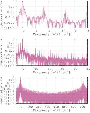
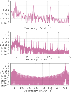
Figure 1: Spectral window of the TESS₁₈ (left) and TESS₅₈ (right) data, for three frequency ranges (from top to bottom). The (quasi-)Nyquist alias peak at $2f_{\rm Ny}=720$ d^-1 is seen in the bottom panels.

TESS data look close to being even with a constant timestep of $\Delta t=2$ min. However, this is not strictly fulfilled even within just a single sector, because in the middle of each sector there was a gap, after which the $2$ min grid pattern got shifted. Also, the OTD set contains holes in place of transits and secondary eclipses. But nevertheless the spectral window functions of TESS_18,58 data suggest that these data can be treated as nearly even, in particular there is a classic aliasing pattern suggesting the existence of a “quasi-Nyquist“ frequency $f_{\rm Ny}=1/(2\Delta t)=360$ d^-1 (see Fig. 1).

3 Building the statistically exhaustive model of WASP-33 variability

Here our goal is to construct a statistically “exhaustive” WASP-33 model that represents its OTD so that the residuals do not contain statistically significant periodic (or quasiperiodic) variations. In this attempt we aimed to apply a periodogram-based approach somewhat reminiscent of the CLEANest algorithm by Foster (1995). Namely, we represent the photometric variation as a sum of sinusoidal harmonics:

$$\mu_{n}(t)=A_{0}+\sum_{k=1}^{n}A_{k}\cos\left(2\pi f_{k}(t-T_{0})+\varphi_{k}\right),$$ (1)

where $A_{k}$, $\varphi_{k}$, and $f_{k}=1/P_{k}$ are free parameters.

However, if the model (1) was used in the white noise (WN hereafter) treatment then we would likely need hundreds of harmonics to represent the OTD exhaustively. After extraction of some initial (the most significant) harmonics, the residual periodogram did not reveal a single clearly dominating peak, looking more similar to a spectrum of non-white (banded) noise.

Alone such an observation is not yet decisive to claim that the data physically involve non-white noise (NWN hereafter). Two alternative models “a lot of harmonics + WN” and “fewer harmonics + NWN” may appear formally indistinguishable, i.e. statistically equivalent in how well they describe the data. But even in this case the NWN model may offer a great reduction in the number of model components (and parameters), so we can profit from a mathematically more simple $\mu$.

To take the NWN into account, we adopted an approach of Gaussian process (GP) fitting, introduced in (Baluev, 2011). In this approach we should define a model for the NWN correlation function, which we now set to:

$$k_{n^{\prime}}(\Delta t_{ij}) =\left(\sigma_{{\rm TESS},i}^{2}+\sigma_{0}^{2}\right)\delta_{ij}+\sum_{k=1}^{n^{\prime}}\sigma_{k}^{2}{\rm e}^{-\frac{|\Delta t_{ij}|}{\tau_{k}}}\cos 2\pi f^{\prime}_{k}\Delta t_{ij},$$

$$\phantom{=}\Delta t_{ij}=t_{i}-t_{j},$$ (2)

where $\sigma_{{\rm TESS},i}$ is TESS-provided photometric uncertainty at $t_{i}$, $\delta_{ij}$ is Kronecker delta, while $\sigma_{k}$, $\tau_{k}$, and $f^{\prime}_{k}=1/P^{\prime}_{k}$ are free parameters. This model involves the WN portion ($\sigma_{0}$) and $n^{\prime}$ independent quasiperiodic components (purely NWN part). By a visual look at the periodograms (e.g. see Fig. 2 discussed below) we noticed three possible spectrum bands that are concentrated near the frequencies $f^{\prime}_{1}\simeq 0$, $f^{\prime}_{2}\simeq 10$ d^-1, and $f^{\prime}_{3}\simeq 20$ d^-1. We set these frequencies as starting values for the GP fitting, thus assuming $n^{\prime}=3$.

Then we run a sequential periodogram algorithm according to the following scheme. We started from $k_{3}$ as specified above, and from $\mu_{2}$ involving two harmonics with fixed frequencies as per von Essen et al. (2020): $f_{1}=P_{b}$ (orbital phase variation) and $f_{2}=P_{b}/2$ (ellipsoidal variation). After that the model (1) can be built up iteratively by adding harmonics that refer to the tallest peak in the subsequent residual periodogram. These periodograms must take the NWN into account via (2). For that we used the formalism of the likelihood-ratio periodogram (LRP) introduced by Baluev (2009, 2013b) and implemented in the PlanetPack software (Baluev, 2013a, 2018). The LRP considers two rival models of the data, a base one ($\mu_{n}$ on $n$th iteration) and an alternative one involving an extra sinusoid (i.e. $\mu_{n+1}$). The likelihood ratio statistic is then computed for these models and its logarithm is plotted against the frequency of the last added sinusoid. Such a graph represents our LRP that generalises the classic Lomb (1976) – Scargle (1982) periodogram. The LRP can be computed for the classic WN case as well as for the NWN model (2), by defining the likelihood function appropriately. After each iteration all free parameters of so far detected harmonics are refined by refitting with the new model $\mu$.

Very importantly, the spectral window in Fig. 1 does not demonstrate large side peaks (in the Nyquist range at least). The height of the tallest side peak is $\simeq 0.1$. Therefore, the aliasing appears insignificant in our task, and we may safely assume that the maximum periodogram peak corresponds to the true (rather than alias) frequency. This makes all the analysis easier, for example it is unnecessary to care about the order in which the harmonics are extracted (which could be important otherwise).

However, dealing with NWN periodograms implies numerous NWN model refitting, which is computationally demanding. The likelihood function involves operations on very large covariance matrices ($\sim 10^{4}\times 10^{4}$), rendering the LRP computation too slow for being accomplished in full. But we tried to bypass this limitation using the following approach. On each iteration we computed, at first, the fast WN-only version of the LRP, and determined its $256$ tallest peaks. Then for each of these peaks we run an NWN maximum-likelihood fitting, starting it from the associated WN best fit. This allowed us to compute heights of these same peaks in the NWN treatment, and then to select the tallest one among them.

Such an approach is potentially vulnerable because it may, in theory, miss the actual best-significance harmonic. Even $256$ peaks that appeared tallest with the WN model do not necessarily contain the one that should appear tallest in the NWN case. However, the probability of such a condition decreases when the number of peaks being inspected grows, so the validity of the results can be tested by a probe increase of that number (in the end of iterations sequence).

We launched our harmonics detection iterations assuming the frequency range from $f=0$ to $f=50$ d^-1, which is a priori reasonable for $\delta$ Scuti stars, and also contained all apparently noticeable periodogram power. As we specified above, the NWN model (2) was initially set to have $n^{\prime}=3$ terms, but somewhere in the middle of the sequence the third NWN term (with $f^{\prime}\simeq 20$ d^-1) appeared, basically, decomposed into harmonics. We started to obtain various degeneracy issues regarding this term, for example it was trying to either model just a single sinusoid ($\tau\to 0$), or to mimic a portion of the white noise ($\tau\to\infty$), or to model a portion of another NWN term. When this behaviour started, we manually removed this third term from the NWN model, and continued the sequence further with $k_{2}(\Delta t)$ instead of $k_{3}(\Delta t)$. Finally, when no significant harmonics left (in the NWN treatment), we reprocessed the last iteration inspecting $1024$ tallest peaks instead of just $256$, and in the entire Nyquist range (max frequency of $360$ d^-1 instead of $50$ d^-1). This did not result in detection of additional harmonics, ensuring that we did not miss any.

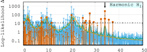
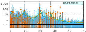
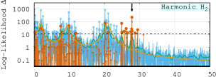
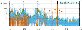
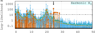
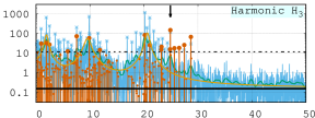
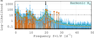
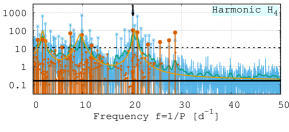
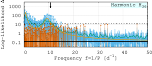
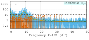
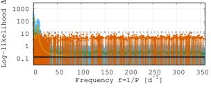
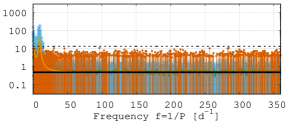
Figure 2: Periodogram analysis and extraction of the harmonics.

This algorithm was applied to TESS₁₈ and TESS₅₈ data separately, and gave similar results. Some graphs illustrating the initial and final iterations are shown in Fig. 2. Each panel demonstrates the WN periodograms (raw as well as smoothed one), the theoretic power spectrum of the current best fitting NWN model based on (2), and the set of NWN peaks that were dealt with on this iteration. On the last iteration, when we inspected $1024$ peaks, those peaks are covering the entire Nyquist range without significant holes or blind segments, so it is very unlikely that some statistically significant harmonics escaped our analysis. Please also notice remarkable similarity between our fitted NWN power spectrum and the smoothed WN periodogram.

Some explanation should also be given regarding how we computed the statistical significance of periodogram peaks in the NWN treatment. As explained in (Baluev, 2009), for the WN type of the LRP we may use the following approximation of the False Alarm Probability (FAP) from (Baluev, 2008):

$${\rm FAP}(z)\stackrel{{\scriptstyle z\gg 1}}{{\simeq}}W{\rm e}^{-z}\sqrt{z},\quad W=(f_{\max}-f_{\min})T_{\rm eff},$$ (3)

where $z$ is the height of the tallest peak, and $T_{\rm eff}$ is an effective time span proportional to the sample variance of the timings $t_{i}$. As argued (without proofs) in (Baluev, 2015), the approximate formula (3) remains applicable for NWN models as well, but with $T_{\rm eff}$ somewhat differently determined. Delisle et al. (2020) developed this study further, partly confirming this conclusion and providing a more general definition for $T_{\rm eff}$. However, in our task it appeared that $T_{\rm eff}$ always remains practically identical, regardless of the noise model or which approximation to adopt. We obtained $T_{\rm eff}$ about $24$ d for TESS₁₈ and about $28$ d for TESS₅₈.

In this study we aimed to obtain a more accurate final model of the WASP-33 variability, possibly even by the cost of larger probability of false positive harmonics. So we adopted a relatively mild FAP threshold of $5\%$ (the iterations continued until the right hand side of (3) exceeded $0.05$).

Table 1: Estimated harmonics parameters.

		TESS18 ($T_{0}=2458800$)			TESS58 ($T_{0}=2459895$)
IDs		$P$ [d]	$A$ [ppm]	$\varphi$ [∘]	$P$ [d]	$A$ [ppm]	$\varphi$ [∘]
$H_{1}$					$0.0213065(17)$	$41.7(8.0)$	$328(11)$
$H_{2}$	$F_{10}$	$0.02930411(56)$	$228.3(6.8)$	$297.9(1.8)$	$0.02930358(45)$	$312.5(8.3)$	$279.2(1.5)$
$H_{3}$	$F_{28}$	$0.0328267(44)$	$38.0(7.0)$	$306(11)$
$H_{4}$	$F_{26}$	$0.0331895(39)$	$44.5(7.1)$	$37.1(9.8)$	$0.0331986(43)$	$42.4(8.5)$	$155(12)$
$H_{5}$	$F_{22}$	$0.0348597(28)$	$69.6(7.2)$	$206.2(6.4)$	$0.0348553(16)$	$130.6(8.7)$	$186.8(3.8)$
$H_{6}$	$F_{8}$	$0.03597781(78)$	$267.3(7.3)$	$317.9(1.7)$	$0.03597797(38)$	$580.6(8.7)$	$93.27(87)$
$H_{7}$	$F_{18}$	$0.0364189(26)$	$84.0(7.3)$	$180.1(5.4)$	$0.0364150(26)$	$86.0(8.7)$	$315.9(5.9)$
$H_{8}$					$0.0373459(57)$	$42.3(8.8)$	$154(12)$
$H_{9}$	$F_{14}$	$0.0390044(23)$	$111.5(7.5)$	$198.8(4.2)$	$0.0390015(30)$	$87.9(8.9)$	$214.6(5.9)$
$H_{10}$	$F_{9}$	$0.0401869(11)$	$253.0(7.8)$	$11.5(1.9)$	$0.0401856(11)$	$258.3(9.1)$	$118.1(2.1)$
$H_{11}$		$0.0406911(67)$	$43.5(8.0)$	$9(11)$
$H_{12}$	$F_{16}$	$0.0430933(35)$	$102.1(8.2)$	$258.8(5.1)$	$0.0430910(30)$	$114.8(9.4)$	$55.1(4.8)$
$H_{13}$	$F_{27}$	$0.0440461(85)$	$41.3(8.7)$	$121(13)$	$0.0440554(71)$	$51(10)$	$221(11)$
$H_{14}$	$F_{20}$	$0.0451501(44)$	$90.3(8.5)$	$224.4(6.0)$	$0.0451491(44)$	$91.3(9.9)$	$245.1(6.1)$
$H_{15}$		$0.0454574(96)$	$40.6(8.6)$	$103(13)$
$H_{16}$		$0.0457087(92)$	$43.5(8.7)$	$60(12)$	$0.0457113(72)$	$56.2(9.8)$	$194(10)$
$H_{17}$	$F_{19}$	$0.0460159(54)$	$76.8(8.8)$	$261.9(7.0)$	$0.0460004(57)$	$72.1(9.8)$	$73.5(7.8)$
$H_{18}$		$0.0465026(83)$	$53.0(8.8)$	$296(10)$
$H_{19}$	$F_{24}$	$0.0469927(71)$	$61.5(8.8)$	$164.0(8.7)$	$0.0469969(49)$	$85.6(9.7)$	$268.1(6.5)$
$H_{20}$	$F_{4}$	$0.04747567(95)$	$617(11)$	$335.46(96)$	$0.04747626(78)$	$618(11)$	$161.2(1.0)$
$H_{21}$	$F_{11}$	$0.0476547(89)$	$167(22)$	$54.4(4.4)$	$0.0476614(36)$	$190(11)$	$42.4(3.4)$
$H_{22}$		$0.047747(12)$	$119(21)$	$86.7(5.9)$	$0.0477543(62)$	$102(11)$	$101.6(6.5)$
$H_{23}$	$F_{6}$	$0.0486902(15)$	$335.7(8.9)$	$259.1(1.7)$	$0.0486897(15)$	$330(10)$	$125.5(1.8)$
$H_{24}$	$F_{1}$	$0.04959774(65)$	$780.8(9.1)$	$1.13(72)$	$0.04959762(62)$	$786(10)$	$265.35(74)$
$H_{25}$	$F_{17}$	$0.0500732(53)$	$100.1(9.1)$	$186.5(5.6)$	$0.0500786(41)$	$123(10)$	$79.8(4.8)$
$H_{26}$	$F_{15}$	$0.0520673(53)$	$105.9(9.3)$	$208.5(5.5)$	$0.0520599(50)$	$110(10)$	$229.6(5.4)$
$H_{27}$	$F_{23}$	$0.0548976(91)$	$73(10)$	$41.1(8.4)$	$0.054928(11)$	$60(11)$	$228(10)$
$H_{28}$					$0.077011(20)$	$100(18)$	$227(10)$
$H_{29}$	$F_{13}$	$0.084545(23)$	$151(22)$	$184.2(9.0)$	$0.084530(21)$	$158(23)$	$357.8(8.3)$
$H_{30}$					$0.085006(30)$	$110(23)$	$68(12)$
$H_{31}$	$F_{12}$	$0.092850(34)$	$190(33)$	$26(10)$	$0.092665(33)$	$166(32)$	$0(11)$
$H_{32}$		$0.093638(44)$	$157(34)$	$85(13)$	$0.093750(29)$	$201(34)$	$78.1(9.7)$
$H_{33}$	$F_{3}$	$0.101556(19)$	$583(48)$	$67.6(5.1)$	$0.101567(15)$	$638(47)$	$141.5(4.3)$
$H_{34}$		$0.128854(66)$	$191(34)$	$237(11)$
$H_{35}$	$F_{7}$	$0.132814(40)$	$301(31)$	$226.6(6.3)$	$0.132831(30)$	$346(30)$	$338.9(5.1)$
$H_{36}$					$0.22254(17)$	$112(19)$	$126(10)$
$H_{37}$		$0.26299(26)$	$139(23)$	$216(10)$	$0.26367(29)$	$92(20)$	$8(12)$
$H_{38}$		$0.32205(42)$	$138(25)$	$114(11)$
$H_{39}$	$F_{5}$	$0.40112(28)$	$384(28)$	$358.4(4.8)$	$0.40099(17)$	$427(22)$	$349.3(3.1)$
$H_{40}$		$0.47653(65)$	$259(33)$	$81.9(7.8)$	$0.47670(67)$	$171(26)$	$127.1(8.3)$
$H_{41}$					$0.49322(64)$	$194(26)$	$140.6(7.5)$
$H_{42}$	$F_{2}$	$0.52602(31)$	$713(36)$	$233.2(3.1)$	$0.52575(21)$	$652(26)$	$316.7(2.3)$
$H_{43}$					$1.0516(26)$	$321(39)$	$188.2(7.1)$

Table 1 lists all the harmonics that we detected in TESS₁₈ and in TESS₅₈. It is highly important that both these sectors revealed very similar sets of the harmonics. Nearly all harmonics can be cross-identified between TESS₁₈ and TESS₅₈ by comparing their frequencies (honouring uncertainties). Usually, the amplitudes of the cross-identified harmonics appeared similar as well, although some of $A_{k}$ demonstrated big changes between TESS₁₈ and TESS₅₈. It is impossible to conclusively compare the phases of these harmonics, because of too large uncertainty accumulated over three years passed between these TESS sectors. In general, one may conclude that WASP-33 variability pattern demonstrates remarkable, though not entirely perfect, stability over the timescale of a few years at least.

All harmonics in Table 1 are indexed in the period-increase order as $H_{k}$. Some of them, that are also indexed as $F_{k}$, were cross-identified with those given by von Essen et al. (2020).

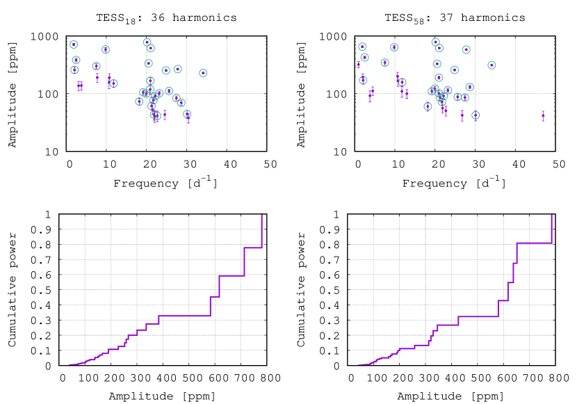
Figure 3: All the detected harmonics in the frequency – amplitude plane and their contributions to the total cumulative power.

In Fig. 3, top panels, we plot all the detected harmonics in the frequency – amplitude plane (with uncertainties). Harmonics that were cross-identified by their frequencies are additionally labelled with circles. We can see that in a given TESS sector just a few harmonics miss a counterpart in the another one. Such cases might indicate that the given harmonic is a false positive or vice versa, that the counterpart harmonic failed to overcome the $\rm FAP=5\%$ threshold level.

In the bottom panels of Fig. 3 we plot the cumulative function of the harmonics power $A_{k}^{2}/2$ against the amplitude $A_{k}$. From these graphs we can see that $\sim 70\%$ of the total power (variance) of the compound harmonics signal is contained in just $4$ or $5$ components of largest amplitude ($A_{k}\gtrsim 600$ ppm), while the remaining $\sim 30\%$ of the total power is distributed among the rest ($A_{k}\lesssim 400$ ppm). The total power of the compound signal corresponds to $\sim 1200$ ppm for TESS₁₈ and TESS₅₈ both.

Table 2: Estimated noise parameters.

Parameter		TESS18	TESS58
$\sigma_{0}$	[ppm]	$260.4(5.3)$	$544.6(4.9)$
$\sigma_{1}$	[ppm]	$525(47)$	$294(23)$
$\tau_{1}$	[d]	$0.52(13)$	$0.230(98)$
$P^{\prime}_{1}$	[d]	$1.65(23)$	$\infty(\gtrsim 1.7)$
$\sigma_{2}$	[ppm]	$426(23)$	$470(22)$
$\tau_{2}$	[d]	$0.182(26)$	$0.182(21)$
$P^{\prime}_{2}$	[d]	$0.1085(15)$	$0.1084(13)$

Table 2 contains the best fitting NWN parameters of the model (2). The total noise variance corresponds to $\sim 700$ ppm and appears nearly the same for TESS₁₈ and TESS₅₈. Within it, the second NWN term appears nearly the same, although the first one reveals a significant change between the sectors, as well as the WN term does. But because of the stable total variance, this difference looks like a power exchange between the WN and the first NWN term over time. The total model variance becomes therefore $\sim 1400$ ppm for the both TESS sectors, and the variance of these data themselves matches this level closely, confirming that our models are consistent and close to being statistically exhaustive.

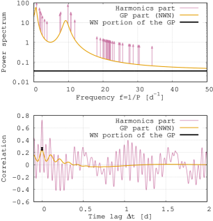
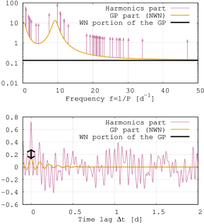
Figure 4: Power spectrum and correlation function of the compound model “harmonics+NWN”.

Finally, in Fig. 4 we show the power spectrum of the compound model “harmonics + NWN”, as well as its correlation function. The power spectrum is normalized so that it can be directly compared with the periodograms in Fig. 2. The NWN has a continuous power spectrum, but harmonics are expressed by delta functions there, so we plot them as vertical arrows starting from the NWN graph. In the correlation function plots we show separate graphs for the WN and NWN portions, and for the harmonics. Notice that correlation function of a single sinusoid in (1) is $\frac{A_{k}^{2}}{2}\cos 2\pi f_{k}\Delta t$.

4 Improving transit timing accuracy

Now let us consider how our out-of-transit photometric model of WASP-33 can be used to detrend the transit lightcurves. The most direct and robust way to achieve this is to fit the entire TESS dataset (OTD and ITD) with this model, augmented by the models of all the transits. However, this way it would require too slow nonlinear fits, and besides we have a goal in mind to employ our model with any other transit observations, so it is necessary to develop an approach that avoids using full TESS data directly.

Our model contains two components: the deterministic one $\mu(t)$ (harmonics) and the GP part (NWN) expressed by the correlation function $k(\Delta t)$. Regarding the deterministic part, its uncertainty can be computed based on the covariance matrix of fitted parameters. This uncertainty remains in the range $100$ ppm to $250$ ppm (for TESS₁₈ and TESS₅₈, resp.) Relatively to the average TESS-reported uncertainty for these data, $\sim 30000$ ppm, this appears below $1\%$. Therefore, possible uncertainty in $\mu(t)$ is surely negligible in comparison with the best expected photometric accuracy. So we can simply subtract our best fitting $\mu(t)$ from the ITD, as if it was a predefined function. We will refer this part of the ITD processing as detrending for shortness.

Regarding the NWN part of the model, its smallest $\tau_{k}$ from Table 2 are about $3$-$4$ h, which is similar to the exoplanet transit duration. This makes it tentative to construct some kind of a GP prediction model (based on the OTD subset) and then to subtract it from the ITD, just like $\mu(t)$. We undertook an attempt to compute an OTD-conditioned GP predictive model with parameters taken from Table 2. However, the practical predictability timescale appeared significantly smaller than $\tau_{k}$, namely below $1$ h. Along the transit duration the variance of this prediction remained mostly close to the total variance of the NWN (i.e. to the unconditional variance, as if OTD were not used). Therefore, such a predictive model would not be very helpful, but simultaneously this means that we would not loose significant information if we do not use the OTD directly when processing the ITD. This enabled us to apply a simplified approach with maximum-likelihood fitting of the ITD adopting a fixed covariance matrix (which is defined by the NWN parameters from Table 2).

Importantly, this approach is equivalent to the whitening in which the data are passed through a linear transform that renders them white. With our GP-fitting algorithm it is unnecessary to apply whitening transform explicitly, but nonetheless we will refer this part of ITD processing as whitening.

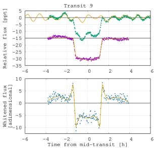
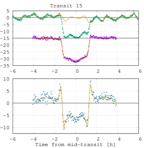
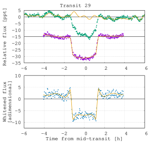
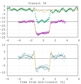
Figure 5: Detrending and whitening for a few WASP-33 b transits. Notice that whitening normalizes the data to unit variance, therefore changing their scale.

Summarising, our ITD processing consists of two cleaning steps, detrending and whitening. In Fig. 5 we show how they work for a few sample transits. In these graphs we plot the TESS data before processing (green points), the sum-of-harmonics $\mu$ (orange curve), the detrended ITD (black points, shifted down) together with transit model (orange curve), and detrended and whitened ITD, also together with their model (which is also whitened). One can see that detrending can remove a large portion of the host star variability, however some residual nuisance variation still remains and should be removed by whitening.

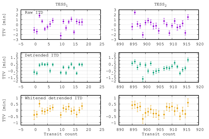
Figure 6: WASP-33 transit timing residuals before and after ITD cleaning. Notice the different ordinate range in the plots.

The effect of this cleaning on transit timings is demonstrated in Fig. 6, where we plot the TTV residuals derived from the initial (raw) ITD, detrended ITD and detrended and whitened ITD. One can see that the TTV scatter is remarkably reduced after each step. The initial TTV residuals r.m.s. was $63$ s. After detrending it became $36$ s, while after the whitening it finally dropped to $18$ s. In total we have a rather dramatic r.m.s. improvement by a factor of $3.5$. The last best-accuracy set of transit timings is given in Table 3.

Table 3: WASP-33 b transit timings derived from the TESS ITD.

Count	Transit midtime	Uncertainty		Count	Transit midtime	Uncertainty
	${\rm BJD}_{\rm TDB}-2450000$	[$\mu$d]			${\rm BJD}_{\rm TDB}-2450000$	[$\mu$d]
$0$	$8791.414033$	$258$		$895$	$9883.198702$	$201$
$1$	$8792.633937$	$159$		$896$	$9884.418601$	$205$
$2$	$8793.854400$	$174$		$897$	$9885.638313$	$241$
$3$	$8795.073868$	$164$		$898$	$9886.858240$	$231$
$4$	$8796.293701$	$147$		$899$	$9888.077415$	$253$
$5$	$8797.513646$	$157$		$900$	$9889.297622$	$231$
$6$	$8798.733608$	$167$		$901$	$9890.517557$	$206$
$7$	$8799.953546$	$148$		$902$	$9891.737565$	$218$
$10$	$8803.612735$	$147$		$903$	$9892.957195$	$218$
$11$	$8804.832992$	$168$		$904$	$9894.177067$	$218$
$12$	$8806.052801$	$157$		$905$	$9895.396842$	$239$
$13$	$8807.272817$	$170$		$907$	$9897.836623$	$208$
$14$	$8808.492430$	$172$		$908$	$9899.056929$	$208$
$15$	$8809.712358$	$180$		$909$	$9900.276759$	$216$
$16$	$8810.931984$	$149$		$910$	$9901.496689$	$210$
$17$	$8812.152104$	$156$		$911$	$9902.716297$	$222$
$18$	$8813.372200$	$167$		$912$	$9903.936334$	$180$
				$913$	$9905.155748$	$191$
				$914$	$9906.375930$	$204$
				$915$	$9907.595621$	$220$
				$916$	$9908.816126$	$217$

After that we investigated our improved timing data for possible variations, but with a null result: we did not find any significant quadratic term in the TTV trend and we did not find any significant periodic TTV.

Table 4: Best fitting WASP-33 system parameters.

Planet				Star				Limb darkening
$P$	[d]	$1.219870529(69)$		$M_{\star}$	[$M_{\odot}$]	$1.495(31)$	∗∗	$A$	$0.215(32)$
$l$	[∘]	$86.4122(99)$	∗	$R_{\star}$	[$R_{\odot}$]	$1.510(12)$		$B$	$0.092(51)$
$i$	[∘]	$87.19(47)$		$\rho_{\star}$	[$\rho_{\odot}$]	$0.4340(59)$		$A_{\rm I}$	$0.1883$
$r/R_{\star}$		$0.11078(23)$						$B_{\rm I}$	$0.2873$
$r$	[$R_{\rm Jup}$]	$1.665(15)$						$A_{\rm II}$	$0.246(6)$
$a$	[AU]	$0.02555(35)$						$B_{\rm II}$	$0.252(6)$

${}^{*\phantom{*}}$ Epoch $\rm BJD_{TDB}=2459000$.

^∗∗ Taken from (Collier Cameron et al., 2010).

Finally, fitting the detrended and whitened ITD allowed us to obtain an improved set of WASP-33 system parameters. They are given in Table 4. This fit used the stellar mass estimate by Collier Cameron et al. (2010), but ignored their stellar radius since we need to know the correlation between $M_{\star}$ and $R_{\star}$ to correctly include them both. Our estimate for the stellar density appeared somewhat smaller though (by $\sim 2.5\sigma$).

We treated the limb darkening coefficients as fittable parameters, but for a comparison in Table 4 we also give their reference values (i) computed from the tables by Claret (2017) using $T_{\rm eff}$, $\log g$, and $[Fe/H]$ by Collier Cameron et al. (2010) and (ii) computed by von Essen et al. (2020). These reference sets both differ from the fitted one, as well as from each other. This may indicate some issues regarding their reliability for not yet clear reasons.

5 Discussion

The approach based on the explicit modelling of WASP-33 variability appears extremely successful in improving its exoplanet transit timings accuracy. In total, we obtained a dramatic TTV r.m.s. improvement by a factor of $3.5$. However, it is important that we must take into account the deterministic as well as non-deterministic (NWN) parts of this variability. Both of them incorporate a similar amount in the total TTV error budget.

Our results still cannot be directly applied to observations from other sites than TESS, because the model parameters somewhat change on the timescale of a few years. Because of that we cannot use TESS-derived model with data obtained e.g. years prior to TESS. However, the frequencies of the harmonics and of the QP part of the NWN look stable, so it may be possible to apply our model to ground-based WASP-33 photometry assuming that only these frequencies are fixed and to refit harmonics amplitudes and phases, as well as NWN variances. But possible ways to reprocess old data using TESS-based models need more investigation.

Our results regarding the set of frequencies in the deterministic part of the WASP-33 variability are generally similar to von Essen et al. (2020). We found $43$ harmonics in total, although only $30$ of them are surely reliable because they were revealed in the both datasets, TESS₁₈ and TESS₅₈. von Essen et al. (2020) detected $29$ harmonics in TESS₁₈, which is nearly the same number. However, there are a few individual differences. Based on our analysis we cannot confirm that their harmonics F21, F25, and F29 are statistically significant, even in a single TESS sector. On contrary, our harmonics H22, H32, H37, and H40 were revealed both in TESS₁₈ and TESS₅₈, but left undetected by von Essen et al. (2020). Among our harmonics that were revealed in TESS₁₈, but not in TESS₅₈, only one (H3 = F28) appeared in von Essen et al. (2020). Among harmonics that were detected in TESS₅₈, but not in TESS₁₈, none appeared in von Essen et al. (2020). This may render our $13$ “single-sector” harmonics less reliable, although this does not necessarily mean that all of them, or their majority, are false positives. Based on our FAP threshold of $5\%$, the expected number of false positives after $36$ or $37$ applications of the significance test should be just one or two (for each TESS sector). And these false positives are, most probably, among the “single-sector” harmonics.

Regarding the secondary eclipses of WASP-33 b, detected by von Essen et al. (2020), we cut them away from our OTD, so they did not affect our analysis and we did not consider them here. But two other planet-related effects reported by (von Essen et al., 2020), namely the orbital phase variation and the ellipsoidal variation, could affect our results, so we included them in the model $\mu$ from the beginning of our analysis. For the orbital phase variation our final amplitude estimate was $(110\pm 100)$ ppm and $(32\pm 44)$ ppm (resp. in TESS₁₈ and TESS₅₈), while von Essen et al. (2020) gave $(100.4\pm 13.1)$ ppm. We can see a large disagreement in the uncertainty, most probably related to the different NWN treatment by von Essen et al. (2020) which we believe was oversimplified. Based on our analysis we cannot confirm that there is a statistically significant evidence in favour of the orbital phase variation in TESS observations. For the ellipsoidal variation we obtained amplitude estimations of $(65\pm 41)$ ppm and $(97\pm 31)$ ppm, for the two TESS sectors. von Essen et al. (2020) gave $27.4$ ppm in the text, although we think this could be a typo, because from their Fig. 9 this amplitude follows to be $\sim 40$ ppm. In any case, their value was theoretically predicted rather than estimated from the data directly. The value of $\sim 40$ ppm is within at most two-sigma from our estimations. As we can see, in our analysis this effect comparable to the uncertainty and cannot be reliably confirmed observationally.

Data availability

The data underlying this article are available in the MAST (Mikulski Archive for Space Telescopes), at https://archive.stsci.edu/, in the article and in its online supplementary material.

References

- Antoci et al. (2019) Antoci V., et al., 2019, MNRAS, 490, 4040
- Baglin et al. (1973) Baglin A., Breger M., Chevalier C., Hauck B., Le Contel J. M., Sareyan J. P., Valtier J. C., 1973, A&A, 23, 221
- Baluev (2008) Baluev R. V., 2008, MNRAS, 385, 1279
- Baluev (2009) Baluev R. V., 2009, MNRAS, 393, 969
- Baluev (2011) Baluev R. V., 2011, Celest. Mech. Dyn. Astron., 111, 235
- Baluev (2013a) Baluev R. V., 2013a, Astron. & Comput., 2, 18
- Baluev (2013b) Baluev R. V., 2013b, MNRAS, 429, 2052
- Baluev (2015) Baluev R. V., 2015, MNRAS, 446, 1493
- Baluev (2018) Baluev R. V., 2018, Astron. & Comput., 25, 221
- Borucki et al. (2010) Borucki W. J., et al., 2010, Science, 327, 977
- Breger (1979) Breger M., 1979, PASP, 91, 5
- Breger & Stockenhuber (1983) Breger M., Stockenhuber H., 1983, Hvar Observ. Bull., 7, 283
- Breger et al. (1999) Breger M., et al., 1999, A&A, 349, 225
- Campbell & Wright (1900) Campbell W. W., Wright W. H., 1900, ApJ, 12, 254
- Chakrabarty & Sengupta (2019) Chakrabarty A., Sengupta S., 2019, AJ, 158, 39
- Claret (2017) Claret A., 2017, A&A, 600, A30
- Colacevich (1935) Colacevich A., 1935, PASP, 47, 231
- Collier Cameron et al. (2010) Collier Cameron A., et al., 2010, MNRAS, 407, 507
- Cox (1963) Cox J. P., 1963, ApJ, 138, 487
- Csizmadia et al. (2023) Csizmadia S., Smith A. M. S., Kálmán S., Cabrera J., Klagyivik P., Chaushev A., Lam K. W. F., 2023, A&A, 675, A106
- Delisle et al. (2020) Delisle J. B., Hara N., Ségransan D., 2020, A&A, 635, A83
- Eggen (1956) Eggen O. J., 1956, PASP, 68, 238
- Fath (1935) Fath E., 1935, PASP, 47, 232
- Foster (1995) Foster G., 1995, AJ, 109, 1889
- Garg et al. (2010) Garg A., et al., 2010, AJ, 140, 328
- Herrero et al. (2011) Herrero E., Morales J. C., Ribas I., Naves R., 2011, A&A, 526, L10
- Kálmán et al. (2022) Kálmán S., Bókon A., Derekas A., Szabó G. M., Hegedűs V., Nagy K., 2022, A&A, 660, L2
- Lomb (1976) Lomb N. R., 1976, Ap&SS, 39, 447
- Milligan & Carson (1992) Milligan H., Carson T. R., 1992, Ap&SS, 189, 181
- Poleski et al. (2010) Poleski R., et al., 2010, Acta Astronomica, 60, 1
- Scargle (1982) Scargle J. D., 1982, ApJ, 263, 835
- von Essen et al. (2014) von Essen C., et al., 2014, A&A, 561, A48
- von Essen et al. (2020) von Essen C., Mallonn M., Borre C. C., Antoci V., Stassun K. G., Khalafinejad S., Tautvaišienė G., 2020, A&A, 639, A34