An Adaptive Space-Time Method for Nonlinear Poroviscoelastic Flows with Discontinuous Porosities

Abstract.

This paper is concerned with a space-time adaptive numerical method for instationary porous media flows with nonlinear interaction between porosity and pressure, with focus on problems with discontinuous initial porosities. A convergent method that yields computable error bounds is constructed by a combination of Picard iteration and a least-squares formulation. The adaptive scheme permits spatially variable time steps, which in numerical tests are shown to lead to efficient approximations of solutions with localized porosity waves. The method is also observed to exhibit optimal convergence with respect to the total number of spatio-temporal degrees of freedom.

1. Introduction

In porous media flows, important transient effects can arise from nonlinear interactions of porosity and pressure, which in certain cases can lead to the formation of porosity waves. These can take the form of solitary waves formed by travelling higher-porosity regions [21] or of chimney-like channels [15]. Such effects are important, for instance, in the modelling of rising magma [12, 2], where porosity waves arise due to high temperatures. Such waves or channels can also form in soft sedimentary rocks, in salt formations or under the influence of chemical reactions; see for example [20, 16, 15]. Quantifying uncertainties caused by the formation of preferential flow pathways can thus be important for safety analyses in geoengineering applications [23].

1.1. Poroviscoelastic model

We consider the instationary poroviscoelastic model analyzed in [1] that can be regarded as a generalization of the models introduced in [4, 19] for the interaction of porosity $\phi$ and effective pressure $u$. Throughout, we assume a spatial domain $\Omega\subseteq\mathbb{R}^{d}$ with $d\in\mathbb{N}$ to be given. For $T>0$, we write $\Omega_{T}=(0,T)\times\Omega$. The model for a poroviscoelastic flow on which we focus in this work reads

$$\partial_{t}\phi =-(1-\phi)\left(\frac{b(\phi)}{\sigma(u)}u+Q\partial_{t}u\right),$$ (1.1a)

$$\partial_{t}u =\frac{1}{Q}\left(\nabla\cdot a(\phi)(\nabla u+(1-\phi)f)-\frac{b(\phi)}{\sigma(u)}u\right),$$ (1.1b)

with functions $a$, $b$ and $\sigma$ that are to be specified, and where $Q>0$ and $f\in\mathbb{R}^{d}$ are assumed to be given constants. For details on the derivation of (1.1), we refer to [1, Appendix A]. Physically meaningful solutions of this problem need to satisfy $\phi\in(0,1)$ on $\Omega_{T}$. The problem is supplemented with initial data

$$\phi(0,x)=\phi_{0}(x),\quad u(0,x)=u_{0}(x),\quad x\in\Omega,$$ (1.2)

for given functions $\phi_{0}\colon\Omega\to(0,1)$ and $u_{0}\colon\Omega\to\mathbb{R}$, as well as homogeneous Dirichlet boundary conditions for $u$ on $(0,T]\times\partial\Omega$.

The coefficient functions $a$ and $b$ of main interest are of the form

$$a(\phi)=a_{0}\phi^{n},\qquad b(\phi)=b_{0}\phi^{m}$$ (1.3)

with real constants $a_{0},b_{0}>0$ and $n,m\geq 1$. This assumption on $a$ is motivated by the Carman-Kozeny relationship [5] between the porosity $\phi$ and the permeability of the medium. The function $\sigma$ accounts for decompaction weakening [16, 15] and $\sigma/\phi^{m}$ can be regarded as the effective viscosity.

For modelling sharp transitions between materials, it is important to be able to treat porosities with jump discontinuities. These turn out to be determined mainly by the initial datum $\phi_{0}$ for the porosity. As shown in [1], under appropriate conditions on $\phi_{0}$ that permit jump discontinuities, these generally remain present also in the corresponding solution $\phi$, but under the given model cannot change their spatial location.

1.2. Existing numerical methods and novelty

Many different methods have been proposed to solve the above type of problem numerically, for example finite difference schemes with implicit time-stepping in [4] and adaptive wavelets in [19]. In a number of recent works, pseudo-transient schemes based on explicit time stepping in a pseudo-time variable have been investigated. Due to their compact stencils, low communication overhead and simple implementation, such schemes are well suited for parallel computing on GPUs, so that very high grid resolutions can be achieved to compensate the low order of convergence, as shown for example in [17, 16, 15, 14, 22, 18]. Even though all of these schemes are observed to work well for smooth initial porosities $\phi_{0}$, their convergence can be very slow in problems with nonsmooth $\phi_{0}$, in particular in the presence of discontinuities. In such cases, due to the smoothing that is implicit in the finite difference schemes, accurately resolving sharp localized features can require extremely large grids. An example is shown in Figure 1.

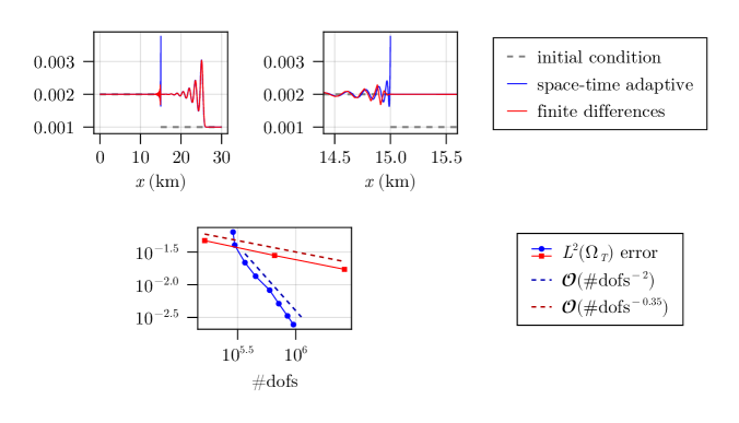
Figure 1. Porosity approximation of space-time adaptive solver with polynomial degree $3$ and finite difference solver (top left) with zoom-in at the discontinuity (top right) and associated convergence rates (bottom; the space-time approximation by the finite difference scheme in the comparison uses a grid with sizes $\Delta t\eqsim\Delta x$, but is computed with smaller intermediate time steps for stability).

We introduce a space-time adaptive method for solving (1.1) based on a combination of Picard iteration for (1.1a) and a particular adaptive least squares discretization of (1.1b). While we focus on this particular model case, the approach can be generalized, for example, to similar problems with full force balance, where (1.1b) is replaced by a time-dependent Stokes problem as in [15].

The adaptive scheme yields efficient approximations of localized features of solutions, in particular in the presence of discontinuities, and can generate space-time grids corresponding to spatially adapted time steps. The method provides a posteriori estimates of the error with respect to the exact solution of the coupled nonlinear system of PDEs. Moreover, we numerically observe optimal convergence rates of the generated discretizations with respect to the total number of degrees of freedom.

1.3. Outline

In Section 2 we describe the basic equations, as well as some possible simplifications and reformulations. We then consider a space-time method for the parabolic equation in Section 3.1 and for the pointwise ODE in Section 3.2, which yields a method for the full coupled problem. The convergence of this method is shown in Section 4, and the resulting adaptively controlled scheme is described in Section 4.5. In Section 5.1 we show numerical results (especially in the case of discontinuities) and in Section 5.2 we numerically investigate the convergence rates of the fully adaptive methods from Section 4.5. At the end we briefly discuss a similar numerical method for the simplified viscous limit model in Section 6.

2. Assumptions and simplified models

In this section we describe the small-porosity approximation as a common simplification and show numerically that it may not be suitable in the case of initial data of low regularity. Based on a transformed version of the general model that facilitates its analysis with non-smooth data, we then state the mild-weak formulation of (1.1) on which our numerical scheme is based.

We start with a crucial assumption on $\sigma$ required for the analysis of (1.1) in [1], which we also rely on in what follows.

Assumptions 1.

We assume that $\sigma\in C^{1}(\mathbb{R})$ satisfies

$$\sup_{v\in\mathbb{R}}\sigma(v)<\infty,\quad\inf_{v\in\mathbb{R}}\sigma(v)>0,\quad\sigma^{\prime}\geq 0\text{ on $\mathbb{R}$},$$

as well as

$$\inf_{v\in\mathbb{R}}\left\{\frac{1}{\sigma(v)}-\frac{v\sigma^{\prime}(v)}{\sigma^{2}(v)}\right\}>0,\quad c_{L}=\sup_{v\in\mathbb{R}}\left\{\frac{1}{\sigma(v)}-\frac{v\sigma^{\prime}(v)}{\sigma^{2}(v)}\right\}<\infty.$$

A trivial example for $\sigma$ fulfilling Assumptions 1 is given by $\sigma(v)=c_{0}$ for all $v\in\mathbb{R}$ with a constant $c_{0}>0$, proposed in [19]. Another example, suggested in [16, 15] and verified to satisfy Assumptions 1 in [1], is

$$\sigma(v)=c_{0}\left(1-c_{1}\left(1+\tanh\left(-\frac{v}{c_{2}}\right)\right)\right),\quad v\in\mathbb{R},$$ (2.1)

which provides a phenomenological model for decompaction weakening. Here $c_{0}>0$ is a positive constant, $c_{1}\in[0,\frac{1}{2})$ and $c_{2}>0$, where $1+\tanh$ can be regarded as a smooth approximation of a step function taking values in the interval $(0,2)$. In most the well-studied case $c_{1}=0$, as considered in [19], one observes the formation of porosity waves, whereas $c_{1}>0$ with appropriate problem parameters and initial conditions can lead to the formation of channels. In what follows, it will be convenient to write

$$\kappa(v)=\frac{v}{\sigma(v)}\,.$$ (2.2)

Note that $\kappa$ is Lipschitz continuous with Lipschitz constant $c_{L}$ by Assumptions 1.

2.1. Small-porosity approximation

For initial data with $\phi_{0}(x)\in(0,1]$ for $x\in\Omega$ and bounded $u$, for a classical solution to (1.1) one has $\phi\leq 1$ due to the presence of the factor $(1-\phi)$ in (1.1a). The small-porosity approximation consists in replacing the factor $(1-\phi)$ in (1.1) by 1, which gives the simplified model

$$\partial_{t}\phi =-\bigl{(}{b(\phi)}{\kappa(u)}+Q\partial_{t}u\bigr{)},$$ (2.3a)

$$\partial_{t}u =\frac{1}{Q}\bigl{(}\nabla\cdot a(\phi)(\nabla u+f)-{b(\phi)}{\kappa(u)}\bigr{)}.$$ (2.3b)

We consider (2.3) subject to the same boundary conditions on $u$ and initial data for $\phi$ and $u$ as for (1.1).

For small $\phi$, it is typically assumed that the qualitative behavior of solutions to (2.3) are similar to the ones of the original model (1.1). However, the small-porosity approximation can lead to unphysical solutions in the case of a discontinuous $\phi_{0}$. This can be seen on the left picture in Figure 2, where starting from typical porosity values of at most $0.2$, the solution develops a peak where $\phi>1$ at the location of the discontinuity. Hence we are interested in keeping the factor $(1-\phi)$ in what follows.

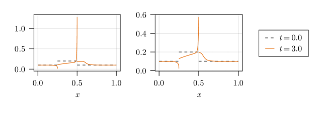
Figure 2. Unphysical solution behavior of the porosity due to the low-porosity approximation (left) and physically correct behavior of the transformed problem (right)

This leads to another difficulty, namely that for the full coupled problem (1.1) with non-smooth initial porosity $\phi_{0}$, the interpretation of the first equation (1.1a) is not obvious, since it contains a term of the form $(1-\phi)\partial_{t}u$. When $\phi$ has jump discontinuities in the spatial variables, $\partial_{t}u$ in general only exists in the distributional sense, that is, as an element of $L_{2}(0,T;H^{-1}(\Omega))$. In this case, the product of the distribution $\partial_{t}u$ and $(1-\phi)$, which is not weakly differentiable, may not be defined. However, the original problem (1.1) including the factor $(1-\phi)$ can be reduced to a similar form as (2.3) by the following observation: (1.1a) can formally be rewritten as

$$\partial_{t}\log(1-\phi)={b(\phi)}{\kappa(u)}+Q\partial_{t}u.$$

Introducing the new variable $\lambda=-\log(1-\phi)$, so that $\phi=1-e^{-\lambda}$, the system (1.1) can be written in the form

$$\partial_{t}\lambda =-\left({b(1-e^{-\lambda})}{\kappa(u)}+Q\partial_{t}u\right),$$ (2.4a)

$$\partial_{t}u =\frac{1}{Q}\left(\nabla\cdot a(1-e^{-\lambda})(\nabla u+e^{-\lambda}f)-{b(1-e^{-\lambda})}{\kappa(u)}\right),$$ (2.4b)

which has the same structure as (2.3). Physically meaningful solutions with $0<\phi<1$ are obtained precisely when $\lambda>0$. As we shall see, the reformulation (2.4) is also advantageous for obtaining a weak formulation, and we will thus consider (1.1) in this form.

Using this transformation, the unphysical behavior shown in Figure 2 can be prevented without changing the general numerical method. The right plot in Figure 2 shows the solution of the transformed problem (2.4) for the same parameters and initial setup, with $\phi<1$ as expected. This shows that it is in general favorable to consider the full model instead of the low-porosity approximation, especially since it does not require more computational effort to solve the transformed problem (2.4).

2.2. Mild and weak formulations

Next we introduce the basic notions of solutions for the different formulations of the problem that we consider in the following sections. The viscoelastic models (2.3) and (2.4) are both of the general form

$$\partial_{t}\varphi =-{\beta(\varphi)}{\kappa(u)}-Q\partial_{t}u,$$ (2.5a)

$$\partial_{t}u =\frac{1}{Q}\left(\nabla\cdot\alpha(\varphi)\bigl{(}\nabla u+\zeta(\varphi)\bigr{)}-{\beta(\varphi)}{\kappa(u)}\right),$$ (2.5b)

where $\alpha,\beta$ and $\zeta$ are given locally Lipschitz continuous functions, with initial conditions $\varphi(0,\cdot)=\varphi_{0}$ and $u(0,\cdot)=u_{0}$ in $\Omega$. Note that since $\varphi$ in (2.5) is in general bounded from above and below, on this range the functions $\alpha,\beta$ and $\zeta$ satisfy a uniform Lipschitz condition.

To give a meaning to these equations for data of low regularity (in particular, when only $\varphi_{0}\in L_{\infty}(\Omega)$ is assumed), we write (2.5a) in integral form and consider (2.5b) in weak formulation. This leads us to the formulation, for a.e. $t\in[0,T]$,

$$\varphi(t,\cdot) =\varphi_{0}+Qu_{0}-Qu(t,\cdot)-\int_{0}^{t}\beta(\varphi\bigl{(}s,\cdot)\bigr{)}\,\kappa\bigl{(}u(s,\cdot)\bigr{)}\,\mathrm{d}s L_{2}(\Omega)$$ in , (2.6a)

$$\partial_{t}u =\frac{1}{Q}\left(\nabla\cdot\alpha(\varphi)\bigl{(}\nabla u+\zeta(\varphi)\bigr{)}-\beta(\varphi)\,\kappa(u)\right) H^{-1}(\Omega)$$ in , (2.6b)

subject to Dirichlet boundary conditions for $u$ and initial data $\varphi(0,\cdot)=\varphi_{0}$, $u(0,\cdot)=u_{0}$ in $\Omega$ for some given $\varphi_{0},u_{0}\in L_{2}(\Omega)$. In addition to Assumptions 1 on $\sigma$ (and hence, in view of (2.2) on $\kappa$), we make the following assumptions on $\alpha$, $\beta$ and $\zeta$ to obtain well-posedness of solutions and convergence of the numerical method.

Assumptions 2.

We assume that $\alpha,\beta,\zeta\in C^{0,1}_{\mathrm{loc}}(\mathbb{R}^{+})$ and that $\alpha$ is strictly positive on $\mathbb{R}^{+}$; in other words, for each $\delta>0$ there exists an $\epsilon>0$ such that for all $x\in[\delta,\infty)$ we have $\alpha(x)\geq\epsilon>0$. Furthermore we assume that $\beta(x)\geq 0$ for each $x\in\mathbb{R}^{+}$.

3. Inexact fixed-point iteration

Similar to the well-posedness results in [1], we perform a Picard iteration for $\varphi$ in order to solve (2.6a). We denote the solution for $u$ given a fixed $\varphi$ by $\mathcal{P}[\varphi]$. The iteration then reads

$$\varphi^{(k+1)}(t,\cdot)=\varphi_{0}-Q(\mathcal{P}[\varphi^{(k)}](t,\cdot)-u_{0})-\int_{0}^{t}\beta(\varphi^{(k)}(s,\cdot))\kappa(\mathcal{P}[\varphi^{(k)}](s,\cdot))\,\mathrm{d}s.$$ (3.1)

One may iterate until reaching a certain tolerance determined, for example, by an a posteriori error estimate based on contractivity. As shown in [1, Sec. 4], the mapping defined by the right-hand side of (3.1) is indeed a contraction for sufficiently small $T$. In the following section, we consider a numerical scheme for (2.6b) for given $\varphi$. We then turn to the discretization of (3.1) in Section 3.2.

3.1. Treatment of the parabolic equation

To solve (2.6b) numerically for a given $\overline{\varphi}$, we linearize it by means of another Picard iteration, which leads to solving

$$\partial_{t}u^{(k)}=\frac{1}{Q}\left(\nabla\cdot\alpha(\overline{\varphi})(\nabla u^{(k)}+\zeta(\overline{\varphi}))-\beta(\overline{\varphi})\,\frac{u^{(k)}}{\sigma(u^{(k-1)})}\right),\quad u^{(k)}(0,\cdot)=u_{0}$$ (3.2)

given the previous iterate $u^{(k-1)}$. We start with an initial iterate $u^{(0)}$ which, unless stated otherwise, will be a constant continuation of $u_{0}$. Following [8, 9], let

$$U:=\left\{(u,\eta)\in L_{2}(0,T;H_{0}^{1}(\Omega))\times L_{2}(\Omega_{T})^{d}\,\colon\,\operatorname{div}(u,\eta)\in L_{2}(\Omega_{T})\right\}$$

with the induced graph norm

$$\|(u,\eta)\|_{U}^{2}=\|(u,\eta)\|_{L_{2}(\Omega_{T},\mathbb{R}^{d+1})}^{2}+\|\nabla_{\!x}u\|_{L_{2}(\Omega_{T},\mathbb{R}^{d})}^{2}+\|\operatorname{div}(u,\eta)\|_{L_{2}(\Omega_{T})}^{2},$$ (3.3)

where $\operatorname{div}(u,\eta):=\partial_{t}u+\operatorname{div}_{x}\eta$ denotes the space-time divergence. Moreover, let

$$V:=L_{2}(\Omega_{T})\times L_{2}(\Omega_{T},\mathbb{R}^{d})\times L_{2}(\Omega),$$

endowed with its canonical norm, and

$$G[\overline{u}](u,\eta):=\begin{pmatrix}\operatorname{div}(u,\eta)+\tilde{\beta}\,\frac{u}{\sigma(\overline{u})}\\ \eta+\tilde{\alpha}\,\nabla_{\!x}u\\ u(0,\cdot)\end{pmatrix},\qquad R:=\begin{pmatrix}0\\ -\tilde{\alpha}\,\zeta\\ u_{0}\end{pmatrix},$$ (3.4)

where we absorbed $\overline{\varphi}$ and $\frac{1}{Q}$ into the coefficients $\tilde{\alpha},\tilde{\beta}\in L_{\infty}$. This allows us to rewrite (3.2) as

$$G\big{[}u^{(k-1)}\big{]}\big{(}u^{(k)},\eta^{(k)}\big{)}=R,$$ (3.5)

similar to [7, 8, 9]. Now [8, Theorem 2.3] yields the following result on the well-posedness of (3.5).

Theorem 3.1.

Let $\overline{u}\in U$ and $\tilde{\alpha},\tilde{\beta}\in L_{\infty}(\Omega_{T})$ with $\tilde{\alpha}$ uniformly positive. Then $G[\overline{u}]:U\to V$ is an isomorphism.

Due to Assumptions 1 and 2, the assumptions of Theorem 3.1 are fulfilled. Furthermore, the norm induced by $G[\overline{u}]$ is equivalent to $\|\cdot\|_{U}$ independently of $\overline{u}$ due to the uniform boundedness of $\sigma$ from above and below.

Similar to [9], we discretize $U$ by partitioning $\Omega$ and $(0\,,T)$ separately, which leads to a partition $\mathcal{T}$ of prisms. In this work we focus on the case of cubic elements to discretize $\Omega$, which leads to the definition of ($d+1$)-dimensional cubes $\textbf{I}:=I_{1}\times\ldots\times I_{d+1}\in\mathcal{T}$ where $I_{d+1}$ denotes the temporal direction. Hence we write $\textbf{I}_{x}:=I_{1}\times\ldots\times I_{d}$ and define local shape functions

$$\mathcal{S}_{\ell,k}(\textbf{I}):=\big{(}\mathbb{Q}_{k}(\textbf{I}_{x})\otimes\mathbb{P}_{\ell+1}(I_{d+1})\big{)}\times\big{(}\mathrm{RT}_{k}(\textbf{I}_{x})\otimes\mathbb{P}_{\ell}(I_{d+1})\big{)}$$

on $\textbf{I}\in\mathcal{T}$ as in [9, Sec. 2] where $\mathbb{P}_{k}(I)$, $I\subseteq\mathbb{R}$ denotes polynomials of degree $k$ and

$$\begin{split}\mathbb{Q}_{k_{1},\ldots,k_{d}}(\textbf{I}_{x})&:=\mathbb{P}_{k_{1}}(I_{1})\otimes\ldots\otimes\mathbb{P}_{k_{d}}(I_{d}),\\ \mathbb{Q}_{k}&:=\mathbb{Q}_{k,\ldots,k}(\textbf{I}_{x}),\\ \mathrm{RT}_{k}(\textbf{I}_{x})&:=\mathbb{Q}_{k+1,k,\ldots,k}(\textbf{I}_{x})\times\ldots\times\mathbb{Q}_{k,\ldots,k,k+1}(\textbf{I}_{x}).\end{split}$$ (3.6)

Then we consider the conforming subspace

$$U_{\delta}(\mathcal{T}):=\big{\{}(u_{\delta},\eta_{\delta})\in H^{1}(0,T;H^{1}_{0}(\Omega))\times L_{2}(0,T;H_{\operatorname{div}_{x}}(\Omega))\,\colon\\ (u_{\delta},\eta_{\delta})|_{\textbf{I}}\in\mathcal{S}_{\ell,k}(\textbf{I}),\textbf{I}\in\mathcal{T}\big{\}}.$$

In the case of axis-parallel cubes with trivial normal vectors, the conformity corresponds to $u_{\delta}$ being continuous and $(\eta_{\delta})_{i}$ being continuous in the $i$-th spatial direction. As proposed in [9, Sec. 2], we will restrict ourselves to the optimal polynomial degrees $\ell+1=k$ in order to achieve better convergence rates.

We solve (3.5) numerically for fixed $\overline{u}$ in the least-squares formulation of [7, 8, 9], which adapted to the present case, in terms of the definitions in (3.4), reads

$$(u_{\delta},\eta_{\delta})=\operatorname*{arg\,min}_{(v_{\delta},\mu_{\delta})\in U_{\delta}}\|G[\overline{u}](v_{\delta},\mu_{\delta})-R\|_{V}\,.$$ (3.7)

With the associated bilinear form $\Lambda$ and right-hand side $l$ given by

$$\Lambda((u_{\delta},\eta_{\delta}),(v_{\delta},\mu_{\delta}))=\langle G[\overline{u}](u_{\delta},\eta_{\delta})\,,G[\overline{u}](v_{\delta},\mu_{\delta})\rangle_{V},\quad l(v_{\delta},\mu_{\delta})=\langle R\,,G[\overline{u}](v_{\delta},\mu_{\delta})\rangle_{V}\,,$$

the solution $(u_{\delta},\eta_{\delta})\in U_{\delta}$ of (3.7) is characterized by

$$\Lambda((u_{\delta},\eta_{\delta}),(v_{\delta},\mu_{\delta}))=l(v_{\delta},\mu_{\delta})\quad\text{for all $(v_{\delta},\mu_{\delta})\in U_{\delta}$.}$$

Since the residual is evaluated in the $L_{2}$-space $V$, its $L_{2}$-norms on elements of $\mathcal{T}$ yield reliable and computable local error estimators that can be used to drive an adaptive refinement routine. By Theorem 3.1, we furthermore have an equivalence between error and residual,

$$\|(u,\eta)-(u_{\delta},\eta_{\delta})\|_{U}\eqsim\|G[\overline{u}](u_{\delta},\eta_{\delta})-R\|_{V}\,,$$ (3.8)

for $\|\cdot\|_{U}$ defined in (3.3).

Remark 3.2.

It is possible to linearize (2.6b) differently by performing a linearization of the term $\frac{u}{\sigma(u)}$ in $\overline{u}$, which yields

$$\partial_{t}u=\nabla\cdot\tilde{\alpha}(\overline{\varphi})(\nabla u+\zeta(\overline{\varphi}))-\tilde{\beta}(\overline{\varphi})\left(\frac{u}{\sigma(\overline{u})}-\frac{\overline{u}\,\sigma^{\prime}(\overline{u})}{\sigma(\overline{u})^{2}}(u-\overline{u})\right),\quad u(0,\cdot)=u_{0}.$$ (3.9)

The resulting Gauß-Newton-type iteration generally converges faster in general than the simpler quasilinear iteration in (3.2).

To this end we introduce the discrete parabolic solution operator $\mathcal{P}_{\delta}$ which is used in the subsequent sections.

Definition 3.3.

We define $\mathcal{P}_{\delta}[\overline{\varphi},\overline{u}]:=(u_{\delta},\eta_{\delta})$ to be the solution of (3.7) up to a tolerance $\mathrm{tol}_{\mathrm{lsq}}>0$ and set

$$\mathcal{P}_{\delta}[\overline{\varphi}]:=(u_{\delta}^{(\ell)},\eta_{\delta}^{(\ell)})=\mathcal{P}_{\delta}[\overline{\varphi},u_{\delta}^{(\ell-1)}]$$ (3.10)

such that $\big{\|}G[u_{\delta}^{(\ell)}](u_{\delta}^{(\ell)},\eta_{\delta}^{(\ell)})-R\big{\|}_{V}\leq\mathrm{tol}_{u}$ holds for some given tolerance $\mathrm{tol}_{u}\geq\mathrm{tol}_{\mathrm{lsq}}>0$.

3.2. A space-time adaptive fixed-point method

To approximate $\varphi$, we aim to discretize (3.1) while maintaining convergence of the fixed-point iteration. This can be done using (3.11), where we consider a given approximation $\mathcal{P}_{\delta}[\varphi_{\delta}^{(k)}]$ of $\mathcal{P}[\varphi_{\delta}^{(k)}]$ from Definition 3.3 on some adaptively refined space-time grid. Then we compute

$$\begin{split}\varphi_{\delta}^{(k+1)}=&\,\Pi\bigg{(}\varphi_{0}-Q\Big{(}\mathcal{P}_{\delta}[\varphi_{\delta}^{(k)}](t,\cdot)-u_{0}\Big{)}\\ &\phantom{\,\Pi\bigg{(}}-\int_{0}^{t}\mathcal{I}\Big{(}\beta(\varphi_{\delta}^{(k)}(s,\cdot))\,\kappa(\mathcal{P}_{\delta}[\varphi_{\delta}^{(k)}](s,\cdot))\Big{)}\,\mathrm{d}s\bigg{)},\end{split}$$ (3.11)

where $\mathcal{I}$ denotes interpolation with high-order polynomials (using Chebyshev nodes) such that the resulting error is bounded by a given tolerance $\mathrm{tol}_{\mathrm{int}}>0$. Then we perform exact integration of the polynomial approximations. Note that it is important for this step to merge the grids for $u_{\delta}$ and $\varphi_{\delta}^{(k)}$ first and make them uniform in time (that means without hanging nodes on time-facets) such that we can calculate the integral without running into problems with possible discontinuities in space.

The resulting high-order polynomial on a time-uniform grid is projected to a lower-order polynomial on an adaptive grid by a projection $\Pi$ such that the error is bounded by $\mathrm{tol}_{\mathrm{proj}}>0$. For this step we use an adaptive $L_{2}$-projection based on the $h$-adaptive approximation method derived in [3, Sec. 2], which aligns with the theory developed in Section 4.2. This projection is chosen in a specific way to allow for a temporal decomposition of $\Omega_{T}$ discussed in Sections 3.3 and 4.4.

Next we combine the above steps in an adaptive scheme for the full nonlinear problem (2.6).

Algorithm 1 Full Method to solve (2.5)

0:  $\mathrm{tol}_{\varphi}$, $\mathrm{tol}_{\mathrm{proj}}$, $\mathrm{tol}_{\mathrm{int}}$, $\mathrm{tol}_{u}$, $\mathrm{tol}_{\mathrm{lsq}}$, $u_{0}$, $\varphi_{0}$

0:  $\varphi_{\delta}$, $u_{\delta}$

  initialize $\varphi_{\delta}^{(0)}$

  while $\mathrm{res}_{\varphi}>\mathrm{tol}_{\varphi}$ do

     initialize $u_{\delta}^{(0)}$

     while $\mathrm{res}_{u}>\mathrm{tol}_{u}$ do

        solve $u_{\delta}^{(\ell+1)}=\mathcal{P}_{\delta}[\varphi_{\delta}^{(k)},u_{\delta}^{(\ell)}]$ up to $\mathrm{tol}_{\mathrm{lsq}}$

        compute $\mathrm{res}_{u}=\big{\|}G[u_{\delta}^{(\ell+1)}](u_{\delta}^{(\ell+1)},\eta_{\delta}^{(\ell+1)})-R\big{\|}_{V}$

     end while

     calculate $\varphi_{\delta}^{(k+1)}$ by (3.11) up to $\mathrm{tol}_{\mathrm{proj}}$, $\mathrm{tol}_{\mathrm{int}}$

     estimate $\mathrm{res}_{\varphi}\lesssim\big{\|}\varphi_{\delta}^{(k+1)}-\varphi_{\delta}^{(k)}\big{\|}_{T}$

  end while

There are different ways of combining the methods from Sections 3.1 and 3.2, but the most reliable one coincides with the theoretical ideas from [1] and is summarized in Algorithm 1. There we solve for $\mathcal{P}_{\delta}[\varphi_{\delta}]$ and then update $\varphi_{\delta}$ until the respective error tolerances are fulfilled where the norm $\|\cdot\|_{T}$ is going to be specified in Section 3.3. A more involved scheme for controlling these tolerances themselves adaptively is presented in Section 4.5.

3.3. Temporal subdivision

To ensure convergence of the nonlinear iterations (3.1) and (3.2), in general we need to split the space-time cylinder $\Omega_{T}$ into time slices that can be chosen as large as the Lipschitz constants of both iterations allow. Hence their size only depends on the continuous problem, but is independent of the discretization. However, to maintain control of overall errors, controlling the trace errors at time slice boundaries is crucial.

Hence doing this re-approximation simply in the norm of $L_{2}(\Omega_{T})$ is not sufficient for controlling the resulting errors of $\gamma_{T}\varphi_{\delta}$ in $L_{2}(\Omega)$-norm, where $\gamma_{t}:f\mapsto f(t,\cdot)$ is the associated trace operator for each time $t\in[0,T]$. It clearly is bounded as a mapping from $C([0,T];L_{2}(\Omega))$ to $L_{2}(\Omega)$ and as a mapping from $U$ to $L_{2}(\Omega)$, since for the scalar components of elements of $U$ we can apply [8, Proposition 2.1] and the imbedding

$$L_{2}(0,T;H^{1}_{0}(\Omega))\cap H^{1}(0,T;H^{-1}(\Omega))\hookrightarrow C([0,T];L_{2}(\Omega)).$$ (3.12)

We thus modify the re-approximation to explicitly account for errors in the trace at $T$ as follows. Given a partition of $\mathcal{T}$ of $\Omega_{T}$ into prisms, where $\mathbb{Q}_{k_{1},\ldots,k_{d+1}}$ denotes the space-time tensor polynomial space defined in (3.6), we define $X_{\delta}(\mathcal{T})=\{f\in L_{2}(\Omega_{T})\,\colon f|_{e}\in\mathbb{Q}_{k_{1},\ldots,k_{d+1}}(e)\text{ for all }e\in\mathcal{T}\}$. Then the projection $\Pi$ is defined as

$$\Pi f:=\operatorname*{arg\,min}_{f_{\delta}\in X_{\delta}(\mathcal{T})}\|f-f_{\delta}\|_{T},$$

where

$$\|f\|_{T}^{2}:=\|f\|_{L_{2}(\Omega_{T})}^{2}+\|\gamma_{T}f\|_{L_{2}(\Omega)}^{2}$$ (3.13)

defines a norm on $C([0,T];L_{2}(\Omega))$. Note that $\|\cdot\|_{T}$ is induced by an $L_{2}$-inner product and hence it is easy to compute the minimizer in the definition of $\Pi$. Combining this with the adaptive tree refinement of [3, Sec. 2], we obtain a near-best approximation tree. Together with the estimates derived in Sections 4.1 and 4.2 we can control the terminal nonlinear errors of $\varphi$ and $u$.

Rather than splitting the domain into time slices, one could also consider a globally coupled approach by solving for subsets of unknowns while freezing the remaining ones. However, due to the global coupling in time in the discretization of the (generally nonlinear) parabolic problem for $u$, convergence of iterations constructed in this manner is a delicate question. It becomes easier in cases where the parabolic problem is linear, for example when $\sigma$ is constant, but since this is a strong restriction excluding problems with decompaction weakening that are of main interest to us, we do not pursue this direction further.

4. Convergence

In order to prove the convergence of Algorithm 1, we start by considering a convergence result for an abstract perturbed fixed-point iteration that we subsequently apply to our method. We assume that $\Xi$ is a Lipschitz continuous mapping with Lipschitz constant $L_{\psi}<1$ with respect to a suitable norm on a suitably chosen closed set, which implies that Banach’s fixed point theorem yields a unique fixed point $\psi$ as well as convergence of the fixed point iteration. Then we can write a discretized iteration in the form

$$\psi_{\delta}^{(k+1)}=\Xi(\psi_{\delta}^{(k)})+\varepsilon_{\delta}^{(k)}\,,$$ (4.1)

where $\varepsilon_{\delta}^{(k)}$ denotes the discretization error. For the resulting error, we then have $\big{\|}\psi-\psi_{\delta}^{(k+1)}\big{\|}\leq L_{\psi}\big{\|}\psi-\psi_{\delta}^{(k)}\big{\|}+\big{\|}\varepsilon_{\delta}^{(k)}\big{\|}\,,$ and thus by induction

$$\big{\|}\psi-\psi_{\delta}^{(k+1)}\big{\|}\leq(L_{\psi})^{k+1}\big{\|}\psi-\psi_{\delta}^{(0)}\big{\|}+\sum_{i=0}^{k}(L_{\psi})^{k-i}\big{\|}\varepsilon_{\delta}^{(i)}\big{\|}\,.$$ (4.2)

Furthermore, it is clear that the perturbed fixed point iteration converges if $\big{\|}\varepsilon_{\delta}^{(i)}\big{\|}\rightarrow 0$ for $i\to\infty$. Concerning the speed of convergence, we have the following estimate.

Lemma 4.1.

If for some $\xi<1-L_{\psi}$ and all $k\leq N$,

$$\big{\|}\varepsilon_{\delta}^{(k)}\big{\|}\leq\xi\,(L_{\psi}+\xi)^{k}\,\big{\|}\psi-\psi_{\delta}^{(0)}\big{\|},$$ (4.3)

then $\big{\|}\psi-\psi_{\delta}^{(k)}\big{\|}\leq(L_{\psi}+\xi)^{k}\big{\|}\psi-\psi_{\delta}^{(0)}\big{\|}$ for $k\leq N+1$.

Proof.

With (4.2) we obtain

$$\big{\|}\psi-\psi_{\delta}^{(k+1)}\big{\|} \leq(L_{\psi})^{k+1}\big{\|}\psi-\psi_{\delta}^{(0)}\big{\|}+\sum_{i=0}^{k}(L_{\psi})^{k-i}\big{\|}\varepsilon_{\delta}^{(i)}\big{\|}$$

$$\leq\bigg{(}(L_{\psi})^{k+1}+\xi\sum_{i=0}^{k}(L_{\psi})^{k-i}(L_{\psi}+\xi)^{i}\bigg{)}\big{\|}\psi-\psi_{\delta}^{(0)}\big{\|}$$

$$=(L_{\psi}+\xi)^{k+1}\big{\|}\psi-\psi_{\delta}^{(0)}\big{\|},$$

where in the last step we have used that $(b-a)\sum_{i=0}^{k}a^{k-i}\,b^{i}=b^{k+1}-a^{k+1}$ for $a,b\in\mathbb{R}$ and $k\in\mathbb{N}$. ∎

In what follows, we apply the above to different contractions $\Xi$ with correspondingly different mechanisms for ensuring errors $\big{\|}\varepsilon_{\delta}^{(k)}\big{\|}_{T}$ below the respective thresholds.

4.1. Nonlinear least-squares method

First we want to apply the general results about perturbed fixed-point iterations in order to prove convergence of the nonlinear least-squares method presented in Section 3.1.

We now assume a fixed $\overline{\varphi}$ to be given. Let the operator $\Phi$ be defined, for each given $\overline{u}$, by $\Phi(\overline{u})=u$, where $u$ is the solution of

$$\partial_{t}u=\nabla\cdot\tilde{\alpha}(\overline{\varphi})(\nabla u+\zeta(\overline{\varphi}))-\tilde{\beta}(\overline{\varphi})\,\frac{u}{\sigma(\overline{u})},\quad u(0,\cdot)=u_{0}\,.$$

Lemma 4.2.

For $\Phi$ as defined above, we have

$$\|\Phi(\overline{u}_{2})-\Phi(\overline{u}_{1})\|_{T}\lesssim T^{\frac{1}{2}}\|\overline{u}_{2}-\overline{u}_{1}\|_{L_{2}(\Omega_{T})}\,,$$

which implies that $\Phi$ is a contraction with respect to $\|\cdot\|_{T}$ with Lipschitz constant $L_{u}<1$ if $T$ is sufficiently small.

Proof.

For solutions $u_{1}$ and $u_{2}$ given $\overline{u}_{1}$ and $\overline{u}_{2}$, respectively, we have

$$\partial_{t}(u_{2}-u_{1}) =\nabla\cdot\tilde{\alpha}(\overline{\varphi})\nabla(u_{2}-u_{1})-\tilde{\beta}(\overline{\varphi})\,\left(\frac{u_{2}}{\sigma(\overline{u}_{2})}-\frac{u_{1}}{\sigma(\overline{u}_{1})}\right)$$

$$=\nabla\cdot\tilde{\alpha}(\overline{\varphi})\nabla(u_{2}-u_{1})-\tilde{\beta}(\overline{\varphi})\,\left(\frac{u_{2}-u_{1}}{\sigma(\overline{u}_{2})}+u_{1}\left(\frac{1}{\sigma(\overline{u}_{2})}-\frac{1}{\sigma(\overline{u}_{1})}\right)\right)\,.$$

Using that $\sigma$ is bounded from below and $u_{1}$, $\overline{\varphi}$ uniformly from above, using $\frac{1}{\sigma}\in C^{0,1}(\mathbb{R})$ we obtain the Lipschitz estimate

$$\begin{split}\|u_{2}-u_{1}\|_{L_{2}(\Omega_{T})}&\leq T^{\frac{1}{2}}\|u_{2}-u_{1}\|_{L_{\infty}(0,T;L_{2}(\Omega))}\\ &\lesssim T^{\frac{1}{2}}\Big{\|}\tilde{\beta}(\overline{\varphi})\,u_{1}\left(\tfrac{1}{\sigma(\overline{u}_{2})}-\tfrac{1}{\sigma(\overline{u}_{1})}\right)\Big{\|}_{L_{2}(\Omega_{T})}\\ &\lesssim T^{\frac{1}{2}}\Big{\|}\tfrac{1}{\sigma(\overline{u}_{2})}-\tfrac{1}{\sigma(\overline{u}_{1})}\Big{\|}_{L_{2}(\Omega_{T})}\\ &\lesssim T^{\frac{1}{2}}\|\overline{u}_{2}-\overline{u}_{1}\|_{L_{2}(\Omega_{T})}\,.\end{split}$$ (4.4)

Applying [1, Theorem 4.2] (based on [6]) we immediately get

$$\begin{split}\|u_{2}(T,\cdot)-u_{1}(T,\cdot)\|_{L_{2}(\Omega)}&\leq|\Omega|^{1/2}\|u_{2}(T,\cdot)-u_{1}(T,\cdot)\|_{L_{\infty}(\Omega)}\\ &\lesssim\|u_{2}-u_{1}\|_{L_{2}(\Omega_{T})}\\ &\lesssim T^{\frac{1}{2}}\|\overline{u}_{2}-\overline{u}_{1}\|_{L_{2}(\Omega_{T})}\end{split}$$ (4.5)

with constants independent of $T$. Combining (4.4) and (4.5) yields the desired contraction property. ∎

Noting that the numerical error of our linear least-squares solver can be made arbitrarily small, the numerical method (3.10) converges if $\big{\|}\varepsilon_{\delta}^{(k)}\big{\|}_{T}\leq\mathrm{tol}_{\mathrm{lsq}}^{(k)}\to 0$ for $k\to\infty$. Furthermore, error reduction is obtained by a simpler argument than in Lemma 4.1, ensuring that $\big{\|}\varepsilon_{\delta}^{(k)}\big{\|}_{T}\leq\xi\big{\|}u-u_{\delta}^{(k)}\big{\|}_{T}$ holds for some $\xi<1-L_{u}$. As shown next, this can be guaranteed by considering the nonlinear residual $\|G[u](u,\eta)-G[u_{\delta}](u_{\delta},\eta_{\delta})\|_{V}$, which can be used as an error estimator.

Proposition 4.3.

If $(u_{\delta},\eta_{\delta})$ is a solution of (3.7), then

$$\|(u,\eta)-(u_{\delta},\eta_{\delta})\|_{U}\eqsim\|G[u](u,\eta)-G[u_{\delta}](u_{\delta},\eta_{\delta})\|_{V}.$$ (4.6)

Proof.

We calculate the Fréchet derivative of the nonlinear operator $G[u](u,\eta)$. For $h=(h_{1},h_{2})\in U$ this yields

$$DG[u]h=\begin{pmatrix}\operatorname{div}(h_{1},h_{2})+\tilde{\beta}\frac{\sigma(u)-u\sigma^{\prime}(u)}{\sigma(u)^{2}}h_{1}\\ h_{2}+\tilde{\alpha}\nabla_{\!x}h_{1}\\ h_{1}(0,\cdot)\end{pmatrix}\,,$$

where $\tilde{\beta}\frac{\sigma(u)-u\sigma^{\prime}(u)}{\sigma(u)^{2}}$ is uniformly bounded due to uniform bounds on $\tilde{\beta}$ and Assumptions 1.

By Theorem 3.1, with homogeneous Dirichlet boundary data, $DG[u]:U\to V$ is an isomorphism. Hence we have bounds

$$\|DG[u]\|_{U\to V}\leq C_{1},\quad\|DG[u]^{-1}\|_{V\to U}\leq C_{-1}$$ (4.7)

with $C_{1},C_{-1}>0$ independent of $u$ due to the uniform bounds on $\frac{\sigma(u)-u\sigma^{\prime}(u)}{\sigma(u)^{2}}$. Thus

$$\|G[u](u,\eta)-G[u_{\delta}](u_{\delta},\eta_{\delta})\|_{V}\leq C_{1}\|(u,\eta)-(u_{\delta},\eta_{\delta})\|_{U}\,,$$

which yields one side of the estimate (4.6).

By the bound on $DG^{-1}$ in (4.7), we can apply the inverse function theorem (see, for example, [10, Sec. 9.2]) to conclude that for each $(u,\eta)\in U$ there exists a neighborhood $B$ of $G[u](u,\eta)$ and a unique Fréchet differentiable function $F:B\to U$ such that $G\circ F(x)=x$ and $DF(x)=DG(F(x))^{-1}$ for all $x\in B$. As a consequence of (4.7), we have $\|DF(x)\|_{B\to U}\leq C_{-1}$ for all $x\in B$. Applying the same argument as before to $F$, since $DF(x)^{-1}=DG(F(x))$ is bounded by (4.7), we obtain a unique function $\tilde{G}:\tilde{B}\to B$ such that $F\circ\tilde{G}(u,\eta)=(u,\eta)$ for all $(u,\eta)$ in a neighborhood $\tilde{B}$ of $F(x)$ for $x\in B$. Furthermore, for all $(u,\eta)\in\tilde{B}$,

$$G[u](u,\eta)=G\circ F\circ\tilde{G}(u,\eta)=\tilde{G}(u,\eta)\,.$$

In order to prove the converse estimate in (4.6), we consider the line segment

$$[(u,\eta),(u_{\delta},\eta_{\delta})]:=\left\{\lambda(u,\eta)+(1-\lambda)(u_{\delta},\eta_{\delta})\,\colon\,\lambda\in[0,1]\right\}$$

which is compact in $U$ and hence admits a finite covering of $[(u,\eta),(u_{\delta},\eta_{\delta})]$ by neighborhoods $\tilde{B}$ where $F$ and $\tilde{G}=G$ are defined. We thus obtain a well-defined map $DF$ on the entire line segment, which in addition is uniformly bounded by $C_{-1}$, so that

$$\|(u,\eta)-(u_{\delta},\eta_{\delta})\|_{U} =\|F\circ G[u](u,\eta)-F\circ G[u_{\delta}](u_{\delta},\eta_{\delta})\|_{U}$$

$$\leq C_{-1}\|G[u](u,\eta)-G[u_{\delta}](u_{\delta},\eta_{\delta})\|_{V}\,.$$

∎

Note that due to the imbedding (3.12) this also yields an estimate of $\|u-u_{\delta}^{(\ell)}\|_{T}$.

Theorem 4.4.

Let $\overline{\varphi}$ be fixed, and with $L_{u}$ from Lemma 4.2, let $\xi<1-L_{u}$ and $\mathrm{tol}_{\mathrm{lsq}}$ be chosen such that

$$\big{\|}\varepsilon_{\delta}^{(\ell)}\big{\|}_{T}\leq\xi\,\mathrm{tol}_{\mathrm{lsq}}\lesssim\xi\,\big{\|}G[u_{\delta}^{(\ell)}](u_{\delta}^{(\ell)},\eta_{\delta}^{(\ell)})-R\big{\|}_{V}$$

holds for all $\ell\leq N$, with constant depending on $\|\overline{\varphi}\|_{L_{\infty}(\Omega_{T})}$ and $\|1/\overline{\varphi}\|_{L_{\infty}(\Omega_{T})}$. Then $\big{\|}u-u_{\delta}^{(\ell+1)}\big{\|}_{T}\leq(L_{u}+\xi)\big{\|}u-u_{\delta}^{(\ell)}\big{\|}_{T}$ for $\ell\leq N$, with $u=\mathcal{P}[\overline{\varphi}]$ and $u_{\delta}^{(\ell)}$ as in Definition 3.3.

4.2. Lipschitz estimate

We now show that the operator $\Theta$ defined by

$$\Theta(\varphi)(t,\cdot)=\varphi_{0}-Q\left(\mathcal{P}[\varphi](t,\cdot)-u_{0}\right)-\int_{0}^{t}\beta(\varphi(s,\cdot))\,\kappa(\mathcal{P}[\varphi](s,\cdot))\,\mathrm{d}s,$$

is a contraction with respect to $\|\cdot\|_{T}$ if $T$ is chosen sufficiently small.

In [1, Sec. 4], such a property is established with respect to a piecewise $C^{0,\gamma}_{\textrm{par}}$-norm. With respect to the weaker $T$-norm as used here, contractivity is not known under general assumptions. However, we obtain the desired estimate under the additional assumption that

$$\big{\|}\nabla_{\!x}\mathcal{P}[\varphi_{\delta}^{(k)}]\big{\|}_{L_{\infty}(\Omega_{T})}\leq\overline{C}$$ (4.8)

holds for all $k$. This regularity assumption can be shown, for example, for data with piecewise smooth data, see Remark 4.7; we also observe this to hold in our numerical tests.

Lemma 4.5.

Under the assumption (4.8) it holds that

$$\|\Theta(\varphi_{2})-\Theta(\varphi_{1})\|_{T}\lesssim T^{\frac{1}{2}}\|\varphi_{2}-\varphi_{1}\|_{L_{2}(\Omega_{T})}\,.$$

which implies that $\Theta$ is a contraction with respect to $\|\cdot\|_{T}$ with Lipschitz constant $L_{\varphi}<1$ if $T$ is small enough.

Proof.

Considering a difference equation similar to [1, Sec. 4] we get

$$\partial_{t}(u_{2}-u_{1})-\nabla\cdot(\tilde{\alpha}(\varphi_{1})\nabla(u_{2}-u_{1}))+\tilde{\beta}(\varphi_{1})\Delta_{\kappa,u_{1}}(u_{2})(u_{2}-u_{1})\\ \begin{split}=\;&\nabla\cdot\left((\tilde{\alpha}(\varphi_{2})-\tilde{\alpha}(\varphi_{1}))\nabla u_{2}\right)-\kappa(u_{2})(\tilde{\beta}(\varphi_{2})-\tilde{\beta}(\varphi_{1}))\\ &+\nabla\cdot\left(\tilde{\alpha}(\varphi_{2})\zeta(\varphi_{2})-\tilde{\alpha}(\varphi_{1})\zeta(\varphi_{1})\right)\end{split}$$ (4.9)

where $\Delta_{\kappa,y}$ is defined as

$$\Delta_{\kappa,y}(x):=\begin{cases}\frac{\kappa(x)-\kappa(y)}{x-y}&\text{if }x\neq y,\\ \kappa^{\prime}(y)&\text{else.}\end{cases}$$ (4.10)

By standard regularity theory (see, e.g. [1, Theorem 4.1]), we obtain the estimate

$$\|u_{2}-u_{1}\|_{L_{2}(\Omega_{T})}\\ \begin{split}&\leq T^{1/2}\|u_{2}-u_{1}\|_{L_{\infty}(0,T;L_{2}(\Omega))}\\ &\lesssim T^{1/2}\Big{(}\|(\tilde{\alpha}(\varphi_{2})-\tilde{\alpha}(\varphi_{1}))\,\nabla u_{2}\|_{L_{2}(\Omega_{T})}+\big{\|}\kappa(u_{2})(\tilde{\beta}(\varphi_{2})-\tilde{\beta}(\varphi_{1}))\big{\|}_{L_{2}(\Omega_{T})}\\ &\phantom{\lesssim T^{1/2}\Big{(}}\;+\|\tilde{\alpha}(\varphi_{2})\zeta(\varphi_{2})-\tilde{\alpha}(\varphi_{1})\zeta(\varphi_{1})\|_{L_{2}(\Omega_{T})}\Big{)}\\ &\leq T^{1/2}\Big{(}L_{\tilde{\alpha}}\|\varphi_{2}-\varphi_{1}\|_{L_{2}(\Omega_{T})}\|\nabla u_{2}\|_{L_{\infty}(\Omega_{T})}\\ &\phantom{\leq T^{1/2}\Big{(}}\;+L_{\tilde{\beta}}\|\varphi_{2}-\varphi_{1}\|_{L_{2}(\Omega_{T})}\|\kappa(u_{2})\|_{L_{\infty}(\Omega_{T})}+L_{\tilde{\alpha}\zeta}\|\varphi_{2}-\varphi_{1}\|_{L_{2}(\Omega_{T})}\Big{)}\\ &\lesssim T^{1/2}\|\varphi_{2}-\varphi_{1}\|_{L_{2}(\Omega_{T})}.\end{split}$$ (4.11)

As before in Lemma 4.2 we apply [1, Theorem 4.2] to get

$$\begin{split}\|u_{2}(T,\cdot)-u_{1}(T,\cdot)\|_{L_{2}(\Omega)}&\leq|\Omega|^{1/2}\|u_{2}(T,\cdot)-u_{1}(T,\cdot)\|_{L_{\infty}(\Omega)}\\ &\lesssim\|u_{2}-u_{1}\|_{L_{2}(\Omega_{T})}\\ &\lesssim T^{\frac{1}{2}}\|\varphi_{2}-\varphi_{1}\|_{L_{2}(\Omega_{T})}\,,\end{split}$$ (4.12)

which implies the contraction property with respect to $\|\cdot\|_{T}$. To this end, note that

$$\|\Theta(\varphi_{2})-\Theta(\varphi_{1})\|_{T}^{2}\lesssim T\|\varphi_{2}-\varphi_{1}\|_{L_{2}(\Omega_{T})}^{2}\\ \begin{split}&+\bigg{\|}\int_{0}^{t}\beta(\varphi_{2}(s,\cdot))\,\kappa(\mathcal{P}[\varphi_{2}](s,\cdot))-\beta(\varphi_{1}(s,\cdot))\,\kappa(\mathcal{P}[\varphi_{1}](s,\cdot))\,\mathrm{d}s\bigg{\|}_{L_{2}(\Omega_{T})}^{2}\\ &+\bigg{\|}\int_{0}^{T}\beta(\varphi_{2}(s,\cdot))\,\kappa(\mathcal{P}[\varphi_{2}](s,\cdot))-\beta(\varphi_{1}(s,\cdot))\,\kappa(\mathcal{P}[\varphi_{1}](s,\cdot))\,\mathrm{d}s\bigg{\|}_{L_{2}(\Omega)}^{2}\end{split}$$ (4.13)

where we have estimated $\|\mathcal{P}[\varphi_{1}]-\mathcal{P}[\varphi_{2}]\|_{L_{2}(\Omega_{T})}$ using (4.11) and (4.12), and where we estimate the second term of (4.13) by

$$\bigg{\|}\int_{0}^{t}\beta(\varphi_{2}(s,\cdot))\,\kappa(\mathcal{P}[\varphi_{2}](s,\cdot))-\beta(\varphi_{1}(s,\cdot))\,\kappa(\mathcal{P}[\varphi_{1}](s,\cdot))\,\mathrm{d}s\bigg{\|}_{L_{2}(\Omega_{T})}^{2}\\ \begin{split}&\lesssim\int_{0}^{T}\left(\int_{0}^{t}\|\varphi_{2}(s,\cdot)-\varphi_{1}(s,\cdot)\|_{L_{2}(\Omega)}\,\mathrm{d}s\right)^{2}\,\mathrm{d}t\\ &\leq\int_{0}^{T}t\left(\int_{0}^{t}\|\varphi_{2}(s,\cdot)-\varphi_{1}(s,\cdot)\|_{L_{2}(\Omega)}^{2}\,\mathrm{d}s\right)\,\mathrm{d}t\\ &=T^{2}\|\varphi_{2}-\varphi_{1}\|_{L_{2}(\Omega_{T})}^{2}.\end{split}$$

A similar argument yields an estimate of the last term of (4.13) by $T\|\varphi_{2}-\varphi_{1}\|_{L_{2}(\Omega_{T})}^{2}$ which concludes the proof. ∎

This contractivity property can be combined well with the approximation $\mathcal{P}_{\delta}$ of $\mathcal{P}$ as in Definition 3.3, with error controlled in matching norms.

Remark 4.6.

Note that an analogous argument also gives

$$\|u_{2}-u_{1}\|_{C([0,T];L_{2}(\Omega))}\lesssim T^{1/2}\|\varphi_{2}-\varphi_{1}\|_{C([0,T];L_{2}(\Omega))}\,,$$

which implies convergence of the fixed point iteration for $\Theta$ in $C([0,T];L_{2}(\Omega))$. Furthermore the nonlinear least-squares method yields control of the discretization error in that norm because of Proposition 4.3. But since it is more difficult and expensive to perform a re-approximation step such that the $C([0,T];L_{2}(\Omega))$ error can be controlled, we will not consider it in this work.

The property $\operatorname*{ess\,sup}_{t\in(0,T)}\|u(t,\cdot)\|_{W^{1}_{\infty}(\Omega)}$ is in general difficult to establish for the analytical solution, where standard arguments under general assumptions only yield $u\in L_{\infty}(\Omega_{T})\cap L_{2}(0,T;H^{1}(\Omega))$. However, this essential boundedness of the gradient of $u$ can be shown under additional restrictions on the type of jump discontinuity in $\varphi_{0}$, summarized in the following remark.

Remark 4.7.

Assume $\Omega^{j}\subset\Omega$ for $j=1,\ldots,M$ being pairwise disjoint open subsets such that $\overline{\Omega}=\bigcup_{j=1}^{M}\overline{\Omega}^{j}$, $\Omega^{j}\Subset\Omega$ for $j=1,\ldots,M-1$, $\partial\Omega\subset\partial\Omega^{M}$ and $\Omega^{j}$ has a $C^{1,\mu}$-boundary with $\mu>0$. If $\varphi_{0}\in C^{0,\gamma}(\overline{\Omega}^{j})$ and $u_{0}\in C^{1,\gamma}(\overline{\Omega}^{j})$ for $j=1,\ldots,M$, $\gamma\in(0,\mu/(1+\mu)]$ we get a solution $(\varphi,u)\in C^{0,\gamma}_{\mathrm{par}}(\overline{\Omega}_{T}^{j})\times C^{1,\gamma}_{\mathrm{par}}(\overline{\Omega}_{T}^{j})$ by [1, Theorem 4.6]. This immediately implies

$$\big{\|}\nabla_{\!x}\mathcal{P}[\varphi]\big{\|}_{L_{\infty}(\Omega_{T})}\leq\overline{C},$$

with a constant independent of $\varphi$ due to the uniform boundedness of $\varphi$.

Remark 4.7, however, does not cover all numerically relevant cases for $d\geq 2$ due to the smoothness assumptions on the subdomain boundaries $\partial\Omega^{j}$.

4.3. Main result

In order to guarantee an error reduction in Algorithm 1 to solve the full viscoelastic model we need to bound the errors $\big{\|}\varepsilon_{\delta}^{(k)}\big{\|}_{T}$ in every step of the fixed-point iteration. Therefore we consider the approximated iterate (3.11) which reads

$$\begin{split}\varphi_{\delta}^{(k+1)}=&\,\Pi\bigg{(}\varphi_{0}-Q\Big{(}\mathcal{P}_{\delta}[\varphi_{\delta}^{(k)}](t,\cdot)-u_{0}\Big{)}\\ &\phantom{\,\Pi\bigg{(}}-\int_{0}^{t}\mathcal{I}\Big{(}\beta(\varphi_{\delta}^{(k)}(s,\cdot))\,\kappa(\mathcal{P}_{\delta}[\varphi_{\delta}^{(k)}](s,\cdot))\Big{)}\,\mathrm{d}s\bigg{)}\end{split}$$

where $\mathcal{P}_{\delta}$ denotes the least-squares solution operator defined in Definition 3.3, $\Pi$ is the adaptive projection which we introduced in Section 3.3, and $\mathcal{I}$ is interpolation with high-order polynomials on each element.

Because of the given error tolerances for $\Pi$ and $\mathcal{P}_{\delta}$ due to Proposition 4.3, we will only consider the errors of $\mathcal{I}$ here. For this we use the following result from [13, Theorem 3.1] (see also, e.g., [11, Sec. 4]).

Theorem 4.8.

Let $f\in W^{n}_{\infty}(H)$ on the box $H=[0,h_{1}]\times\cdots\times[0,h_{d}]\subset\mathbb{R}^{d}$. Furthermore we consider interpolation points $\gamma_{r}^{0}<\ldots<\gamma_{r}^{n_{r}}$ with associated Lagrange basis functions $\ell_{r}^{0},\ldots,\ell_{r}^{n_{r}}$ on $[0,h_{r}]$ for each $r=1,\ldots,d$. Then for the unique interpolant $I[f]$, we have

$$\|f-I[f]\|_{L_{\infty}(H)}\leq\sum_{r=1}^{d}L_{r}^{d}h_{r}^{n_{r}+1}\big{\|}\partial_{x_{r}}^{n_{r}+1}f\big{\|}_{L_{\infty}(H)}$$ (4.14)

where

$$L_{r}^{d}:=\frac{\|(\cdot-\gamma_{r}^{0})\cdot\ldots\cdot(\cdot-\gamma_{r}^{n_{r}})\|_{L_{\infty}{[0,h_{r}]}}}{h_{r}^{n_{r}+1}n_{r}!}\,\|\ell_{r+1}\|_{L_{\infty}{[0,h_{r+1}]}}\cdot\ldots\cdot\|\ell_{d}\|_{L_{\infty}{[0,h_{d}]}}$$

and $\ell_{r}:=\sum_{i=1}^{n_{r}}|\ell_{r}^{i}|$ denotes the Lebesgue function.

For $N$ Chebyshev-Gauss-Lobatto points

$$\gamma^{i}=\cos\!\left(\frac{\pi i}{N}\right),\quad i=0,\ldots,N,$$

in each dimension (that is, $n_{r}=N$ for $r=1,\ldots,d$), (4.14) can be simplified due to the estimate

$$L_{r}^{d}\leq\frac{1}{4^{n_{r}}n_{r}!}\left(\frac{2}{\pi}\log(n_{r+1})+1\right)\cdot\ldots\cdot\left(\frac{2}{\pi}\log(n_{d})+1\right)=\frac{1}{4^{N}N!}\left(\frac{2}{\pi}\log(N)+1\right)^{d-r}\!\!.$$

This yields the error bound

$$\|f-I[f]\|_{L_{\infty}(H)}\leq\frac{1}{4^{N}N!}\sum_{r=1}^{d}\left(\frac{2}{\pi}\log(N)+1\right)^{d-r}h_{r}^{N+1}\big{\|}\partial_{x_{r}}^{N+1}f\big{\|}_{L_{\infty}(H)}.$$

Since the functions we consider are smooth on each element, the sum of $\|\cdot\|_{T}$-errors can be brought below any chosen $\mathrm{tol}_{\mathrm{int}}>0$ by choosing $N$ sufficiently large.

By combining the previous observations with the results from Sections 4.1 and 4.2, we obtain the following main result on the convergence of the adaptive scheme.

Theorem 4.9.

With $L_{\varphi}$ from Lemma 4.5, let $\xi<1-L_{\varphi}$ and let $\mathrm{tol}_{\mathrm{proj}}$, $\mathrm{tol}_{\mathrm{int}}$, $\mathrm{tol}_{u}$ be chosen such that

$$\big{\|}\varepsilon_{\delta}^{(k)}\big{\|}_{T}\leq\mathrm{tol}_{\mathrm{proj}}+T\,\mathrm{tol}_{\mathrm{int}}+\mathrm{tol}_{u}\,(Q+Tc_{L})\leq\xi\,(L_{\varphi}+\xi)^{k}\,\big{\|}\varphi-\varphi_{\delta}^{(0)}\big{\|}_{T}$$

holds for all $k\leq N$. Then $\big{\|}\varphi-\varphi_{\delta}^{(k)}\big{\|}_{T}\leq(L_{\varphi}+\xi)^{k}\big{\|}\varphi-\varphi_{\delta}^{(0)}\big{\|}_{T}$ for $k\leq N+1$, where $\varphi$ solves (2.6) and $\varphi_{\delta}^{(k)}$ is defined as in (3.11).

4.4. Time slices

As it was mentioned in Section 3.3, we will in general need to split the domain into time slices in order to ensure convergence of the nonlinear iterations. This aligns with the theory in [1], where existence results are local in time. We thus obtain a natural limitation on the largest time steps that can be produced by the adaptive scheme. However, the size of the slices does not depend on the discretizations.

Let us now consider the propagation of solution errors in such a scheme. To simplify notation, in the following discussion we let $[0,T]$ stand for a time slice of admissible size. In view of (3.12), we have a well-defined exact solution $(\varphi,u)\in(C([0,T];L_{2}(\Omega)))^{2}$ of (2.6) on $[0,T]$ for initial data $(\varphi_{0},u_{0})\in(L_{2}(\Omega))^{2}$ at $t=0$.

By Lipschitz continuity of $(\varphi,u)$ with respect to $(\varphi_{0},u_{0})$ and the imbedding (3.12), $(\gamma_{T}\tilde{\varphi},\gamma_{T}\tilde{u})\in(L_{2}(\Omega))^{2}$ is Lipschitz continuous with respect to $(\varphi_{0},u_{0})$ with a constant depending on the problem data and on $T$, which here is the length of the time slice. In particular, $(\gamma_{T}\varphi,\gamma_{T}u)$ provide initial data for the following time slice.

Let us now consider the numerical approximations $\varphi_{\delta}$ of $\varphi$ and $\mathcal{P}_{\delta}[\varphi_{\delta}]$ of $u$, respectively. Note first that by Theorems 4.4 and 4.9 together with (4.11) and (4.12) the $L_{2}$-errors of $\gamma_{T}\varphi_{\delta}$ and $\gamma_{T}\mathcal{P}_{\delta}[\varphi_{\delta}]$ in the initial slice are controlled.

On the following time slices we can estimate the errors by the sum of the nonlinear error, the amplified initial error (which equals the terminal error of the previous slice) and the discretization error due to a modified version of (4.2) including initial errors. The amplification factors for the initial errors depend on the Lipschitz constants $L_{\varphi}$, $L_{u}$, the imbedding (3.12) as well as (4.11) and (4.12).

4.5. Adaptive choice of tolerances

Now we want to use the above framework to choose the tolerances of Algorithm 1 adaptively. We assume that the interpolation order is sufficiently high, so that $\mathrm{tol}_{\mathrm{int}}$ can be neglected. Furthermore, the underlying Lipschitz constants need to satisfy $L_{\varphi},L_{u}<1$, which amounts to a restriction on the sizes of time slices.

We start by solving the nonlinear equation for $u$ with an initial guess of the respective Lipschitz constant and optionally update it during the iteration. Then we use the same idea to solve for $\varphi$ which yields an improved version of Algorithm 1.

Algorithm 2 Fully Adaptive Method

0:  initial guess $L_{\varphi}\in(0,1)$, $L_{u}\in(0,1)$, $\xi_{\varphi}\in(0,1)$, $\xi_{u}\in(0,1)$,$C\in(0,1)$, $\mathrm{tol}_{\varphi}$, $\mathrm{tol}_{\mathrm{proj}}$, $\mathrm{tol}_{\mathrm{int}}$, $\mathrm{tol}_{u}$, $\mathrm{tol}_{\mathrm{lsq}}$, $\varphi_{0}$, $u_{0}$

0:  $\varphi_{\delta}$, $u_{\delta}$

  initialize $\varphi_{\delta}^{(0)}$

  while $\mathrm{res}_{\varphi}>\mathrm{tol}_{\varphi}$ do

     initialize $u_{\delta}^{(0)}$

     set $\mathrm{tol}_{u}=C\frac{1}{Q}\xi_{\varphi}(1-L_{\varphi})\mathrm{res}_{\varphi}$

     set $\mathrm{tol}_{\mathrm{proj}}=(1-C)\xi_{\varphi}(1-L_{\varphi})\mathrm{res}_{\varphi}$

     while $\mathrm{res}_{u}>\mathrm{tol}_{u}$ do

        set $\mathrm{tol}_{\mathrm{lsq}}=\xi_{u}(1-L_{u})\mathrm{res}_{u}$

        solve $u_{\delta}^{(\ell+1)}=\mathcal{P}_{\delta}[\varphi_{\delta}^{(k)},u_{\delta}^{(\ell)}]$ up to $\mathrm{tol}_{\mathrm{lsq}}$

        compute $\mathrm{res}_{u}=\|G[u_{\delta}^{(\ell+1)}]u_{\delta}^{(\ell+1)}-R\|_{V}$

        Optional: update Lipschitz constant $L_{u}$

     end while

     calculate $\varphi_{\delta}^{(k+1)}$ by (3.11) up to $\mathrm{tol}_{\mathrm{proj}}$, $\mathrm{tol}_{\mathrm{int}}$

     estimate $\mathrm{res}_{\varphi}\leq\frac{L_{\varphi}}{1-L_{\varphi}}\big{(}\big{\|}\varphi_{\delta}^{(k+1)}-\varphi_{\delta}^{(k)}\big{\|}_{T}+\big{\|}\varepsilon_{\delta}^{(k)}\big{\|}_{T}\big{)}$

     Optional: update Lipschitz constant $L_{\varphi}$

  end while

We adapt $\mathrm{tol}_{\varphi}$ and $\mathrm{tol}_{\mathrm{proj}}$ here and use the nonlinear residual as error indicator for $u$ as before. But in contrast to Definitions 3.3 and 1 we can obtain a better estimate for the error of $\varphi$ due to the Lipschitz constant $L_{\varphi}$. Although especially the indicator for $\varphi$ might still not be very accurate depending on the value of $L_{\varphi}$, it will allow us to observe the order of convergence in Section 5.2.

Remark 4.10.

Various heuristics are possible for updating the estimates of Lipschitz constants. In our tests, we update the Lipschitz constants as

$$L_{u}=(1-\lambda)L_{u}+\lambda\frac{\mathrm{res}_{u}^{\mathrm{new}}}{\mathrm{res}_{u}^{\mathrm{old}}},\quad L_{\varphi}=(1-\lambda)L_{\varphi}+\lambda\frac{\mathrm{res}_{\varphi}^{\mathrm{new}}}{\mathrm{res}_{\varphi}^{\mathrm{old}}},$$

for some fixed $\lambda\in(0,1]$. The damping strategy is used to avoid inadmissible constants greater or equal to one. This can still occur, but only if the initial guess for $L_{u}$ is too small and hence the discretization error is so large that the discrete fixed-point map is no longer a contraction. In practice, we start updating the Lipschitz constants only after several iteration steps to obtain stable estimates.

Convergence of Algorithm 2, provided that $\xi_{\varphi}$ and $\xi_{u}$ are sufficiently small, follows directly from Theorems 4.4 and 4.9.

5. Numerical Experiments

In this section, we present numerical results obtained by the space-time adaptive method described in Algorithms 1 and 2. We first show results for different test cases and then turn to convergence rates of the fully adaptive method as described in Algorithm 2.

5.1. Applications

Algorithms 1 and 2 do not require $\varphi$ or $\phi$ to be continuous and are thus in particular applicable to problems with discontinuities in $\varphi_{0}$ or $\phi_{0}$. We first consider the test problem

$$\partial_{t}\phi =-(1-\phi)\left(\frac{\phi}{\sigma(u)}u+Q\partial_{t}u\right),$$ (5.1a)

$$\partial_{t}u =\nabla\cdot\phi^{3}(\nabla u+(1-\phi))-\frac{\phi}{\sigma(u)}u,$$ (5.1b)

with $\Omega=(0,1)$ and $T=1$ where $\sigma(u)=1-\tfrac{24}{50}\left(1+\tanh\left(-25u\right)\right)$. Here we also make use of the reformulation (2.4) in order to deal with the factor $(1-\phi)$.

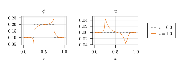
Figure 3. Numerical approximation of $\phi$ and $u$ from (5.1)

In Figure 3 one can see the numerical solution of Algorithm 1 for the initial and terminal time and the corresponding space-time grids are shown in Figure 4.

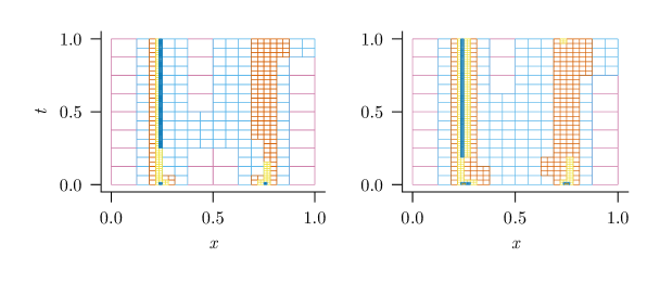
Figure 4. Space-time grids for $\phi$ (left) and $u$ (right) from (5.1)

This highlights the localized behavior of solutions and hence shows the advantage of space-time adaptivity in this context. It also shows the formation of steep gradients in $\phi$ near discontinuities in the initial data.

Next we apply Algorithm 1 to a more realistic problem from geophysics. For the first test, we consider a discontinuous $\phi_{0}$ and $\sigma\equiv 1$ (corresponding to no decompaction weakening). The equations in nondimensional form read

$$\partial_{t}\phi =-(1-\phi)\left(\phi\,u+\frac{1}{60}\partial_{t}u\right),$$ (5.2a)

$$\partial_{t}u =60\,\nabla\cdot(10\,\phi)^{3}(\nabla u+(1-\phi))-\phi\,u,$$ (5.2b)

for $\Omega=(0,3)$ and $T=15.779$, which represent a length of $30\,\mathrm{km}$ and time of $10^{5}\,\mathrm{yr}$ after rescaling.

As discussed in Sections 3.3 and 4.4, we can split the space-time cylinder into time slices whose size solely depends on the continuous problem (via the Lipschitz constant of $\Theta$), but not on the discretization. The corresponding grids for the different slices are concatenated to obtain two separate global space-time grids for $\phi$ and $u$, which are shown in Figure 6; note the localized refinements both in space and in time. Hence we still obtain a space-time adaptive method with the advantage of localized time-steps.

Solving (5.2) for a discontinuous $\phi_{0}$ yields results as depicted in Figure 5 with the associated grids shown in Figure 6.

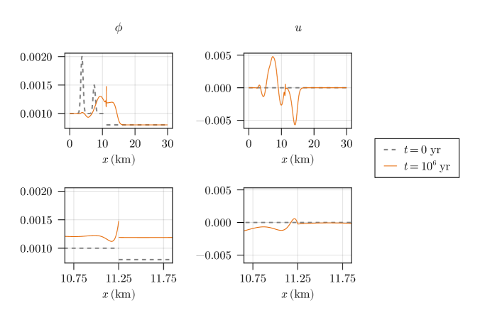
Figure 5. Numerical approximation of $\phi$ and $u$ from (5.2) with zoom-in at the discontinuity (bottom)

Here we plot the numerical solution at the start and after 10 time slices. One can clearly see the similarities with the test problem considered in Figures 1 and 3, for example that discontinuities lead to the formation of steep gradients. This is particularly visible in the bottom of Figure 5, where the solution near the discontinuity is shown. This shows the advantage of our adaptive method in resolving solution features on different scales, which is reflected in the correpsonding grids shown in Figure 6.

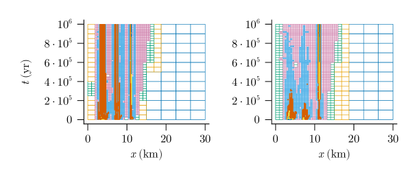
Figure 6. Space-time grids for $\phi$ (left) and $u$ (right) corresponding to Figure 5

The gradients near discontinuities that become increasingly pronounced with time lead to further refinement of the grid near the location of the discontinuity.

Furthermore, we can approximate the solution to the full nonlinear problem with decompaction weakening,

$$\partial_{t}\phi =-(1-\phi)\bigg{(}\frac{\phi^{2}}{\sigma(u)}u+Q\partial_{t}u\bigg{)},$$ (5.3a)

$$\partial_{t}u =\nabla\cdot\phi^{3}\bigg{(}\nabla u+(1-\phi)\begin{pmatrix}0\\ 1\end{pmatrix}\bigg{)}-\frac{\phi^{2}}{\sigma(u)}u,$$ (5.3b)

with $\sigma(u)=1-\tfrac{499}{1000}\left(1+\tanh\left(-\tfrac{1000}{3}u\right)\right)$, $d=2$, $\Omega=(0,1)^{2}$ and $T=10$. In this case, the solution exhibits channel formation as shown in Figure 7.

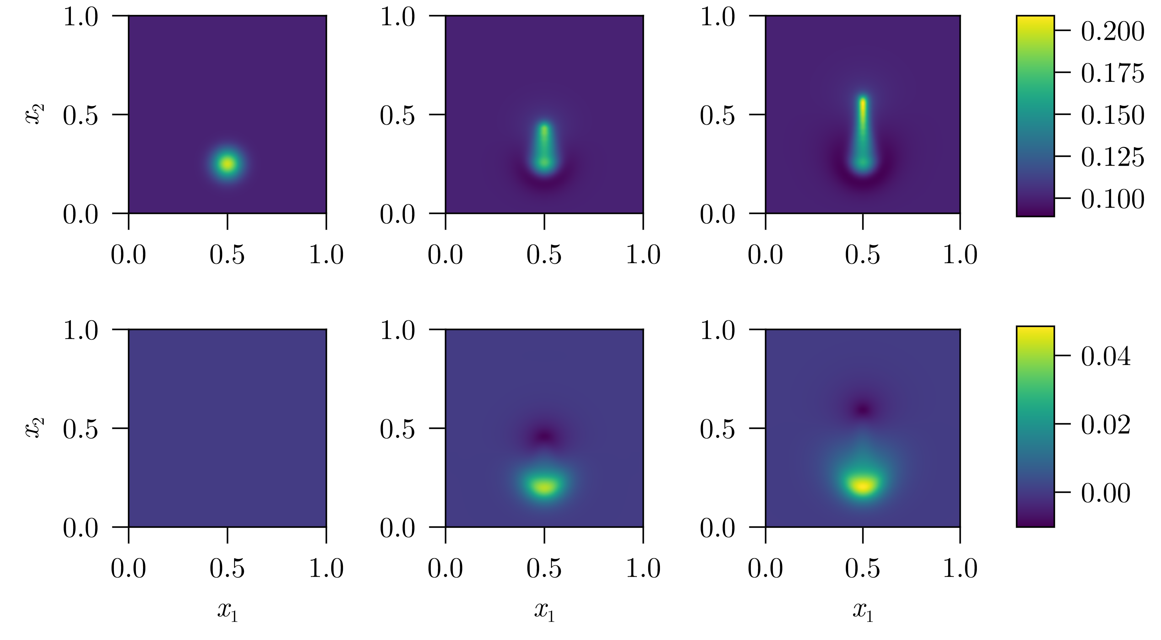
Figure 7. Numerical approximation of $\phi$ (top) and $u$ (bottom) for $t=0,5,10$ (from left to right)

Figure 8 shows the corresponding three-dimensional space-time grids. Here we used 10 time slices and the linearization described in Remark 3.2.

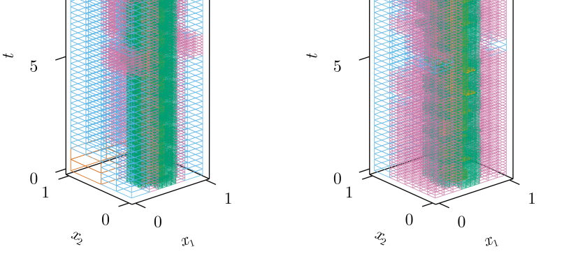
Figure 8. Space-time grids for $\phi$ (left) and $u$ (right) corresponding to Figure 7

5.2. Convergence rates

Using the fully adaptive methods described in Algorithm 2, we now turn to the convergence rates achieved for the test problems considered so far.

We begin with the nonlinear test problem (5.1) and plot the nonlinear error indicators for $\varphi$ and $u$. In Figure 9 one can see the ones for $\varphi$ and in Figure 10 the ones for $u$.

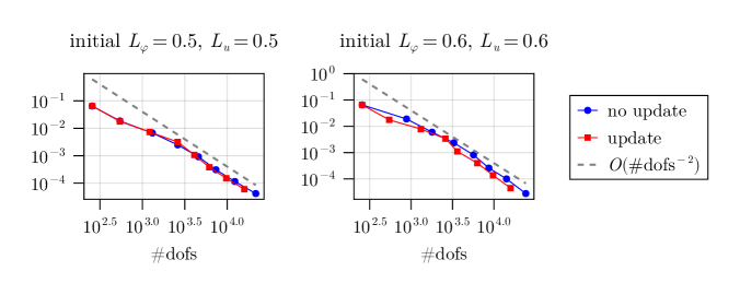
Figure 9. relative $L_{2}$-errors of $\varphi$ for different initial choices of $L_{u}$ and $L_{\varphi}$ corresponding to the solution of (5.1) shown in Figure 3

.

Here we observe that even in the presence of discontinuities, we obtain optimal convergence rates for the $L_{2}(\Omega_{T})$ error of $\varphi$ and the $U$ error of $u$ since we measure 2d-errors and use polynomials of degree 3 to approximate $\varphi$ and $u$. Note that due to the imbedding $U\subseteq L_{2}(0,T;H^{1}(\Omega))\cap H^{1}(0,T;H^{-1}(\Omega))$, we expect a rate of $\frac{3}{2}$ for convergence of the approximation of $u$ in $U$. Furthermore, we observe that the error reduction improves for smaller estimates of Lipschitz constants up to a certain point, but that convergence may be lost if these estimates are chosen too small. This can be avoided by a larger initial Lipschitz constant and adaptively changing it, as it is shown in Figures 10 and 9.

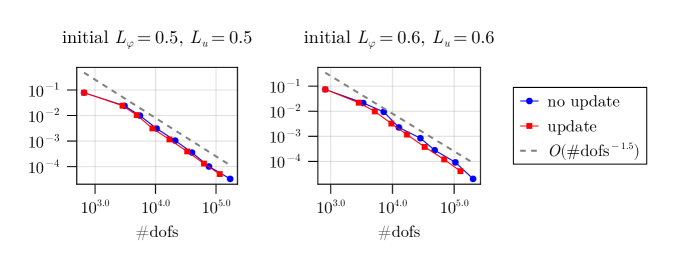
Figure 10. relative $U$-errors of $u$ for different initial choices of $L_{u}$ and $L_{\varphi}$ corresponding to the solution of (5.1) shown in Figure 3

.

We can do the same for the more applied model (5.2). The resulting error plots for discontinuous $\varphi_{0}$ can be found in Figures 12 and 11.

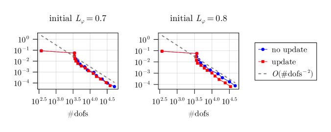
Figure 11. relative $L_{2}$-errors of $\varphi$ for different initial choices of $L_{\varphi}$ corresponding to the solution of (5.2) shown in Figure 5

As in the previous case we observe the expected rates.

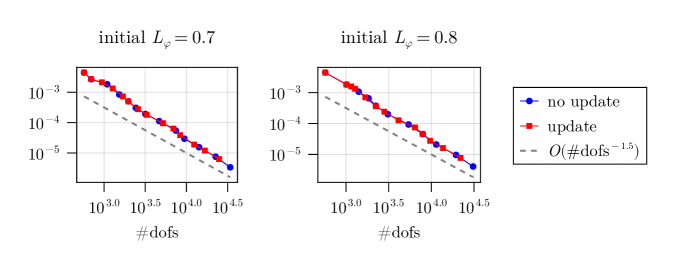
Figure 12. relative $U$-errors of $u$ for different initial choices of $L_{\varphi}$ corresponding to the solution of (5.2) shown in Figure 5

6. Viscous Limit

A common simplification of (2.5) is the viscous limit corresponding to $Q\to 0$, leading to the equations

$$\partial_{t}\varphi =-{\beta(\varphi)}{\kappa(u)},$$ (6.1a)

$$0 =\nabla\cdot\alpha(\varphi)(\nabla u+\zeta(\varphi))-{\beta(\varphi)}{\kappa(u)}.$$ (6.1b)

As before we write (6.1a) in integral form and consider (6.1b) in weak formulation,

$$\varphi(t,\cdot) =\varphi_{0}-\int_{0}^{t}\beta(\varphi)\kappa(u)\,\mathrm{d}s, \text{for $t\in[0,T]$},$$ (6.2a)

$$0 =\nabla\cdot\alpha(\varphi)(\nabla u+\zeta(\varphi))-\beta(\varphi)\kappa(u) \text{in $W^{-1,2}(\Omega)$}.$$ (6.2b)

Furthermore, we assume that Assumptions 1 and 2 are satisfied, leading to similar linearizations as the ones introduced in Section 3. Well-posedness of this approach is shown in [1, Sec. 3].

A space-time adaptive numerical method similar to the one considered above can be obtained along similar lines in this case. Although (6.2b) is elliptic, it is nonetheless time-dependent due to the coupling with $\varphi$. As before, we linearize (6.2b) by means of

$$0=\nabla\cdot\alpha(\varphi)(\nabla u^{(k)}+\zeta(\varphi))-\beta(\varphi)\frac{u^{(k)}}{\sigma(u^{(k-1)})}$$ (6.3)

given the previous iterate $u^{(k-1)}$. Then we define

$$U:=\left\{(u,\eta)\in L_{2}(0,T;H_{0}^{1}(\Omega))\times L_{2}(\Omega_{T})^{d}\,\colon\,\operatorname{div}_{x}\eta\in L_{2}(\Omega_{T})\right\}$$

with the induced graph norm

$$\|(u,\eta)\|_{U}^{2}=\|(u,\eta)\|_{L_{2}(\Omega_{T},\mathbb{R}^{d+1})}^{2}+\|\nabla_{\!x}u\|_{L_{2}(\Omega_{T},\mathbb{R}^{d})}^{2}+\|\operatorname{div}_{x}\eta\|_{L_{2}(\Omega_{T})}^{2}.$$

Next we set $V:=L_{2}(\Omega_{T})\times L_{2}(\Omega_{T},\mathbb{R}^{d})$ with its canonical norm and for each fixed $\overline{u}$ define

$$G[\overline{u}](u,\eta):=\begin{pmatrix}\operatorname{div}_{x}\eta+\beta\,\frac{u}{\sigma(\overline{u})}\\ \eta+\alpha\,\nabla_{\!x}u\end{pmatrix},\quad R:=\begin{pmatrix}0\\ -\alpha\,\zeta\end{pmatrix},$$ (6.4)

This allows us to rewrite (6.3) as

$$G[u^{(k-1)}](u^{(k)},\eta^{(k)})=R.$$ (6.5)

To solve (6.5) numerically for given $\overline{u}$, we compute

$$(u_{\delta},\eta_{\delta})=\operatorname*{arg\,min}_{(v_{\delta},\mu_{\delta})\in U_{\delta}}\|G[\overline{u}](v_{\delta},\mu_{\delta})-R\|_{V}$$

as before. Well-posedness and convergence of the adaptive solver can be shown more easily than above for the general case. In Figure 13, we show a numerical test similar to the one from (5.2) shown in Figure 5, but now with $Q=0$. This time we show the numerical solution at the start and after 15 time slices, and as before we show a detail view near the discontinuity at the bottom of Figure 13.

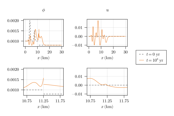
Figure 13. Numerical approximation of $\phi$ and $u$ for discontinuous $\phi_{0}$

The corresponding grids are shown in Figure 14.

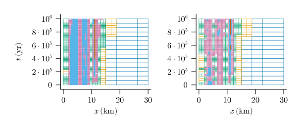
Figure 14. Space-time grids for $\phi$ (left) and $u$ (right) corresponding to Figure 13

Acknowledgements

The authors would like to thank Evangelos Moulas for introducing them to the models discussed in this work and for helpful discussions, Igor Voulis for advice on aspects of the implementation and Henrik Eisenmann for help concerning the results about perturbed fixed-point iterations.

References

- [1] M. Bachmayr, S. Boisserée, and L. M. Kreusser. Analysis of nonlinear poroviscoelastic flows with discontinuous porosities. Nonlinearity, 36:7025–7064, 11 2023.
- [2] V. Barcilon and F. M. Richter. Nonlinear waves in compacting media. Journal of Fluid Mechanics, 164:429–448, 1986.
- [3] P. Binev. Tree approximation for hp-adaptivity. SIAM Journal on Numerical Analysis, 56(6):3346–3357, 2018.
- [4] J. A. D. Connolly and Y. Y. Podladchikov. Compaction-driven fluid flow in viscoelastic rock. Geodinamica Acta, 11(2-3):55–84, 1998.
- [5] A. Costa. Permeability-porosity relationship: A reexamination of the Kozeny-Carman equation based on a fractal pore-space geometry assumption. Geophysical research letters, 33(2), 2006.
- [6] E. DiBenedetto. Degenerate Parabolic Equations. Universitext. Springer New York, 1993.
- [7] T. Führer and M. Karkulik. Space–time least-squares finite elements for parabolic equations. Computers & Mathematics with Applications, 92:27–36, 2021.
- [8] G. Gantner and R. Stevenson. Further results on a space-time FOSLS formulation of parabolic PDEs. ESAIM Math. Model. Numer. Anal., 55(1):283–299, 2021.
- [9] G. Gantner and R. Stevenson. Improved rates for a space-time FOSLS of parabolic PDEs. Numerische Mathematik, 156:133–157, 2024.
- [10] D.G. Luenberger. Optimization by Vector Space Methods. Series in Decision and Control. Wiley, 1969.
- [11] J.C. Mason. Near-best multivariate approximation by fourier series, chebyshev series and chebyshev interpolation. Journal of Approximation Theory, 28(4):349–358, 1980.
- [12] D. McKenzie. The generation and compaction of partially molten rock. Journal of petrology, 25(3):713–765, 1984.
- [13] B. Mößner and U. Reif. Error bounds for polynomial tensor product interpolation. Computing, 86:185–197, 10 2009.
- [14] G. S. Reuber, L. Holbach, and L. Räss. Adjoint-based inversion for porosity in shallow reservoirs using pseudo-transient solvers for non-linear hydro-mechanical processes. Journal of Computational Physics, 423:109797, 2020.
- [15] L. Räss, T. Duretz, and Y. Y. Podladchikov. Resolving hydromechanical coupling in two and three dimensions: spontaneous channelling of porous fluids owing to decompaction weakening. Geophysical Journal International, 218(3):1591–1616, 05 2019.
- [16] L. Räss, N. S. C. Simon, and Y. Y. Podladchikov. Spontaneous formation of fluid escape pipes from subsurface reservoirs. Scientific reports, 8(1):1–11, 2018.
- [17] L. Räss, V. M. Yarushina, N. S.C. Simon, and Y. Y. Podladchikov. Chimneys, channels, pathway flow or water conducting features - an explanation from numerical modelling and implications for co2 storage. Energy Procedia, 63:3761–3774, 2014. 12th International Conference on Greenhouse Gas Control Technologies, GHGT-12.
- [18] I. Utkin and A. Afanasyev. Decompaction weakening as a mechanism of fluid focusing in hydrothermal systems. Journal of Geophysical Research: Solid Earth, 126(9):e2021JB022397, 2021.
- [19] O. V. Vasilyev, Y. Y. Podladchikov, and D. A. Yuen. Modeling of compaction driven flow in poro-viscoelastic medium using adaptive wavelet collocation method. Geophysical Research Letters, 25(17):3239–3242, 1998.
- [20] V. M. Yarushina and Y. Y. Podladchikov. (De)compaction of porous viscoelastoplastic media: Model formulation. Journal of Geophysical Research: Solid Earth, 120(6):4146–4170, 2015.
- [21] V. M. Yarushina, Y. Y. Podladchikov, and J. A. D. Connolly. (De)compaction of porous viscoelastoplastic media: Solitary porosity waves. Journal of Geophysical Research: Solid Earth, 120(7):4843–4862, 2015.
- [22] V. M. Yarushina, Y. Y. Podladchikov, and L. H. Wang. Model for (de)compaction and porosity waves in porous rocks under shear stresses. Journal of Geophysical Research: Solid Earth, 125(8):e2020JB019683, 2020.
- [23] V. M. Yarushina, L. H. Wang, D. Connolly, G. Kocsis, I. Fæstø, S. Polteau, and A. Lakhlifi. Focused fluid-flow structures potentially caused by solitary porosity waves. Geology, 50(2):179–183, 2022.