Bounds on heavy neutral leptons from tree level unitarity

Abstract

Heavy neutral leptons (HNLs) can explain the origin of neutrino masses and oscillations over a wide range of masses. Direct experimental probes of HNLs become unfeasible for masses significantly above the electroweak scale. Consequently, the strongest limits arise from the non-observation of charged lepton flavor-violating processes induced by HNLs at loop level. Counter intuitively, these bounds tighten as the HNL mass increases, an effect that persists within the perturbative regime.

This work explores the precise form of these bounds for HNLs with masses well beyond the electroweak scale by analyzing the full matrix of partial waves (tree-level unitarity). At high energies, the HNL model simplifies to a Yukawa theory, allowing unitarity constraints to be expressed in terms of the total Yukawa coupling $\absolutevalue{Y_{\mathrm{tot}}}^{2}$ involving HNLs, lepton doublets, and the Higgs boson. Processes with $J=0$ and $J=1/2$ yield the well-known bound $\absolutevalue{Y_{\mathrm{tot}}}^{2}\leq 8\pi$. However, the most stringent constraint arises from the eigenvalues of the $(\mathcal{N}^{2}+20)\times(\mathcal{N}^{2}+20)$ matrix, which describes the $J=1$ partial wave amplitude for $\mathcal{N}$ generations of HNLs. This bound is given by $\absolutevalue{Y_{\mathrm{tot}}}^{2}\leq 8\pi/\varphi\approx$15.533$$, where $\varphi$ is the Golden ratio. Finally, we determine the maximum mass that an HNL can have in the type-I seesaw model while remaining the sole source of neutrino masses.

1 Introduction

The discovery of neutrino oscillations remains to this day the only laboratory signal that deviates from Standard Model (SM) predictions Super-Kamiokande:1998kpq ; KamLAND:2003gfh ; SNO:2003bmh . The simplest way to account for neutrino oscillations is by including neutrino mass terms. Many Standard Model extensions accommodate neutrino masses, such as the type I seesaw Minkowski:1977sc ; Yanagida:1979as ; Glashow:1979nm ; Schechter:1981cv and its multiple incarnations Mohapatra:1986bd ; Akhmedov:1995ip , the type II seesaw Cheng:1980qt , type III seesaw Foot:1988aq , loop generated models Zee:1980ai ; Babu:1988ig ; Babu:1988ki ; Ma:2006km , and non-minimal gauge extensions of the SM Gell-Mann:1979vob ; Mohapatra:1979ia .

In this paper, we focus on the type-I seesaw model. This model introduces a set of electrically neutral leptons, $N_{i}$, referred to as Heavy Neutral Leptons (HNLs) also known as sterile neutrinos or right-handed neutrinos to the SM Abdullahi:2022jlv . HNLs interact only through weak-like interactions, additionally suppressed by a small mixing angle $\absolutevalue{\Theta_{\alpha i}}\ll 1$. The minimal number of HNLs that are needed to properly account for neutrino oscillations is two. The addition of these two HNLs can also provide a mechanism for the generation of the asymmetry between matter and antimatter in the universe, and a third, much lighter, HNL can also be a dark matter candidate Asaka:2005an ; Asaka:2005pn ; Boyarsky:2009ix ; Boyarsky:2018tvu ; Klaric:2020phc .

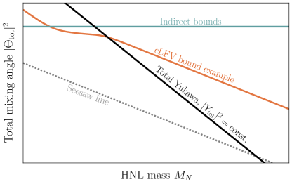
Figure 1: Left: Schematic view of the parameter space of the Type-I seesaw model. Below the dotted line, the heavy neutral leptons do not generate neutrino masses at the observed value. The horizontal line (at masses above the electroweak scale) represents a combined fit to electroweak precision data and charged lepton flavor violation searches Fernandez-Martinez:2016lgt ; Blennow:2023mqx . Corrections to this line appear near the right boundary, where the Yukawa couplings of HNLs are large Urquia-Calderon:2022ufc . Determining the exact position of this boundary is the focus of the current paper. Right: Example of the “HNL penguin” diagram, supressed by the extra powers of the mixing angle $\Theta_{\alpha}$ but growing with the HNL mass. This diagram dominates rates of several cLFV processes Urquia-Calderon:2022ufc and refs. therein.

Collider experiments constrain HNLs with masses below and around the electroweak scale DELPHI:1996qcc ; ATLAS:2015gtp ; CMS:2018jxx ; CMS:2018iaf ; ATLAS:2019kpx ; LHCb:2020wxx ; ATLAS:2022atq ; CMS:2022fut ; CMS:2024xdq ; CMS:2024ake . Collider bounds quickly deteriorate above the electroweak scale ATLAS:2023tkz and one resorts to indirect methods, collectively known as electroweak precision limits Fernandez-Martinez:2016lgt ; Blennow:2023mqx , see Figure 1, left panel. These bounds are dominated by the negative results of searches for charged lepton flavor violation (cLFV) ParticleDataGroup:2024cfk . Within the type-I seesaw model the cLFV processes are mediated by HNLs running in the loops Ilakovac:1994kj ; Illana:2000ic ; Alonso:2012ji ; Chrzaszcz:2019inj . Among all the loop diagrams there is a notable class of “HNL penguins” that exhibit a so-called “non-decoupling" behavior Urquia-Calderon:2022ufc , i.e., the decay width of cLFV processes grows with HNL masses at fixed $\Theta$ Cheng:1991dy ; Tommasini:1995ii ; Urquia-Calderon:2022ufc . Figure 1, right panel shows one such diagram for the processes like $\mu\to eee$ and similar conversion process. These diagrams provide the dominant contribution to the rate at large masses. This seemingly counter-intuitive behavior is actually well-known for theories that undergo spontaneous symmetry breaking (see Chapter 8 of Collins:1984xc and Refs. Collins:1978wz ; DHoker:1984izu ; DHoker:1984mif ; Cheng:1991dy ; Tommasini:1995ii ; Urquia-Calderon:2022ufc ). Particularly in the type I seesaw, this “non-decoupling” is an artifact of keeping the mixing angle fixed while increasing the HNL mass. Such a scaling makes the Yukawa coupling constant grow. Instead, if one increases the mass while keeping the Yukawa fixed, heavy HNLs decouple as expected. The cLFV bounds determine both the upper bound on the mixing angle for a given HNL mass and the maximal value of the mass, as long as the bounds are consistent with perturbativity. Therefore, we have to know the maximal value of Yukawa constants that is consistent with perturbativity.

Given quadratic dependence of the aforementioned corrections on the Yukawa couplings, the exact position of the perturbativity region becomes of great experimental importance.

In this work we determine the actual bounds on heavy HNLs. We do this using the perturbative unitarity framework (for a recent review, see Logan:2022uus ), a now-old tool famously used in the 1970s to provide a first “upper bound” on the Higgs mass Dicus:1973gbw ; Lee:1977eg ; Lee:1977yc . Perturbative unitarity was also used on the top quark before discovery Chanowitz:1978uj ; Chanowitz:1978mv , as well as bounds on non-minimal Higgs sectors Horejsi:2005da ; Hally:2012pu ; Hartling:2014zca , generic Yukawa and vector interactions Allwicher:2021rtd ; Barducci:2023lqx , on effective field theory operators Corbett:2014ora ; Corbett:2017qgl , and many other different models and theories.

The perturbativity bound is usually written in terms of the decay width of HNLs, $\Gamma_{N}$ as $\Gamma_{N}/M_{N}\leq 1/2$, Korner:1992an ; Bernabeu:1993up ; Fajfer:1998px ; Ilakovac:1994kj ; Ilakovac:1999md ; Illana:2000ic ; Abada:2014cca ; Abada:2015oba ; Abada:2016awd ; Abada:2016vzu ; Abada:2023raf . These works refer to Chanowitz:1978mv ; Chanowitz:1978uj for that statement. The latter papers, however, make no claim on the decay width of the additional fermions in question. Other sources in the literature cite different values for this bound Fernandez-Martinez:2015hxa ; Fernandez-Martinez:2016lgt ; Pascoli:2018heg ; Blennow:2023mqx .

Perturbative unitarity is not the only tool we can use to test the perturbativity of the theory; we could also analyze the running of the couplings (the so-called triviality bound) Kuti:1987nr , bounds based on the effects on the running of the Higgs self-coupling to test the vacuum stability Bambhaniya:2016rbb , a multiloop or multiparticle scattering analysis of perturbative unitarity Passarino:1985ax ; Dawson:1988va ; Dawson:1989up ; Durand:1989zs ; Passarino:1990hk ; Durand:1991yf ; Durand:1992wb ; Durand:1993vn ; Maher:1993vj ; Dicus:2004rg ; Dicus:2005ku ; Grinstein:2015rtl .

The lack of a coherent source for the precise value of the perturbativity boundary, along with the need to establish the exact shape of the HNL bounds at large masses, motivated this analysis. The paper is organized as follows: Section 2 reviews the necessary theoretical background, including both perturbative unitarity and type I seesaw theory. Section 3 summarizes all the processes we considered and presents the results on partial waves and the bounds on the Yukawa parameters. Section 4 presents how our results affect current bounds, Section 5 presents the same results at the Seesaw line, which gives us results an “upper bound" on HNL masses. Finally, Section 6 summarizes and concludes the paper.

2 Theoretical preliminaries

2.1 Condition on partial waves

In this section, we re-derive the well-known condition on partial waves (or the amplitude at a specific total angular momentum, $J$) from the unitarity of the $S$ matrix.

Let us begin by considering $2\to 2$ processes. The amplitude, $\mathcal{M}_{if}$ (which is defined from the $S$ matrix: $\matrixelement{f}{S-I}{i}=i(2\pi)^{4}\delta^{4}(p_{i}-p_{f})\mathcal{M}_{if}$), for such processes can be decomposed as a series of partial waves Jacob:1959at

$$\mathcal{M}_{if}(\theta)=16\pi\sum_{J}(2J+1)d_{\mu_{i}\mu_{f}}^{J}(\theta)\,a^{J}_{if}$$ (1)

where $d_{\mu_{i},\mu_{f}}^{J}(\theta)$ are the Wigner $d$-functions (defined in Appendix A), $\mu_{i}=\lambda_{i1}-\lambda_{i2}$ and $\mu_{f}=\lambda_{f1}-\lambda_{f2}$ are the difference of the helicity indices of the incoming and outgoing particles respectively, and $a^{J}_{if}$ are the partial waves.

We can extract the shape of the partial wave if we already have the amplitude

$$a_{if}=\frac{1}{32\pi}\int_{-1}^{1}\differential(\cos\theta)d_{\mu_{i}\mu_{f}}^{J}(\theta)\mathcal{M}_{if}(\theta)\,,$$ (2)

The unitarity condition of the $S$ results in the well-known generalized optical theorem

$$i\left(\mathcal{M}_{fi}^{\ast}-\mathcal{M}_{if}\right)=(2\pi)^{4}\sum_{X}\int\differential\Pi_{X}\,\delta^{4}(p_{i}-p_{X})\mathcal{M}_{iX}\,\mathcal{M}_{fX}^{\ast}\,,$$ (3)

where $\differential\Pi_{X}=\prod_{j}\frac{\differential^{3}p_{j}}{(2\pi)^{3}}\frac{1}{2E_{j}}$ and $X$ sums over single and multi-particle intermediate states. If we restrict the left-hand side of Eq. (3) to $\theta=0$ and the right-hand side up to only include two-particle states in $X$ at very high energies, then we arrive at:

$$\imaginary[a_{if}^{J}]\geq\sum_{H}a_{iH}\,a_{fH}^{\ast}\,,$$ (4)

where $H$ includes any two-particle state. If we only consider elastic scatterings ($i=f$), we arrive at an inequality that is solved in the complex plane. The solutions are

$$\absolutevalue{a_{ii}} \leq 1\,, 0\leq\imaginary[a_{ii}] \leq 1\,, \absolutevalue{\real[a_{ii}]} \leq\frac{1}{2}\,.$$ (5)

Partial waves obey this set of inequalities at all orders of perturbation theory for any complete model. We will consider these inequalities at the lowest order of perturbation theory. As at tree because elastic amplitudes remain real at very high energies, the third inequality in Eq. (5) is the most constraining.

In Section 3 we will deal with different possible processes (both elastic and inelastic) that can form a system that is expressed as a matrix. The best bounds will then come from the biggest eigenvalue of said matrix. This will be elucidated better in Section 3.

2.2 Type I seesaw

In this section, we will review the necessary components of the type I seesaw.

Type I seesaw is an extension to the SM that adds to it $\mathcal{N}$ singlet, neutral fermionic fields, $N_{i,R}$. These are usually known as sterile neutrinos, right-handed neutrinos, or heavy neutral leptons (HNLs). The addition of these fields generates new terms for the SM Lagrangian

$$\mathcal{L}=\mathcal{L}_{\mathrm{SM}}+i\sum_{i}\bar{N}_{i,R}\not{\partial}N_{i,R}-\sum_{\alpha,i}\bar{L}_{\alpha,L}\cdot\tilde{H}\,Y_{\alpha i}N_{i,R}-\frac{1}{2}\sum_{i,j}\bar{N}_{i,R}^{C}\,(M_{M})_{ij}\,N_{j,R}+\mathrm{H.c.}\,,$$ (6)

where $L_{\alpha,L}=\frac{1}{2}(1-\gamma_{5})\,\left(\begin{smallmatrix}\nu_{\alpha}\\ \ell_{\alpha}\end{smallmatrix}\right)$ is the usual SM leptonic doublet, $\tilde{H}=i\sigma_{2}H^{\ast}$ and $H=\left(\begin{smallmatrix}\phi^{+}\\ \phi^{0}\end{smallmatrix}\right)$ is the SM scalar doublet, $Y$ is a Yukawa matrix, $M_{M}$ is the Majorana mass matrix of $N$, and the sums go from $i=1,\dots,\mathcal{N}$ and $\alpha=e,\mu,\tau$.

After spontaneous symmetry breaking, the Yukawa term generates an additional mass term that mixes the $\boldsymbol{\nu}=\left(\begin{smallmatrix}\nu_{e}\\ \nu_{\mu}\\ \nu_{\tau}\end{smallmatrix}\right)$ and the $\boldsymbol{N}=\left(\begin{smallmatrix}N_{1}\\ \vdots\\ N_{\mathcal{N}}\end{smallmatrix}\right)$ fields

$$\mathcal{L}_{\mathrm{mass}}=-\frac{1}{2}\begin{pmatrix}\bar{\boldsymbol{\nu}}_{L}&\bar{\boldsymbol{N}}_{R}^{C}\end{pmatrix}\begin{pmatrix}0&M_{D}\\ M_{D}^{T}&M_{M}\end{pmatrix}\begin{pmatrix}\boldsymbol{\nu}_{L}^{C}\\ \boldsymbol{N}_{R}\end{pmatrix}+\mathrm{H.c.}\,,$$ (7)

where $(M_{D})_{\alpha i}=\frac{v}{\sqrt{2}}Y_{\alpha i}$ and $v$ is the Higgs vacuum expectation value (vev). We can obtain the mass spectrum of the theory by diagonalizing the matrix in Eq. (7). The subsequent diagonalization results in an equation that relates the masses of SM neutrinos, $\boldsymbol{\nu}$, and of our new singlets, $\boldsymbol{N}$. The leading term of this relation is

$$V\,m_{\nu}\,V^{T}\simeq-\Theta M_{N}\Theta^{T}\,,$$ (8)

where $V$ is the PMNS matrix the matrix that diagonalizes the neutrino mass matrix, $\Theta=M_{D}\,M_{N}^{-1}$ is the mixing angle that helps diagonalize the mass matrix and $M_{N}\simeq M_{M}$. The dimensions of $M_{D}$, $\Theta$, and $M_{M}$ depend on the number of singlets we choose to add, but two is the minimal number such that the model can explain neutrino oscillation experiments.

2.2.1 Yukawa term

The equalities detailed above allow us to relate the Yukawa matrix $Y$ with measurable parameters, like $\Theta$ and $M_{N}$:

$$Y_{\alpha i}\simeq\frac{g}{\sqrt{2}M_{W}}\Theta_{\alpha i}(M_{N})_{ii}\,.$$ (9)

We are particularly interested in how large the value of the Yukawa matrix can be such that the unitarity of the $S$ matrix is respected. We shall work in the ultra-high-energy ($\sqrt{s}\gg M_{N},M_{W},M_{Z},M_{H}$) regime where interactions with longitudinal $W$ and $Z$ bosons dominate.

In this energy limit, according to the Goldstone Equivalence theorem, amplitudes with external longitudinal gauge bosons, $W^{\pm}_{L},Z_{L}$, are related to amplitudes with external Goldstone bosons, $\phi^{\pm},\phi_{Z}^{0}$ by Lee:1977eg ; Lee:1977yc ; Chanowitz:1985hj ; Gounaris:1986cr ; Yao:1988aj ; Bagger:1989fc ; Veltman:1989ud ; He:1992nga ; He:1993qa ; He:1993yd ; Denner:1996gb

$$\mathcal{M}(W_{L}^{\pm},Z_{L},\dots)=(i\,C)^{n}\,\mathcal{M}(\phi^{\pm},\phi_{Z}^{0},\dots)+\mathcal{O}\left(M_{W}/\sqrt{s}\right)\,,$$ (10)

where $n$ is the number of external Goldstone bosons. $C$ is a constant related to the renormalization scheme we choose. Since we will only be working with amplitudes at tree-level, we can set $C=1$.

We can thus only consider the interactions that stem from the Yukawa term in Eq. (6).

We can parametrize any Yukawa matrix that follows the seesaw relation in Eq. (8) as

$$Y\simeq i\frac{g}{\sqrt{2}M_{W}}\,V\,\sqrt{m_{\nu}}\,O\,\sqrt{M_{N}}\,,$$ (11)

where $O$ is an arbitrary orthogonal matrix (or semi-orthogonal, in the case we do not have 3 HNLs). This parametrization is called the Casas-Ibarra parametrization Casas:2001sr . We will examine the simplest case, where we only have 2 HNLs with degenerate masses since this is the minimal model that can explain neutrino oscillations. In this case, $O$ can take the shapes

$$O_{\mathrm{NO}} =\begin{pmatrix}0&0\\ \cos\omega&\sin\omega\\ -\sin\omega&\cos\omega\end{pmatrix}\,, O_{\mathrm{IO}}=\begin{pmatrix}\cos\omega&\sin\omega\\ -\sin\omega&\cos\omega\\ 0&0\end{pmatrix}\,,$$ (12)

where the $\mathrm{NO}$ or $\mathrm{IO}$ subscripts indicate whether neutrinos follow the normal or inverted mass hierarchy, respectively.

We can simplify even further. If we want values of $\Theta$ that can be probed by current experiments, then we require $\imaginary(\omega)\gg 1$. Then, we approximate the $O$ matrices as

$$O_{\mathrm{NO}} \approx\frac{e^{-i\omega}}{2}\begin{pmatrix}0&0\\ 1&-i\\ i&1\end{pmatrix}\,, O_{\mathrm{IO}}\approx\frac{e^{-i\omega}}{2}\begin{pmatrix}1&-i\\ i&1\\ 0&0\end{pmatrix}\,.$$ (13)

In this shape, both matrices are rank one. This implies that only one specific linear combination of HNLs interacts with another specific linear combination of the lepton doublet. These linear combinations are

$$N_{R} =\frac{1}{\sqrt{2}}\left(N_{1,R}+iN_{2,R}\right)\,,$$ (14)

$$\nu_{L} =\frac{1}{\sqrt{m_{\nu,i}+m_{\nu,j}}}\left(\sqrt{m_{\nu,j}}\,\nu_{j,L}-i\sqrt{m_{\nu,i}}\,\nu_{i,L}\right)\,,$$ (15)

$$\ell_{L} =\frac{1}{\sqrt{m_{\nu,i}+m_{\nu,j}}}\left(\sqrt{m_{\nu,j}}\,\ell_{j,L}-i\sqrt{m_{\nu,i}}\,\ell_{i,L}\right)\,,$$ (16)

where $L_{i,L}=\sum_{\alpha}\,V_{\alpha i}\,L_{\alpha,L}$, and $(i,j)=(2,3)$ for normal ordering and $(i,j)=(1,2)$ for inverted ordering, and $m_{\nu,1},m_{\nu,2}$ and $m_{\nu,3}$ are the masses of light neutrinos from neutirno oscillation data. Their values are Esteban:2020cvm ; deSalas:2020pgw

$$m_{\nu,2} =$8.61\text{\times}{10}^{-3}\text{\,}\mathrm{e}\mathrm{V}$\,, m_{\nu,3} =$5.01\text{\times}{10}^{-2}\text{\,}\mathrm{e}\mathrm{V}$ \text{for Normal Ordering}\,,$$ (17)

$$m_{\nu,1} =$4.72\text{\times}{10}^{-2}\text{\,}\mathrm{e}\mathrm{V}$\,, m_{\nu,2} =$4.79\text{\times}{10}^{-2}\text{\,}\mathrm{e}\mathrm{V}$ \text{for Inverted Ordering}\,,$$ (18)

In this scenario, the interaction term in Eq. (6) becomes

$$\mathcal{L}_{Y} =-Y_{\mathrm{tot}}\,\bar{L}_{L}\cdot\tilde{H}\,N_{R}+\mathrm{H.c.}\,,$$ (19)

$$=-Y_{\mathrm{tot}}\left[\bar{\nu}_{L}\,N_{R}\,\phi^{0\ast}-\bar{\ell}_{L}\,N_{R}\,\phi^{-}\right]+\mathrm{H.c.}\,,$$

where $Y_{\mathrm{tot}}=\frac{g}{2M_{W}}e^{-i\omega}\sqrt{M_{N}\,(m_{\nu,i}+m_{\nu,j})}$ (notice that $\absolutevalue{Y_{\mathrm{tot}}}^{2}=\sum_{\alpha,i}\absolutevalue{Y_{\alpha i}}^{2}\simeq\frac{g^{2}\,M_{N}\,(m_{\nu,i}+m_{\nu,j})}{4M_{W}^{2}}\,e^{2\imaginary(\omega)}$), and $\phi^{0}=h+i\phi_{Z}^{0}$ where $h$ is the Higgs field and $\phi_{Z}^{0}$ is the Goldstone boson that is eaten by the $Z$ boson.

The reason why we are expressing our Lagrangian in terms of $\phi^{0}$ and not the usual scalar fields ($h$ and $\phi^{0}$) is because $\phi^{0}$ has a defined weak isospin and hypercharge. We can recognize the $\mathrm{SU}(2)\times\mathrm{U}(1)$ structure that the interactions have when working in this basis.

It is straightforward to compute the Feynman Rules of the interactions in Eq. (19). The only caveat comes from the Majorana nature of neutrinos and HNLs. The Majorana nature of both fields gives rise to different Feynman rules from that of usual Dirac particles, but the difference between both is proportional to the masses of HNLs and neutrinos. For our analysis, we can ignore this difference and treat them as Dirac particles, this is the core of the so-called Majorana-Dirac confusion theorem Kayser:1981nw ; Kayser:1982br ; Kayser:1984xc ; Zralek:1997sa .

Some processes we are about to consider receive contributions proportional to the SM gauge couplings and not just our new Yukawa parameters. We neglect them since we are working on the regime where $\absolutevalue{Y_{\mathrm{tot}}}^{2}\sim\mathcal{O}(1)$, which is much bigger than other SM parameters.

The results we will present in Section 3 will only be valid for the cases where $\imaginary(\omega)\gg 1$. This limit should be enough for the probes of current experiments, as none of them can probe smaller values $\imaginary(\omega)$. But for cases where $\imaginary(\omega)\simeq 0$, near the so-called seesaw line, is of academic interest since it gives us an upper bound of HNL masses. We work it out in Section 5.

3 Scattering amplitudes and partial waves

We computed all the amplitudes and partial waves with the help of Mathematica packages FeynCalc 9.3.1 Shtabovenko:2016sxi and FeynArts 3.11 Hahn:2000kx . We obtained the FeynArt amplitudes from a custom-made FeynRules Alloul:2013bka file specifically used for our purposes, which includes the Yukawa interactions we are interested in.

For our analysis, we focus on scattering processes that involve only scalars and fermions. These scatterings are proportional to $\absolutevalue{Y_{\mathrm{tot}}}^{2}$ and correspond to angular momenta of $J=0,\frac{1}{2},1$. The minimal type I seesaw also allows for higher values of $J$ due to interactions between HNLs and the transverse parts of the gauge bosons which we neglect, as they are proportional to the weak coupling constants and the HNL mixing angles.

The angular momentum of each process depends on the initial and final helicities of the particles in the model. We summarize all the processes we will analyze in Table 1. There is also the possibility of having lepton number violating processes (LNV) due to the Majorana nature of HNLs and neutrinos, such as $\ell^{-}\phi^{+}\to\ell^{+}\phi^{-}$, but all such processes are suppressed by $M_{N}^{2}/s$ and are negligibly small for the ultra-high-energy processes we are considering.

		$\mu_{i}=0$			$\mu_{i}=\pm\frac{1}{2}$		$\mu_{i}=\pm 1$
		$++$	$--$	$00$	$+0$	$-0$	$+-$	$-+$
$\mu_{f}=0$	$++$	blue!10$++\to++$	blue!10	blue!10			red!15	red!15
	$--$	blue!10	blue!10$--\to--$	blue!10			red!15	red!15
	$00$	blue!10	blue!10	blue!10			red!15 $+-\to 00$	red!15 $-+\to 00$
$\mu_{f}=\pm\frac{1}{2}$	$+0$				yellow!15 $+0\to+0$	yellow!15
	$-0$				yellow!15	yellow!15 $-0\to-0$
$\mu_{f}=\pm 1$	$+-$	red!15	red!15	red!15 $00\to+-$			red!15 $+-\to+-$	red!15 $-+\to+-$
	$-+$	red!15	red!15	red!15 $00\to-+$			red!15 $+-\to-+$	red!15 $-+\to-+$

Table 1: Table of all possible scatterings with their respective values of angular momentum that can be mediated by $\absolutevalue{Y_{\mathrm{tot}}}^{2}$. It should be noted that the $+$ and $-$ notation is an abbreviation for $+\frac{1}{2}$ and $-\frac{1}{2}$. The processes with the blue background are the processes with $J=0$ angular momentum transferred, the ones in yellow are with $J=\frac{1}{2}$, and the red ones with $J=1$.

3.1 $J=0$ amplitudes

The processes with $J=0$ partial waves are the scatterings of fermions where both initial and final fermions have the same helicities. These processes are

$$N_{\pm}\,\ell_{\pm}^{\pm} \leftrightarrow N_{\pm}\,\ell_{\pm}^{\pm}\,,$$ (20)

$$N_{\pm}\,\nu_{\pm} \leftrightarrow N_{\pm}\,\nu_{\pm}\,,$$ (21)

where the sub-indices denote the helicity of the particle. Of course, at very high energies, we would expect the negatively charged leptons to have negative helicity due to the chiral structure of Yukawa interactions (see Eq. (19)). For neutrinos, since they are Majorana particles, we expect both positive and negative helicities to be able to interact. In the literature, this is usually shown with a symmetrization in the $\nu-N-\phi^{0}$ term in Eq. (19), which we did not show in this instance.

These two scattering processes are due to an $s$ and a $u$ channel. Specifically, the $++\to++$ and the $--\to--$ processes have angular momentum $J=0$, which are due to an $s$ channel. Both channels provides the same bound on the Yukawa couplings because they all have the same partial wave

$$a^{J=0}=-\frac{\absolutevalue{Y_{\mathrm{tot}}}^{2}}{32\pi}\int_{-1}^{1}\differential(\cos\theta)d_{00}^{0}(\theta)=-\frac{Y_{\mathrm{tot}}^{2}}{16\pi}\,,$$ (22)

which the unitarity condition on $S$ gives us

$$\absolutevalue{Y_{\mathrm{tot}}}^{2}\leq 8\pi\,.$$ (23)

What is surprising is that this bound holds independently of the shape of the Yukawa matrix. We present the proof in Appendix B.4.

3.2 $J=\frac{1}{2}$ amplitudes

Scatterings of fermions and scalars are the only processes with partial waves $J=1/2$. In contrast to the $J=0$ scatterings, here we have more possible processes that can be inelastic or elastic. For example, we have a set of elastic scatterings that involve an HNL in the final and initial states

$$N_{\pm}\,\phi_{0}^{+} \leftrightarrow N_{\pm}\,\phi_{0}^{+}\,,$$ (24)

$$N_{\pm}\,\phi_{0}^{0} \leftrightarrow N_{\pm}\,\phi_{0}^{0}\,,$$ (25)

and their respective charge-conjugated processes. Both of these scatterings give the same bounds on the Yukawa coupling. These processes are due to an $s$ and a $u$ channel, but these two do not add one another, as they mediate the process with $N_{+}$ or $N_{-}$ in Eqs. (24) and (25) but not both. The best bounds always come from the $u$ channel

$$a^{J=1/2}=-\frac{\absolutevalue{Y_{\mathrm{tot}}}^{2}}{32\pi}\int_{-1}^{1}\differential(\cos\theta)d_{\frac{1}{2}\frac{1}{2}}^{\frac{1}{2}}(\theta)\sec(\frac{\theta}{2})=-\frac{Y_{\mathrm{tot}}^{2}}{16\pi}\,,$$ (26)

$$\implies\absolutevalue{Y_{\mathrm{tot}}}^{2}\leq 8\pi\,,$$ (27)

the same bound as for $J=0$ scatterings.

We also have scatterings mediated by HNLs that can be elastic or inelastic. We separate two sets of possible scatterings

$$\left\{\begin{aligned} \ell^{-}_{-}\,\phi_{0}^{+}&\leftrightarrow\ell_{-}^{-}\,\phi_{0}^{+}\,,\\ \ell_{-}^{-}\,\phi_{0}^{+}&\leftrightarrow\nu_{-}\,\phi_{0}^{0}\,,\\ \nu_{-}\,\phi_{0}^{0}&\leftrightarrow\nu_{-}\,\phi_{0}^{0}\,,\end{aligned}\right.$$ (28)

$$\left\{\begin{aligned} \nu_{-}\,\phi_{0}^{-}\leftrightarrow\ell_{-}^{-}\,\phi_{0}^{0\ast}\,,\end{aligned}\right.$$ (29)

The processes presented in Eqs. (24) and (25) are both elastic processes, and thus the bound in Eq. (5) apply. But the processes highlighted in Eqs. (28) contain both inelastic and elastic processes, and the one in (29) is completely inelastic, so naively it is not entirely clear how to deal with them. We can extract the necessary information by writing these processes in a matrix. Let’s consider the scatterings in Eq. (28), in the basis $\ell_{-}^{-}\,\phi_{0}^{+},\nu_{-}\,\phi_{0}^{0}$ we have the following partial wave matrix

$$a^{J=1/2}=\frac{Y_{\mathrm{tot}}^{2}}{32\pi}\int_{-1}^{1}\differential(\cos\theta)\,\cos(\frac{\theta}{2})\,d_{\frac{1}{2},\frac{1}{2}}^{\frac{1}{2}}(\theta)\begin{pmatrix}-1&1\\ 1&-1\end{pmatrix}=\frac{\absolutevalue{Y_{\mathrm{tot}}}^{2}}{32\pi}\begin{pmatrix}-1&1\\ 1&-1\end{pmatrix}\,,$$ (30)

the inequalities in Eq. (5) apply to the elements in the diagonal of this matrix, but they also apply to its eigenvalues, and in particular, the strongest bound comes from the biggest eigenvalue. Our labor is then to diagonalize this matrix

$$a^{J=1/2}=\frac{\absolutevalue{Y_{\mathrm{tot}}}^{2}}{32\pi}\begin{pmatrix}-1&1\\ 1&-1\end{pmatrix}\to\frac{\absolutevalue{Y_{\mathrm{tot}}}^{2}}{32\pi}\begin{pmatrix}-2&0\\ 0&0\end{pmatrix}\,,$$ (31)

this eigenvalue corresponds to the scattering $\frac{1}{\sqrt{2}}\left[\ell_{-}^{-}\,\phi_{0}^{+}\,-\,\nu_{-}\,\phi_{0}^{0}\right]\leftrightarrow\frac{1}{\sqrt{2}}\left[\ell_{-}^{-}\,\phi_{0}^{+}\,-\,\nu_{-}\,\phi_{0}^{0}\right]$. Our bound is the same as in Eq. (23).

The same idea applies to the processes in Eq. (29). In the $\nu_{-}\phi_{0}^{-},\ell^{-}_{-}\phi_{0}^{0\ast}$ basis we get the matrix

$$a^{J=1/2}=\frac{\absolutevalue{Y_{\mathrm{tot}}}^{2}}{16\pi}\begin{pmatrix}0&1\\ 1&0\end{pmatrix}\rightarrow\frac{\absolutevalue{Y_{\mathrm{tot}}}^{2}}{16\pi}\begin{pmatrix}1&0\\ 0&-1\end{pmatrix}\,,$$ (32)

which also leads to the bound $\absolutevalue{Y_{\mathrm{tot}}}^{2}\leq 8\pi$.

3.3 $J=1$ amplitudes

Similar to the $J=\frac{1}{2}$, we have different channels, both elastic and inelastic can be written in a matrix like the one in Eq. (31). The processes that contribute to $J=1$ include fermion scatterings $\pm\mp\leftrightarrow\pm\mp$ and $\pm\mp\leftrightarrow\mp\pm$, and scalar-fermion scatterings $\pm\mp\leftrightarrow 00$. This includes the scatterings in we considered for $J=0$ in Eqs. (20) and (21), with the difference that the processes have different helicities

$$N_{\pm}\,\ell^{\mp}_{\mp}\leftrightarrow N_{\pm}\,\ell^{\mp}_{\mp}\,,$$ (33)

$$N_{\pm}\,\nu_{\mp}\leftrightarrow N_{\pm}\,\nu_{\mp}\,,$$ (34)

and also the following set of scatterings

$$\ell^{-}_{-}\,\nu_{+} \leftrightarrow\phi^{-}_{0}\,\phi^{0}_{0}\,,$$ (35)

$$\left\{N_{-}\,N_{+}\,,\nu_{-}\,\nu_{+}\,,\ell^{-}_{-}\,\ell^{+}_{+}\,,\phi^{0}_{0}\,\phi^{0\ast}_{0}\,,\phi^{+}_{0}\,\phi^{-}_{0}\right\} \leftrightarrow\left\{N_{-}\,N_{+}\,,\nu_{-}\,\nu_{+}\,,\ell^{-}_{-}\,\ell^{+}_{+}\,,\phi^{0}_{0}\,\phi^{0\ast}_{0}\,,\phi^{+}_{0}\,\phi^{-}_{0}\right\}\,.$$ (36)

in Eq. (36), every initial state can go into every final state and vice versa.

Both scatterings in Eqs. (33) and (34) give the same partial waves. This fact should not be surprising due to the fact that there is an $\mathrm{SU}(2)$ rotation that relates both amplitudes. The results for both are

$$a^{J=1}=\frac{\absolutevalue{Y_{\mathrm{tot}}}^{2}}{32\pi}\int_{-1}^{1}\differential(\cos\theta)d_{11}^{1}(\theta)=\frac{\absolutevalue{Y_{\mathrm{tot}}}^{2}}{32\pi}\,,$$ (37)

$$\implies\absolutevalue{Y_{\mathrm{tot}}}^{2}\leq 16\pi\,,$$ (38)

which is a weaker result than the ones obtained in previous sections.

For the scatterings in Eqs. (35) in the $\ell_{-}^{-}\,\nu_{+}\,,\phi_{0}^{-}\,\phi_{0}^{0}$ basis we have

$$a^{J=1} =\frac{\absolutevalue{Y_{\mathrm{tot}}}^{2}}{16\sqrt{2}\pi}\begin{pmatrix}0&1\\ 1&0\end{pmatrix}\rightarrow-\frac{\absolutevalue{Y_{\mathrm{tot}}}^{2}}{16\sqrt{2}\pi}\begin{pmatrix}1&0\\ 0&-1\end{pmatrix}\,,$$ (39)

$$\implies\absolutevalue{Y_{\mathrm{tot}}}^{2}\leq 8\sqrt{2}\pi\,,$$ (40)

which is also weaker than every other result by a factor of $\sqrt{2}$.

Finally, the partial wave matrix in Eq. (36) in the $N_{-}\,N_{+}\,,\nu_{-}\,\nu_{+}\,,\ell^{-}_{-}\,\ell^{+}_{+}\,,\phi^{0}_{0}\,\phi^{0\ast}_{0}\,,\phi^{+}_{0}\,\phi^{-}_{0}$ basis reads as

$$a^{J=1} =\frac{\absolutevalue{Y_{\mathrm{tot}}}^{2}}{32\pi}\begin{pmatrix}0&1&1&-\sqrt{2}&-\sqrt{2}\\ 1&0&0&-\sqrt{2}&0\\ 1&0&0&0&-\sqrt{2}\\ -\sqrt{2}&-\sqrt{2}&0&0&0\\ -\sqrt{2}&0&-\sqrt{2}&0&0\\ \end{pmatrix}\rightarrow\frac{\absolutevalue{Y_{\mathrm{tot}}}^{2}}{32\pi}\begin{pmatrix}1+\sqrt{5}&&&&\\ &1-\sqrt{5}&&&\\ &&\sqrt{2}&&\\ &&&-\sqrt{2}&\\ &&&&-2\end{pmatrix}\,,$$ (41)

$$\implies\absolutevalue{Y_{\mathrm{tot}}}^{2}\leq\frac{16\pi}{1+\sqrt{5}}=\frac{8\pi}{\varphi}\,,$$ (42)

where $\varphi=\frac{1+\sqrt{5}}{2}\simeq 1.618\dots$, is the golden ratio. This is the best bound we could find. This bound would correspond to the scattering $\frac{1}{2}\sqrt{\frac{\varphi}{\varphi-\frac{1}{2}}}\left[N_{-}N_{+}+\frac{1}{\varphi}\left(\nu_{-}\nu_{+}+\ell^{-}_{-}\ell^{+}_{+}\right)+\frac{1}{\sqrt{2}}\left(\phi^{+}\phi^{-}+\phi^{0}\phi^{0\ast}\right)\right]\leftrightarrow\frac{1}{2}\sqrt{\frac{\varphi}{\varphi-\frac{1}{2}}}\left[N_{-}N_{+}+\frac{1}{\varphi}\left(\nu_{-}\nu_{+}+\ell^{-}_{-}\ell^{+}_{+}\right)+\frac{1}{\sqrt{2}}\left(\phi^{+}\phi^{-}+\phi^{0}\phi^{0\ast}\right)\right]$.

4 A bound on the bounds

Figure 2: Current bounds on HNL parameters. The colorful bands indicate the bounds from cLFV processes, as allowed by neutrino oscillation data (these values are bounded by a triangular defined by a specific ratio of values of the $\Theta$, see, for example, Section 2 of Tastet:2021vwp ) in the normal (left) and inverted ordering (right). The dark blue shaded region fills the area bounded by EWPD, $|\Theta_{\mathrm{tot}}|^{2}<$5.8\text{\times}{10}^{-4}$$ for NO and $|\Theta_{\mathrm{tot}}|^{2}<$1.2\text{\times}{10}^{-3}$$ for IO Blennow:2023mqx . The black line indicates the line where the unitarity of the $S$ matrix breaks down.

From the relation between the Yukawa coupling and the HNL masses and the $\nu-N$ mixing we have in Eq. (9), then from the perturbative unitarity bounds, we have

$$\absolutevalue{Y_{\mathrm{tot}}}^{2}=\frac{g^{2}\,M_{N}^{2}\,\absolutevalue{\Theta_{\mathrm{tot}}}^{2}}{2\,M_{W}^{2}}=2\sqrt{2}\,G_{F}\,\absolutevalue{\Theta_{\mathrm{tot}}}^{2}M_{N}^{2} \leq\frac{8\pi}{\varphi}\,,$$ (43)

$$\implies\Theta_{\mathrm{tot}}^{2}M_{N}^{2} \lesssim($686.28\text{\,}\mathrm{G}\mathrm{e}\mathrm{V}$)^{2}$$ (44)

where $\Theta_{\mathrm{tot}}^{2}=\sum_{\alpha,i}\absolutevalue{\Theta_{\alpha i}}^{2}$. In terms of Casas-Ibarra parameters, it would translate to

$$\frac{1}{2}\,M_{N}\left(\textstyle\sum_{i}m_{\nu,i}\right)\exp(\imaginary\omega)\lesssim($686.28\text{\,}\mathrm{G}\mathrm{e}\mathrm{V}$)^{2}\,.$$ (45)

We remind the reader that these results are only valid for $\mathrm{Im}\omega\gg 1$, way above the seesaw line, the only region of the parameter space that current experiments can probe.

Experimental constraints have already set limits on $\absolutevalue{\Theta_{\alpha i}}^{2}$, and we would expect them to be smaller than ${10}^{-3}$. These bounds are more relevant for HNLs with masses bigger than $m_{N}\gtrsim$20\text{\,}\mathrm{T}\mathrm{e}\mathrm{V}$$. Current direct searches, like the ones performed at the LHC, cannot produce HNLs that are both this heavy and this feeble interacting. Most of the constraints in this range come from indirect searches, such as searches for lepton flavor violating processes (cLFV), such as $\mu\to e\gamma$ or $\mu\to eee$ decays or muon conversion in a nucleus Ilakovac:1994kj ; Illana:2000ic ; Alonso:2012ji ; Chrzaszcz:2019inj ; Granelli:2022eru ; as well as precise measurements of SM parameters (usually called electroweak precision data or EWPD), Fernandez-Martinez:2016lgt ; Chrzaszcz:2019inj ; Blennow:2023mqx .

cLFV processes are mediated by HNLs at loop level, in particular, for processes like $\mu\to eee$ and muon conversion in a nucleus, the HNL mass does not decouple, which means that their branching ratios grow with mass. What is happening is that these processes are proportional to the Yukawa parameter, which is proportional to HNL masses Cheng:1991dy ; Tommasini:1995ii ; Urquia-Calderon:2022ufc .

In contrast, deviations from EWPD from HNLs occur due to a tree-level effect. This is because adding these extra states makes the PMNS matrix effectively nonunitary. The nonunitary parameters are proportional to $\absolutevalue{\Theta_{\alpha,i}}^{2}$. If the theory contained a large enough Yukawa value, non-decoupling loop correction also contribute to an effective non-unitarity Kniehl:1996bd ; Akhmedov:2013hec ; Fernandez-Martinez:2015hxa .

We can use our results derived in previous sections as an indication as to where bounds from these searches are valid. We show where this happens in Fig. 2. The blue area is the EWPD bounds taken from Blennow:2023mqx . The colorful bands in Fig. 2 are the possible regions where cLFV processes can happen according to neutrino data. Any bound to the right of the black line cannot be reliable, as higher loop-level corrections begin to dominate.

5 Unitarity bound at the seesaw line

As we mentioned at the end of Section 2, all the results in Section 3 are only valid for large values of $\imaginary(\omega)$, where the Yukawa matrix is approximately a rank one matrix. For $\omega\simeq 0$, the Yukawa matrix becomes a rank two matrix, and we can no longer treat the theory as if one HNL interacts only with one lepton bidoublet. Instead, in this case, we have two HNL generations interact with two generations of neutrinos and charged leptons.

The general shape of the partial wave matrices with three different flavors of leptons and $\mathcal{N}$ different HNL generations is in Appendix B. In general, obtaining the eigenvalues in the most general case is not possible to do analytically. We only present some analytic results for the $2+2$ case, which covers all the parameter space of the minimal type I seesaw with only two HNLs.

The easiest case is for $J=0$, where the results of Section 3 are still valid because the general shape of the partial wave matrix is itself a rank one. We explicitly show this fact at the start of Appendix B.4. The change comes when writing the bounds in terms of Casas-Ibarra parameters

$$\absolutevalue{Y_{\mathrm{tot}}}^{2}=\frac{g^{2}}{2M_{W}^{2}}\,M_{N}\,\left(\textstyle\sum_{i}m_{\nu,i}\right)\cosh(2\imaginary\omega)\leq 8\pi\,,$$ (46)

We can also do the $J=\frac{1}{2}$ cases analytically. From Appendix B.4, we find that the partial waves matrices are

$$a^{J=\frac{1}{2}}=\left\{\begin{aligned} &-\frac{1}{16\pi}\,Y\,Y^{\dagger}\,,&&\text{for processes in Eqs.~{}\eqref{eq:j_1/2_process_1} and \eqref{eq:j_1/2_process_2}}\,,\\[8.61108pt] &-\frac{1}{16\pi}\,Y^{\dagger}\,Y\,,&&\text{for processes in Eq.~{}\eqref{eq:j_1/2_process_3}}\,,\end{aligned}\right.$$ (47)

where $Y$ is the Yukawa matrix. For our case, this translates into obtaining the eigenvalues of a $2\times 2$ matrix, which gives us the bounds

$$\frac{g^{2}}{4M_{W}^{2}}M_{N}\left[\left(m_{\nu,i}+m_{\nu,j}\right)\cosh(2\imaginary\omega)\pm\sqrt{(m_{\nu,i}+m_{\nu,j})^{2}\cosh^{2}(\imaginary\omega)-4\,m_{\nu,i}m_{\nu,j}}\right]\leq 8\pi\,.$$ (48)

	$M_{N}<\dots\,\left[$\mathrm{G}\mathrm{e}\mathrm{V}$\right]$
	Normal ordering	Inverted ordering
$J=0$	$1.30\text{\times}{10}^{16}$	$8.01\text{\times}{10}^{15}$
$J=\frac{1}{2}$	$1.52\text{\times}{10}^{16}$	$1.59\text{\times}{10}^{16}$
$J=1$	$9.33\text{\times}{10}^{15}$	$7.60\text{\times}{10}^{15}$

Table 2: Maximum allowed value of the HNL masses depending on the scattering processes considered for each neutrino mass ordering.

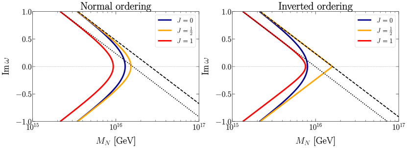
Figure 3: Comparison with the different allowed values of the parameter space, such that tree-level perturbativity is allowed for different values of $\imaginary(\omega)$ and $M_{N}$. The black dashed, and dotted lines are the results obtained in Section 3, whereas the colored lines would be the more exact solution for arbitrary values of $\imaginary(\omega)$ (read the main text for more information). Everything to the left of the lines is allowed by tree-level unitarity.

The case for $J=1$ is much more delicate since the matrix to diagonalize in Eq. (41) becomes a $14\times 14$ matrix that is much harder to obtain analytically.

As we mentioned earlier, our main interest in the generalized case is to obtain the value of the partial waves when $\omega=0$ on the seesaw line. This would give us an “upper bound" on the HNL masses, such that unitarity at tree level is maintained. We can easily obtain analytic solutions for $J=0$ and $J=\frac{1}{2}$; we have to set $\omega=0$ for Eqs. (46) and (48) and solve for $M_{N}$, given a set of neutrino masses. We also provide the results for $J=1$, which we could only obtain numerically. These results are in Table 2, and in Fig. 3 where we compare the more general results with those derived in Section 3.

All of the results agree with the general lore that neutrino masses are generated, at most, around the GUT scale ($\sim${10}^{15}\text{\,}\mathrm{G}\mathrm{e}\mathrm{V}$$) if we want tree-level unitarity to hold Maltoni:2000iq .

6 Summary and conclusions

The addition of heavy neutral leptons is one of the most compelling solutions to the neutrino mass question. This model has an associated lack of predictibility to it, what is the mass of these elusive particles? What is the value of the mixing matrix with SM neutrinos?

The $S$ matrix is unitary for any renormalizable theory. The fact that tree-level compu- tations can violate it indicates a breakdown in perturbation theory. In this work we found the region of the parameter space where the type I seesaw model stops being unitarity. We find that the theory stops being unitary when $\absolutevalue{Y_{\mathrm{tot}}}^{2}\leq 8\pi/\varphi\simeq$15.533$\dots$

Associated with this analysis, we also found the maximal value of the HNL masses that preserves the unitarity of the $S$ matrix and allows the theory to generate neutrino masses. This limit is between $10^{15}-10^{16}\,$\mathrm{G}\mathrm{e}\mathrm{V}$$ for the inverted and normal ordering of neutrino masses, in accordance with the usual lore that “neutrino masses are generated at the GUT scale".

We would also like to state that there is nothing wrong with the values of the theory not satisfying the tree-level unitarity or perturbativity. We can always refine the unitarity bound by doing a one loop analysis on the model, which we would expect would ameliorate the bound Logan:2022uus , or it was suggested by Passarino:1985ax it could refine the bound and restrict the parameter space even more. It is even more unclear the results one would get from two-loops.

Of course, there is nothing wrong with the breakdown of perturbation theory. One of the pillars of the SM, quantum chromodynamics (QCD), violates perturbativity; lattice and several next-to-leading order computations are necessary to generate results that agree with experiments. No one or nothing is telling us that the theory that generates neutrino masses should not be strongly interacting, a possibility seldom discussed in the literature.

A large enough Yukawa coupling would make any amplitude proportional to it unreliable. For cLFV processes, mediated by loop diagrams proportional to Yukawa couplings, further loops might be necessary to give more accurate results. The same idea applies to EWPD, with enough values of Yukawa loop corrections dominate over tree-level ones.

Appendix A Definitions and conventions

In this Appendix we write the definitions and conventions of different important functions.

A.1 Wigner $d$-functions

We collect here some properties and definitions related to Wigner $d$-functions. For a more elaborate discussion, we refer the reader to Chapter 4 of Varshalovich:1988ifq .

The Wigner $D$ functions are defined as matrix elements of the rotation operator $\mathcal{R}(\phi,\theta,\psi)=e^{-i\phi J_{x}}\,e^{-i\theta J_{y}}\,e^{-i\psi J_{z}}$ where $J_{x},J_{y},J_{z}$ are the generators of the $\mathrm{SU}(2)$ group. Then

$$D^{j}_{m^{\prime},m}(\phi,\theta,\psi)\equiv\matrixelement{jm^{\prime}}{\mathcal{R}(\phi,\theta,\psi)}{jm}=e^{-m^{\prime}\phi}d_{m^{\prime},m}^{j}(\theta)e^{-im\psi}\,,$$ (49)

where $j=0,\frac{1}{2},1,\dots$ and $m=-j,-j+1,\dots,j-1,j$. The Wigner (small) $d$-functions are

$$d_{m^{\prime},m}^{j}(\theta)=D^{j}_{m^{\prime},m}(0,\theta,0)=\matrixelement{jm^{\prime}}{e^{-\theta J_{y}}}{jm}\,,$$ (50)

where $d_{m^{\prime},m}^{j}(\theta)$ are real functions that follow

$$\int_{-1}^{1}\differential(\cos\theta)\,d_{m^{\prime},m}^{j}(\theta)\,d_{m^{\prime},m}^{j^{\prime}}(\theta)=\frac{2\,\delta_{jj^{\prime}}}{2j+1}\,,$$ (51)

$$d_{m^{\prime},m}^{j}(\theta)=d_{-m,-m^{\prime}}^{j}=(-1)^{m^{\prime}-m}d_{m,m^{\prime}}^{j}\,.$$ (52)

The explicit expression for some Wigner $d$-functions used for our analysis are

$$d_{0,0}^{0}(\theta) =1\,,$$ (53)

$$d_{\frac{1}{2},\frac{1}{2}}^{\frac{1}{2}}(\theta) =\cos\frac{\theta}{2}\,,$$ (54)

$$d_{01}^{1}(\theta) =-\frac{\sin\theta}{\sqrt{2}}\,,\hskip 28.45274ptd_{11}^{1}(\theta)=\cos^{2}\frac{\theta}{2}\,,$$ (55)

A.2 Spinor helicity formalism

The helicity spinors in the chiral basis are (see Appendix A of Giunti:2007ry )

$$u_{h}(p) =\begin{pmatrix}-\sqrt{E+h\absolutevalue{\vec{p}}}\,\chi_{h}(\hat{p})\\ \sqrt{E-h\absolutevalue{\vec{p}}}\,\chi_{h}(\hat{p})\end{pmatrix}\,, v_{h}(p) =-h\,\begin{pmatrix}\sqrt{E-h\absolutevalue{\vec{p}}}\,\chi_{-h}(\hat{p})\\ \sqrt{E+h\absolutevalue{\vec{p}}}\,\chi_{-h}(\hat{p})\end{pmatrix}\,,$$ (56)

where $h,E$, $\vec{p}$ and $\hat{p}$ are the helicity, energy, three momentum, and direction of three-momentum of the particle in question. The two-component helicity spinors, $\chi_{h}$, are

$$\chi_{+}(\hat{p}) =\begin{pmatrix}\cos\frac{\theta}{2}\\ \sin\frac{\theta}{2}\,e^{i\phi}\end{pmatrix}\,, \chi_{-}(\hat{p}) =\begin{pmatrix}-\sin\frac{\theta}{2}\,e^{-i\phi}\\ \cos\frac{\theta}{2}\end{pmatrix}\,,$$ (57)

where $\theta$ and $\phi$ come from the parametrization of the direction of three momentum

$$\hat{p}(\theta,\phi)=\left(\sin\theta\cos\phi,\sin\theta\sin\phi,\cos\theta\right)\,.$$ (58)

For our case, we were dealing exclusively with $2\to 2$ scatterings with a center of mass energy much larger than any of the masses of the particles. We parametrize the four four-momenta $p_{a}+p_{b}\to p_{1}+p_{2}$ as

$$p_{a} =\frac{\sqrt{s}}{2}\left(1,\hat{p}(0,\phi)\right)\,, p_{b} =\frac{\sqrt{s}}{2}\left(1,\hat{p}(\pi,\phi+\pi)\right)\,,$$ (59)

$$p_{1} =\frac{\sqrt{s}}{2}\left(1,\hat{p}(\theta,\phi)\right)\,, p_{2} =\frac{\sqrt{s}}{2}\left(1,\hat{p}(\pi-\theta,\phi+\pi)\right)\,.$$ (60)

Appendix B Amplitudes and bounds for general Yukawa couplings

In this Appendix, we will present the amplitudes for the different processes we considered. In the main text, we presented the results in simplified cases with an approximate $L$ symmetry, where we effectively only have one HNL interacting with one lepton doublet.

Without making this consideration, the Lagrangian reads as

$$\mathcal{L}_{Y} =-\sum_{\alpha,i}Y_{\alpha i}\left[\bar{\nu}_{\alpha,L}\,N_{i,R}\,\phi^{0\ast}-\bar{\ell}_{\alpha,L}\,N_{i,R}\,\phi^{-}\right]+\mathrm{H.c.}\,,$$ (61)

where $\alpha\in\left(e,\mu,\tau\right)$ and $i=1,\dots,\mathcal{N}$ where $\mathcal{N}$ is the number of HNLs we decided to add to our theory.

The Feynman rules of the interactions in Eq. (61) should be straightforward as well.

In the remaining part of the Appendix, we will present the shape of the amplitudes of all the processes we considered without any assumptions of the particular shape of Yukawa particles and then present the shape of partial waves. The results in the main text are recovered if we substitute the combination of Yukawa couplings by $\absolutevalue{Y_{\mathrm{tot}}}^{2}$.

B.1 $J=0$ amplitudes

The amplitudes for both processes in Eq. (20) and (21) are the same. They are both due to an $s$ channel. Their amplitudes are

$$N_{i}\ell_{\alpha}^{\mp}\to N_{j}\ell_{\beta}^{\mp}:\hskip 28.45274pt\left\{\begin{aligned} --\to--&=-Y_{\alpha i}^{\ast}\,Y_{\beta j}^{\phantom{\ast}}\,,\\ ++\to++&=-Y_{\alpha i}^{\phantom{\ast}}\,Y_{\beta j}^{\ast}\,,\\ \end{aligned}\right.$$ (62)

$$N_{i}\nu_{\alpha}\to N_{j}\nu_{\beta}:\hskip 28.45274pt\left\{\begin{aligned} --\to--&=-Y_{\alpha i}^{\ast}\,Y_{\beta j}^{\phantom{\ast}}\,,\\ ++\to++&=-Y_{\alpha i}^{\phantom{\ast}}\,Y_{\beta j}^{\ast}\,,\\ \end{aligned}\right.$$ (63)

B.2 $J=\frac{1}{2}$ amplitudes

$$N_{i}\phi^{+}\to N_{j}\phi^{+}:\hskip 28.45274pt\left\{\begin{aligned} +0\to+0=-\sum_{\gamma}Y_{\gamma i}^{\phantom{\ast}}\,Y_{\gamma j}^{\ast}\,\sec(\theta/2)\,,\\ -0\to-0=-\sum_{\gamma}Y_{\gamma i}^{\phantom{\ast}}\,Y_{\gamma j}^{\ast}\,\cos(\theta/2)\,,\end{aligned}\right.$$ (64)

$$N_{i}\phi^{0}\to N_{j}\phi^{0}:\hskip 28.45274pt\left\{\begin{aligned} +0\to+0=-\sum_{\gamma}Y_{\gamma i}^{\phantom{\ast}}\,Y_{\gamma j}^{\ast}\,\sec(\theta/2)\,,\\ -0\to-0=-\sum_{\gamma}Y_{\gamma i}^{\phantom{\ast}}\,Y_{\gamma j}^{\ast}\,\cos(\theta/2)\,,\end{aligned}\right.$$ (65)

$$\ell_{\alpha}^{-}\phi^{+}\to\ell_{\beta}^{-}\phi^{+}:\hskip 28.45274pt -0\to-0=-\sum_{k}Y_{\alpha k}^{\ast}\,Y_{\beta k}^{\phantom{\ast}}\,\cos(\theta/2)\,,$$ (66)

$$\ell_{\alpha}^{-}\phi^{+}\to\nu_{\beta}\phi^{0}:\hskip 28.45274pt -0\to-0=\sum_{k}Y_{\alpha k}^{\ast}\,Y_{\beta k}^{\phantom{\ast}}\,\cos(\theta/2)\,,$$ (67)

$$\nu_{\alpha}\phi^{0}\to\nu_{\beta}\phi^{0}:\hskip 28.45274pt -0\to-0=-\sum_{k}Y_{\alpha k}^{\ast}\,Y_{\beta k}^{\phantom{\ast}}\,\cos(\theta/2)\,,$$ (68)

$$\ell_{\alpha}^{-}\phi^{-}\to\ell_{\beta}^{-}\phi^{-}:\hskip 28.45274pt -0\to-0=-\sum_{k}Y_{\alpha k}^{\ast}\,Y_{\beta k}^{\phantom{\ast}}\,\sec(\theta/2)\,,$$ (69)

$$\nu_{\alpha}\phi^{0\ast}\to\nu_{\beta}\phi^{0\ast}:\hskip 28.45274pt -0\to-0=-\sum_{k}Y_{\alpha k}^{\ast}\,Y_{\beta k}^{\phantom{\ast}}\,\sec(\theta/2)\,,$$ (70)

$$\nu_{\alpha}\phi^{-}\to\ell_{\beta}^{-}\phi^{0\ast}:\hskip 28.45274pt -0\to-0=\sum_{k}Y_{\alpha k}^{\ast}\,Y_{\beta k}^{\phantom{\ast}}\,\sec(\theta/2)\,,$$ (71)

B.3 $J=1$ amplitudes

$$N_{i}\ell_{\alpha}^{\mp}\to N_{j}\ell_{\beta}^{\mp}:\hskip 28.45274pt\left\{\begin{aligned} +-\to+-&=Y_{\alpha j}^{\ast}\,Y_{\beta i}^{\phantom{\ast}}\,,\\ -+\to-+&=Y_{\alpha j}^{\phantom{\ast}}\,Y_{\beta i}^{\ast}\,,\\ \end{aligned}\right.$$ (72)

$$N_{i}\nu_{\alpha}\to N_{j}\nu_{\beta}:\hskip 28.45274pt\left\{\begin{aligned} +-\to+-&=Y_{\alpha j}^{\ast}\,Y_{\beta i}^{\phantom{\ast}}\,,\\ -+\to-+&=Y_{\alpha j}^{\phantom{\ast}}\,Y_{\beta i}^{\ast}\,,\\ \end{aligned}\right.$$ (73)

$$\nu_{\alpha}\ell_{\beta}^{-}\to\phi^{0}\phi^{-}:\hskip 28.45274pt\phantom{\{}+-\to 0\,0=-\sum_{k}Y_{\alpha k}^{\phantom{\ast}}\,Y_{\beta k}^{\ast}\cot(\theta/2)\,,$$ (74)

$$N_{i}N_{j}\to\nu_{\alpha}\nu_{\beta}:\hskip 28.45274pt\left\{\begin{aligned} +-\to+-&=Y_{\alpha j}^{\ast}\,Y_{\beta i}^{\phantom{\ast}}\,,\\ -+\to-+&=Y_{\alpha j}^{\phantom{\ast}}\,Y_{\beta i}^{\ast}\,,\\ \end{aligned}\right.$$ (75)

$$N_{i}N_{j}\to\ell_{\alpha}^{\mp}\ell_{\beta}^{\pm}:\hskip 28.45274pt\left\{\begin{aligned} +-\to+-&=Y_{\alpha j}^{\ast}\,Y_{\beta i}^{\phantom{\ast}}\,,\\ -+\to-+&=Y_{\alpha j}^{\phantom{\ast}}\,Y_{\beta i}^{\ast}\,,\\ \end{aligned}\right.$$ (76)

$$N_{i}N_{j}\to\phi^{+}\phi^{-}:\hskip 28.45274pt\phantom{\{}-+\to 0\,0=-\sum_{\gamma}Y_{\gamma i}^{\ast}\,Y_{\gamma j}^{\phantom{\ast}}\,\tan(\theta/2)\,,$$ (77)

$$N_{i}N_{j}\to\phi^{0}\phi^{0\ast}:\hskip 28.45274pt\phantom{\{}-+\to 0\,0=-\sum_{\gamma}Y_{\gamma i}^{\ast}\,Y_{\gamma j}^{\phantom{\ast}}\,\tan(\theta/2)\,,$$ (78)

$$\nu_{\alpha}\nu_{\beta}\to\phi^{0}\phi^{0\ast}:\hskip 28.45274pt\phantom{\{}-+\to 0\,0=-\sum_{k}Y_{\alpha k}^{\ast}\,Y_{\beta k}^{\phantom{\ast}}\,\tan(\theta/2)\,,$$ (79)

$$\ell_{\alpha}^{-}\ell_{\beta}^{+}\to\phi^{+}\phi^{-}:\hskip 28.45274pt\phantom{\{}-+\to 0\,0=-\sum_{k}Y_{\alpha k}^{\ast}\,Y_{\beta k}^{\phantom{\ast}}\,\tan(\theta/2)\,,$$ (80)

B.4 General shape of partial wave matrices

From Eq. (62) and (63), we can derive the $J=0$ partial wave matrix. We have to consider the fact that if we are dealing with three different flavors and $\mathcal{N}$ different HNLs, then our matrix is a $(3+\mathcal{N})$ square matrix.

The partial wave matrix is

$$a^{J=0}=-\frac{1}{16\pi}\begin{pmatrix}\absolutevalue{Y_{e1}^{\phantom{\ast}}}^{2}&Y_{e1}^{\ast}\,Y_{\mu 1}^{\phantom{\ast}}&Y_{e1}^{\ast}\,Y_{\tau 1}^{\phantom{\ast}}&Y_{e1}^{\ast}\,Y_{e2}^{\phantom{\ast}}&\cdots&Y_{e1}^{\ast}\,Y_{\tau\mathcal{N}}^{\phantom{\ast}}\\[6.45831pt] Y_{\mu 1}^{\ast}\,Y_{e1}^{\phantom{\ast}}&\absolutevalue{Y_{\mu 1}^{\phantom{\ast}}}^{2}&Y_{\mu 1}^{\ast}\,Y_{\tau 1}^{\phantom{\ast}}&Y_{\mu 1}^{\ast}\,Y_{e2}^{\phantom{\ast}}&\cdots&Y_{\mu 1}^{\ast}\,Y_{\tau\mathcal{N}}^{\phantom{\ast}}\\[6.45831pt] Y_{\tau 1}^{\ast}\,Y_{e1}^{\phantom{\ast}}&Y_{\tau 1}^{\ast}\,Y_{\mu 1}^{\phantom{\ast}}&\absolutevalue{Y_{\tau 1}^{\phantom{\ast}}}^{2}&Y_{\tau 1}^{\ast}\,Y_{e2}^{\phantom{\ast}}&\cdots&Y_{\tau 1}^{\ast}\,Y_{\tau\mathcal{N}}^{\phantom{\ast}}\\ \vdots&\vdots&\vdots&\vdots&\ddots&\vdots\\ Y_{\tau\mathcal{N}}^{\ast}\,Y_{e1}^{\phantom{\ast}}&Y_{\tau\mathcal{N}}^{\ast}\,Y_{\mu 1}^{\phantom{\ast}}&Y_{\tau\mathcal{N}}^{\ast}\,Y_{\tau 1}^{\phantom{\ast}}&Y_{\tau\mathcal{N}}^{\ast}\,Y_{e2}^{\phantom{\ast}}&\cdots&\absolutevalue{Y_{\tau\mathcal{N}}}^{2}\end{pmatrix}\,.$$ (81)

where the initial (final) states of the columns (rows) are

$$a^{J=0}=\bordermatrix{~{}&N_{1,-}\,e^{-}_{-}&N_{1,-}\,\mu^{-}_{-}&N_{1,-}\,\tau^{-}_{-}&N_{2,-}\,e^{-}_{-}&\cdots&N_{\mathcal{N},-}\,\tau^{-}_{-}\cr N_{1,-}\,e^{-}_{-}\cr N_{1,-}\,\mu^{-}_{-}\cr N_{1,-}\,\tau^{-}_{-}\cr\hfill\vdots\hfill\cr N_{\mathcal{N},-}\,\tau^{-}_{-}}$$ (82)

The unitarity bounds apply to each element in the diagonal individually. In order to obtain the best possible bounds from this process, we would have to obtain the largest eigenvalue in absolute value. Fortunately, it is easy to do. The matrix is a rank-one matrix (meaning it has only one linearly independent row or column), and therefore, we can write it as the product of two vectors

$$a^{J=0}=-\frac{1}{16\pi}\begin{pmatrix}Y_{e1}^{\ast}\\ Y_{\mu 1}^{\ast}\\ \vdots\\ Y_{\tau\mathcal{N}}^{\ast}\end{pmatrix}\begin{pmatrix}Y_{e1}&Y_{\mu 1}\cdots Y_{\tau\mathcal{N}}\end{pmatrix}\,.$$ (83)

Rank-one matrices also have the property of having only one non-zero eigenvalue. Then, we can optimize all bounds by taking the trace

$$a^{J=0}=-\frac{1}{16\pi}\sum_{\alpha,i}\absolutevalue{Y_{\alpha i}}^{2}\,,$$ (84)

$$\implies\sum_{\alpha,i}\absolutevalue{Y_{\alpha i}}^{2}=\absolutevalue{Y_{\mathrm{tot}}}^{2}\leq 8\pi\,,$$

which is exactly the same bounds in Eq. (23). We got this without making any specific assumption on the shape of the Yukawa matrix or the number of additional HNLs.

The fact that the results in the main text hold in the general case is the exception, rather than the rule. For the rest of the processes, we cannot recover the same results as in the main text.

Taking as an example the processes for $J=\frac{1}{2}$ in Eqs. (64) and (65), both give the same $\mathcal{N}\times\mathcal{N}$ matrix. In the $N_{1,+}\phi^{+},N_{2,+}\phi^{+},\dots N_{\mathcal{N}},+\phi^{+}$ basis is

$$a^{J=\frac{1}{2}}=-\frac{1}{16\pi}\sum_{\gamma}\begin{pmatrix}\absolutevalue{Y_{\gamma 1}^{\phantom{\ast}}}^{2}&Y_{\gamma 1}^{\phantom{\ast}}\,Y_{\gamma 2}^{\ast}&\cdots&Y_{\gamma 1}^{\phantom{\ast}}\,Y_{\gamma\mathcal{N}}^{\ast}\\[6.45831pt] Y_{\gamma 2}^{\phantom{\ast}}\,Y_{\gamma 1}^{\ast}&\absolutevalue{Y_{\gamma 2}^{\phantom{\ast}}}^{2}&\cdots&Y_{\gamma 2}^{\phantom{\ast}}\,Y_{\gamma\mathcal{N}}^{\ast}\\[6.45831pt] \vdots&\vdots&\ddots&\vdots\\ Y_{\gamma\mathcal{N}}^{\phantom{\ast}}\,Y_{\gamma 1}^{\ast}&Y_{\gamma\mathcal{N}}^{\phantom{\ast}}\,Y_{\gamma 2}^{\ast}&\cdots&\absolutevalue{Y_{\gamma\mathcal{N}}^{\phantom{\ast}}}^{2}\end{pmatrix}=-\frac{1}{16\pi}Y\,Y^{\dagger}\,.$$ (85)

Here, the matrix does not have a nice and compact shape of its eigenvalues. This matrix is the sum of three rank-one matrices. Therefore, it is at most rank-three and has, at most, three non-zero eigenvalues.

A similar situation arises with the scatterings in Eq. (28) (or the ones in Eqs. (66)–(68)), where we have a $6\times 6$ partial wave matrix.

In the $e^{-}_{-}\,\phi^{+},\mu^{-}_{-}\,\phi^{+},\tau^{-}_{-}\,\phi^{+},\nu_{e,-}^{-}\,\phi^{0},\nu_{\mu,-}^{-}\,\phi^{0},\nu_{\tau,-}^{-}\,\phi^{0}$ the matrix is

$$a^{J=\frac{1}{2}}=\frac{1}{32\pi}\begin{pmatrix}-1&1\\ 1&-1\end{pmatrix}\odot\sum_{k}\begin{pmatrix}\absolutevalue{Y_{ek}^{\phantom{\ast}}}^{2}&Y_{ek}^{\ast}\,Y_{\mu k}^{\phantom{\ast}}&Y_{ek}^{\ast}\,Y_{\tau k}^{\phantom{\ast}}\\[6.45831pt] Y_{\mu k}^{\ast}\,Y_{ek}^{\phantom{\ast}}&\absolutevalue{Y_{\mu k}^{\phantom{\ast}}}^{2}&Y_{\mu k}^{\ast}\,Y_{\tau k}^{\phantom{\ast}}\\[6.45831pt] Y_{\tau k}^{\ast}\,Y_{ek}^{\phantom{\ast}}&Y_{\tau k}^{\ast}\,Y_{\mu k}^{\phantom{\ast}}&\absolutevalue{Y_{\tau k}^{\phantom{\ast}}}^{2}\end{pmatrix}\,,$$ (86)

where $\odot$ denotes the Kronecker product of two matrices. The eigenvalues of the Kronecker product of two matrices are the product of their eigenvalues (see, for example, Chapter 5 of Merris:1997book ). Our problem reduces to get the eigenvalues of

$$a^{J=\frac{1}{2}}=-\frac{1}{16\pi}\sum_{k}\begin{pmatrix}\absolutevalue{Y_{ek}^{\phantom{\ast}}}^{2}&Y_{ek}^{\ast}\,Y_{\mu k}^{\phantom{\ast}}&Y_{ek}^{\ast}\,Y_{\tau k}^{\phantom{\ast}}\\[6.45831pt] Y_{\mu k}^{\ast}\,Y_{ek}^{\phantom{\ast}}&\absolutevalue{Y_{\mu k}^{\phantom{\ast}}}^{2}&Y_{\mu k}^{\ast}\,Y_{\tau k}^{\phantom{\ast}}\\[6.45831pt] Y_{\tau k}^{\ast}\,Y_{ek}^{\phantom{\ast}}&Y_{\tau k}^{\ast}\,Y_{\mu k}^{\phantom{\ast}}&\absolutevalue{Y_{\tau k}^{\phantom{\ast}}}^{2}\end{pmatrix}=-\frac{1}{16\pi}Y^{\dagger}\,Y\,,$$ (87)

which has at most three non-zero eigenvalues. The eigenvalues of an arbitrary Yukawa matrix do not have a compact form.

Finally, as a last example, let us look at the set of scatterings in Eq. (36) (or the scatterings in Eq. (77) – (80)). Here, the shape of the generalized form of Eq. (41) is much more complicated than the ones shown previously in this Appendix.

In a theory with $\mathcal{N}$ HNLs the matrix has dimensions $(\mathcal{N}^{2}+20)\times(\mathcal{N}^{2}+20)$ and is

$$a^{J=1}=\frac{1}{32\pi}\begin{pmatrix}0&\mathbf{Y}&\mathbf{Y}&-\sqrt{2}\,\mathscr{Y}&-\sqrt{2}\,\mathscr{Y}\\ \mathbf{Y}^{\dagger}&0&0&-\sqrt{2}\,\tilde{\mathscr{Y}}&0\\ \mathbf{Y}^{\dagger}&0&0&0&-\sqrt{2}\,\tilde{\mathscr{Y}}\\ -\sqrt{2}\,\mathscr{Y}^{\dagger}&-\sqrt{2}\,\tilde{\mathscr{Y}}^{\dagger}&0&0&0\\ -\sqrt{2}\,\mathscr{Y}^{\dagger}&0&-\sqrt{2}\,\tilde{\mathscr{Y}}^{\dagger}&0&0\end{pmatrix}\,,$$ (88)

where $\mathbf{Y}$ is a matrix of dimension $\mathcal{N}^{2}\times 9$, $\mathscr{Y}$ is a $\mathcal{N}^{2}\times 1$ matrix, and $\tilde{\mathscr{Y}}$ is a $9\times 1$ one. Their shapes are

$$\mathbf{Y}=\begin{pmatrix}\absolutevalue{Y_{e1}^{\phantom{\ast}}}^{2}&Y_{e1}^{\phantom{\ast}}\,Y_{\mu 1}^{\ast}&Y_{e1}^{\phantom{\ast}}\,Y_{\tau 1}^{\ast}&\absolutevalue{Y_{\mu 1}^{\phantom{\ast}}}^{2}&Y_{\mu 1}^{\phantom{\ast}}\,Y_{e1}^{\ast}&Y_{\mu 1}^{\phantom{\ast}}\,Y_{\tau 1}^{\ast}&\absolutevalue{Y_{\tau 1}^{\phantom{\ast}}}^{2}&Y_{\tau 1}^{\phantom{\ast}}\,Y_{e1}^{\ast}&Y_{\tau 1}^{\phantom{\ast}}\,Y_{\mu 1}^{\ast}\\ \vdots&\vdots&\vdots&\vdots&\vdots&\vdots&\vdots&\vdots&\vdots\\ Y_{e\mathcal{N}}^{\phantom{\ast}}\,Y_{e1}^{\ast}&Y_{e\mathcal{N}}^{\phantom{\ast}}\,Y_{\mu 1}^{\ast}&Y_{e\mathcal{N}}^{\phantom{\ast}}\,Y_{\tau 1}^{\ast}&Y_{\mu\mathcal{N}}^{\phantom{\ast}}\,Y_{\mu 1}^{\ast}&\cdots&\cdots&\cdots&\cdots&\cdots\\[4.30554pt] Y_{e1}^{\phantom{\ast}}\,Y_{e2}^{\ast}&Y_{e1}^{\phantom{\ast}}\,Y_{\mu 2}^{\ast}&Y_{e1}^{\phantom{\ast}}\,Y_{\tau 2}^{\ast}&Y_{\mu 1}^{\phantom{\ast}}\,Y_{\mu 2}^{\ast}&\cdots&\cdots&\cdots&\cdots&\cdots\\[4.30554pt] \vdots&\vdots&\vdots&\vdots&\vdots&\vdots&\vdots&\vdots&\vdots\\ \absolutevalue{Y_{e\mathcal{N}}^{\phantom{\ast}}}^{2}&Y_{e\mathcal{N}}^{\phantom{\ast}}\,Y_{\mu\mathcal{N}}^{\ast}&Y_{e\mathcal{N}}^{\phantom{\ast}}\,Y_{\tau\mathcal{N}}^{\ast}&\absolutevalue{Y_{\mu\mathcal{N}}^{\phantom{\ast}}}^{2}&\cdots&\cdots&\cdots&\cdots&\cdots\end{pmatrix}$$ (89)

$$\mathscr{Y} =\sum_{\alpha}\begin{pmatrix}\absolutevalue{Y_{\alpha 1}}^{2}\\ \vdots\\ Y_{\alpha\mathcal{N}}\,Y_{\alpha 1}^{\ast}\\ Y_{\alpha 1}\,Y_{\alpha 2}^{\ast}\\ \vdots\\ \absolutevalue{Y_{\alpha\mathcal{N}}}^{2}\\ \end{pmatrix}\,, \tilde{\mathscr{Y}} =\sum_{i}\begin{pmatrix}\absolutevalue{Y_{ei}}^{2}\\ Y_{\mu i}\,Y_{ei}^{\ast}\\ Y_{\tau i}\,Y_{ei}^{\ast}\\ \absolutevalue{Y_{\mu i}}^{2}\\ Y_{ei}\,Y_{\mu i}^{\ast}\\ Y_{\tau i}\,Y_{\mu i}^{\ast}\\ \absolutevalue{Y_{\tau i}}^{2}\\ Y_{ei}\,Y_{\tau i}^{\ast}\\ Y_{\mu i}\,Y_{\tau i}^{\ast}\\ \end{pmatrix}\,.$$ (90)

The final task would be to obtain the eigenvalues of this matrix. The analytical computation of these eigenvalues is beyond the scope of this paper.

Appendix C Unitarity beyond $s\to\infty$

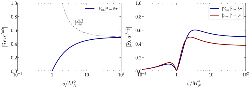
Figure 4: Dependence of the partial waves on $s/M_{N}^{2}$, the gray dashed lines on both plots indicate the upper bound that the partial wave cannot be greater than. On the left, the $J=0$ partial wave changes and the bound (read the text for details). On the right, the $J=\frac{1}{2}$ partial wave changes due to the decay width of the intermediate HNL.

Throughout the main text, we worked only with amplitudes in the ultra-high energy limit, where the center of mass energy, $\sqrt{s}$, is much bigger than any energy scale in the processes considered.

In this Appendix, we will briefly go through the same analysis we did in the main text with a non-negligible HNL mass. We only examine the cases in $J=0$, where we have HNLs in the initial and final states, and the $J=\frac{1}{2}$ processes considered in Eqs. (28), which are much more interesting because we have an intermediate HNL in the $s$ channel which can be in resonance.

For the $J=0$ case, given how we have a massive particle in the final state, the inequality relations on Eq. (5) have to be modified. This is because the integration done in Eq. (3) changes if we have massive particles in the final states. The generalized form of Eq. (5) depends on the three momentum of the final particles, $\absolutevalue{\vec{p}_{f}}$, and is

$$\absolutevalue{a_{ii}} \leq\frac{\sqrt{s}/2}{\absolutevalue{\vec{p}_{f}}}\,, 0\leq\imaginary[a_{ii}] \leq\frac{\sqrt{s}/2}{\absolutevalue{\vec{p}_{f}}}\,, \absolutevalue{\real[a_{ii}]} \leq\frac{1}{2}\,\frac{\sqrt{s}/2}{\absolutevalue{\vec{p}_{f}}}\,.$$ (91)

For all the processes considered in the main text, we have that $\absolutevalue{\vec{p}_{f}}=\sqrt{s}/2$, which is true in the limit where all particles are massless.

If we were to consider the HNL masses for the processes in Eqs. (20) and (21), then $\absolutevalue{\vec{p}_{f}}=\frac{s-M_{N}^{2}}{2\sqrt{s}}$. The amplitudes and the partial waves are also modified to

$$a^{J=0}=- \frac{\absolutevalue{Y_{\mathrm{tot}}}^{2}}{16\pi}\left(\frac{s-M_{N}^{2}}{s}\right)$$

$$\implies \frac{\absolutevalue{Y_{\mathrm{tot}}}^{2}}{16\pi}\left(\frac{s-M_{N}^{2}}{s}\right)\leq\frac{1}{2}\,\frac{s}{s-M_{N}^{2}}\,.$$ (92)

We plot both the left-hand side and the right-hand side of Eq. (92) in Fig. 4 and we find that the bound $\mathrm{\absolutevalue{Y_{\mathrm{tot}}}^{2}}\leq 8\pi$ holds for all energies. We can expect the partial wave of any process with an HNL in the initial or final state to have a similar behavior, and the the best bound would come from $s\to\infty$.

For the $J=\frac{1}{2}$ amplitudes in Eqs. (28), we only included the decay width in the renormalized propagator of the intermediate HNL in the $s$ channel. The decay width is

$$\Gamma_{N}=\frac{\absolutevalue{Y_{\mathrm{tot}}}^{2}}{8\pi}M_{N}\,,$$ (93)

then the partial wave matrix in Eq. (30) gets modified to be

$$a^{J=1/2}= \frac{\absolutevalue{Y_{\mathrm{tot}}}^{2}}{32\pi}\left(\frac{s}{s-M_{N}^{2}+i\Gamma_{N}\,m_{N}^{2}}\right)\begin{pmatrix}-1&1\\ 1&-1\end{pmatrix}\,,$$ (94)

$$\implies \frac{\absolutevalue{Y_{\mathrm{tot}}}^{2}}{16\pi}\absolutevalue{\frac{s(s-M_{N}^{2})}{(s-M_{N}^{2})^{2}+\Gamma_{N}^{2}\,M_{N}^{2}}}\leq\frac{1}{2}\,,$$ (95)

with the decay width in Eq. (93), we have that if we want the inequality to hold for all values of $s$ and $M_{N}^{2}$, then the unitarity bound gets saturated to $\absolutevalue{Y_{\mathrm{tot}}}^{2}\leq 6\,\pi$. We plot the left hand side of Eq. (95) for $\absolutevalue{Y_{\mathrm{tot}}}^{2}=\left\{6\pi,8\pi\right\}$ in Fig. 4.

The case for $J=1$ is much more complicated. After diagonalization, it would be unclear what the final three momentum is, given how we would be dealing with processes where the final particles would have different masses and also different final momentum. Therefore, we will not tackle the problem in this paper.

References

- (1) Super-Kamiokande collaboration, Evidence for oscillation of atmospheric neutrinos, Phys. Rev. Lett. 81 (1998) 1562 [hep-ex/9807003].
- (2) KamLAND collaboration, A High sensitivity search for anti-nu(e)’s from the sun and other sources at KamLAND, Phys. Rev. Lett. 92 (2004) 071301 [hep-ex/0310047].
- (3) SNO collaboration, Measurement of the total active B-8 solar neutrino flux at the Sudbury Neutrino Observatory with enhanced neutral current sensitivity, Phys. Rev. Lett. 92 (2004) 181301 [nucl-ex/0309004].
- (4) P. Minkowski, at a Rate of One Out of Muon Decays?, Phys. Lett. B 67 (1977) 421.
- (5) T. Yanagida, Horizontal gauge symmetry and masses of neutrinos, Conf. Proc. C 7902131 (1979) 95.
- (6) S.L. Glashow, The Future of Elementary Particle Physics, NATO Sci. Ser. B 61 (1980) 687.
- (7) J. Schechter and J.W.F. Valle, Neutrino Decay and Spontaneous Violation of Lepton Number, Phys. Rev. D 25 (1982) 774.
- (8) R.N. Mohapatra and J.W.F. Valle, Neutrino Mass and Baryon Number Nonconservation in Superstring Models, Phys. Rev. D 34 (1986) 1642.
- (9) E.K. Akhmedov, M. Lindner, E. Schnapka and J.W.F. Valle, Left-right symmetry breaking in NJL approach, Phys. Lett. B 368 (1996) 270 [hep-ph/9507275].
- (10) T.P. Cheng and L.-F. Li, Neutrino Masses, Mixings and Oscillations in SU(2) x U(1) Models of Electroweak Interactions, Phys. Rev. D 22 (1980) 2860.
- (11) R. Foot, H. Lew, X.G. He and G.C. Joshi, Seesaw Neutrino Masses Induced by a Triplet of Leptons, Z. Phys. C 44 (1989) 441.
- (12) A. Zee, A Theory of Lepton Number Violation, Neutrino Majorana Mass, and Oscillation, Phys. Lett. B 93 (1980) 389.
- (13) K.S. Babu and E. Ma, Natural Hierarchy of Radiatively Induced Majorana Neutrino Masses, Phys. Rev. Lett. 61 (1988) 674.
- (14) K.S. Babu, Model of ’Calculable’ Majorana Neutrino Masses, Phys. Lett. B 203 (1988) 132.
- (15) E. Ma, Verifiable radiative seesaw mechanism of neutrino mass and dark matter, Phys. Rev. D 73 (2006) 077301 [hep-ph/0601225].
- (16) M. Gell-Mann, P. Ramond and R. Slansky, Complex Spinors and Unified Theories, Conf. Proc. C 790927 (1979) 315 [1306.4669].
- (17) R.N. Mohapatra and G. Senjanovic, Neutrino Mass and Spontaneous Parity Nonconservation, Phys. Rev. Lett. 44 (1980) 912.
- (18) A.M. Abdullahi et al., The present and future status of heavy neutral leptons, J. Phys. G 50 (2023) 020501 [2203.08039].
- (19) T. Asaka, S. Blanchet and M. Shaposhnikov, The nuMSM, dark matter and neutrino masses, Phys. Lett. B 631 (2005) 151 [hep-ph/0503065].
- (20) T. Asaka and M. Shaposhnikov, The MSM, dark matter and baryon asymmetry of the universe, Phys. Lett. B 620 (2005) 17 [hep-ph/0505013].
- (21) A. Boyarsky, O. Ruchayskiy and M. Shaposhnikov, The Role of sterile neutrinos in cosmology and astrophysics, Ann. Rev. Nucl. Part. Sci. 59 (2009) 191 [0901.0011].
- (22) A. Boyarsky, M. Drewes, T. Lasserre, S. Mertens and O. Ruchayskiy, Sterile neutrino Dark Matter, Prog. Part. Nucl. Phys. 104 (2019) 1 [1807.07938].
- (23) J. Klarić, M. Shaposhnikov and I. Timiryasov, Uniting Low-Scale Leptogenesis Mechanisms, Phys. Rev. Lett. 127 (2021) 111802 [2008.13771].
- (24) E. Fernandez-Martinez, J. Hernandez-Garcia and J. Lopez-Pavon, Global constraints on heavy neutrino mixing, JHEP 08 (2016) 033 [1605.08774].
- (25) M. Blennow, E. Fernández-Martínez, J. Hernández-García, J. López-Pavón, X. Marcano and D. Naredo-Tuero, Bounds on lepton non-unitarity and heavy neutrino mixing, JHEP 08 (2023) 030 [2306.01040].
- (26) K.A. Urquía-Calderón, I. Timiryasov and O. Ruchayskiy, Heavy neutral leptons — Advancing into the PeV domain, JHEP 08 (2023) 167 [2206.04540].
- (27) DELPHI collaboration, Search for neutral heavy leptons produced in Z decays, Z. Phys. C 74 (1997) 57.
- (28) ATLAS collaboration, Search for heavy Majorana neutrinos with the ATLAS detector in pp collisions at TeV, JHEP 07 (2015) 162 [1506.06020].
- (29) CMS collaboration, Search for heavy Majorana neutrinos in same-sign dilepton channels in proton-proton collisions at TeV, JHEP 01 (2019) 122 [1806.10905].
- (30) CMS collaboration, Search for heavy neutral leptons in events with three charged leptons in proton-proton collisions at 13 TeV, Phys. Rev. Lett. 120 (2018) 221801 [1802.02965].
- (31) ATLAS collaboration, Search for heavy neutral leptons in decays of bosons produced in 13 TeV collisions using prompt and displaced signatures with the ATLAS detector, JHEP 10 (2019) 265 [1905.09787].
- (32) LHCb collaboration, Search for heavy neutral leptons in decays, Eur. Phys. J. C 81 (2021) 248 [2011.05263].
- (33) ATLAS collaboration, Search for Heavy Neutral Leptons in Decays of W Bosons Using a Dilepton Displaced Vertex in s=13 TeV pp Collisions with the ATLAS Detector, Phys. Rev. Lett. 131 (2023) 061803 [2204.11988].
- (34) CMS collaboration, Search for long-lived heavy neutral leptons with displaced vertices in proton-proton collisions at =13 TeV, JHEP 07 (2022) 081 [2201.05578].
- (35) CMS collaboration, Search for heavy neutral leptons in final states with electrons, muons, and hadronically decaying tau leptons in proton-proton collisions at =13 TeV, 2403.00100.
- (36) CMS collaboration, Search for long-lived heavy neutral leptons decaying in the CMS muon detectors in proton-proton collisions at = 13 TeV, 2402.18658.
- (37) ATLAS collaboration, Search for Majorana neutrinos in same-sign WW scattering events from pp collisions at TeV, Eur. Phys. J. C 83 (2023) 824 [2305.14931].
- (38) Particle Data Group collaboration, Review of particle physics, Phys. Rev. D 110 (2024) 030001.
- (39) A. Ilakovac and A. Pilaftsis, Flavor violating charged lepton decays in seesaw-type models, Nucl. Phys. B 437 (1995) 491 [hep-ph/9403398].
- (40) J.I. Illana and T. Riemann, Charged lepton flavor violation from massive neutrinos in Z decays, Phys. Rev. D 63 (2001) 053004 [hep-ph/0010193].
- (41) R. Alonso, M. Dhen, M.B. Gavela and T. Hambye, Muon conversion to electron in nuclei in type-I seesaw models, JHEP 01 (2013) 118 [1209.2679].
- (42) M. Chrzaszcz, M. Drewes, T.E. Gonzalo, J. Harz, S. Krishnamurthy and C. Weniger, A frequentist analysis of three right-handed neutrinos with GAMBIT, Eur. Phys. J. C 80 (2020) 569 [1908.02302].
- (43) T.P. Cheng and L.-F. Li, Effects of Superheavy Neutrinos in Low-Energy Weak Processes, Phys. Rev. D 44 (1991) 1502.
- (44) D. Tommasini, G. Barenboim, J. Bernabeu and C. Jarlskog, Nondecoupling of heavy neutrinos and lepton flavor violation, Nucl. Phys. B 444 (1995) 451 [hep-ph/9503228].
- (45) J.C. Collins, Renormalization, vol. 26 of Cambridge Monographs on Mathematical Physics, Cambridge University Press, Cambridge (7, 2023), 10.1017/9781009401807.
- (46) J.C. Collins, F. Wilczek and A. Zee, Low-Energy Manifestations of Heavy Particles: Application to the Neutral Current, Phys. Rev. D 18 (1978) 242.
- (47) E. D’Hoker and E. Farhi, Decoupling a Fermion Whose Mass Is Generated by a Yukawa Coupling: The General Case, Nucl. Phys. B 248 (1984) 59.
- (48) E. D’Hoker and E. Farhi, Decoupling a Fermion in the Standard Electroweak Theory, Nucl. Phys. B 248 (1984) 77.
- (49) H.E. Logan, Lectures on perturbative unitarity and decoupling in Higgs physics, 2207.01064.
- (50) D.A. Dicus and V.S. Mathur, Upper bounds on the values of masses in unified gauge theories, Phys. Rev. D 7 (1973) 3111.
- (51) B.W. Lee, C. Quigg and H.B. Thacker, Weak Interactions at Very High-Energies: The Role of the Higgs Boson Mass, Phys. Rev. D 16 (1977) 1519.
- (52) B.W. Lee, C. Quigg and H.B. Thacker, The Strength of Weak Interactions at Very High-Energies and the Higgs Boson Mass, Phys. Rev. Lett. 38 (1977) 883.
- (53) M.S. Chanowitz, M.A. Furman and I. Hinchliffe, Weak Interactions of Ultraheavy Fermions, Phys. Lett. B 78 (1978) 285.
- (54) M.S. Chanowitz, M.A. Furman and I. Hinchliffe, Weak Interactions of Ultraheavy Fermions. 2., Nucl. Phys. B 153 (1979) 402.
- (55) J. Horejsi and M. Kladiva, Tree-unitarity bounds for THDM Higgs masses revisited, Eur. Phys. J. C 46 (2006) 81 [hep-ph/0510154].
- (56) K. Hally, H.E. Logan and T. Pilkington, Constraints on large scalar multiplets from perturbative unitarity, Phys. Rev. D 85 (2012) 095017 [1202.5073].
- (57) K. Hartling, K. Kumar and H.E. Logan, The decoupling limit in the Georgi-Machacek model, Phys. Rev. D 90 (2014) 015007 [1404.2640].
- (58) L. Allwicher, P. Arnan, D. Barducci and M. Nardecchia, Perturbative unitarity constraints on generic Yukawa interactions, JHEP 10 (2021) 129 [2108.00013].
- (59) D. Barducci, M. Nardecchia and C. Toni, Perturbative unitarity constraints on generic vector interactions, JHEP 09 (2023) 134 [2306.11533].
- (60) T. Corbett, O.J.P. Éboli and M.C. Gonzalez-Garcia, Unitarity Constraints on Dimension-Six Operators, Phys. Rev. D 91 (2015) 035014 [1411.5026].
- (61) T. Corbett, O.J.P. Éboli and M.C. Gonzalez-Garcia, Unitarity Constraints on Dimension-six Operators II: Including Fermionic Operators, Phys. Rev. D 96 (2017) 035006 [1705.09294].
- (62) J.G. Korner, A. Pilaftsis and K. Schilcher, Leptonic flavor changing Z0 decays in SU(2) x U(1) theories with right-handed neutrinos, Phys. Lett. B 300 (1993) 381 [hep-ph/9301290].
- (63) J. Bernabeu, J.G. Korner, A. Pilaftsis and K. Schilcher, Universality breaking effects in leptonic Z decays, Phys. Rev. Lett. 71 (1993) 2695 [hep-ph/9307295].
- (64) S. Fajfer and A. Ilakovac, Lepton flavor violation in light hadron decays, Phys. Rev. D 57 (1998) 4219.
- (65) A. Ilakovac, Lepton flavor violation in the standard model extended by heavy singlet Dirac neutrinos, Phys. Rev. D 62 (2000) 036010 [hep-ph/9910213].
- (66) A. Abada, V. De Romeri, S. Monteil, J. Orloff and A.M. Teixeira, Indirect searches for sterile neutrinos at a high-luminosity Z-factory, JHEP 04 (2015) 051 [1412.6322].
- (67) A. Abada, V. De Romeri and A.M. Teixeira, Impact of sterile neutrinos on nuclear-assisted cLFV processes, JHEP 02 (2016) 083 [1510.06657].
- (68) A. Abada and T. Toma, Electron electric dipole moment in Inverse Seesaw models, JHEP 08 (2016) 079 [1605.07643].
- (69) A. Abada, V. De Romeri, J. Orloff and A.M. Teixeira, In-flight cLFV conversion: , and in minimal extensions of the standard model with sterile fermions, Eur. Phys. J. C 77 (2017) 304 [1612.05548].
- (70) A. Abada, J. Kriewald, E. Pinsard, S. Rosauro-Alcaraz and A.M. Teixeira, Heavy neutral lepton corrections to SM boson decays: lepton flavour universality violation in low-scale seesaw realisations, Eur. Phys. J. C 84 (2024) 149 [2307.02558].
- (71) E. Fernandez-Martinez, J. Hernandez-Garcia, J. Lopez-Pavon and M. Lucente, Loop level constraints on Seesaw neutrino mixing, JHEP 10 (2015) 130 [1508.03051].
- (72) S. Pascoli, R. Ruiz and C. Weiland, Heavy neutrinos with dynamic jet vetoes: multilepton searches at , 27, and 100 TeV, JHEP 06 (2019) 049 [1812.08750].
- (73) J. Kuti, L. Lin and Y. Shen, Upper Bound on the Higgs Mass in the Standard Model, Phys. Rev. Lett. 61 (1988) 678.
- (74) G. Bambhaniya, P.S. Bhupal Dev, S. Goswami, S. Khan and W. Rodejohann, Naturalness, Vacuum Stability and Leptogenesis in the Minimal Seesaw Model, Phys. Rev. D 95 (2017) 095016 [1611.03827].
- (75) G. Passarino, Large Masses, Unitarity and One Loop Corrections, Phys. Lett. B 156 (1985) 231.
- (76) S. Dawson and S. Willenbrock, UNITARITY CONSTRAINTS ON HEAVY HIGGS BOSONS, Phys. Rev. Lett. 62 (1989) 1232.
- (77) S. Dawson and S. Willenbrock, RADIATIVE CORRECTIONS TO LONGITUDINAL VECTOR BOSON SCATTERING, Phys. Rev. D 40 (1989) 2880.
- (78) L. Durand, J.M. Johnson and J.L. Lopez, Perturbative Unitarity Revisited: A New Upper Bound on the Higgs Boson Mass, Phys. Rev. Lett. 64 (1990) 1215.
- (79) G. Passarino, W W scattering and perturbative unitarity, Nucl. Phys. B 343 (1990) 31.
- (80) L. Durand, J.M. Johnson and P.N. Maher, Implications of unitarity for low-energy W(l)+-, Z(L) scattering, Phys. Rev. D 44 (1991) 127.
- (81) L. Durand, J.M. Johnson and J.L. Lopez, Perturbative unitarity and high-energy W(L)+-, Z(L), H scattering. One loop corrections and the Higgs boson coupling, Phys. Rev. D 45 (1992) 3112.
- (82) L. Durand, P.N. Maher and K. Riesselmann, Two loop unitarity constraints on the Higgs boson coupling, Phys. Rev. D 48 (1993) 1084 [hep-ph/9303234].
- (83) P.N. Maher, L. Durand and K. Riesselmann, Two loop renormalization constants and high-energy 2 — 2 scattering amplitudes in the Higgs sector of the Standard Model, Phys. Rev. D 48 (1993) 1061 [hep-ph/9303233].
- (84) D.A. Dicus and H.-J. He, Scales of fermion mass generation and electroweak symmetry breaking, Phys. Rev. D 71 (2005) 093009 [hep-ph/0409131].
- (85) D.A. Dicus and H.-J. He, Scales of mass generation for quarks, leptons and majorana neutrinos, Phys. Rev. Lett. 94 (2005) 221802 [hep-ph/0502178].
- (86) B. Grinstein, C.W. Murphy and P. Uttayarat, One-loop corrections to the perturbative unitarity bounds in the CP-conserving two-Higgs doublet model with a softly broken symmetry, JHEP 06 (2016) 070 [1512.04567].
- (87) M. Jacob and G.C. Wick, On the General Theory of Collisions for Particles with Spin, Annals Phys. 7 (1959) 404.
- (88) M.S. Chanowitz and M.K. Gaillard, The TeV Physics of Strongly Interacting W’s and Z’s, Nucl. Phys. B 261 (1985) 379.
- (89) G.J. Gounaris, R. Kogerler and H. Neufeld, Relationship Between Longitudinally Polarized Vector Bosons and their Unphysical Scalar Partners, Phys. Rev. D 34 (1986) 3257.
- (90) Y.-P. Yao and C.P. Yuan, Modification of the Equivalence Theorem Due to Loop Corrections, Phys. Rev. D 38 (1988) 2237.
- (91) J. Bagger and C. Schmidt, Equivalence Theorem Redux, Phys. Rev. D 41 (1990) 264.
- (92) H.G.J. Veltman, The Equivalence Theorem, Phys. Rev. D 41 (1990) 2294.
- (93) H.-J. He, Y.-P. Kuang and X.-y. Li, On the precise formulation of equivalence theorem, Phys. Rev. Lett. 69 (1992) 2619.
- (94) H.-J. He, Y.-P. Kuang and X.-y. Li, Proof of the equivalence theorem in the chiral Lagrangian formalism, Phys. Lett. B 329 (1994) 278 [hep-ph/9403283].
- (95) H.-J. He, Y.-P. Kuang and X.-y. Li, Further investigation on the precise formulation of the equivalence theorem, Phys. Rev. D 49 (1994) 4842.
- (96) A. Denner and S. Dittmaier, Dyson summation without violating Ward identities and the Goldstone boson equivalence theorem, Phys. Rev. D 54 (1996) 4499 [hep-ph/9603341].
- (97) J.A. Casas and A. Ibarra, Oscillating neutrinos and , Nucl. Phys. B 618 (2001) 171 [hep-ph/0103065].
- (98) I. Esteban, M.C. Gonzalez-Garcia, M. Maltoni, T. Schwetz and A. Zhou, The fate of hints: updated global analysis of three-flavor neutrino oscillations, JHEP 09 (2020) 178 [2007.14792].
- (99) P.F. de Salas, D.V. Forero, S. Gariazzo, P. Martínez-Miravé, O. Mena, C.A. Ternes et al., 2020 global reassessment of the neutrino oscillation picture, JHEP 02 (2021) 071 [2006.11237].
- (100) B. Kayser and R.E. Shrock, Distinguishing Between Dirac and Majorana Neutrinos in Neutral Current Reactions, Phys. Lett. B 112 (1982) 137.
- (101) B. Kayser, Majorana Neutrinos and their Electromagnetic Properties, Phys. Rev. D 26 (1982) 1662.
- (102) B. Kayser, Majorana neutrinos, Comments Nucl. Part. Phys. 14 (1985) 69.
- (103) M. Zralek, On the possibilities of distinguishing Dirac from Majorana neutrinos, Acta Phys. Polon. B 28 (1997) 2225 [hep-ph/9711506].
- (104) V. Shtabovenko, R. Mertig and F. Orellana, New Developments in FeynCalc 9.0, Comput. Phys. Commun. 207 (2016) 432 [1601.01167].
- (105) T. Hahn, Generating Feynman diagrams and amplitudes with FeynArts 3, Comput. Phys. Commun. 140 (2001) 418 [hep-ph/0012260].
- (106) A. Alloul, N.D. Christensen, C. Degrande, C. Duhr and B. Fuks, FeynRules 2.0 - A complete toolbox for tree-level phenomenology, Comput. Phys. Commun. 185 (2014) 2250 [1310.1921].
- (107) J.-L. Tastet, O. Ruchayskiy and I. Timiryasov, Reinterpreting the ATLAS bounds on heavy neutral leptons in a realistic neutrino oscillation model, JHEP 12 (2021) 182 [2107.12980].
- (108) A. Granelli, J. Klarić and S.T. Petcov, Tests of low-scale leptogenesis in charged lepton flavour violation experiments, Phys. Lett. B 837 (2023) 137643 [2206.04342].
- (109) B.A. Kniehl and A. Pilaftsis, Mixing renormalization in Majorana neutrino theories, Nucl. Phys. B 474 (1996) 286 [hep-ph/9601390].
- (110) E. Akhmedov, A. Kartavtsev, M. Lindner, L. Michaels and J. Smirnov, Improving Electro-Weak Fits with TeV-scale Sterile Neutrinos, JHEP 05 (2013) 081 [1302.1872].
- (111) F. Maltoni, J.M. Niczyporuk and S. Willenbrock, Upper bound on the scale of Majorana neutrino mass generation, Phys. Rev. Lett. 86 (2001) 212 [hep-ph/0006358].
- (112) D.A. Varshalovich, A.N. Moskalev and V.K. Khersonskii, Quantum Theory of Angular Momentum: Irreducible Tensors, Spherical Harmonics, Vector Coupling Coefficients, 3nj Symbols, World Scientific Publishing Company (1988), 10.1142/0270.
- (113) C. Giunti and C.W. Kim, Fundamentals of Neutrino Physics and Astrophysics, Oxford University Press (2007).
- (114) R. Merris, Multilinear algebra, Gordon and Breach Science Publishers (1997).