PointSAM: Pointly-Supervised Segment Anything Model for Remote Sensing Images

Abstract

Segment Anything Model (SAM) is an advanced foundational model for image segmentation, widely applied to remote sensing images (RSIs). Due to the domain gap between RSIs and natural images, traditional methods typically use SAM as a source pre-trained model and fine-tune it with fully supervised masks. Unlike these methods, our work focuses on fine-tuning SAM using more convenient and challenging point annotations. Leveraging SAM’s zero-shot capabilities, we adopt a self-training framework that iteratively generates pseudo-labels for training. However, if the pseudo-labels contain noisy labels, there is a risk of error accumulation. To address this issue, we extract target prototypes from the target dataset and use the Hungarian algorithm to match them with prediction prototypes, preventing the model from learning in the wrong direction. Additionally, due to the complex backgrounds and dense distribution of objects in RSI, using point prompts may result in multiple objects being recognized as one. To solve this problem, we propose a negative prompt calibration method based on the non-overlapping nature of instance masks. In brief, we use the prompts of overlapping masks as corresponding negative signals, resulting in refined masks. Combining the above methods, we propose a novel Pointly-supervised Segment Anything Model named PointSAM. We conduct experiments on RSI datasets, including WHU, HRSID, and NWPU VHR-10, and the results show that our method significantly outperforms direct testing with SAM, SAM2, and other comparison methods. Furthermore, we introduce PointSAM as a point-to-box converter and achieve encouraging results, suggesting that this method can be extended to other point-supervised tasks. The code is available at https://github.com/Lans1ng/PointSAM.

I Introduction

Foundation models are versatile, large-scale models designed for a wide range of tasks and applications. They have demonstrated exceptional performance in areas such as natural language processing (e.g., BERT[1] and GPT-3[2]) and multimodal tasks (e.g., CLIP[3] and ALIGN [4]). Recently, the Segment Anything Model (SAM) [5, 6] was introduced as a foundation model specifically for image segmentation. Trained on a billion-scale dataset of masks and prompts, SAM can be applied to various downstream tasks requiring promptable segmentation, including healthcare [7, 8], autonomous driving [9], and remote sensing [10, 11, 12].

Despite SAM’s strong zero-shot capabilities, challenges persist in handling out-of-distribution (OOD) data and domain shifts in remote sensing images (RSIs). Many categories in RSIs are not represented in SAM’s training data, and RSIs, typically captured from aerial or satellite perspectives, differ significantly from natural images. Consequently, recent studies [10, 13, 14, 15] have focused on fine-tuning SAM for specific tasks. For example, RS-Prompter [10] uses queries or anchors as prompts to guide SAM’s mask decoder for instance segmentation. Similarly, SAM-CD [13] employs FastSAM’s encoder and introduces adapters for fine-tuning in change detection tasks.

Figure 1: (a) Training pipeline of vanilla SAM. (b) Training pipeline of self-training based pointly-supervised SAM. Sup. means supervise.

While these methods have shown promising results, they also require full mask annotations, which are difficult and time-consuming to obtain. As a result, some approaches [16, 17, 18] have begun exploring label-efficient strategies for SAM. WeSAM[16] and SlotSAM[18] leverage self-training techniques [19] with weak labels, such as points, boxes, and polygons, to generate pseudo-labels, allowing the network to predict complete masks. Cat-SAM [17] adopts a few-shot learning approach to fine-tune SAM using box prompts to predict masks. While using boxes or coarse masks as prompts have yielded excellent results, point annotations remain less effective than fully supervised methods. Moreover, point annotations are much cheaper than masks and boxes , particularly for RSIs with numerous dense objects. Therefore, this paper aims to fine-tune SAM for RSIs using the most challenging yet cost-effective point annotations.

As shown in Fig. 1 (a), we first present the fine-tuning process of vanilla SAM using full mask annotations. It takes point or box prompts as input to generate the predicted mask $\mathcal{M}_{pred}$, which is supervised by the ground truth (GT) mask $\mathcal{M}_{gt}$. In contrast, the self-training-based method[16, 18] (depicted in Fig. 1 (b)) only requires pseudo-labels generated by the model itself. Specifically, the input undergoes both weak and strong augmentations separately and is fed into the network, resulting in $\mathcal{M}_{pred}$ and $\mathcal{M}^{\prime}_{pred}$, respectively. $\mathcal{M}_{pred}$ serves as a pseudo-label to constrain $\mathcal{M}^{\prime}_{pred}$, enabling iterative training. This method is feasible primarily due to the principles of source-free domain adaptation (SFDA)[20, 21, 22]. The core idea of SFDA is to improve model performance using unlabeled data from the target domain without requiring access to source domain data.

However, self-training often depends on the quality of pseudo-labels. If there is noise in the pseudo-labels, the model may overfit incorrect patterns. To address this, two common approaches are feature alignment [23, 24, 25] and logit regularization [26, 16]. However, the former requires access to the distribution of source data, which is impractical for SAM. The latter can also affect results if the prediction of anchor logits is inaccurate. In contrast to these methods, our approach aligns the features of the source and target models at the image encoder. Rather than performing simple image-level alignment, we map the corresponding prompt locations to the encoder features for instance-level alignment. Since object point labels are already annotated, we do not rely on inaccurate predicted logits for constraints or use source data information. Specifically, before beginning self-training, we first extract features for each instance from the target data using the source model. We then cluster these instances using the parameter-free clustering algorithm FINCH [27] and compute target prototypes for all clusters. During self-training, we maintain a First-in-First-Out (FIFO) memory bank, which stores instance-level predicted features and computes the predicted prototypes similarly. Since discrepancies between the number of target and predicted prototypes may exist, direct correspondence cannot be established. To resolve this, we employ the Hungarian algorithm, which automatically matches these two types of prototypes and aligns them using a matching loss. We call this method Prototype-based Regularization (PBR).

Figure 2: (a) Segmentation results using only positive prompts. (b) Segmentation results using both positive and negative prompts.

Moreover, RSIs are captured from overhead perspectives and contain densely detected objects and large-scale backgrounds, making points as prompts more semantically ambiguous because points lack boundary information. We tested RSIs on SAM’s demo website ; as shown in Fig. 2 (a), the densely distributed tennis courts in the image can cause the mask decoder to mistakenly interpret them as a single instance. However, after adding negative samples (shown in Fig. 2 (b)), the remaining parts were effectively removed. Inspired by this, selecting appropriate locations for negative prompts is crucial. To address this, we propose a method for adaptively extracting negative prompts during training, called Negative Prompt Calibration (NPC). The process is based on a prior assumption: there is no overlap between predicted masks of different instances. We first calculate the IoU between each instance and use other samples with an IoU above a certain threshold with respect to a given sample as candidate negative prompts. Then, we randomly select $k$ positive prompts to serve as negative prompts for the target sample. Finally, we input the new prompts into the mask decoder to obtain refined masks.

We integrate the above two methods into the self-training-based point-supervised framework, named PointSAM. We conduct experiments on three representative RSI datasets: NWPU VHR-10, WHU, and HRSID. The results demonstrate that our approach effectively adapts vanilla SAM to various RSI scenarios under point supervision. Additionally, we apply PointSAM as a bounding box generator in point-supervised object detection tasks, indicating that this method can extend to other point-supervised applications. Our contributions are summarized as follows:

• We introduce Prototype-based Regularization (PBR), which aligns the features of source and target models at the instance level, utilizing dynamic prototype updating and the Hungarian algorithm to improve model generalization.

• We develop Negative Prompt Calibration (NPC), which adaptively adjusts negative prompts during training, enhancing the accuracy of predicted masks in dense scenarios.

• We demonstrate the effectiveness of PointSAM through extensive experiments on three RSI datasets (NWPU VHR-10, WHU, and HRSID), showing significant improvements in segmentation performance under point supervision. Additionally, we extend the application of PointSAM to bounding box generation in point-supervised oriented object detection tasks, showcasing its versatility and potential for broader use in point-based supervised learning scenarios.

II Related Work

II-A Segment Anything Model

Segment Anything Model (SAM) [5, 6] was developed by Meta AI, leveraging a large and diverse training dataset and a powerful neural network architecture to perform segmentation tasks on any image. By inputting points or bounding boxes as prompts, the desired instance masks can be obtained. To make it more suitable for various platforms or scenarios, some methods have been improved primarily in terms of speed and accuracy. To reduce the model complexity of SAM, researchers have focused on knowledge distillation and self-supervised techniques. For example, MobileSAM [28] distills knowledge from the large image encoder ViT-H in the original SAM into a lightweight encoder. EfficientSAM [29] employs a reconstruction self-supervised method using MAE to transfer knowledge to a smaller image encoder that replaces the original SAM encoder. To further enhance the segmentation accuracy, HQ-SAM [30] introduces learnable High-Quality Output Tokens and their associated three-layer MLPs to correct the mask errors of SAM’s output tokens. Additionally, because SAM is category-agnostic, some methods [31, 32] have incorporated text models[3] to provide the masks with category information.

Thanks to SAM’s strong zero-shot and generalization capabilities, it has also been successfully adapted to RSIs [11, 33, 13, 34, 35]. Due to the semantic gap between RSIs and natural images, mainstream methods typically use SAM’s encoder as a backbone and apply existing fine-tuning techniques, such as LoRA [36] and adapter methods. For example, TTP [37] uses SAM’s encoder as the backbone for change detection and fine-tunes with LoRA [36]. RSPrompter [10] freezes some modules of SAM and uses adapters for instance segmentation. However, these methods require fully annotated data for fine-tuning. In contrast, our work focuses on fine-tuning SAM with minimal annotation costs, and we are the first to explore fine-tuning SAM using point annotations for RSIs.

II-B Point-based supervision

Point annotations are often used to save on mask or box annotations. Compared to image-level annotations, it can indicate the object’s location, providing stronger priors for subsequent processing and offering better practicality. Point-supervised methods are widely applied in detection [38, 39, 40, 41, 42] or segmentation[43, 44, 16, 45, 46, 47] tasks. For example, P2BNet [39] uses Multiple Instance Learning (MIL) to select the box with the highest confidence from multiple boxes containing points. Point2Mask [44] formulates the pseudo-mask generation from points as an Optimal Transport (OT) problem. Unlike natural images, instances in RSIs are mostly smaller and more densely packed, making point annotations much more convenient for label generation. PointOBB [40] learns object scale and angle information through self-supervised learning across different views, enabling the generation of oriented bounding boxes from points. PMHO [41] first uses SAM as a point-to-mask converter. Then, it converts the initial mask into a horizontal bounding box (HBB) and uses an HBB-to-OBB network to obtain the final oriented bounding boxes (OBB). In our work, we aim to fine-tune the original SAM model using point annotations to better adapt it to RSIs. Consequently, a straightforward idea is to use the proposed PointSAM as a point-to-box converter, similar to PMHO. We also conducted experiments on weakly supervised oriented object detection and achieved promising results.

Figure 3: Overall architecture of the proposed PointSAM. (a) Offline prototype generation. First, feature points are obtained from the target domain dataset using the encoder of the frozen Source SAM model, and then clustering is applied to these features to obtain the target domain prototypes. (b) SAM with self-training. The training images undergo strong augmentation and weak augmentation, and are then processed through two encoders with shared weights: the teacher and the student. The original layers of the encoder are frozen, and Low-Rank Adaptation (LoRA) is used for fine-tuning. Calibration refers to Negative Prompt Calibration, which is used to obtain refined masks by adjusting the negative prompts. Matching refers to Hungarian matching, which is used to align predicted prototypes with target prototypes.

II-C Self-Training

Self-training is widely used in fields such as semi-supervised learning [48, 19, 49] and domain adaptation [20, 50, 51]. This is due to its ability to progressively assign pseudo-labels to unlabeled data, thereby enhancing the training of labeled data. This iterative process not only leverages the information present in the unlabeled data but also mitigates overfitting to the limited labeled data. However, in the absence of labeled data, self-training often falls into confirmation bias[52]. This occurs because the model may continually reinforce its own incorrect predictions during the generation of pseudo-labels, especially when the initial pseudo-label quality is low. This bias can cause the model to gradually deviate from the correct decision boundary, ultimately affecting the overall performance of the model. There are two main approaches to address this issue: one is to use feature alignment [23, 25], and the other is to apply logit constraints [16, 26, 20] to regularize self-training. For example, STFAR [23] uses instance-level and image-level features to align the features of the source and target domains. WeSAM [16] uses a frozen source domain network as the anchor network to regularize the target teacher and student models.

Although these methods can mitigate error accumulation in self-training, we find the following shortcomings: 1) Feature alignment methods require the use of features from target data. Due to the large scale of SAM’s pre-training data, obtaining features from the target data is unrealistic. 2) Logits-based methods often rely on the predicted logits, but if the source model cannot provide accurate predictions, these methods will not yield good results. In our work, we directly use the features from a frozen source model on the target data as prototypes to regularize self-training. Furthermore, we only select embeddings corresponding to the labeled points from the encoder’s extracted features, thus avoiding the issue of excessive logit prediction bias.

II-D Recognition in Remote Sensing Images

Remote sensing images (RSIs) are captured by airborne or satellite sensors to observe and analyze the Earth’s surface. These images provide critical information for a wide range of applications, including environmental monitoring [53], urban planning [54], disaster management [55], and military operations [56]. A key characteristic of RSIs is their overhead perspective, typically categorized into optical images and Synthetic Aperture Radar (SAR) images. The objects detected in these images often exhibit significant scale variations and dense distributions. Existing methods address these challenges through feature processing [57, 58], loss function design [59, 60], and post-processing stages [61, 62]. However, these approaches are primarily tailored for object counting and detection tasks, with interactive segmentation remaining relatively unexplored. In our case, SAM often struggles to segment dense objects, especially when only points are used as prompts. If the positive prompt is not well-annotated, the predicted mask may become confused with the surrounding foreground. Negative prompts can help mitigate this issue, but selecting the correct negative prompt remains challenging. Therefore, we propose using network-adaptive learned negative prompts to calibrate the predicted masks.

III Methodology

III-A Preliminary

III-A1 Segment Anything Model

SAM [5] mainly consists of three components: an image encoder $\Phi_{\text{img}}$, a prompt encoder $\Phi_{\text{prompt}}$, and a mask decoder $\Phi_{\text{mask}}$. The image encoder is based on the Vision Transformer [63] and extracts the input image as image embeddings. The prompt encoder is used to encode various types of prompts $\mathcal{P}$, generally including points, boxes, masks, and text. There are two types of point prompts: positive prompts and negative prompts. Positive prompts are used to refer to the foreground, while negative prompts are used to refer to the background. The mask decoder is used to combine the outputs of the image encoder and the prompt encoder to generate the final mask predictions $\mathcal{M}_{pred}$. Given an input image $\mathcal{I}_{img}\in\mathbb{R}^{C\times H\times W}$, the entire process can be simplified as:

$$\mathcal{M}_{pred}=\Phi_{\text{mask}}(\Phi_{\text{img}}(\mathcal{I}_{img}),\Phi_{\text{prompt}}(\mathcal{P})).$$ (1)

In the training process of SAM, ground truth masks $\mathcal{M}_{gt}$ are used for supervision.

III-A2 Low-Rank Adaptation

Low-Rank Adaptation (LoRA) [36] is a technique used to reduce the computational and memory requirements of training large neural networks. By approximating weight updates with low-rank matrices, LoRA allows for more efficient fine-tuning of pre-trained models. This approach enables the adaptation of large models to new tasks or datasets with significantly lower resource consumption while maintaining performance. For each weight in the encoder network $\theta\in\mathbb{R}^{d_{i}\times d_{o}}$, we use a low-rank approximation $\omega=AB$ where $A\in\mathbb{R}^{d_{i}\times r}$ and $A\in\mathbb{R}^{r\times d_{o}}$ with $r$ indicating the rank. We can achieve a compression rate of $r\left(d_{i}+d_{o}\right)/d_{i}\cdot d_{o}$. Only $A$ and $B$ are updated via backpropagation during adaptation to reduce memory footprint. At the inference stage, the weight is reconstructed by combining the low-rank reconstruction and original weight, $\theta=\theta+AB$.

III-B Pointly-supervised Segment Anything Model

The overall architecture of our proposed Pointly-supervised Segmentation Anything Model (PointSAM) is shown in Fig. 3. The pipeline is divided into two stages: Offline Prototype Generation and SAM with Self-Training. In the first stage, we extract prototypes of instances from the target dataset offline (see Sec. III-C1). During the self-training phase, two different views of each image, $\mathcal{I}_{img}$, are generated: $\mathcal{I}_{img}^{s}$ with strong data augmentation and $\mathcal{I}_{img}^{w}$ with weak data augmentation. The data augmentation techniques are detailed in [16]. Both $\mathcal{I}_{img}^{s}$ and $\mathcal{I}_{img}^{w}$ are then fed into shared teacher and student encoders. The encoder structures are fixed, and additional LoRA layers are used to fine-tune the model. The teacher’s image encoder outputs predicted instance features to a memory bank, which is updated using a First-in-First-Out (FIFO) strategy. These features are clustered to obtain new predicted prototypes (see Sec. III-C2). The offline-extracted prototypes are aligned with the new predicted prototypes using a matching loss (see Sec. III-C3). Simultaneously, the teacher and student networks predict corresponding masks $\mathcal{M}^{t}$ and $\mathcal{M}^{s}$. We apply the Negative Prompt Calibration (NPC) strategy to $\mathcal{M}^{t}$ to generate refined masks, $\mathcal{M}^{r}$ (see Sec. III-D), which are then used as pseudo-labels to train the student network. For more information on the network training loss, refer to Sec. III-E.

III-C Prototype-based Regularization

General self-training methods are prone to confirmation bias [52]. There are two common solutions to solve this problem. The first approach [23, 24, 25] involves aligning the predicted features extracted by the model from the source data with those extracted from the target data. However, due to the vast amount of data used to train SAM, it is challenging to obtain an accurate source distribution. Additionally, the limited number of batches used in SAM’s fine-tuning can also result in inaccurate prediction distributions. Therefore, this approach is not suitable for our task. The second approach [26, 16] introduces an anchor model to obtain the corresponding logits to constrain the predicted logits. Specifically, this method uses the frozen weights of the source model to predict the results on the target data and constrains the self-training process of the target model with these results. However, since the source model’s predictions might contain significant errors, this approach may not deliver the expected results. Instead of directly constraining logits, we propose instance-level constraints without relying on source data. First, we generate target prototypes using GT points through Offline Prototype Generation. Predicted prototypes are then dynamically obtained via Memory Bank Updating. Finally, Hungarian Matching is used to align the target and predicted prototypes. The following sections will provide a detailed explanation of each step in the proposed approach

III-C1 Offline Prototype Generation

We begin by using the source model to extract embeddings offline for prompts corresponding to each instance in the target dataset. As illustrated in Fig. 3(a), given an image $\mathcal{I}_{img}\in\mathbb{R}^{C\times H\times W}$ from the target dataset, we pass it through the frozen image encoder of SAM to obtain the backbone feature map $\mathcal{F}^{b}\in\mathbb{R}^{C_{b}\times H/s\times W/s}$. To locate the ground truth (GT) prompt $\left(x_{k},y_{k}\right)$ within the original image, we map it to the feature map coordinates ($x_{k}^{\prime}={x_{k}}/s$, $y_{k}^{\prime}=y_{k}/s$) and extract the corresponding embedding $f_{k}^{t}\in\mathbb{R}^{C_{b}}$:

$$f_{k}^{t}=\mathcal{F}^{b}\left(x_{k}^{\prime},y_{k}^{\prime}\right)$$ (2)

In this way, we can obtain a large number of feature points $\{f_{k}^{t}\}_{k=1\cdots K}$ from the source model corresponding to GT points in the target data. Next, we cluster these feature points. Since SAM is a class-agnostic segmenter, the feature points lack class labels, and the number of clusters is unknown. Consequently, using Kmeans for clustering directly is suboptimal. To address this, we employ FINCH [27], a clustering algorithm that does not require prior knowledge of the number of clusters. We then compute the mean feature of each cluster to represent the target prototype. Let $C^{t}_{i}$ denote the $i$-th cluster:

$$\mathcal{P}^{t}_{i}=\frac{1}{\left|C^{t}_{i}\right|}\sum_{f_{k}^{t}\in C^{t}_{i}}f_{k}^{t}$$ (3)

Thus, we obtain the feature prototype representations of the source model for the target dataset. Notably, $\mathcal{P}^{t}$ is not updated after extraction.

Figure 4: The process of negative prompt calibration. The positive and negative prompts are represented by red points (•) and green points (•), respectively. Different prompts input into SAM generates different initial masks. To refine these masks, an IoU matrix is calculated for each instance pair. Matrix values greater than 0 indicate that the two objects can act as negative constraints for each other. By using the positive prompt of one object as the new negative prompt for another and inputting it into SAM again, a refined mask is generated.

III-C2 Memory Bank Updating

During the self-training process of SAM, we also extract the features corresponding to the prompts for prototype prediction. As shown in Fig. 3 (b). Since the teacher model produces more stable features, we use its encoder output to extract the predicted features. Due to the dynamic nature of network training, we use a memory bank to maintain these features. Given the predicted instance feature $f^{p}_{k}$ with a positive prompt from the teacher’s image encoder, we use the following rule to update the memory bank, where $\mathcal{B}[0]$ refers to the first element in the queue and $\backslash$ represents a deletion operation.

$$\vspace{-0.1cm}\mathcal{B}=\mathcal{B}\bigcup f_{k}^{c},\quad\mathcal{B}=\mathcal{B}\setminus\mathcal{B}[0]$$ (4)

Note that $\mathcal{B}$ is initialized as an empty set $\mathcal{B}=\emptyset$ at the beginning of training. We fill the queue with features using the teacher model without dequeue until $\mathcal{B}$ reaches the predefined length. The update mechanism follows a first-in, first-out (FIFO) approach to dynamically update the predicted feature information and prevent the features from becoming outdated.

Similar to the generation of target prototypes, we also utilize the FINCH [27] algorithm to cluster the features in the memory bank $\mathcal{B}=\left\{f_{1}^{p},f_{2}^{p},\cdots,f_{K}^{p}\right\}$. Suppose $C^{p}_{j}$ represents the $j$-th cluster in $\mathcal{B}$, the predicted prototypes $\mathcal{P}^{p}_{j}$ can be defined as:

$$\mathcal{P}^{p}_{j}=\frac{1}{\left|C^{p}_{j}\right|}\sum_{f_{k}^{p}\in C^{p}_{j}}f_{k}^{p}$$ (5)

III-C3 Hungarian Matching

Since the target prototypes $\{\mathcal{P}^{t}_{i}\}_{i=1\cdots I}$ and predicted prototypes $\{\mathcal{P}^{p}_{j}\}_{j=1\cdots J}$ cannot be definitively matched one-to-one in order, it is not feasible to use a simple metric function to enforce their consistency. Inspired by the instance matching in DETR [64], we use Hungarian Matching here for computing feature similarity. Then we will describe the specific process.

Define a distance matrix $\mathbf{D}\in\mathbb{R}^{K_{t}\times K_{p}}$, where each element $\mathbf{D}_{ij}$ represents the distance between the $i$-th target prototype $\mathcal{P}^{t}_{i}$ and the $j$-th predicted prototype $\mathcal{P}^{p}_{j}$. Typically, Euclidean distance or cosine similarity is used to compute this distance. Here, we use the latter one as an example to illustrate:

$$\mathbf{D}_{ij}=1-\frac{\mathcal{P}^{t}_{i}\cdot\mathcal{P}^{p}_{j}}{\|\mathcal{P}^{t}_{i}\|\|\mathcal{P}^{p}_{j}\|}$$ (6)

Then the Hungarian algorithm [65] is employed to find the optimal matching that minimizes the total distance. This algorithm solves the bipartite matching problem, finding the permutation $\pi$ that minimizes the total matching loss:

$$\pi^{*}=\arg\min_{\pi\in\Pi}\sum_{i=1}^{K_{t}}\mathbf{D}_{i,\pi(i)}$$ (7)

where $\Pi$ represents the set of all possible matchings, and $\pi(i)$ is the index of the predicted prototype matched to the $i$-th target prototype. The final match loss can be expressed as the sum of distances for all matches:

$$\mathcal{L}_{\text{match}}=\sum_{i=1}^{K_{t}}\mathbf{D}_{i,\pi^{*}(i)}$$ (8)

III-D Negative Prompt Calibration

For training SAM, point prompts typically include both positive and negative prompts, which require human annotation. Positive prompts are usually selected from any point in the instance, while negative prompts are more ambiguous. This is because the background often covers a large area, so any point outside the mask can be chosen as a negative prompt. Remote sensing images are characterized by densely packed objects and their high similarity to the background. With point supervision and no boundary constraints, the self-training process may result in a single predicted mask containing multiple foreground objects or extensive background. As shown in Fig. 2, introducing negative prompts can effectively separate objects from confusing regions. Inspired by this, we developed a Negative Prompt Calibration (NPC) method to dynamically adjust negative prompts during training.

Fig. 8 illustrates the complete process of NPC. Given a set of initial prompt points $\mathcal{P}_{\text{init}}$, which includes $K$ positive prompts $\mathcal{P}^{\text{pos}}_{\text{init}}$ = $\{\mathbf{p}^{\text{pos}}_{k}\}_{k=1\cdots K}$ and $K$ negative prompts $\mathcal{P}^{\text{neg}}_{\text{init}}$ = $\{\mathbf{p}^{\text{neg}}_{k}\}_{k=1\cdots K}$. For each $i$-th instance, the corresponding initial mask $\mathcal{M}^{\text{init}}_{i}$ is obtained by inputting $\mathcal{P}_{\text{init}}$ and encoder feature into the mask encoder $\Phi_{\text{mask}}$ and prompt encoder $\Phi_{\text{prompt}}$:

$$\mathcal{M}_{\text{init}}=\Phi_{\text{mask}}(\Phi_{\text{prompt}}(\mathcal{P}_{\text{init}})).$$ (9)

Here, we ignore the feature from the image encoder.

For images containing multiple objects, $M_{\text{init}}$ will also contain multiple masks. We first compute the Intersection over Union (IoU) between each pair of masks and construct an IoU matrix $\mathbf{O}$, where each element $\mathbf{O}_{ij}$ represents the IoU between the $i$-th mask $\mathcal{M}_{i}$ and the $j$-th mask $\mathcal{M}_{j}$. To exclude self-correlation, we set the diagonal elements to 0:

$$\mathbf{O}_{ij}=\begin{cases}\frac{\left|\mathcal{M}_{i}\cap\mathcal{M}_{j}\right|}{\left|\mathcal{M}_{i}\cup\mathcal{M}_{j}\right|}&\text{if }i\neq j,\\ 0&\text{if }i=j.\end{cases}$$ (10)

For masks that intersect with a given instance mask, we identify corresponding positive prompts as candidate negative prompts. Specifically, for a given mask $\mathcal{M}_{i}$, the set of candidate negative prompts $\mathcal{P}_{\text{neg},i}$ is derived from the positive prompts of masks that intersect with $\mathcal{M}_{i}$:

$$\hat{\mathcal{P}}^{\text{neg}}=\left\{\mathbf{p}^{\text{pos}}_{j}\mid\mathbf{O}_{ij}\geq\tau_{\text{IoU}},\;j\neq i\right\}.$$ (11)

We then randomly select $k$ prompts from $\hat{\mathcal{P}}^{\text{neg}}$ as the new negative prompts $\tilde{\mathcal{P}}^{\text{neg}}$ for the $i$-th instance:

$$\tilde{\mathcal{P}}^{\text{neg}}\subset\hat{\mathcal{P}}^{\text{neg}},\quad\text{with }|\tilde{\mathcal{P}}^{\text{neg}}|=k.$$ (12)

After obtaining the new negative prompts, we input them along with the initial positive prompts into SAM’s mask prompt to obtain the final refined masks $\mathcal{M}^{r}$:

$$\mathcal{M}^{r}=\Phi_{\text{mask}}(\Phi_{\text{prompt}}(\mathcal{P}^{\text{pos}},\tilde{\mathcal{P}}^{\text{neg}})).$$ (13)

In this way, the refined mask $\mathcal{M}^{r}$ can be used as a pseudo-label to supervise the mask $\mathcal{M}^{s}$ predicted by the student. We will introduce the loss function for supervision in the next section.

III-E Total Loss

In the original SAM model, there are three loss functions: IoU loss $\mathcal{L}_{\text{IoU}}$, Dice loss $\mathcal{L}_{\text{dice}}$, and Focal loss $\mathcal{L}_{\text{focal}}$. These losses are applied to the GT masks and predicted masks. However, in our case, since there are no GT masks, we use these three losses to supervise the student model’s predictions $\mathcal{M}^{s}$ with the refined masks $\mathcal{M}^{r}$ predicted by the teacher. Additionally, we include the matching loss $\mathcal{L}_{\text{match}}$ to constrain the target and predicted prototypes. The total loss $\mathcal{L}_{\text{total}}$ is defined as:

$$\mathcal{L}_{\text{total}}=\lambda_{\text{focal}}\mathcal{L}_{\text{focal}}+\mathcal{L}_{\text{dice}}+\lambda_{\text{match}}\mathcal{L}_{\text{match}}+\mathcal{L}_{\text{IoU}}.$$ (14)

IV Experiments

IV-A Datasets

To comprehensively evaluate the effectiveness of our proposed method, we conducted experiments on three widely used remote sensing instance segmentation datasets: HRSID [66], NWPU VHR-10 [67], and WHU [68]. The details are as follows:

NWPU VHR-10 dataset [67] is a ten-class geospatial object detection dataset. It comprises 800 VHR optical remote sensing images: 715 color images sourced from Google Earth with spatial resolutions ranging from 0.5 to 2 meters, and 85 pan-sharpened color infrared images from Vaihingen data with a spatial resolution of 0.08 meters. The dataset is divided into two subsets: (a) the positive image set, containing 650 images with at least one target per image, and (b) the negative image set, consisting of 150 images with no targets. For our experiments, we selected 520 images from the positive set for training and 130 images for testing. It is worth noting that since SAM is class-agnostic, we treat all 10 categories as a single class.

HRSID dataset [66] is used for ship detection, semantic segmentation, and instance segmentation in high-resolution SAR images. It contains 5,604 high-resolution SAR ship images and 16,951 ship instances. Its spatial resolution is 0.5–3 m. It primarily consists of two scenarios: inshore and offshore. Since segmentation in the offshore scenario is relatively straightforward, we focus our experiments on the inshore dataset. Both the training and test sets exclusively use data from the inshore scenario, comprising 459 images for training and 250 images for testing. In the following text, we will refer to this as HRSID-inshore.

WHU dataset [68] consists of over 220,000 independent buildings extracted from aerial images with a spatial resolution of 0.075 meters and a coverage area of 450 square kilometers in Christchurch, New Zealand. We use the training set for training and the validation set for testing, with 4,736 and 1,036 images, respectively.

IV-B Experiment Details

Encoder Setting: If not otherwise specified, the image encoders used in experiments with SAM [5] and SAM2 [6] are ViT-b and Hiera-B+, respectively.

Prompt Generation: For each instance mask, we randomly select $N$ positive prompts from the corresponding GT mask and $N$ negative prompts from outside the GT mask. We use the same method to generate prompts for both training and testing data. This practice guarantees fair evaluation of SAM which requires prompt input for segmentation.

Competing Methods: We evaluate multiple source-free domain adaptation approaches and the latest weakly supervised interactive segmentation methods. Specifically, directly testing the pre-trained model (Direct) with fixed prompt inputs is susceptible to distribution shifts and may not perform well on target datasets with significant shifts. TENT [69] is a basic test-time adaptation method that adapts to the target domain by optimizing an entropy loss. SHOT [22] employs pseudo labels and applies a uniform distribution assumption for source-free domain adaptation. Self-Training [19] was initially developed for semi-supervised learning. We simply adopt a vanilla teacher-student structure without any tricks. Tribe [26] proposed a strong baseline for test-time adaptation under continual and class-imbalanced domain shifts. We adapt it for domain adaptive segmentation by replacing the training losses. DePT [70] inserts visual prompts into a visual Transformer and adjusts these source-initialized prompts solely during the adaptation process without accessing the source data. WeSAM incorporates anchor loss and prompt-based contrastive loss into self-training. Finally, we evaluate our own pointly-supervised interactive segmentation method, referred to as Ours.

TABLE I: Comparison result of different methods on NWPU VHR-10 test set. Colored results represent the best and second-best.

	SAM-based						SAM2-based
Method	1-Point		2-Point		3-Point		1-Point		2-Point		3-Point
	IoU	F1	IoU	F1	IoU	F1	IoU	F1	IoU	F1	IoU	F1
Direct test[5]	58.06	68.80	63.93	74.92	60.98	71.95	58.28	69.43	62.68	73.87	61.76	73.39
Tent[69]	59.87	70.02	64.45	75.40	61.00	72.00	59.26	70.53	63.90	75.14	62.86	74.36
Shot[22]	61.48	72.11	65.66	76.54	62.73	73.51	60.25	71.37	62.92	74.40	61.98	73.68
Self-Training[48]	63.94	74.11	65.34	76.05	60.47	71.94	59.62	70.38	63.63	74.36	61.86	73.27
DePT[70]	64.97	74.47	67.13	74.35	64.92	75.82	58.85	69.22	63.98	75.28	63.62	74.58
Tribe[26]	64.27	73.79	64.56	75.60	60.84	71.39	61.59	71.86	65.54	76.05	67.02	77.76
WeSAM[16]	64.85	75.28	64.86	76.00	66.03	76.73	58.89	70.32	69.77	79.83	67.24	78.35
PointSAM(Ours)	66.66	76.03	67.03	77.42	67.98	78.57	62.26	73.66	70.00	80.22	69.05	80.27
Supervised	78.73	86.74	80.88	88.58	81.12	88.79	81.76	88.48	83.14	90.11	83.41	90.32

Evaluation Metrics: We report the mIoU as evaluation metrics. For each input prompt, the IoU is calculated between the ground-truth segmentation mask and the predicted mask. The mIoU averages over the IoU of all instances.

Implementation Details We finetune the LoRA module of the image encoder by Adam optimizer for all experiments. We set the batch size to 1 using an RTX3090 GPU and the learning rate to 0.0005 with a weight decay of 0.0001. We set the low rank of the LoRA module for the image encoder to 4. And, the coefficients $\lambda_{\text{focal}}$ and $\lambda_{\text{match}}$ in Eq. 14 are set to 20 and 0.1, respectively. We apply strong and weak data augmentations for self-training and choices for augmentation follow [16].

TABLE II: Comparison result of different methods on WHU Building test set. Colored results represent the best and second-best.

	SAM-based						SAM2-based
Method	1-Point		2-Point		3-Point		1-Point		2-Point		3-Point
	IoU	F1	IoU	F1	IoU	F1	IoU	F1	IoU	F1	IoU	F1
Direct test[5]	61.03	70.69	65.10	74.76	59.71	69.46	59.97	70.79	65.79	76.31	62.45	73.01
Tent[69]	61.25	70.87	65.49	75.17	59.63	69.50	60.42	71.25	65.55	76.22	62.74	73.27
Shot[22]	61.20	70.76	65.91	75.46	60.86	70.62	61.06	70.49	67.96	77.04	62.50	73.22
Self-Training[48]	64.91	73.99	68.49	77.57	59.57	69.35	65.01	75.38	68.60	78.60	68.74	77.43
DePT[70]	71.31	79.41	73.69	81.21	73.53	81.47	69.52	77.86	74.33	82.27	73.91	81.88
Tribe[26]	65.55	74.61	71.17	79.56	69.14	77.81	66.67	76.16	72.00	80.81	72.58	81.53
WeSAM[16]	66.29	75.12	74.09	82.07	69.91	78.45	66.16	75.86	72.02	81.08	74.23	82.79
PointSAM(Ours)	72.63	80.39	76.47	84.10	77.54	85.23	73.69	81.21	76.95	84.55	75.16	83.91
Supervised	77.15	84.55	79.73	86.78	80.54	87.49	78.75	85.97	80.40	87.50	88.18	88.70

TABLE III: Comparison result of different methods on HRSID-inshore test set. Colored results represent the best and second-best.

	SAM-based						SAM2-based
Method	1-Point		2-Point		3-Point		1-Point		2-Point		3-Point
	IoU	F1	IoU	F1	IoU	F1	IoU	F1	IoU	F1	IoU	F1
Direct test[5]	46.56	57.46	37.80	48.34	28.32	37.57	35.40	46.14	37.26	49.07	34.89	46.75
Tent[69]	46.61	57.60	38.22	48.85	29.15	38.51	36.10	47.04	38.00	50.05	35.43	47.23
Shot[22]	47.93	58.92	40.19	50.77	28.32	37.57	35.39	46.33	37.25	48.90	33.72	45.22
Self-Training[48]	47.44	58.74	38.90	49.99	29.19	39.19	37.39	47.56	44.14	56.42	42.46	54.99
DePT[70]	50.19	61.43	43.52	55.58	34.73	46.08	55.18	67.86	54.76	68.04	54.13	67.17
Tribe[26]	51.22	62.53	42.32	53.39	32.61	42.77	42.12	55.12	46.51	59.90	39.19	51.11
WeSAM[16]	50.50	62.43	41.95	53.58	35.51	46.54	47.61	60.02	47.70	60.77	45.30	59.06
PointSAM(Ours)	56.06	68.38	57.79	70.50	59.37	72.43	52.45	65.11	55.79	68.82	58.83	71.98
Supervised	63.29	75.32	65.89	77.65	66.70	78.50	67.45	78.56	70.83	81.61	71.72	82.42

TABLE IV: Ablation studies of the proposed PointSAM on the HRSID-inshore dataset. ST, NPC, and PBR refer to self-training, negative prompt calibration, and prototype-based regularization, respectively.

ST	PBR	NPC	1-Point		2-Point		3-Point
			IoU	F1	IoU	F1	IoU	F1
			46.56	57.46	37.80	48.34	28.32	37.57
✔			47.44 (+0.88)	58.74 (+1.28)	38.90 (+1.10)	49.99 (+1.65)	29.19 (+0.87)	39.19 (+1.62)
✔	✔		53.86 (+6.30)	66.40 (+8.94)	50.30 (+12.50)	62.42 (+14.08)	48.04 (+18.85)	61.20 (+23.63)
✔		✔	52.86 (+6.30)	65.29 (+7.83)	54.55 (+16.75)	67.06 (+18.72)	53.34 (+25.02)	66.77 (+29.20)
✔	✔	✔	56.06 (+9.50)	68.38 (+10.92)	57.79 (+19.99)	70.50 (+22.16)	59.37 (+31.05)	72.43 (+34.86)

IV-C Quantitative Evaluations

We conducted quantitative evaluations across three datasets—NWPU VHR-10, WHU, and HRSID-inshore. All comparison methods were reproduced on both SAM [5] and SAM2 [6], and we compared the IoU and F1 scores for different numbers of points, ranging from 1 to 3.

IV-C1 NWPU VHR-10

We first present the results of adapting various methods to the NWPU VHR-10 test set, as shown in Tab.I. Due to the substantial differences in viewing angles between aerial images and natural images, a significant distribution shift occurs, posing challenges for model generalization. As a result, we observe a notable performance gap between the Supervised upper bound and the Direct test baseline, with IoU differences consistently around 20% across various numbers of prompts. In contrast, Ours consistently achieves the highest performance across both IoU and F1 metrics compared to other methods. Although Tent and Shot methods have shown promising results in image-level tasks, segmentation tasks operate at the pixel level, which introduces greater complexity. Self-training-based methods (Tribe, DePT, and WeSAM) each exhibit distinct strengths, and all outperform the original self-training methods. This highlights the crucial role of regularization in network training, especially under weak supervision conditions. We also find that SAM2 outperforms SAM in both direct test and supervised settings, demonstrating its superior generalization capability. However, when SAM2 is integrated into other methods, the performance improvement over SAM varies. This inconsistency arises because, despite incorporating SAM2, we continued to use SAM’s approach in integrating. The unique advantages of SAM2’s memory module were not fully utilized, which presents an opportunity for further exploration in future work.

IV-C2 WHU

Building extraction is highly practical in remote sensing image processing. The irregular shapes of buildings as captured from overhead views introduce significant challenges for direct testing with SAM. As shown in Tab. II, Direct test with SAM or SAM2 shows a performance gap exceeding 10% compared to the supervised method. Our approach effectively narrows this gap to within 5%. This is because, although the shapes of buildings vary, their contours are distinct. Ours effectively adapts the source domain to the target domain. It can be observed that the performance of the self-training method decreases as the number of points increases. This is because semantically ambiguous points lead to cumulative errors in the training. DePT and WeSAM show significant improvements compared to self-training; however, they are not consistently effective in all cases.

IV-C3 HRSID-inshore

Unlike optical images, SAR images present a larger domain gap. Additionally, imaging conditions can lead to ships appearing hollow or introducing significant noise. As shown in Tab. III. It can be observed that the Direct test performance differs significantly from the Supervised performance, with a gap of up to 40% in the 3-point setting. Additionally, increasing the number of prompts does not necessarily enhance performance. As the number of points increases, suboptimal positive prompts may have a greater negative impact on performance. For example, most methods that use SAM as the base model experience a decline in performance as the number of prompts increases. Even with the more advanced SAM2, this limitation cannot be fully addressed. In contrast, Ours consistently improves both IoU and F1 scores under the same conditions except for being slightly lower than DePT in the 1-point setting. This is because the proposed NPC strategy adjusts the negative prompts to appropriate positions, allowing the positive prompts to generate more accurate masks.

IV-D Ablation study

IV-D1 Impact of different components

In this section, we analyze the effectiveness of individual components on the HRSID-inshore dataset. As shown in Table IV, the first row represents the baseline, where the vanilla SAM [5] is tested directly. When Self-Training (ST) is introduced, there is only a slight improvement, as the strong and weak data augmentations enhance the network’s robustness but cannot prevent error accumulation. Adding Prototype-Based Regularization (PBR) to self-training results in significant improvements across all metrics, with increases ranging from 10% to 20%. This is because regularization helps alleviate error accumulation in the network. However, when more points are used, the results still decline. This is due to the small size of the targets, where additional points may appear on object boundaries, leading to misclassification of background as foreground. Adding Negative Prompt Calibration (NPC) to self-training effectively addresses this issue. It maintains stable results for each point setting and significantly improves performance over ST. When both NPC and PBR are incorporated, the performance reaches its best across all metrics. Especially in the 3-point setting, performance shows more than a 30% improvement compared to the baseline. This suggests that the two strategies are not mutually exclusive and can complement each other.

IV-D2 Alternative Distance Metric in Hungarian Match

The Tab. V shows the performance of different distance metrics (Cosine, L1, L2) in Eq.7 under 1-, 2-, and 3-point settings. The cosine metric performs best in all cases. This is due to it focus on direction similarity rather than absolute magnitude, as well as its advantages in handling sparse and high-dimensional data.

TABLE V: The impact of different distance metrics in Hungarian matching on the HRSID-inshore dataset.

Distance Metric	1-Point		2-Point		3-Point
	IoU	F1	IoU	F1	IoU	F1
Cosine	56.06	68.38	57.79	70.50	59.37	72.43
L1	54.87	67.81	56.57	69.36	58.14	71.10
L2	55.42	68.04	56.14	68.90	58.43	71.43

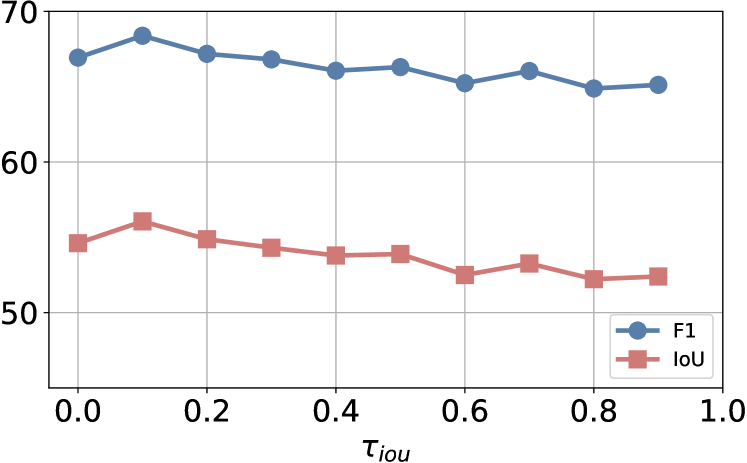
Figure 5: The impact of different thresholds of IoU on the HRSID-inshore dataset with 1-point.

IV-D3 Alternative IoU threshold

As mentioned earlier, NPC utilizes the IoU between masks to determine whether to use them as negative prompts. Hence, we evaluated the impact of different IoU thresholds in Eq.7 on the HRSID-inshore dataset, selecting values from 0 to 0.9 at intervals of 0.1. As shown in Fig. 5, the results peak at a threshold of 0.1. When the threshold is set to 0, the performance is slightly lower, likely due to the introduction of noisy prompts. As the IoU threshold increases beyond 0.1, both F1 and IoU metrics exhibit a downward trend. This decline is attributed to the reduced likelihood of negative prompt adjustments at higher thresholds, diminishing the influence of NPC.

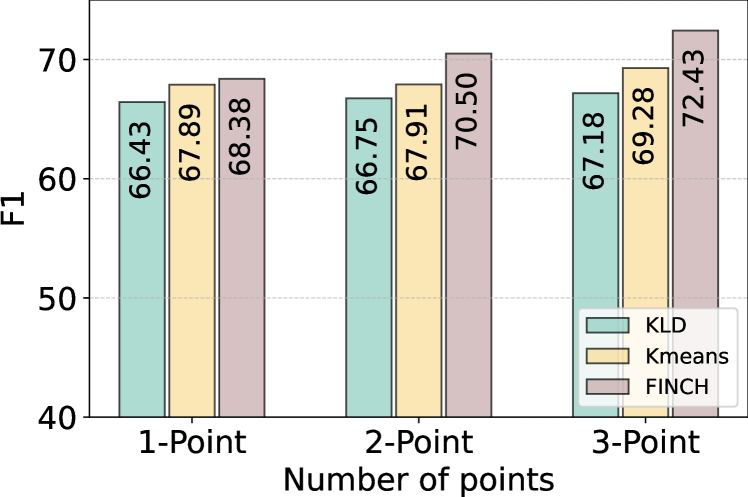
Figure 6: The comparison of the different feature clustering and alignment methods on the HRSID-inshore dataset.

IV-D4 Comparison with other feature alignment methods.

We compared different clustering and feature alignment methods, as shown in Fig. 6. KLD constrains the feature mean and variance of the source and target models on the target data using Kullback-Leibler divergence. Kmeans refers to the use of the Kmeans algorithm for feature clustering in PBR, while FINCH is the clustering method used in our work. The results show that FINCH outperforms other methods across various point settings.KLD performs poorly due to insufficient data, leading to inaccurate variance estimation. Kmeans performs slightly worse than FINCH because it requires manually set, fixed clustering centers that are not adaptive to the feature distribution. More importantly, it is more than three times slower than FINCH.

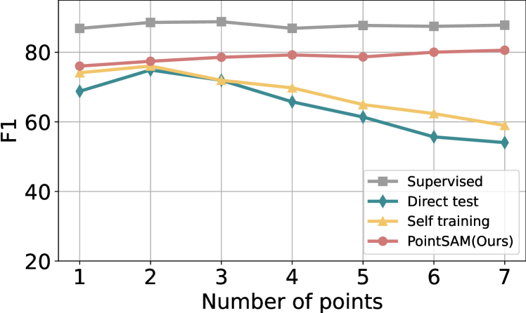
Figure 7: The impact of the number of points on different methods on the NWPU VHR-10 dataset.

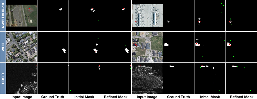
Figure 8: Visualization of the results of negative prompt calibration during training. The positive and negative prompts are represented by red points (•) and green points (•), respectively. The refined mask is generated from the initial mask after applying negative prompt calibration. This calibration effectively guides the negative prompts to more precise regions, enabling the generation of accurate masks.

IV-D5 How about more points?

We validated the results of different methods under an increased number of point prompts. As shown in Fig. 7, simply adding more points does not consistently lead to better performance. This is because increasing the number of points also raises the likelihood of including low-quality points. Such noise can negatively affect the segmentation results of other points. For the Supervised method, the results remained relatively unchanged due to the presence of full-mask constraints. Direct test achieved its best results with two points; however, as the number of points increased, the F1 score gradually decreased. Similarly, Self-training showed a decline in results due to the generation of noisy pseudo-labels. In contrast, our proposed PointSAM maintained stable results, approaching the performance of Supervised. This is because negative prompt calibration effectively corrected the prompts and reduced the impact of inaccurate masks caused by too many points.

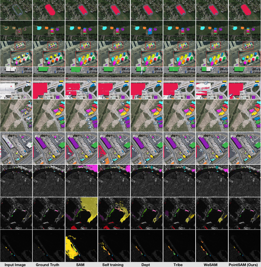
Figure 9: Comparison of visualization results for different methods. Rows 1-3 show the results on NWPU VHR-10 with 1 to 3 prompts; similarly, rows 4-6 display the results on WHU, and rows 7-9 show the results on HRSID-inshore. White arrows or zoom-ins in images are used to highlight.

IV-E Qualitative Evaluations

IV-E1 Visualization of the NPC Process

To visually demonstrate the effect of NPC during training, we present the results from the initial mask to the refined mask across three datasets. As shown in Fig. 8, the red points and green points represent positive prompts and negative prompts, respectively. In the first row for the NWPU VHR-10 dataset, the texture information of the tennis court is quite subtle, causing the initial mask to include an adjacent tennis court. After incorporating NPC, overlapping objects are treated as negative prompts, leading to the removal of excess masks. As the number of positive prompts increases, prompts located at the edges of objects are more likely to cause semantic ambiguity. This ambiguity can be accurately eliminated through NPC. For the buildings (second row) in the WHU dataset, they all have similar colors, which makes the mask indicated by the point prone to interference. Thanks to the large number of buildings in each image, NPC can easily locate nearby ambiguous masks, thus constraining the target mask. For the most challenging HRSID-inshore dataset, due to the SAR imaging mechanism, the color of each ship and the inshore scene appear identical (third row). Moreover, the targets are small and may be hollow. Therefore, if each negative prompt is constrained, a large amount of non-target regions will be designated as the mask. It can be seen that our method effectively suppresses redundant regions, regardless of the number of prompts.

IV-E2 Visualization of results from different methods

We then present the comparative results of different methods across various datasets. In the Fig. 9, rows 1-3 show the results on NWPU VHR-10 with 1 to 3 prompts; similarly, rows 4-6 display the results on WHU, and rows 7-9 show the results on HRSID-inshore. It can be observed that due to the bird’s-eye view in remote sensing images, there is a significant difference from natural images. Directly using the original SAM leads to an inability to distinguish each target clearly. For example, in the sixth row, the white building on the left and the parking lot on the right are treated as the same object. Even more notably, in the HRSID-inshore dataset, most of the inshore area is wrongly labeled as the target mask. Self-training transfers the source model to the target data, reducing more redundant areas and producing relatively more complete predicted masks compared to direct testing. However, it still fails to mitigate the interference between adjacent objects, such as the tennis court in the second row and the building in the fifth row. DePT, Tribe, and WeSAM are all improvements based on self-training, and they handle mask details better than self-training. However, in more challenging scenarios, they still fail to achieve optimal results. For example, in the third row, the storage tank and its shadow are not separated, and the ships in the inshore scene are not accurately segmented (rows 7-9). In contrast, our method excels at handling objects in dense scenes, achieving performance close to the ground truth.

IV-F PointSAM as a Detection Box Generator

In this section, we serve PointSAM as a point-to-box generator. PointSAM can generate corresponding masks based on points, and by calculating the minimum enclosing rectangle of the mask, we can obtain the corresponding horizontal bounding box (HBB). These HBBs can then be fed into a detector that converts horizontal boxes to rotated boxes, achieving point-supervised oriented object detection. To validate the effectiveness of this approach, we conducted experiments on the HRSID dataset, which includes both inshore and offshore scenarios. All experiments were conducted with an input size of 800×800, running for 12 epochs, and using ResNet-50 as the backbone. As shown in Table 6, we compared our method with representative algorithms based on OBB supervision, HBB supervision, and point supervision. It can be observed that the H2RBox-v2 and the method proposed by Yue et al. [71] based on HBB can achieve performance comparable to OBB supervision. The poor performance of H2RBox may be attributed to the large number of small objects in the HRSID dataset. Therefore, our approach also utilizes H2RBox as the detector for converting HBB to OBB. Compared to vanilla SAM, our method achieves a 15% improvement. This is because directly using SAM can result in unclear segmentation masks for objects in dense scenes, which in turn leads to inaccuracies in the minimum enclosing rectangles. Similarly, our method slightly outperforms Point2Rbox. Essentially, both Ours and Point2RBox leverage prior knowledge to learn the size information of the targets. There remains a gap of nearly 20% compared to the HBB-supervised methods. Future work could focus on integrating multiple types of priors to bridge this gap.

TABLE VI: Comparisons results of different detectors based on HRSID.

Methods	Backbone	recall(%)	AP50(%)
OBB-supervised
FCOS-O∗ [72]	ResNet-50	83.4	78.4
Faster RCNN-O∗ [73]	ResNet-50	83.1	78.0
RetinaNet-O [74]	ResNet-50	80.2	72.3
Oriented R-CNN [75]	ResNet-50	85.0	79.9
HBB-supervised
H2RBox [76]	ResNet-50	47.6	24.3
H2RBox-v2 [77]	ResNet-50	81.6	76.5
Yue et al. [71]	ResNet-50	85.0	81.5
Pointly-supervised
Point2RBox [38]	ResNet-50	64.2	57.1
SAM + H2RBox-v2	ResNet-50	56.6	44.7
PointSAM + H2RBox-v2 (Ours)	ResNet-50	68.9	59.5

V Conclusion

In this paper, we propose PointSAM, which adapts vanilla SAM to remote-sensing images using only point labels. Our method is based on a self-training framework. The proposed prototype-based regularization overcomes the issue of error accumulation in self-training by aligning prototypes predicted by the source and target models using the Hungarian matching algorithm. Negative prompt calibration effectively addresses the problem of densely distributed objects in RSIs by leveraging the spatial adjacency relationships of instances. Our method outperforms comparison algorithms on three widely used RSI datasets, NWPU VHR-10, HRSID, and WHU, and approaches the performance of supervised methods. Additionally, we also utilize the proposed PointSAM as a point-to-box generator to train a rotated box detector, achieving promising results. However, our method still has some issues to be improved. On the one hand, the self-training-based approach uses a dual-branch structure, which can result in slower training speeds. On the other hand, negative prompt calibration does not work well for objects with sparse distributions. Therefore, further consideration could be given to integrating information between images to effectively distinguish between foreground and background.

References

- Devlin et al. [2018] J. Devlin, M.-W. Chang, K. Lee, and K. Toutanova, “Bert: Pre-training of deep bidirectional transformers for language understanding,” arXiv preprint arXiv:1810.04805, 2018.
- Brown et al. [2020] T. Brown, B. Mann, N. Ryder, M. Subbiah, J. D. Kaplan, P. Dhariwal, A. Neelakantan, P. Shyam, G. Sastry, A. Askell et al., “Language models are few-shot learners,” Advances in neural information processing systems, vol. 33, pp. 1877–1901, 2020.
- Radford et al. [2021] A. Radford, J. W. Kim, C. Hallacy, A. Ramesh, G. Goh, S. Agarwal, G. Sastry, A. Askell, P. Mishkin, J. Clark et al., “Learning transferable visual models from natural language supervision,” in International conference on machine learning. PMLR, 2021, pp. 8748–8763.
- Jia et al. [2021] C. Jia, Y. Yang, Y. Xia, Y.-T. Chen, Z. Parekh, H. Pham, Q. Le, Y.-H. Sung, Z. Li, and T. Duerig, “Scaling up visual and vision-language representation learning with noisy text supervision,” in International conference on machine learning. PMLR, 2021, pp. 4904–4916.
- Kirillov et al. [2023] A. Kirillov, E. Mintun, N. Ravi, H. Mao, C. Rolland, L. Gustafson, T. Xiao, S. Whitehead, A. C. Berg, W.-Y. Lo et al., “Segment anything,” in Proceedings of the IEEE/CVF International Conference on Computer Vision, 2023, pp. 4015–4026.
- Ravi et al. [2024] N. Ravi, V. Gabeur, Y.-T. Hu, R. Hu, C. Ryali, T. Ma, H. Khedr, R. Rädle, C. Rolland, L. Gustafson, E. Mintun, J. Pan, K. V. Alwala, N. Carion, C.-Y. Wu, R. Girshick, P. Dollár, and C. Feichtenhofer, “Sam 2: Segment anything in images and videos,” arXiv preprint arXiv:2408.00714, 2024. [Online]. Available: https://arxiv.org/abs/2408.00714
- Ma et al. [2024] J. Ma, Y. He, F. Li, L. Han, C. You, and B. Wang, “Segment anything in medical images,” Nature Communications, vol. 15, no. 1, p. 654, 2024.
- Huang et al. [2024] Y. Huang, X. Yang, L. Liu, H. Zhou, A. Chang, X. Zhou, R. Chen, J. Yu, J. Chen, C. Chen et al., “Segment anything model for medical images?” Medical Image Analysis, vol. 92, p. 103061, 2024.
- Shan and Zhang [2023] X. Shan and C. Zhang, “Robustness of segment anything model (sam) for autonomous driving in adverse weather conditions,” arXiv preprint arXiv:2306.13290, 2023.
- Chen et al. [2024] K. Chen, C. Liu, H. Chen, H. Zhang, W. Li, Z. Zou, and Z. Shi, “Rsprompter: Learning to prompt for remote sensing instance segmentation based on visual foundation model,” IEEE Transactions on Geoscience and Remote Sensing, 2024.
- Wang et al. [2024] D. Wang, J. Zhang, B. Du, M. Xu, L. Liu, D. Tao, and L. Zhang, “Samrs: Scaling-up remote sensing segmentation dataset with segment anything model,” Advances in Neural Information Processing Systems, vol. 36, 2024.
- Xue et al. [2024] B. Xue, H. Cheng, Q. Yang, Y. Wang, and X. He, “Adapting segment anything model to aerial land cover classification with low-rank adaptation,” IEEE Geoscience and Remote Sensing Letters, vol. 21, pp. 1–5, 2024.
- Ding et al. [2024] L. Ding, K. Zhu, D. Peng, H. Tang, K. Yang, and L. Bruzzone, “Adapting segment anything model for change detection in vhr remote sensing images,” IEEE Transactions on Geoscience and Remote Sensing, 2024.
- Yan et al. [2023a] Z. Yan, J. Li, X. Li, R. Zhou, W. Zhang, Y. Feng, W. Diao, K. Fu, and X. Sun, “Ringmo-sam: A foundation model for segment anything in multimodal remote-sensing images,” IEEE Transactions on Geoscience and Remote Sensing, vol. 61, pp. 1–16, 2023.
- Pu et al. [2024] X. Pu, H. Jia, L. Zheng, F. Wang, and F. Xu, “Classwise-sam-adapter: Parameter efficient fine-tuning adapts segment anything to sar domain for semantic segmentation,” arXiv preprint arXiv:2401.02326, 2024.
- Zhang et al. [2023a] H. Zhang, Y. Su, X. Xu, and K. Jia, “Improving the generalization of segmentation foundation model under distribution shift via weakly supervised adaptation,” arXiv preprint arXiv:2312.03502, 2023.
- Xiao et al. [2024] A. Xiao, W. Xuan, H. Qi, Y. Xing, R. Ren, X. Zhang, and S. Lu, “Cat-sam: Conditional tuning network for few-shot adaptation of segmentation anything model,” arXiv preprint arXiv:2402.03631, 2024.
- Tang et al. [2024] L. Tang, Y. Yuan, C. Chen, K. Huang, X. Ding, and Y. Huang, “Bootstrap segmentation foundation model under distribution shift via object-centric learning,” arXiv preprint arXiv:2408.16310, 2024.
- Xu et al. [2021] M. Xu, Z. Zhang, H. Hu, J. Wang, L. Wang, F. Wei, X. Bai, and Z. Liu, “End-to-end semi-supervised object detection with soft teacher,” in Proceedings of the IEEE/CVF international conference on computer vision, 2021, pp. 3060–3069.
- VS et al. [2023] V. VS, P. Oza, and V. M. Patel, “Instance relation graph guided source-free domain adaptive object detection,” in Proceedings of the IEEE/CVF Conference on Computer Vision and Pattern Recognition, 2023, pp. 3520–3530.
- Liu et al. [2024a] N. Liu, X. Xu, Y. Su, C. Liu, P. Gong, and H.-C. Li, “Clip-guided source-free object detection in aerial images,” arXiv preprint arXiv:2401.05168, 2024.
- Liang et al. [2020] J. Liang, D. Hu, and J. Feng, “Do we really need to access the source data? source hypothesis transfer for unsupervised domain adaptation,” in Proc. Int. Conf. Mach. Learn. PMLR, 2020, pp. 6028–6039.
- Chen et al. [2023a] Y. Chen, X. Xu, Y. Su, and K. Jia, “Stfar: Improving object detection robustness at test-time by self-training with feature alignment regularization,” arXiv preprint arXiv:2303.17937, 2023.
- Mirza et al. [2023] M. J. Mirza, P. J. Soneira, W. Lin, M. Kozinski, H. Possegger, and H. Bischof, “Actmad: Activation matching to align distributions for test-time-training,” in Proceedings of the IEEE/CVF Conference on Computer Vision and Pattern Recognition, 2023, pp. 24 152–24 161.
- Yoo et al. [2024] J. Yoo, D. Lee, I. Chung, D. Kim, and N. Kwak, “What how and when should object detectors update in continually changing test domains?” in Proceedings of the IEEE/CVF Conference on Computer Vision and Pattern Recognition, 2024, pp. 23 354–23 363.
- Su et al. [2023] Y. Su, X. Xu, and K. Jia, “Towards real-world test-time adaptation: Tri-net self-training with balanced normalization,” 2023.
- Sarfraz et al. [2019] M. S. Sarfraz, V. Sharma, and R. Stiefelhagen, “Efficient parameter-free clustering using first neighbor relations,” in Proceedings of the IEEE Conference on Computer Vision and Pattern Recognition (CVPR), 2019, pp. 8934–8943.
- Zhang et al. [2023b] C. Zhang, D. Han, Y. Qiao, J. U. Kim, S.-H. Bae, S. Lee, and C. S. Hong, “Faster segment anything: Towards lightweight sam for mobile applications,” arXiv preprint arXiv:2306.14289, 2023.
- Xiong et al. [2024] Y. Xiong, B. Varadarajan, L. Wu, X. Xiang, F. Xiao, C. Zhu, X. Dai, D. Wang, F. Sun, F. Iandola et al., “Efficientsam: Leveraged masked image pretraining for efficient segment anything,” in Proceedings of the IEEE/CVF Conference on Computer Vision and Pattern Recognition, 2024, pp. 16 111–16 121.
- Ke et al. [2023] L. Ke, M. Ye, M. Danelljan, Y. Liu, Y.-W. Tai, C.-K. Tang, and F. Yu, “Segment anything in high quality,” in NeurIPS, 2023.
- Yuan et al. [2024a] H. Yuan, X. Li, C. Zhou, Y. Li, K. Chen, and C. C. Loy, “Open-vocabulary sam: Segment and recognize twenty-thousand classes interactively,” arXiv preprint arXiv:2401.02955, 2024.
- Ren et al. [2024] T. Ren, S. Liu, A. Zeng, J. Lin, K. Li, H. Cao, J. Chen, X. Huang, Y. Chen, F. Yan, Z. Zeng, H. Zhang, F. Li, J. Yang, H. Li, Q. Jiang, and L. Zhang, “Grounded sam: Assembling open-world models for diverse visual tasks,” 2024.
- Osco et al. [2023] L. P. Osco, Q. Wu, E. L. de Lemos, W. N. Gonçalves, A. P. M. Ramos, J. Li, and J. M. Junior, “The segment anything model (sam) for remote sensing applications: From zero to one shot,” International Journal of Applied Earth Observation and Geoinformation, vol. 124, p. 103540, 2023.
- Yan et al. [2023b] Z. Yan, J. Li, X. Li, R. Zhou, W. Zhang, Y. Feng, W. Diao, K. Fu, and X. Sun, “Ringmo-sam: A foundation model for segment anything in multimodal remote-sensing images,” IEEE Transactions on Geoscience and Remote Sensing, vol. 61, pp. 1–16, 2023.
- Moghimi et al. [2024] A. Moghimi, M. Welzel, T. Celik, and T. Schlurmann, “A comparative performance analysis of popular deep learning models and segment anything model (sam) for river water segmentation in close-range remote sensing imagery,” IEEE Access, 2024.
- Hu et al. [2021] E. J. Hu, Y. Shen, P. Wallis, Z. Allen-Zhu, Y. Li, S. Wang, L. Wang, and W. Chen, “Lora: Low-rank adaptation of large language models,” arXiv preprint arXiv:2106.09685, 2021.
- Chen et al. [2023b] K. Chen, C. Liu, W. Li, Z. Liu, H. Chen, H. Zhang, Z. Zou, and Z. Shi, “Time travelling pixels: Bitemporal features integration with foundation model for remote sensing image change detection,” arXiv preprint arXiv:2312.16202, 2023.
- Yu et al. [2024a] Y. Yu, X. Yang, Q. Li, F. Da, J. Dai, Y. Qiao, and J. Yan, “Point2rbox: Combine knowledge from synthetic visual patterns for end-to-end oriented object detection with single point supervision,” in IEEE/CVF Conference on Computer Vision and Pattern Recognition, 2024.
- Chen et al. [2022] P. Chen, X. Yu, X. Han, N. Hassan, K. Wang, J. Li, J. Zhao, H. Shi, Z. Han, and Q. Ye, “Point-to-box network for accurate object detection via single point supervision,” in European Conference on Computer Vision. Springer, 2022, pp. 51–67.
- Luo et al. [2024] J. Luo, X. Yang, Y. Yu, Q. Li, J. Yan, and Y. Li, “Pointobb: Learning oriented object detection via single point supervision,” in Proceedings of the IEEE/CVF Conference on Computer Vision and Pattern Recognition, 2024, pp. 16 730–16 740.
- Zhang et al. [2024] S. Zhang, J. Long, Y. Xu, and S. Mei, “Pmho: Point-supervised oriented object detection based on segmentation-driven proposal generation,” IEEE Transactions on Geoscience and Remote Sensing, pp. 1–1, 2024.
- Cao et al. [2023] G. Cao, X. Yu, W. Yu, X. Han, X. Yang, G. Li, J. Jiao, and Z. Han, “P2rbox: A single point is all you need for oriented object detection,” arXiv preprint arXiv:2311.13128, 2023.
- Fan et al. [2022] J. Fan, Z. Zhang, and T. Tan, “Pointly-supervised panoptic segmentation,” in European Conference on Computer Vision. Springer, 2022, pp. 319–336.
- Li et al. [2023] W. Li, Y. Yuan, S. Wang, J. Zhu, J. Li, J. Liu, and L. Zhang, “Point2mask: Point-supervised panoptic segmentation via optimal transport,” in Proceedings of the IEEE/CVF International Conference on Computer Vision, 2023, pp. 572–581.
- Bearman et al. [2016] A. Bearman, O. Russakovsky, V. Ferrari, and L. Fei-Fei, “What’s the point: Semantic segmentation with point supervision,” in European conference on computer vision. Springer, 2016, pp. 549–565.
- Cheng et al. [2022] B. Cheng, O. Parkhi, and A. Kirillov, “Pointly-supervised instance segmentation,” in Proceedings of the IEEE/CVF Conference on Computer Vision and Pattern Recognition, 2022, pp. 2617–2626.
- Yuan et al. [2024b] S. Yuan, H. Qin, R. Kou, X. Yan, Z. Li, C. Peng, and A.-K. Seghouane, “Beyond full label: Single-point prompt for infrared small target label generation,” arXiv preprint arXiv:2408.08191, 2024.
- Liu et al. [2021a] Y.-C. Liu, C.-Y. Ma, Z. He, C.-W. Kuo, K. Chen, P. Zhang, B. Wu, Z. Kira, and P. Vajda, “Unbiased teacher for semi-supervised object detection,” Proc. Int. Conf. Learn. Represent., 2021.
- Liu et al. [2024b] N. Liu, X. Xu, Y. Gao, Y. Zhao, and H.-C. Li, “Semi-supervised object detection with uncurated unlabeled data for remote sensing images,” International Journal of Applied Earth Observation and Geoinformation, vol. 129, p. 103814, 2024.
- Su et al. [2024] Y. Su, X. Xu, T. Li, and K. Jia, “Revisiting realistic test-time training: Sequential inference and adaptation by anchored clustering regularized self-training,” IEEE Transactions on Pattern Analysis and Machine Intelligence, 2024.
- Liu et al. [2024c] N. Liu, X. Xu, Y. Su, C. Liu, P. Gong, and H.-C. Li, “Clip-guided source-free object detection in aerial images,” arXiv preprint arXiv:2401.05168, 2024.
- Arazo et al. [2020] E. Arazo, D. Ortego, P. Albert, N. E. O’Connor, and K. McGuinness, “Pseudo-labeling and confirmation bias in deep semi-supervised learning,” in 2020 International joint conference on neural networks (IJCNN). IEEE, 2020, pp. 1–8.
- Zhao et al. [2022] Y. Zhao, T. Celik, N. Liu, and H.-C. Li, “A comparative analysis of gan-based methods for sar-to-optical image translation,” IEEE Geoscience and Remote Sensing Letters, vol. 19, pp. 1–5, 2022.
- Zhao et al. [2024] Y. Zhao, T. Celik, N. Liu, F. Gao, and H.-C. Li, “Sslchange: A self-supervised change detection framework based on domain adaptation,” arXiv preprint arXiv:2405.18224, 2024.
- Li et al. [2024] Y.-C. Li, S. Lei, N. Liu, H.-C. Li, and Q. Du, “Ida-siamnet: Interactive- and dynamic-aware siamese network for building change detection,” IEEE Transactions on Geoscience and Remote Sensing, vol. 62, pp. 1–13, 2024.
- Guo et al. [2023] P. Guo, T. Celik, N. Liu, and H.-C. Li, “Break through the border restriction of horizontal bounding box for arbitrary-oriented ship detection in sar images,” IEEE Geoscience and Remote Sensing Letters, vol. 20, pp. 1–5, 2023.
- Zhang et al. [2019] G. Zhang, S. Lu, and W. Zhang, “Cad-net: A context-aware detection network for objects in remote sensing imagery,” IEEE Transactions on Geoscience and Remote Sensing, vol. 57, no. 12, pp. 10 015–10 024, 2019.
- Gao et al. [2022a] G. Gao, Q. Liu, Z. Hu, L. Li, Q. Wen, and Y. Wang, “Psgcnet: A pyramidal scale and global context guided network for dense object counting in remote-sensing images,” IEEE Transactions on Geoscience and Remote Sensing, vol. 60, pp. 1–12, 2022.
- Liu et al. [2021b] N. Liu, T. Celik, T. Zhao, C. Zhang, and H.-C. Li, “Afdet: Toward more accurate and faster object detection in remote sensing images,” IEEE Journal of Selected Topics in Applied Earth Observations and Remote Sensing, vol. 14, pp. 12 557–12 568, 2021.
- Yang and Yan [2020] X. Yang and J. Yan, “Arbitrary-oriented object detection with circular smooth label,” in Computer Vision–ECCV 2020: 16th European Conference, Glasgow, UK, August 23–28, 2020, Proceedings, Part VIII 16. Springer, 2020, pp. 677–694.
- Fu et al. [2023] B. Fu, W. Li, Y. Sun, G. Chen, L. Zhang, and W. Wei, “Correlated nms: Establishing correlations between dense predictions of remote sensing images,” in IGARSS 2023 - 2023 IEEE International Geoscience and Remote Sensing Symposium, 2023, pp. 6153–6156.
- Guo et al. [2021] W. Guo, W. Li, W. Gong, and C. Chen, “Region-attentioned network with location scoring dynamic-threshold nms for object detection in remote sensing images,” in Proceedings of the 2020 4th International Conference on Vision, Image and Signal Processing, ser. ICVISP 2020. New York, NY, USA: Association for Computing Machinery, 2021. [Online]. Available: https://doi.org/10.1145/3448823.3448824
- Dosovitskiy [2020] A. Dosovitskiy, “An image is worth 16x16 words: Transformers for image recognition at scale,” arXiv preprint arXiv:2010.11929, 2020.
- Carion et al. [2020] N. Carion, F. Massa, G. Synnaeve, N. Usunier, A. Kirillov, and S. Zagoruyko, “End-to-end object detection with transformers,” in European conference on computer vision. Springer, 2020, pp. 213–229.
- Stewart et al. [2016] R. Stewart, M. Andriluka, and A. Y. Ng, “End-to-end people detection in crowded scenes,” in Proceedings of the IEEE Conference on Computer Vision and Pattern Recognition (CVPR), June 2016.
- Wei et al. [2020] S. Wei, X. Zeng, Q. Qu, M. Wang, H. Su, and J. Shi, “Hrsid: A high-resolution sar images dataset for ship detection and instance segmentation,” Ieee Access, vol. 8, pp. 120 234–120 254, 2020.
- Cheng et al. [2016] G. Cheng, P. Zhou, and J. Han, “Learning rotation-invariant convolutional neural networks for object detection in vhr optical remote sensing images,” IEEE transactions on geoscience and remote sensing, vol. 54, no. 12, pp. 7405–7415, 2016.
- Ji et al. [2018] S. Ji, S. Wei, and M. Lu, “Fully convolutional networks for multisource building extraction from an open aerial and satellite imagery data set,” IEEE Transactions on geoscience and remote sensing, vol. 57, no. 1, pp. 574–586, 2018.
- Wang et al. [2021] D. Wang, E. Shelhamer, S. Liu, B. Olshausen, and T. Darrell, “Tent: Fully test-time adaptation by entropy minimization,” Proc. Int. Conf. Learn. Represent., 2021.
- Gao et al. [2022b] Y. Gao, X. Shi, Y. Zhu, H. Wang, Z. Tang, X. Zhou, M. Li, and D. N. Metaxas, “Visual prompt tuning for test-time domain adaptation,” arXiv preprint arXiv:2210.04831, 2022.
- Yue et al. [2024] T. Yue, Y. Zhang, J. Wang, Y. Xu, and P. Liu, “A weak supervision learning paradigm for oriented ship detection in sar image,” IEEE Transactions on Geoscience and Remote Sensing, vol. 62, pp. 1–12, 2024.
- Tian et al. [2019] Z. Tian, C. Shen, H. Chen, and T. He, “Fcos: Fully convolutional one-stage object detection,” in 2019 IEEE/CVF International Conference on Computer Vision (ICCV), 2019, pp. 9626–9635.
- Ren et al. [2015] S. Ren, K. He, R. Girshick, and J. Sun, “Faster R-CNN: Towards real-time object detection with region proposal networks,” in Advances in Neural Information Processing Systems (NIPS), 2015.
- Yang et al. [2021] X. Yang, X. Yang, J. Yang, Q. Ming, W. Wang, Q. Tian, and J. Yan, “Learning high-precision bounding box for rotated object detection via kullback-leibler divergence,” Advances in Neural Information Processing Systems, vol. 34, pp. 18 381–18 394, 2021.
- Xie et al. [2024] X. Xie, G. Cheng, J. Wang, K. Li, X. Yao, and J. Han, “Oriented r-cnn and beyond,” International Journal of Computer Vision, pp. 1–23, 2024.
- Yang et al. [2022] X. Yang, G. Zhang, W. Li, X. Wang, Y. Zhou, and J. Yan, “H2rbox: Horizontal box annotation is all you need for oriented object detection,” arXiv preprint arXiv:2210.06742, 2022.
- Yu et al. [2024b] Y. Yu, X. Yang, Q. Li, Y. Zhou, F. Da, and J. Yan, “H2rbox-v2: Incorporating symmetry for boosting horizontal box supervised oriented object detection,” Advances in Neural Information Processing Systems, vol. 36, 2024.