A high-order implicit time integration method for linear and nonlinear dynamics with efficient computation of accelerations

Abstract

An algorithm for a family of self-starting high-order implicit time integration schemes with controllable numerical dissipation is proposed for both linear and nonlinear transient problems. This work builds on the previous works of the authors on elastodynamics by presenting a new algorithm that eliminates the need for factorization of the mass matrix providing benefit for the solution of nonlinear problems. The improved algorithm directly obtains the acceleration at the same order of accuracy of the displacement and velocity using vector operations (without additional equation solutions). The nonlinearity is handled by numerical integration within a time step to achieve the desired order of accuracy. The new algorithm fully retains the desirable features of the previous works: 1. The order of accuracy is not affected by the presence of external forces and physical damping; 2. The amount of numerical dissipation in the algorithm is controlled by a user-specified parameter $\rho_{\infty}$, leading to schemes ranging from perfectly nondissipative $A$-stable to $L$-stable; 3. The effective stiffness matrix is a linear combination of the mass, damping, and stiffness matrices as in the trapezoidal rule, leading to high efficiency for large-scale problems. The proposed algorithm, with its elegance and computational advantages, is shown to replicate the numerical results demonstrated on linear problems in previous works. Additional numerical examples of linear and nonlinear vibration and wave propagation are presented herein. Notably, the proposed algorithms show the same convergence rates for nonlinear problems as linear problems, and very high accuracy. It was found that second-order time integration methods commonly used in commercial software produce significantly polluted acceleration responses for a common class of wave propagation problems. The high-order time integration schemes presented here perform noticably better at suppressing spurious high-frequency oscillations and producing reliable and useable acceleration responses. The source code written in MATLAB is available for download at: $\rm{https://github.com/ChongminSong/HighOrderTimeIngt\_PartialFraction.git}$

1 Introduction

Direct time integration schemes are employed in the numerical simulation of time-dependent problems in many disciplines of engineering and science. The requirements for an effective time integration scheme may vary according to the applications. For some classes of applications, such as celestial motions [1], the equation of motion is directly formulated as an initial value problem of ordinary differential equations. A sufficiently accurate approximation of the exact solution of the ordinary differential equations under given initial conditions is required. Several well-known classes of numerical methods, such as single-step Euler methods, linear multi-step methods and Runge–Kutta methods using intermediate sub-steps, have been widely studied and implemented in computer software libraries, see e.g., [2, 3].

There are many engineering applications where the governing equations are formulated as partial differential equations in time and space. One type of such applications addressed in this paper is the problem of wave propagation in the continuum. Typically, the problem domain is first discretized spatially by the finite element method [4, 5] or other numerical methods. The resulting semi-discrete equation of motion is expressed as a system of ordinary differential equations in time. The spatial discretization techniques are accurate for low-frequency modes, but introduce large dispersion errors for high-frequency modes [6, 7, 8, 9]. When high-frequency modes are excited, the solution to the ordinary differential equations will be polluted by spurious (i.e., non-physical) oscillations. Therefore, time integration schemes aiming to obtain the exact solution of the ordinary differential equations, such as the Runge–Kutta methods, are not used in finite element software packages for structural analysis. A large number of direct time integration schemes aiming to achieve high-frequency dissipation while minimizing low-frequency dissipation have been developed in the area of structural dynamics. Only implicit schemes are addressed in this paper.

Many implicit time integration methods that have the capacity of introducing numerical dissipation of high-frequency modes have been developed, e.g., [10, 11, 12, 13, 14, 15, 16, 17, 18, 19, 20, 21, 22, 23, 24, 25] to name a few. The integration methods that are most commonly found in commercial finite element packages include the Houbolt method [10], the Wilson-$\theta$ method [12], the Newmark method [11], the HHT-$\alpha$ method [13], and the generalized-$\alpha$ method [15]. All of these methods are second-order accurate and share a common characteristic: the effective stiffness matrix of the implicit equation has the same sparsity and size as those of the static stiffness matrix, ensuring high computational efficiency in time-stepping. In practical applications, two parameters are typically selected: one is the time step size, and the other is a parameter controlling the amount of numerical dissipation. For the same numerical dissipation parameter, reducing the time step size will also reduce the amount of numerical dissipation. Therefore, a smaller time step size does not necessarily lead to a smaller solution error in the sense of engineering application [23]. The optimal choice of the time step size for a given time integration scheme is conventionally recommended as a Courant-Friedrichs-Lewy (CFL) number.

Various high-order time integration methods that have an order of accuracy higher than two have been proposed  [14, 26, 17, 19, 27, 28, 29, 21, 30, 31, 22, 8, 32]. In comparison with standard second-order time integration schemes, the potential benefits are twofold: 1) A much larger time step size can be used to obtain a solution of similar accuracy (although it is more expensive to advance one time step, the overall performance can be more efficient), and 2) The numerical dissipation can be more effectively controlled, i.e., stronger high-frequency dissipation and less low-frequency dissipation. Numerical methods such as collocation, differential quadrature, weighted residuals, and matrix exponentials are applied to derive the time-stepping formulations. Reviews on the recent progress have been reported by the authors in [33, 34]. Most of the high-order time integration methods either increase the size or destroy the sparsity of the implicit equation, and, as a result, the computational cost increases rapidly with the problem size. These methods are then not capable of handling problems of as large a size as the conventional second-order methods can.

Composite time integration approaches, which are constructed by splitting a single time step into two or more sub-steps, have been adopted in many recent works [16, 35, 36, 37, 38, 39, 29, 20, 40, 41, 42, 43, 23, 44, 32, 45, 46]. By judiciously choosing different time integration methods or different values of the parameters for the individual sub-steps, improved accuracy and numerical properties are achieved. A comprehensive review and an attempt to unify the different formulations have been reported by Kim and Reddy in [47]. The Bathe method has been extended to third-order and fourth-order accuracy in [44, 32]. A high-order composite time integration method is proposed in [45], where the accuracy order equals the number of sub-steps.

Self-starting with the initial displacement and velocity is a desirable property of a time integration method  [48]. Self-starting implicit methods have been reported in [43, 49, 45, 25], to name a few. As the initial acceleration is not required, the factorization of the mass matrix becomes unnecessary. This reduces the computational time and memory costs when a consistent mass matrix is used [43]. In situations where acceleration responses are needed, for example, in earthquake engineering and in structural health monitoring employing accelerometers, the acceleration can be obtained from the interpolation built in the schemes when the accuracy order is not higher than three [45, 25]. To maintain the same order of accuracy with the displacement and velocity in a higher-order scheme, the acceleration needs to be solved from the equation of motion, thus requiring factorization of the mass matrix and compromising the computational advantages of high-order self-starting methods.

A family of computationally effective high-order time integration schemes has been developed in [9, 34] by designing rational approximations of the matrix exponential in the analytical solution of the equation of motion. A salient feature of these schemes is that the effective stiffness matrix is a linear combination of the mass, damping, and stiffness matrices, similar to the conventional second-order methods such as the trapezoidal rule and Newmark method. These schemes conform to the concept of the composite time integration method, where the solution at the intermediate time point is only used to calculate the solution at the full step [35, 44, 29]. Two types of rational approximations are adopted. In [9], the numerical dissipation is controlled by mixing the Padé expansions of orders $(M,M)$ and $(M-1,M)$. When the rational function is a Padé expansion of order $(M,M)$, i.e., the diagonal Padé expansion, the scheme is strictly non-dissipative, $2M$-th order accurate and A-stable. Otherwise, the scheme is dissipative and $(2M-1)$-th order accurate. At the other extreme, the Padé expansion of order $(M-1,M)$ leads to an $L$-stable scheme. Each solution of an implicit equation increases the order of accuracy by one when the effective stiffness matrix is real and by two when the effective stiffness matrix is complex. In  [34], the denominator of the rational approximation is selected to have one real root, i.e., a single multiple root. Unconditionally stable schemes up to the sixth-order accuracy are identified. Each solution of an implicit equation increases the order of accuracy by one. In this approach, the effective stiffness matrices of all the implicit equations are the same, reducing the computational cost of matrix factorization when a direct solver is used. Although the algorithm in [9, 34] is self-starting without using the acceleration for time-stepping, the algorithm requires the factorization of the mass matrix to compute $\mathbf{M}^{-1}\mathbf{f}$, where $\mathbf{M}$ is the mass matrix and $\mathbf{f}$ is the external force vector, and therefore the full benefits of a self-starting algorithm are not realized. In a nonlinear analysis, this operation incurs additional computational cost since the force vector $\mathbf{f}$ within a time step is unknown beforehand. .

This paper introduces a new time-stepping algorithm for the family of high-order schemes in [9, 34], and demonstrates their performance on a range of linear and nonlinear transient problems. Using partial fractions of the rational approximations, this algorithm eliminates the need to compute $\mathbf{M}^{-1}\mathbf{f}$, and instead it is sufficient to sample the force vector $\mathbf{f}$ at specified time instances, leading to a family of efficient high-order schemes for nonlinear dynamics. Furthermore, a new formulation to compute the acceleration is developed, which involves only vector operations and no additional equation solutions. The order of accuracy remains the same as that of the displacement and velocity, i.e., equal to the order of the time integration scheme. It is worthwhile to reemphasize that acceleration is not needed for the time-stepping and the algorithm itself is self-starting. The factorization of the mass matrix becomes unnecessary even if high-order accuracy of acceleration is required. The full benefits of a self-starting algorithm are realized for both nonlinear and linear cases. In numerical examples, the proposed algorithms show the same convergence rates for nonlinear problems as linear problems, and very high accuracy.

The remainder of the paper is organized as follows: Section 2 presents the time-stepping solution scheme using matrix exponentials, including analytic treatment of the non-homogeneous term using a series expansion of the excitation force vector and a recursive scheme to evaluate the integrals. Section 3 presents the rational approximation of the matrix exponential using Padé expansions. Section 4 presents the algorithmic novelty of the work, deriving time-stepping algorithms that eliminate the need to compute $\mathbf{M}^{-1}\mathbf{f}$ terms through expansions using partial fractions for cases where the divisor polynomial possesses either 1) distinct roots, or 2) a single multiple root. Solutions to the time-stepping equation for both cases have an identical representation which is presented in Section 5. In Section 6, the algorithm to obtain acceleration to the same order of accuracy as displacement without additional equation solution and using only vector operations is developed. Discussion on treatment of the non-homogeneous term is offered in Section 7, with sample algorithms for the time-stepping procedures presented in Section 8. Section 9 provides a range of numerical examples which demonstrate the efficacy of the proposed approach on accurately modelling both linear and nonlinear dynamic problems, followed by conclusions drawn.

Additional examples of using the algorithms herein are presented in the Appendix, alongside sample MATLAB code for many of the important functions used.

2 Time-stepping scheme using rational approximation of matrix exponential

For a structural dynamics problem, the governing equations of motion are expressed as a system of second-order ODEs as follows:

$$\mathbf{M\ddot{u}}(t)+\mathbf{f}_{I}(\mathbf{u}(t),\mathbf{\dot{u}}(t))=\mathbf{f}_{E}(t)\,,\thinspace\thinspace\thinspace\mathbf{u}_{0}=\mathbf{u}(0),\thinspace\dot{\mathbf{u}}_{0}=\dot{\mathbf{u}}(0)\thinspace,$$ (1)

where $\mathbf{M}$ denotes the mass matrix, $\mathbf{f}_{I}$ gives the internal force vector, and $\mathbf{f}_{E}$ represents the external excitation force. The vectors $\mathbf{u}$, $\dot{\mathbf{u}}$ and $\mathbf{\ddot{u}}$ denote the displacement, velocity, and acceleration, respectively, each a function of time $t$, and $\mathbf{u}_{0},\dot{\mathbf{u}}_{0}$ provide the initial conditions. Using a series expansion about time $t=t_{n-1}$, the linear part of the internal force vector can be separated from the nonlinear remainder such that

$$\mathbf{M}\mathbf{\ddot{u}}(t)+\mathbf{C}_{n-1}\mathbf{\dot{u}}(t)+\mathbf{K}_{n-1}\mathbf{u}(t)=\mathbf{f}(\mathbf{u}(t),\dot{\mathbf{u}}(t))\,,$$ (2)

with

$$\mathbf{C}(t)=\frac{\partial\mathbf{f}_{I}}{\partial\dot{\mathbf{u}}}\,,\thinspace\thinspace\thinspace\mathbf{K}(t)=\frac{\partial\mathbf{f}_{I}}{\partial\mathbf{u}}\thinspace,$$ (3)

denoting tangent damping and stiffness matrices at time $t$, respectively, and the right-hand side of Eq. (2) being described by the nonlinear force vector

$$\mathbf{f}(\mathbf{u}(t),\dot{\mathbf{u}}(t))=\mathbf{f}_{E}(t)-\mathbf{f}_{I}(\mathbf{u}(t),\mathbf{\dot{u}}(t))+\mathbf{C}_{n-1}\mathbf{\dot{u}}(t)+\mathbf{K}_{n-1}\mathbf{u}(t)\ .$$ (4)

The above equations of motion (Eq. (2)) are now considered in the time step $n$, denoting the time interval $t_{n-1}\leq t\leq t_{n}$ (for $n=1,2,3,\ldots$). The time step size is thus defined such that $\Delta t=t_{n}-t_{n-1}$. By introducing a dimensionless time variable $s,$ any point in time within a given time step $n$ can be determined by

$$t(s)=t_{n-1}+s\Delta t,\quad\;0\leq s\leq 1\,,$$ (5)

with $t(0)=t_{n-1}$ and $t(1)=t_{n}$ returning the beginning and end of the time step, respectively. In this work, the derivative of a quantity with respect to the dimensionless time $s$ is denoted through the use of a circle ($\circ$) above the symbol. The incremental velocity and acceleration vectors within a given time step $t_{n-1}\leq t\leq t_{n}$ are therefore represented as

$$\mathbf{\dot{u}}=\frac{1}{\Delta t}\frac{\mathrm{d\mathbf{u}}}{\mathrm{d}s}=\frac{1}{\Delta t}\overset{\circ}{\mathbf{u}}\,,$$ (6)

$$\mathbf{\ddot{u}}=\frac{1}{\Delta t^{2}}\frac{\mathrm{d^{2}\mathbf{u}}}{\mathrm{d}s^{2}}=\frac{1}{\Delta t^{2}}\overset{\circ\circ}{\mathbf{u}}\,.$$ (7)

Therefore, the equations of motion (Eq. (2)) can now be expressed with respect to the dimensionless time as:

$$\mathbf{M}\overset{\circ\circ}{\mathbf{u}}(t)+\Delta t\,\mathbf{C}_{n-1}\overset{\circ}{\mathbf{u}}(t)+\Delta t^{2}\,\mathbf{K}_{n-1}\mathbf{u}(t)=\Delta t^{2}\,\mathbf{f}(\mathbf{z}(t))\,.$$ (8)

Equation (8) can be transformed into a system of first-order ODEs by introducing a state-space vector $\mathbf{z}$ defined as

$$\mathbf{z}(t)=\begin{Bmatrix}\overset{\circ}{\mathbf{u}}(t)\\ \mathbf{u}(t)\end{Bmatrix}\,,$$ (9)

and subsequently taking the derivative of $\mathbf{z}$ with respect to $s$:

$$\overset{\circ}{\mathbf{z}}(t)\equiv\frac{\mathrm{d\mathbf{z}}}{\mathrm{d}s}=\mathbf{A}\mathbf{z}(t)+\overline{\mathbf{f}}(\mathbf{z}(t))\,.$$ (10)

Here, $\mathbf{A}$ is the tangent coefficient matrix at time $t_{n-1}$ defined as

$$\mathbf{\mathbf{A}}=\begin{bmatrix}-\Delta t\mathbf{M}^{-1}\mathbf{C}_{n-1}&-\Delta t^{2}\mathbf{M}^{-1}\mathbf{K}_{n-1}\\ \mathbf{I}&\mathbf{0}\end{bmatrix}\,,$$ (11)

and $\overline{\mathbf{f}}$ is the nonlinear force vector (at time $t$) given by:

$$\overline{\mathbf{f}}(\mathbf{z}(t))=\begin{Bmatrix}\Delta t^{2}\ \mathbf{M}^{-1}\mathbf{f}(\mathbf{z}(t))\\ \mathbf{0}\end{Bmatrix}.$$ (12)

The analytical solution to the system of first-order ODEs given by Eq. (10) is expressed using the matrix exponential function as

$$\mathbf{z}(t_{n-1}+s\Delta t)=e^{\mathbf{A}s}\mathbf{z}_{n-1}+e^{\mathbf{A}s}\intop_{0}^{s}e^{-\mathbf{A}\tau}\overline{\mathbf{f}}(\mathbf{z}(t_{n-1}+\tau\thinspace\Delta t))\mathrm{d}\tau\,.$$ (13)

2.1 Analytical approximation of non-homogeneous term

Following [33], the integration in Eq. (13) is performed analytically by approximating the vector $\mathbf{f}$ with Taylor expansion of order $p_{\mathrm{f}}$ at the mid-point of the time step $n$

$$\mathbf{f}(s)=\sum\limits_{k=0}^{p_{\mathrm{f}}}\tilde{\mathbf{f}}^{(k)}(s-0.5)^{k}=\tilde{\mathbf{f}}^{(0)}+\tilde{\mathbf{f}}^{(1)}(s-0.5)+\tilde{\mathbf{f}}^{(2)}(s-0.5)^{2}+\ldots+\tilde{\mathbf{f}}^{(p_{\mathrm{f}})}(s-0.5)^{p_{\mathrm{f}}}\,,$$ (14)

where $\tilde{\mathbf{f}}^{(k)}$ ($k=0,\,1,\,2,\,\ldots,\,p_{\mathrm{f}}$) denotes the $k$-th order derivatives of the vector $\mathbf{f}$. This series expansion is compactly written as the matrix-vector product

$$\mathbf{f}(s)=\tilde{\mathbf{F}}\cdot\mathbf{s}(s)\,,$$ (15)

with the columns of matrix $\tilde{\mathbf{F}}$ storing force-derivatives vectors and the vector $\mathbf{s}$ storing powers of $(s-0.5)$ according to

$$\tilde{\mathbf{F}}=\left[\begin{array}[]{ccccc}\tilde{\mathbf{f}}^{(0)}&\tilde{\mathbf{f}}^{(1)}&\tilde{\mathbf{f}}^{(2)}&\ldots&\tilde{\mathbf{f}}^{(p_{\mathrm{f}})}\end{array}\right]\,,$$ (16)

and

$$\mathbf{s}(s)=\left[\begin{array}[]{ccccc}1&(s-0.5)&(s-0.5)^{2}&\ldots&(s-0.5)^{p_{\mathrm{f}}}\end{array}\right]^{\mathrm{T}}\,.$$ (17)

The evaluation of matrix $\tilde{\mathbf{F}}$ from the force $\mathbf{f}$ at specified time instances is discussed in Section 7.

Substituting Eq. (14) into Eq. (13), the solution at the end of time step $t_{n}$ (i.e., $s=1$) is obtained as

$$\mathbf{z}_{n}=e^{\mathbf{A}}\mathbf{z}_{n-1}+\sum\limits_{k=0}^{p_{\mathrm{f}}}\mathbf{B}_{k}\left\{\begin{array}[]{c}\Delta t^{2}\thinspace\mathbf{M^{-1}}\tilde{\mathbf{f}}^{(k)}\\ \mathbf{0}\end{array}\right\}\,,$$ (18)

where the matrices $\mathbf{B}_{k}$ are obtained through integration by parts and can be determined recursively:

$$\begin{split}\mathbf{B}_{k}&=\mathbf{A}^{-1}\left(k\mathbf{B}_{k-1}+\left(-\tfrac{1}{2}\right)^{k}\left(e^{\mathbf{A}}-(-1)^{k}\mathbf{I}\right)\right)\,,\quad\;\forall k=0,1,2,\ldots,p_{\mathrm{f}}\,,\end{split}$$ (19)

with the starting value at $k=0$ given by

$$\mathbf{B}_{0}=\mathbf{A}^{-1}\left(e^{\mathbf{A}}-\mathbf{I}\right)\,.$$ (20)

3 Rational approximation of matrix exponential

To derive an efficient time-stepping scheme, Padé expansions are often employed (see [33, 9]) to approximate the matrix exponential $e^{\mathbf{A}}$. Here, the roots of the denominator polynomial are all distinct and can be either real or complex. In [34], a rational approximation is constructed in such a way that the denominator possesses only a single real root. The proposed time-stepping scheme based on partial fractions is applicable to both cases of real or complex roots. For generality, the following rational approximation $\mathbf{R}=R(\mathbf{A})$ of the matrix exponential $e^{\mathbf{A}}$ is considered

$$e^{\mathbf{A}}\approx\mathbf{R}=\mathbf{\dfrac{\mathbf{P}}{Q}}=\dfrac{p_{0}\mathbf{I}+p_{1}\mathbf{A}+\ldots+p_{M}\mathbf{A}^{M}}{q_{0}\mathbf{I}+q_{1}\mathbf{A}+\cdots+q_{M}\mathbf{A}^{M}}\,,$$ (21)

where $\mathbf{P}=P(\mathbf{A})$ and $\mathbf{Q}=Q(\mathbf{A})$ are polynomials of matrix $\mathbf{A}$ of order $M$. Note that the matrix product $\mathbf{Q}^{-1}\mathbf{P}$ is commutative (i.e., $\mathbf{P}\mathbf{Q}^{-1}=\mathbf{Q}^{-1}\mathbf{\mathbf{P}}$), and the scalar coefficients $p_{i}$ and $q_{i}$ are real numbers. To ensure that $e^{\mathbf{0}}=\mathbf{I}$ holds, it is necessary for $p_{0}=q_{0}$. For a stable time-stepping scheme, it is necessary to have $q_{M}\neq 0$ and $|p_{M}/q_{M}|=\rho_{\infty}\leq 1$, where $\rho_{\infty}$ denotes the spectral radius at the high-frequency limit. When $p_{M}=0$, it follows that $\rho_{\infty}=0$ and the scheme is ‘$L$-stable’.

Replacing the matrix exponential $e^{\mathbf{A}}$ in Eqs. (18), (19) and (20) with the rational approximation in Eq. (21), the time-stepping equation becomes

$$\mathbf{z}_{n}=\frac{\mathbf{P}}{\mathbf{Q}}\mathbf{z}_{n-1}+\frac{1}{\mathbf{Q}}\sum\limits_{k=0}^{p_{\mathrm{f}}}\mathbf{C}_{k}\left\{\begin{array}[]{c}\Delta t^{2}\mathbf{M^{-1}}\tilde{\mathbf{f}}^{(k)}\\ \mathbf{0}\end{array}\right\}\,,$$ (22)

where the matrices $\mathbf{C}_{k}$ (not to be confused with the tangent damping matrix in Eq. (3)) are obtained from Eqs. (19) and (21) through the following recursive relation

$$\mathbf{C}_{k}=\mathbf{Q}\mathbf{B}_{k}=\mathbf{A}^{-1}\left(k\mathbf{C}_{k-1}+\left(-0.5\right)^{k}(\mathbf{P}-(-1)^{k}\mathbf{Q})\right);\qquad(k=1,2,\ldots,p_{\mathrm{f}})\,,$$ (23)

which are evaluated starting from

$$\mathbf{C}_{0}=\mathbf{Q}\mathbf{B}_{0}=\mathbf{A}^{-1}\left(\mathbf{P}-\mathbf{Q}\right)\,,$$ (24)

using $\mathbf{B}_{0}$ in Eq. (20). Since both $\mathbf{P}$ and $\mathbf{Q}$ are matrix polynomials of order $M$ , the matrices $\mathbf{C}_{k}$ ($k=0,1,\ldots,p_{\mathrm{f}}$) are matrix polynomials with degrees at most $M-1$. They can hence be expanded by the power series

$$\mathbf{C}_{k}=C_{k}(\mathbf{A})=c_{k0}\mathbf{I}+c_{k1}\mathbf{A}+\ldots+c_{k(M-1)}\mathbf{A}^{M-1}=\sum_{i=0}^{M-1}c_{ki}\mathbf{A}^{i};\qquad(k=0,1,\ldots p_{\mathrm{f}})\,,$$ (25)

where $c_{ki}$ are scalar coefficients; stored for later use in a coefficient matrix $\mathbf{c}$:

$$\mathbf{c}=[c_{ki}];\qquad(k=0,1,\ldots p_{\mathrm{f}};\quad i=0,1,\ldots,M-1)\,.$$ (26)

4 Partial fraction expansion of rational approximations

The time-stepping solution in Eq. (22) has been used to produce self-starting high-order time integration schemes with controllable numerical dissipation in [33, 9, 34], and performance tested against a range of numerical examples. In those works, the algorithms used to execute the time-stepping schemes required calculation of the $\mathbf{M}^{-1}\tilde{\mathbf{f}}^{(k)}$ terms in Eq. (22), plus additional equations solutions to determine the acceleration. Therefore, whilst the algorithms were self-starting, the full benefit of a self-starting algorithm (that is, avoiding factorization of the mass matrix, or extraneous equation solutions) were not realized. The computational benefit of avoiding calculation of $\mathbf{M}^{-1}\mathbf{f}$ terms in time-stepping algorithms is most prominent in nonlinear problems where $\mathbf{f}$ is unknown within the current time step, and iterative solution procedures require additional calculations to be made.

In this section, a new approach to deriving an efficient time-stepping scheme is presented by applying partial fraction expansion of the rational functions $\mathbf{P}/\mathbf{Q}$ and $\mathbf{C}_{k}/\mathbf{Q}$ ($k=1,\,2,\,\ldots,\,p_{\mathrm{f}}$) that are present in Eq. (22). The general case of the divisor polynomial $\mathbf{Q}$ having distinct roots is discussed in Section 4.1, followed by the specialized case of $\mathbf{Q}$ possessing a single multiple real root presented in Section 4.2. The algorithmic implementation of both is then discussed. The algorithms avoid any calculation of terms of the form $\mathbf{M}^{-1}\cdot\mathbf{f}$; and also allow acceleration to be calculated at the same order of accuracy as displacment and velocity using only vector operations. Sample MATLAB code with illustrative examples are provided in A.

4.1 Case 1: Distinct roots

4.1.1 Evaluation of matrix exponential

Consider that the polynomial $Q(\mathbf{A})$ possesses distinct roots, so the rational approximation Eq. (21) is evaluated according to the Padé expansion as outlined in [9]. Both the numerator $\mathbf{P}$ and denominator $\mathbf{Q}$ in Eq. (21) are selected as polynomials of order $M$. To begin the derivation, the rational expansion in Eq. (21) is first decomposed as

$$\mathbf{\dfrac{\mathbf{P}}{Q}}=\dfrac{p_{M}}{q_{M}}\mathbf{I}+\dfrac{p_{l0}\mathbf{I}+p_{l1}\mathbf{A}+\ldots+p_{l(M-1)}\mathbf{A}^{M-1}}{q_{0}\mathbf{I}+q_{1}\mathbf{A}+\cdots+q_{M}\mathbf{A}^{M}}=\dfrac{p_{M}}{q_{M}}\mathbf{I}+\dfrac{\mathbf{P}_{\mathrm{L}}}{\mathbf{Q}}\,,$$ (27)

where ${p_{M}}/{q_{M}}$ is the ratio of coefficients of the highest-order term. The degree of the resulting numerator polynomial $\mathbf{P}_{\mathrm{L}}$ is equal to $M-1$, one degree lesser than that of the denominator $\mathbf{Q}$. The order of accuracy of the Padé expansion of the matrix exponential is then equal to $2M-1$ when numerical dissipation is introduced, and $2M$ in the absence of numerical dissipation. The coefficients of $\mathbf{P}_{\mathrm{L}}$ are simply

$$p_{\mathrm{L}i}=p_{i}-q_{i}\dfrac{p_{M}}{q_{M}},\qquad(i=0,1,\ldots,M-1)\,.$$ (28)

The polynomial $\mathbf{Q}$ of degree $M$ is then factorized using its roots $r_{i}$ [9] such that

$$\mathbf{Q}=\prod_{i=1}^{M}\left(r_{i}\mathbf{I}-\mathbf{A}\right)=\left(r_{1}\mathbf{I}-\mathbf{A}\right)\left(r_{2}\mathbf{I}-\mathbf{A}\right)\ldots\left(r_{M}\mathbf{I}-\mathbf{A}\right)\,,$$ (29)

with the roots being either real or pairs of complex conjugates [9]. Since the roots are distinct, all the irreducible polynomials are linear. In the partial fraction decomposition procedure below, it is sufficient to consider the power $\mathbf{A}^{j}$ ($j<M$) as the numerator since any polynomial can then be constructed by its linear combination. The partial fraction decomposition is expressed as

$$\dfrac{\mathbf{A}^{j}}{\mathbf{Q}}=\dfrac{\mathbf{A}^{j}}{\left(r_{1}\mathbf{I}-\mathbf{A}\right)\left(r_{2}\mathbf{I}-\mathbf{A}\right)\ldots\left(r_{M}\mathbf{I}-\mathbf{A}\right)}=\dfrac{b_{1}}{r_{1}\mathbf{I}-\mathbf{A}}+\dfrac{b_{2}}{r_{2}\mathbf{I}-\mathbf{A}}+\ldots+\dfrac{b_{M}}{r_{M}\mathbf{I}-\mathbf{A}}\,,$$ (30)

where $b_{i}$ are constants to be determined. This can be written compactly as:

$$\sum_{i=1}^{M}\dfrac{b_{i}}{r_{i}\mathbf{I}-\mathbf{A}}=\dfrac{\mathbf{A}^{j}}{\prod_{i=1}^{M}\left(r_{i}\mathbf{I}-\mathbf{A}\right)}\,,$$ (31)

and, multiplying both sides of this expression with $\prod_{i=1}^{M}\left(r_{i}\mathbf{I}-\mathbf{A}\right)$ leads to

$$\sum_{i=1}^{M}\left(b_{i}\prod_{j=1,j\neq i}^{M}(r_{j}\mathbf{I}-\mathbf{A})\right)=\mathbf{A}^{j}\,,$$ (32)

noting that the denominator $(r_{i}\mathbf{I}-\mathbf{A})$ on the left-hand side of Eq. (31) cancels with the equivalent term within the product. To determine the coefficients $b_{i}$, the particular case of $\mathbf{A}=r_{i}\mathbf{I}$ can be considered. Thus, all terms on the left-hand side of Eq. (32) which contain $(r_{i}\mathbf{I}-\mathbf{A})$ vanish, except for the term associated with $b_{i}$, leading to:

$$b_{i}\prod_{j=1,j\neq i}^{M}(r_{j}-r_{i})=r_{i}^{j}\,.$$ (33)

For conciseness, the scalar $a_{i}$ is introduced such that:

$$b_{i}=a_{i}r_{i}^{j}\qquad\mathrm{where}\quad a_{i}=\dfrac{1}{\prod_{j=1,j\neq i}^{M}(r_{j}-r_{i})}\,.$$ (34)

Using this definition for $b_{i}$ in the partial fraction decomposition of the matrix polynomials, Eq. (31) is now rewritten as

$$\dfrac{\mathbf{A}^{j}}{\mathbf{Q}}=\sum_{i=1}^{M}\dfrac{a_{i}r_{i}^{j}}{r_{i}\mathbf{I}-\mathbf{A}}\,.$$ (35)

The partial fraction decomposition of the Padé expansion in Eq. (27) can therefore be written as

$$\dfrac{\mathbf{P}}{\mathbf{Q}}=\dfrac{p_{M}}{q_{M}}\mathbf{I}+\sum_{i=1}^{M}\dfrac{a_{i}}{r_{i}\mathbf{I}-\mathbf{A}}P_{\mathrm{L}}(r_{i})\,,$$ (36)

with the following polynomials of each distinct root $r_{i}$ defined

$$P_{\mathrm{L}}(r_{i})=p_{\mathrm{L}0}+p_{\mathrm{L}1}r_{i}+\ldots+p_{\mathrm{L}(M-1)}r_{i}^{M-1}\,.$$ (37)

The coefficients of this polynomial are found using Eq. (28). In a similar way to Eq. (36), the partial fraction decomposition of the matrix polynomials $\mathbf{C}_{k}$ in Eq. (25) is expressed as the summation

$$\dfrac{\mathbf{C}_{k}}{\mathbf{Q}}=\sum_{i=1}^{M}\dfrac{a_{i}}{r_{i}\mathbf{I}-\mathbf{A}}C_{k}(r_{i})\,,$$ (38)

with polynomials

$$C_{k}(r_{i})=c_{k0}+c_{k1}r_{i}+\ldots+c_{k(M-1)}r_{i}^{M-1}=\sum_{j=0}^{M-1}c_{kj}r_{i}^{j}\,.$$ (39)

Therefore, the non-homogeneous term in the time-stepping equation (Eq. (22)) is able to be formulated as

$$\dfrac{1}{\mathbf{Q}}\sum\limits_{k=0}^{p_{\mathrm{f}}}\mathbf{C}_{k}\left\{\begin{array}[]{c}\Delta t^{2}\mathbf{M^{-1}}\tilde{\mathbf{f}}^{(k)}\\ \mathbf{0}\end{array}\right\}=\sum\limits_{k=0}^{p_{\mathrm{f}}}\sum_{i=1}^{M}\dfrac{a_{i}}{r_{i}\mathbf{I}-\mathbf{A}}C_{k}(r_{i})\left\{\begin{array}[]{c}\Delta t^{2}\mathbf{M^{-1}}\tilde{\mathbf{f}}^{(k)}\\ \mathbf{0}\end{array}\right\}\,.$$ (40)

Given that the force vectors $\tilde{\mathbf{f}}^{(k)}$ only depend on the polynomial order $p_{\mathrm{f}}$ and are independent of the matrix $\mathbf{A}_{\mathrm{r}}$ (as indicated in Eq. (14)), the double-summation is rearranged to consider the summation of the force vectors first. Thus, for each sub-step $i$ the force term is summed over prior to the matrix-vector multiplication, and the following expression holds

$$\dfrac{1}{\mathbf{Q}}\sum\limits_{k=0}^{p_{\mathrm{f}}}\mathbf{C}_{k}\left\{\begin{array}[]{c}\Delta t^{2}\mathbf{M^{-1}}\tilde{\mathbf{f}}^{(k)}\\ \mathbf{0}\end{array}\right\}=\sum_{i=1}^{M}\dfrac{a_{i}}{r_{i}\mathbf{I}-\mathbf{A}}\left\{\begin{array}[]{c}\Delta t^{2}\mathbf{M^{-1}}\mathbf{f}_{\mathrm{r}i}\\ \mathbf{0}\end{array}\right\}\,,$$ (41)

where, for simplicity in notation, vectors $\mathbf{f}_{\mathrm{r}i}$ are introduced

$$\mathbf{f}_{\mathrm{r}i}=\sum\limits_{k=0}^{p_{\mathrm{f}}}\tilde{\mathbf{f}}^{(k)}C_{k}(r_{i})\,,$$ (42)

which, using the matrix $\tilde{\mathbf{F}}$ and vector $\mathbf{c}$ previously defined in Eq. (16) and Eq. (26), respectively, can be condensed into matrix-vector form as

$$\mathbf{f}_{\mathrm{r}i}=\tilde{\mathbf{F}}\cdot\mathbf{c}\mathbf{r}_{i}\,,$$ (43)

using a vector $\mathbf{r}_{i}$ defined for each distinct root as

$$\mathbf{r}_{i}=\left[\begin{array}[]{ccccc}1&r_{i}^{1}&r_{i}^{2}&\ldots&r_{i}^{M-1}\end{array}\right]\,.$$ (44)

Substituting the partial fraction expansions of Eq. (36) and Eq. (41) into Eq. (22), the time-stepping equation can now be reformulated as

$$\mathbf{z}_{n}=\rho\thinspace\mathbf{z}_{n-1}+\sum_{i=1}^{M}a_{i}\mathbf{y}_{i}\,,$$ (45)

where $\rho={p_{M}}/{q_{M}}=(-1)^{M}\rho_{\infty}$ is related to the spectral radius at the high-frequency limit, and the following auxiliary variables are introduced (related to each root $r_{i}$):

$$\mathbf{y}_{i}=\dfrac{1}{r_{i}\mathbf{I}-\mathbf{A}}\left(P_{\mathrm{L}}(r_{i})\mathbf{z}_{n-1}+\left\{\begin{array}[]{c}\Delta t^{2}\mathbf{M^{-1}}\mathbf{f}_{\mathrm{r}i}\\ \mathbf{0}\end{array}\right\}\right)\,.$$ (46)

Note that for nonlinear problems, the vectors $\mathbf{\mathbf{f}}_{\mathrm{r}i}$ are functions of the unknown target state-space $\mathbf{z}_{n}$ and therefore an iterative solution procedure is required. The time-stepping solution Eq. (45) is therefore solved using standard fixed-point iteration techniques. The evaluation of the state-space $\mathbf{z}_{n}$ is presented in Section 7.1.

To execute the time-stepping equation Eq. (45), for a chosen polynomial order $M$ and user-defined $\rho_{\infty}$, the following quantities need to be determined prior to commencing the time-stepping procedure:

1. the roots $r_{i}$ of $Q(x)$

2. the term $p_{M}/q_{M}$ and the coefficients and $p_{\mathrm{L}i}$ ($i=0,\,1,\,2,\,\ldots,\,M-1$)

3. the coefficients of the partial fractions $a_{i}$ ($i=0,\,1,\,2,\,\ldots,\,M$), see Eq. (34)

4. the coefficient matrix for external excitation vectors $\mathbf{f}_{\mathrm{r}i}$, given by: $\mathbf{c}=[c_{ki}];\qquad(k=0,1,\ldots p_{f};\quad i=0,1,\ldots,M-1)$, see Eq. (26)

The MATLAB code for determining the above parameters and an indicative example at $M=3$ and $\rho_{\infty}=0.125$ are given in A.

4.1.2 Time-stepping scheme - distinct roots case

For a chosen order $M$, the time-stepping equation Eq. (45) requires evaluation of $M-1$ vectors $\mathbf{y}_{i}$. Multiplying both sides of Eq. (46) with the matrix $r_{i}\mathbf{I}-\mathbf{A}$ and rearranging gives

$$(r_{i}\mathbf{I}-\mathbf{A})\mathbf{y}_{i}=\mathbf{g}^{(i)}+\left\{\begin{array}[]{c}\Delta t^{2}\mathbf{M^{-1}}\mathbf{f}_{\mathrm{r}i}\\ \mathbf{0}\end{array}\right\}\,,$$ (47)

which can be solved for each $\mathbf{y}_{i}$ (as demonstrated in Section 5). The following vectors $\mathbf{g}^{(i)}$ were introduced:

$$\mathbf{g}^{(i)}=P_{\mathrm{L}}(r_{i})\mathbf{z}_{n-1}\,.$$ (48)

In the case of a pair of complex conjugate roots, say $r_{i+1}=\bar{r}_{i},$ the solutions $\mathbf{y}_{i+1}=\bar{\mathbf{y}}_{i}$ will also be complex conjugate. In this case it is sufficient to solve for $\mathbf{y}_{i}$ and use

$$a_{i}\mathbf{y}_{i}+a_{i+1}\mathbf{y}_{i+1}=a_{i}\mathbf{y}_{i}+\bar{a}_{i}\bar{\mathbf{y}}_{i}=2\mathrm{Re}\left(a_{i}\mathbf{y}_{i}\right)\,,$$ (49)

to obtain the solution for the conjugate root.

4.2 Case 2: Single multiple roots

4.2.1 Evaluation of matrix exponential

Alternatively, from Eq. (21), the matrix polynomial $\mathbf{Q}$ in the denominator of the rational approximation can be chosen to possess a single multiple root $r$ as in [34]. Then, the rational approximation may be presented as:

$$e^{\mathbf{A}}\approx\dfrac{P(\mathbf{A})}{Q(\mathbf{A})}=\frac{p_{0}\mathbf{I}+p_{1}\mathbf{A}+\ldots+p_{M}\mathbf{A}^{M}}{(r\mathbf{I}-\mathbf{A})^{M}}\,.$$ (50)

Here, the order of accuracy is equal to $M$, though the root $r$ is real and therefore complex solvers are not required. The value of the spectral radius at the highest-frequency limit $\rho_{\infty}$ is defined by the user to match the coefficient of the highest-order term in the numerator polynomial $P(\mathbf{A})$, i.e., $\rho_{\infty}=|p_{M}|$. Note that the highest degree of the denominator is $M$ and cannot be further reduced. The root $r$ is determined from generating a polynomial equation (see [34] for details). The root of this polynomial that leads to the spectral radius $\rho\leq 1$ and the least relative period error in the low-frequency range is then selected [34]. The remaining coefficients $p_{i}$ can be determined as functions of the root $r$ – as demonstrated in A. In numerical algorithms used to treat polynomials, it is often convenient to utilize Horner’s method. The polynomial $P(\mathbf{A})$ in Eq. (50) is then expressed as

$$P(\mathbf{A})=p_{0}\mathbf{I}+\mathbf{A}\left(p_{1}\mathbf{I}+\mathbf{A}\left(p_{2}\mathbf{I}\ldots+\mathbf{A}(p_{M-1}\mathbf{I}+p_{M}\mathbf{A})\ldots\right)\right)\,.$$ (51)

The polynomial can be manipulated recursively starting from the term in the innermost parentheses. For conciseness, in the subsequent derivation of the time-stepping algorithm in the form of Eq. (22), the following matrix is introduced

$$\mathbf{A}_{\mathrm{r}}=r\mathbf{I}-\mathbf{A}\,,$$ (52)

which corresponds to the shift of the root of the polynomial.

Using Eq. (52), the polynomials $\mathbf{P}=P(\mathbf{A})$ and $\mathbf{Q}=Q(\textbf{$\mathbf{A}$})$ in the rational approximation form of Eq. (50) are transformed to polynomials in terms of the matrix $\mathbf{A}_{\mathrm{r}}$ as follows, by shifting the coefficients:

$$P_{\mathrm{r}}(\mathbf{A}_{\mathrm{r}})\equiv P(\mathbf{A}) =p_{0}\mathbf{I}+p_{1}(r\mathbf{I}-\textbf{A}_{r})+\ldots+p_{M}(r\mathbf{I}-\mathbf{A}_{\mathrm{r}})^{M}=\sum_{i=0}^{M}p_{\mathrm{r}i}\mathbf{A}_{\mathrm{r}}^{i}\,,$$ (53)

$$Q_{\mathrm{r}}(\mathbf{A}_{\mathrm{r}})\equiv Q(\textbf{$\mathbf{A}$}) =\mathbf{A}_{\mathrm{r}}^{M}\,,$$ (54)

with shifted coefficients $p_{\mathrm{r}i}$ ($i=1,2,\ldots,M$) to be determined accordingly. In the same way, the matrices $\mathbf{C}_{k}=\mathbf{C}_{k}(\mathbf{A})$ given in Eq. (25) are shifted and rewritten as

$$\mathbf{C}_{rk}(\mathbf{A}_{r})=\sum_{i=0}^{M-1}c_{\mathrm{r}ki}\mathbf{A}_{\mathrm{r}}^{i}\equiv\mathbf{C}_{k}(\mathbf{A}) =c_{k0}\mathbf{I}+c_{k1}(r\mathbf{I}-\textbf{A}_{r})+\ldots+c_{k(M-1)}(r\mathbf{I}-\textbf{A}_{r})^{M-1}\,.$$ (55)

The shifted scalar coefficients $c_{\mathrm{r}ki}$ are grouped and stored as

$$\mathbf{c}_{\mathrm{r}}=[c_{\mathrm{r}ki}]\,.\qquad(k=0,1,\ldots p_{\mathrm{f}};\quad i=0,1,\ldots,M-1)\,,$$ (56)

analogously to those in Eq. (26) that operate with $\mathbf{A}$.

The MATLAB function in Fig. 1 performs the operation of shifting the polynomial roots in Eqs. (53) and (55), returning $p_{\mathrm{r}i}$ and $c_{\mathrm{r}ki}$. The algorithm is recursive, utilizing Horner’s method in Eq. (51).

function [prcoe] = shiftPolyCoefficients(pcoe,r)

M = size(pcoe,2) - 1; %order of polynomial

zc = zeros(size(pcoe,1),1); %vector of zeros

prcoe = pcoe;

for ii = M:-1:1

prcoe(:,ii:end) = [prcoe(:,ii)+r*prcoe(:,ii+1) r*prcoe(:,ii+2:end) zc] ...

- [zc prcoe(:,ii+1:end)];

end

Figure 1: MATLAB function to determine the coefficients of the polynomial $p_{\mathrm{r}}(x_{\mathrm{r}})$ resulting from shifting the roots of polynomial $p(x)$ with $x_{\mathrm{r}}=r-x$. The input includes a row vector of size $M+1$ whose components are the coefficients of $p(x)$.

Substituting the polynomials $\mathbf{P}$, $\mathbf{Q}$ and matrices $\mathbf{C}_{k}$ to equivalents in terms of the matrix $\mathbf{A}_{\mathrm{r}}$ (i.e., making use of Eqs. (53)-(55)), the time-stepping equation Eq. (22) is rewritten as

$$\mathbf{z}_{n}=\dfrac{\mathbf{P}_{\mathrm{r}}}{\mathbf{A}_{\mathrm{r}}^{M}}\mathbf{z}_{n-1}+\dfrac{1}{\mathbf{A}_{\mathrm{r}}^{M}}\sum\limits_{k=0}^{p_{\mathrm{f}}}\mathbf{C}_{\mathrm{r}k}\left\{\begin{array}[]{c}\Delta t^{2}\mathbf{M^{-1}}\tilde{\mathbf{f}}^{(k)}\\ \mathbf{0}\end{array}\right\}\,.$$ (57)

Using Eq. (55), the summation in the non-homogeneous term may be written as a double-summation, and, given that the force vectors $\tilde{\mathbf{f}}^{(k)}$ only depend on the polynomial order $p_{\mathrm{f}}$ and are independent of the matrix $\mathbf{A}_{\mathrm{r}}$ (as indicated in Eq. (14)), the double-summation is rearranged to consider the summation of the force vectors first:

$$\sum\limits_{k=0}^{p_{\mathrm{f}}}\mathbf{C}_{\mathrm{r}k}\left\{\begin{array}[]{c}\Delta t^{2}\mathbf{M^{-1}}\tilde{\mathbf{f}}^{(k)}\\ \mathbf{0}\end{array}\right\}=\sum_{i=0}^{M-1}\mathbf{A}_{\mathrm{r}}^{i}\left\{\begin{array}[]{c}\Delta t^{2}\mathbf{M^{-1}}\mathbf{f}_{\mathrm{r}i}\\ \mathbf{0}\end{array}\right\}\,,$$ (58)

where, for simplicity in notation, vectors $\mathbf{f}_{\mathrm{r}i}$ representing the combination of the vectors $\tilde{\mathbf{f}}^{(k)}$ according to the coefficients $c_{\mathrm{r}ki}$ are introduced

$$\mathbf{f}_{\mathrm{r}i}=\sum\limits_{k=0}^{p_{\mathrm{f}}}c_{\mathrm{r}ki}\tilde{\mathbf{f}}^{(k)}.$$ (59)

It is worthwhile to recall that, to ensure the order of their accuracy, the coefficients $c_{\mathrm{r}ki}$ are determined using Eqs. (24) and (25). Each vector $\mathbf{f}_{\mathrm{r}i}$ is written in matrix form as

$$\mathbf{f}_{\mathrm{r}i}=\tilde{\mathbf{F}}\cdot\mathbf{c}_{\mathrm{r}i}\,,$$ (60)

where the matrix $\tilde{\mathbf{F}}$ was previously defined in Eq. (16), and the column vector $\mathbf{c}_{\mathrm{r}i}$ is defined correspondingly as

$$\mathbf{c}_{\mathrm{r}i}=\left[\begin{array}[]{ccccc}c_{\mathrm{r}0i}&c_{\mathrm{r}1i}&\ldots&c_{\mathrm{r}2i}&c_{\mathrm{r}p_{\mathrm{f}}i}\end{array}\right]^{\mathrm{T}}\,.$$ (61)

Now, substituting Eq. (58) into the time-stepping equation Eq. (57), provides the following:

$$\mathbf{z}_{n}=\dfrac{\mathbf{P}_{\mathrm{r}}}{\mathbf{A}_{\mathrm{r}}^{M}}\mathbf{z}_{n-1}+\dfrac{1}{\mathbf{A}_{\mathrm{r}}^{M}}\sum_{i=0}^{M-1}\mathbf{A}_{\mathrm{r}}^{i}\left\{\begin{array}[]{c}\Delta t^{2}\mathbf{M^{-1}}\mathbf{f}_{\mathrm{r}i}\\ \mathbf{0}\end{array}\right\}\,,$$ (62)

and, after using the polynomial $\mathbf{P}_{\mathrm{r}}$ as in Eq. (53), the time-stepping solution using the partial fraction decomposition is finally expressed as

$$\mathbf{z}_{n}=p_{\mathrm{r}M}\mathbf{z}_{n-1}+\sum_{i=0}^{M-1}\dfrac{1}{\mathbf{A}_{\mathrm{r}}^{M-i}}\mathbf{b}_{i}\,,$$ (63)

with vectors $\mathbf{b}_{i}$ introduced as:

$$\mathbf{b}_{i}=p_{\mathrm{r}i}\mathbf{z}_{n-1}+\left\{\begin{array}[]{c}\Delta t^{2}\mathbf{M^{-1}}\mathbf{f}_{\mathrm{r}i}\\ \mathbf{0}\end{array}\right\}\,.$$ (64)

To use the time-stepping scheme in Eq. (63), the user needs to specify just two parameters: $M$ (number of sub-steps) and $\rho_{\infty}$ (spectral radius at the high-frequency limit). The following quantities then need to be determined to initialize the scheme:

1. the single multiple root $r$

2. coefficients of shifted polynomial $p_{\mathrm{r}i}$ ($i=0,\,1,\,2,\,\ldots,\,M$)

3. coefficient matrix used in determination of external excitation term $\mathbf{F}_{\mathrm{r}}$, given by: $\mathbf{c}_{\mathrm{r}}=[c_{\mathrm{r}ki}];\quad(k=0,1,\ldots p_{\mathrm{f}};\quad i=0,1,\ldots,M-1)$

Sample MATLAB code taking $M$ and $\rho_{\infty}$ as inputs to determine the above parameters observed in Eq. (63) are given in Fig. 35, A. The results for an indicative example at $M=3$ and $\rho_{\infty}=0.125$ are also provided.

4.2.2 Time-stepping scheme - single multiple roots case

To present an efficient algorithm for executing the derived time-stepping scheme, the summation term in the time-stepping equation Eq. (63) may be expanded and by applying Horner’s method (Eq. (51)), this series of terms can then be grouped with the inverse of matrix $\mathbf{A}_{\mathrm{r}}$ factored out to yield:

$$\mathbf{z}_{n}=p_{\mathrm{r}M}\mathbf{z}_{n-1}+\dfrac{1}{\mathbf{A}_{\mathrm{r}}}\left(\mathbf{b}_{M-1}+\dfrac{1}{\mathbf{A}_{\mathrm{r}}}\left(\mathbf{b}_{M-2}+\ldots+\dfrac{1}{\mathbf{A}_{\mathrm{r}}}\left(\mathbf{b}_{2}+\dfrac{1}{\mathbf{A}_{\mathrm{r}}}\left(\mathbf{b}_{1}+\dfrac{1}{\mathbf{A}_{\mathrm{r}}}\mathbf{b}_{0}\right)\right)\right)\right)\,.$$ (65)

Introducing auxiliary variables $\mathbf{z}_{n}^{(i)}$, where $i=1,2,\ldots,M$, the expression in Eq. (65) can be solved recursively, according to

$$\mathbf{A}_{\mathrm{r}}\mathbf{z}_{n}^{(i+1)}=\mathbf{b}_{i}+\mathbf{z}_{n}^{(i)}\qquad(i=1,2,\ldots,M)\,.$$ (66)

See [34] for details. This system of recursive equations can be solved starting from $\mathbf{z}_{n}^{(0)}=\mathbf{0}$ to the final term $\mathbf{z}_{n}^{(M)}$. Each step in this recursion corresponds to solving an implicit equation for a given time step in the time integration method. Following from Eq. (65), the final solution for $\mathbf{z}_{n}$ is

$$\mathbf{z}_{n}=p_{\mathrm{r}M}\mathbf{z}_{n-1}+\mathbf{z}_{n}^{(M)}\,.$$ (67)

where $|p_{\mathrm{r}M}|=\rho_{\infty}$ [34]. Substituting the definitions for $\mathbf{A}_{\mathrm{r}}$ in Eq. (52) and $\mathbf{b}_{i}$ in Eq. (64) into Eq. (66), the time-stepping equation is rewritten as:

$$(r\mathbf{I}-\mathbf{A})\mathbf{z}_{n}^{(i+1)}=\mathbf{g}^{(i)}+\left\{\begin{array}[]{c}\Delta t^{2}\mathbf{M^{-1}}\mathbf{f}_{\mathrm{r}i}\\ \mathbf{0}\end{array}\right\}\,,$$ (68)

with the following vectors $\mathbf{g}^{(i)}$ introduced

$$\mathbf{g}^{(i)}=\mathbf{z}_{n}^{(i)}+p_{\mathrm{r}i}\mathbf{z}_{n-1}\,.$$ (69)

5 Solution to the time-stepping equations

The solution procedures for both the single multiple root case (Eq. (68)) and distinct roots case (Eq. (47)) have now each been presented in an identical form, which is generalized as:

$$(r\mathbf{I}-\mathbf{A})\mathbf{x}=\mathbf{g}^{(i)}+\left\{\begin{array}[]{c}\Delta t^{2}\mathbf{M^{-1}}\mathbf{f}_{\mathrm{r}i}\\ \mathbf{0}\end{array}\right\}\,.$$ (70)

For the case of distinct roots, $\mathbf{x}\equiv\mathbf{y}_{i}$, which is calculated for $i=1,...,M$, and $\mathbf{g}^{(i)}$ is defined by Eq. (48). For the case of single multiple roots, recall that $\mathbf{x}\equiv\mathbf{z}_{n}^{(i+1)}$ which is solved for recursively from $i=0$ to $M-1$, and $\mathbf{g}^{(i)}$ is defined by the expression in Eq. (69). The state-space vector $\mathbf{z}_{n}$ is then returned either by Eq. (67) (single multiple root) or Eq. (45) (distinct roots).

Equation (70) for both cases is solved by following the procedure in [33]. The vectors $\mathbf{x}$ and $\mathbf{g}^{(i)}$ can each be partitioned into two sub-vectors of equal size

$$\mathbf{x}=\begin{Bmatrix}\mathbf{x}_{1}\\ \mathbf{x}_{2}\end{Bmatrix}\qquad\text{and}\qquad\mathbf{g}^{(i)}=\begin{Bmatrix}\mathbf{g}_{1}\\ \mathbf{g}_{2}\end{Bmatrix}\,,$$ (71)

then, making use of Eq. (11), Eq. (70) is rewritten as

$$\begin{bmatrix}r\mathbf{I}+\Delta t\mathbf{M}^{-1}\mathbf{C}&\Delta t^{2}\mathbf{M}^{-1}\mathbf{K}\\ -\mathbf{I}&r\mathbf{I}\end{bmatrix}\begin{Bmatrix}\mathbf{x}_{1}\\ \mathbf{x}_{2}\end{Bmatrix}=\begin{Bmatrix}\mathbf{g}_{1}\\ \mathbf{g}_{2}\end{Bmatrix}+\left\{\begin{array}[]{c}\Delta t^{2}\mathbf{M^{-1}}\mathbf{f}_{\mathrm{r}i}\\ \mathbf{0}\end{array}\right\}\,.$$ (72)

The solution to $\mathbf{x}_{1}$ is given by

$$\left(r^{2}\mathbf{M}+r\Delta t\mathbf{C}+\Delta t^{2}\mathbf{K}\right)\mathbf{x}_{1}=r\mathbf{M}\mathbf{g}_{1}-\Delta t^{2}\mathbf{K}\mathbf{g}_{2}+r\Delta t^{2}\mathbf{f}_{\mathrm{r}i}\,.$$ (73)

The solution to $\mathbf{x}_{2}$ follows as

$$r\mathbf{x}_{2}=\mathbf{x}_{1}+\mathbf{g}_{2}\,.$$ (74)

Algorithms for executing the time-stepping procedure for partial fraction expansions using distinct roots, or a single multiple root, are provided in Tables 1 and 2, respectively. Sample MATLAB code for each algorithm are provided in Fig. 37 and Fig. 36, respectively.

6 Calculation of acceleration

Although the self-starting algorithm presented in this work does not need acceleration in time-stepping solution detailed in the previous section, acceleration can be computed to the same order of accuracy as displacement and velocity using only vector operations, preserving computational efficiency. Note that, for both the case of distinct roots and single multiple root, the vectors $\mathbf{x}_{1}$ and $\mathbf{\mathbf{x}}_{2}$ (and, similarly $\mathbf{g}_{1}$ and $\mathbf{g}_{2}$) in Eq. (72) relate to velocity and displacement measures, respectively. Therefore, considering dimensionless time-derivatives of these measures, it holds that

$$\overset{\circ}{\mathbf{x}}_{2}=\mathbf{x}_{1},\,\,\,\,\,\,\overset{\circ}{\mathbf{g}}_{2}=\mathbf{g}_{1}\,.$$ (75)

Consider taking the dimensionless time-derivative of the time-stepping function Eq. (45). The upper partition of this provides the equation

$$\overset{\circ\circ}{\mathbf{u}}_{n}=\rho\overset{\circ\circ}{\mathbf{u}}_{n-1}+\sum_{i=1}^{M}a_{i}\overset{\circ}{\mathbf{x}}_{1}^{(i)}\,,$$ (76)

with $\mathbf{x}_{1}^{(i)}$ referring to the $i$-th calculation of vector $\mathbf{x}_{1}$. Consider now taking the dimensionless time-derivative of Eq. (74) such that

$$r\overset{\circ}{\mathbf{x}}_{2}=\overset{\circ}{\mathbf{x}}_{1}+\overset{\circ}{\mathbf{g}}_{2}\,.$$ (77)

Using Eq. (75) it then follows that

$$\overset{\circ}{\mathbf{x}}_{1}=r\mathbf{x}_{1}-\mathbf{g}_{1}\,,$$ (78)

where the quantities on the right-hand side of this expression are already determined during the time-stepping procedure and not re-calculated. Therefore, calculation of acceleration for any time step $n>0$ follows

$$\overset{\circ\circ}{\mathbf{u}}_{n}=\rho\overset{\circ\circ}{\mathbf{u}}_{n-1}+\sum_{i=1}^{M}a_{i}\left(r_{i}\mathbf{x}_{1}^{(i)}-\mathbf{g}_{1}^{(i)}\right)\,.$$ (79)

For the case of a single multiple root, an analogous argument is made, and acceleration is determined according to

$$\overset{\circ\circ}{\mathbf{u}}_{n}=p_{\mathrm{r}M}\overset{\circ\circ}{\mathbf{u}}_{n-1}+\left(r\mathbf{x}_{1}^{(M)}-\mathbf{g}_{1}^{(M)}\right)\,,$$ (80)

which requires knowledge of only the final calculation of vectors $\mathbf{x}_{1}$ and $\mathbf{g}_{1}$ during the time-stepping procedure. The algorithm does not need any additional equation solutions, and can be extended to find higher-order derivatives if desired. Significantly, the accuracy of the acceleration is the same order as displacement and velocity without excessive additional computational cost. It is worthwhile to emphasize that:

1. The calculation of acceleration is an optional (effectively post-processing) operation.

2. In the case where the user sets $\rho_{\infty}=0$ (hence, $\rho=0$ in Eq. (79) or $p_{\mathrm{r}M}=0$ in Eq. (80)), the calculation of acceleration does not involve the acceleration of previous time steps, and the initial acceleration $\overset{\circ\circ}{\mathbf{u}}_{0}$ therefore need not be known.

3. In many problems the the initial internal and external forces are balanced. In these cases, acceleration is determined at all time steps using only vector operations since the initial acceleration $\overset{\circ\circ}{\mathbf{u}}_{0}$ need not be known. Else, a single additional equation is solved prior to the time-stepping solution procedure to find the initial acceleration.

7 Calculation of force derivatives

As outlined in Section 2.1, the non-homogeneous term is treated in this work using a series expansion of the (in general, nonlinear) force vector $\mathbf{f}$. The forces are sampled at Gauss-Lobatto points $0=s_{1}\leq\dots\leq s_{N}=1$ to perform the numerical integration. The order of accuracy of the Gauss-Lobatto quadrature with $N$ sampling points is equal to $2N-3$. A sufficient number of points $N$ is selected as to ensure the order of accuracy provided from the rational approximation of the matrix exponential governs the accuracy of the scheme. The force vectors at these discrete times are expressed using Eq. (15) and are grouped in the matrix

$$\mathbf{F}_{\mathrm{p}}=\left[\begin{array}[]{cccc}\mathbf{f}(s_{1})&\mathbf{f}(s_{2})&\ldots&\mathbf{f}(s_{N})\end{array}\right]=\tilde{\mathbf{F}}\cdot\mathbf{V}\,,$$ (81)

where

$$\mathbf{V}=[\begin{array}[]{cccc}\mathbf{s}(s_{1})&\mathbf{s}(s_{2})&\dots&\mathbf{s}(s_{N})\end{array}]=\left[\begin{array}[]{cccc}1&1&\ldots&1\\ (s_{1}-0.5)&(s_{2}-0.5)&\ldots&(s_{N}-0.5)\\ (s_{1}-0.5)^{2}&(s_{2}-0.5)^{2}&\ldots&(s_{N}-0.5)^{2}\\ \vdots&\vdots&\ddots&\vdots\\ (s_{1}-0.5)^{N-1}&(s_{2}-0.5)^{N-1}&\ldots&(s_{N}-0.5)^{N-1}\end{array}\right]$$ (82)

is constructed with the use of Eq. (17). The matrix of coefficients $\tilde{\mathbf{F}}$ of the polynomial expansion in Eq. (14) is obtained from the matrix of force vectors at the discrete times $\mathbf{F}_{\mathrm{p}}$ as

$$\tilde{\mathbf{F}}=\mathbf{F}_{\mathrm{p}}\cdot\mathbf{T}_{\mathrm{p}}\,,\thinspace\thinspace\thinspace\mathbf{T}_{\mathrm{p}}=\mathbf{V}^{-\mathrm{T}}\thinspace.$$ (83)

The coefficient of each term of the polynomial expansion in Eq. (14) is then written as

$$\tilde{\mathbf{f}}^{(k)}=\mathbf{F}_{\mathrm{p}}\cdot\mathbf{T}_{\mathrm{p}}^{(k)}\,,$$ (84)

where $\mathbf{T}_{\mathrm{p}}^{(k)}$ is the $k$-th column of the matrix $\mathbf{T}_{\mathrm{p}}$. For the case of distinct roots, each vector $\mathbf{f}_{\mathrm{r}i}$ in Eq. (43) can now alternatively be expressed in terms of the matrix of force-vectors $\mathbf{F}_{\mathrm{p}}$ sampled at discrete times (see Eq. (81))

$$\mathbf{f}_{\mathrm{r}i}=\mathbf{F}_{\mathrm{p}}\mathbf{T}_{\mathrm{p}}\mathbf{c}\mathbf{r}_{i}\,.$$ (85)

For the case of a single multiple root, the equivalent vectors $\mathbf{f}_{\mathrm{r}i}$ were defined through Eq. (60), and can now be expressed in terms of the sampled forces $\mathbf{F}_{\mathrm{p}}$ by

$$\mathbf{f}_{\mathrm{r}i}=\mathbf{F}_{\mathrm{p}}\mathbf{T}_{\mathrm{p}}\mathbf{c}_{\mathrm{r}i}\,.$$ (86)

7.1 Interpolation of displacements

For nonlinear problems, the sampled forces required to generate the matrix $\mathbf{F}_{p}$ in Eq. (81) are functions of the state-variables $\mathbf{z}(t)$ at times $t(s)=t_{n-1}+s\Delta t$, however these variables are only known at the beginning of the time step (i.e. $\mathbf{z}_{n-1})$. During an iterative solution procedure, successive estimates of the state at the end of the time step $\mathbf{z}_{n}$ are made. For the first iteration, a standard Taylor series extrapolation is used to produce the initial estimate for $\mathbf{z}_{n}$. For each subsequent iteration, using known values of displacement (and additional time-derivatives) at each end of the time step, a Hermite polynomial can be used to approximate states at the internal points

$$\underline{\mathbf{\mathbf{u}}}(t_{n-1}+s\Delta t)=\sum_{k=0}^{p_{n-1}}\alpha_{k}(s)\mathbf{u}_{n-1}^{(k)}+\sum_{k=0}^{p_{n}}\beta_{k}(s)\mathbf{u}_{n}^{(k)}\,,$$ (87)

with $\alpha_{k}(s),$$\beta_{k}(s)$ denoting the coefficients of the interpolated polynomial for known dimensionless time-derivatives of the displacement at the beginning and end of the time step, respectively. The resulting polynomial is of order $p_{n-1}+p_{n}+1$, and truncation error in the time-stepping procedure related to interpolation of state-variables is $O\left(\Delta t^{p_{n-1}+p_{n}+3}\right)$. The velocity at $t(s)=t_{n-1}+s\Delta t$ is approximated using the derivative of the polynomial in Eq. (87). In the proposed algorithms, acceleration is evaluated with negligible computational effort as demonstrated in Section 6, and therefore may be included in the Hermite interpolation scheme without significant computational cost. Hence, we take $p_{n-1}=p_{n}=2$ , and a quintic polynomial interpolates the displacement field for any given iteration. The time-stepping procedures presented in this work therefore have maximum seventh-order accuracy using this interpolation scheme. This restriction of order of accuracy only relates to nonlinear problems; for linear transient problems sampled forces are not functions of unknown state-variables and therefore no interpolation is required. To increase accuracy beyond seventh-order for nonlinear problems, higher-order derivatives are required at the beginning and end of the time step, which may be evaluated through a simple extension of the method used to calculate acceleration presented in Section 6, though is left to a future study. Alternate interpolation schemes, for example considering solved state-variables from previous time steps, are also possible.

7.2 Truncation error for proposed algorithms

The time-stepping algorithms presented in this work possess error from two main sources:

1. Rational approximation of the matrix exponential function,

2. Numerical integration of the non-homogeneous term.

The aim is to integrate the non-homogeneous term to such accuracy that the order of polynomials used in the rational approximation of the matrix exponential governs the overall solution accuracy. For the case of distinct roots, use of $M$ sub-steps provides an order of accuracy of $2M$ in the absence of numerical dissipation ($\rho_{\infty}=1)$, and $2M-1$ when numerical dissipation is introduced ($\rho_{\infty}<1)$. Such schemes are labeled Pade-PF:(M-1)M in the examples to follow. For the algorithms using a single multiple root, use of $M$ sub-steps provides an order of accuracy of $M$ for the matrix exponential. Such schemes are labeled M-PF:(M) in the examples to follow. For both the cases of distinct roots or single multiple roots, it is found that the theoretical convergence rates governed by the rational approximation of the matrix exponential are able to be met if the series expansion of the nonlinear force-vector is taken as $N=M+1$ .

8 Time-stepping solution algorithms

Table 1 provides the algorithm for the time-stepping solution procedure for nonlinear problems for the case of distinct roots $r_{i}$ used in the factorization of the divisor polynomial $\mathbf{Q}$. Note that lines 7, 21, 26, 28 are optional and not required to complete the time-stepping solution procedure.

1	define: $\rho_{\infty}\in\left[0,1\right]$, order $M$, integration points $N$, time step $\Delta t$
2	input: problem definition $\mathbf{M},\thinspace\mathbf{C},\thinspace\mathbf{K},\thinspace\mathbf{f}(t)$; initial conditions $\mathbf{z}_{0}$
3	compute: radius $\rho=p_{M}/q_{M}$; roots $r_{i}$; coefficients $p_{\mathrm{L}i}$, $a_{i}$, $\mathbf{c}$	Eqs. (34, 28, 26)
4	define: interpolation points $s_{k}$, for $k=0,1,2,...,N$
5	compute: transformation matrix $\mathbf{T}_{p}$	Eq. (83)
6	store: effective stiffness $\tilde{\mathbf{K}}\leftarrow r^{2}\mathbf{M}+r\Delta t\mathbf{C}+\Delta t^{2}\mathbf{K}$
7	compute: initial acceleration $\overset{\circ\circ}{\mathbf{u}}_{0}=\mathbf{M}^{-1}\left(\mathbf{f}_{E}(0)-\mathbf{f}_{I}(\mathbf{z}_{0})\right)$  (only if $\mathbf{\rho}_{\infty}\neq\mathbf{0}$)	Eq. (1)
8	define: $t_{n}=0$
	for each time step $n=1,2,3,...$
9	store: effective stiffness $\tilde{\mathbf{K}}\leftarrow r^{2}\mathbf{M}+r\Delta t\mathbf{C}_{n-1}+\Delta t^{2}\mathbf{K}_{n-1}$
10	initialize: target state-variables $\mathbf{z}_{n}\leftarrow\mathbf{z}_{n-1}+\overset{\circ}{\mathbf{z}}_{n-1}$
11	define: time vector $t_{k}=t_{n-1}+s_{k}\Delta t$
	for iterations $j=1,2,...,\mathrm{max\thinspace iter.}$
12	compute: interpolated state-variables $\mathbf{u}(t_{k})=\underline{\mathbf{u}}(t_{k})$, $\overset{\circ}{\mathbf{{u}}}(t_{k})=\overset{\circ}{\underline{{\mathbf{{u}}}}}(t_{k})$	Eq. (87)
13	store: matrix of sampled forces $\mathbf{F}_{\mathrm{p}}\leftarrow\mathbf{f}(\mathbf{z}(t_{k}))$	Eq. (81)
14	compute: force vectors $\mathbf{f}_{\mathrm{r}i}\leftarrow\mathbf{F}_{\mathrm{p}}\cdot\mathbf{T}\cdot\mathbf{c}\cdot\mathbf{r}_{i}$	Eq. (85)
15	define: $\mathbf{z}_{n}\leftarrow\rho\mathbf{z}_{n-1}$, and $\overset{\circ\circ}{\mathbf{u}}_{n}\leftarrow\rho\overset{\circ\circ}{\mathbf{u}}_{n-1}$	Eqs. (45, 79)
	for: $i=1$ to $n_{\mathrm{real}}$ (the real roots)
16	store: $r_{i}\leftarrow\mathrm{Re}(r_{i})$
17	compute: $\mathbf{g}=\left[\mathbf{g}_{1}\thinspace;\thinspace\thinspace\mathbf{g}_{2}\right]\leftarrow\mathrm{Re}\left(p_{\mathrm{L}i}\right)\mathbf{z}_{n-1}$	Eq. (48)
18	solve: $\mathbf{x}_{1}\leftarrow\tilde{\mathbf{K}}^{-1}\cdot\left(r\mathbf{M}\cdot\mathbf{g}_{1}-\Delta t^{2}\mathbf{K}\cdot\mathbf{g}_{2}+r\Delta t^{2}\mathbf{f}_{\mathrm{r}i}\right)$	Eq. (73)
19	solve: $\mathbf{x}_{2}\leftarrow\left(\mathbf{x}_{1}+\mathbf{g}_{2}\right)/r$	Eq. (74)
20	update: $\mathbf{z}_{n}\leftarrow\mathbf{z}_{n}+\mathrm{Re}\left(a_{i}\right)\left[\mathbf{x}_{1}\thinspace;\thinspace\thinspace\mathbf{x}_{2}\right]$	Eq. (45)
21	update: $\overset{\circ\circ}{\mathbf{u}}_{n}\leftarrow\overset{\circ\circ}{\mathbf{u}}_{n}+\mathrm{Re}\left(a_{i}\right)\left(r\mathbf{x}_{1}-\mathbf{g}_{1}\right)$	Eq. (79)
	end
	for $i=(n_{\mathrm{real}}+1)$ to $(n_{\mathrm{complex}}/2)$ (the sets of complex conjugate roots)
22	compute: $\mathbf{g}=\left[\mathbf{g}_{1}\thinspace;\thinspace\thinspace\mathbf{g}_{2}\right]\leftarrow p_{\mathrm{L}i}\mathbf{z}_{n-1}$	Eq. (48)
23	solve: $\mathbf{x}_{1}\leftarrow\tilde{\mathbf{K}}^{-1}\cdot\left(r\mathbf{M}\cdot\mathbf{g}_{1}-\Delta t^{2}\mathbf{K}\cdot\mathbf{g}_{2}+r\Delta t^{2}\mathbf{F}_{\mathrm{r}[i]}\right)$	Eq. (73)
24	solve: $\mathbf{x}_{2}\leftarrow\left(\mathbf{x}_{1}+\mathbf{g}_{2}\right)/r$	Eq. (74)
25	update: $\mathbf{z}_{n}\leftarrow\mathbf{z}_{n}+2\mathrm{Re}\left(a_{i}\right)\left[\mathbf{x}_{1}\thinspace;\thinspace\thinspace\mathbf{x}_{2}\right]$	Eqs. (45, 49)
26	update: $\overset{\circ\circ}{\mathbf{u}}_{n}\leftarrow\overset{\circ\circ}{\mathbf{u}}_{n}+2\mathrm{Re}\left(a_{i}\left(r\mathbf{x}_{1}-\mathbf{g}_{1}\right)\right)$	Eq. (79)
	end
	if convergence met
27	output: solution $\mathbf{z}_{n}$
28	output: acceleration $\overset{\circ\circ}{\mathbf{u}}_{n}$
29	update: time step $t_{n}\leftarrow t_{n}+\Delta t$
	break
	else
30	return to 12
	end
	end

Table 1: Time integration solution algorithm for nonlinear analyses using partial fraction expansion with distinct roots

Table 2 provides the algorithm for the time-stepping solution procedure for nonlinear problems using a partial fraction expansion with a single multiple root $r$. Note that lines 7 and 20 are optional and are not required to complete the time-stepping procedure. These need only be executed if the user desires acceleration to be output to the same order of accuracy as displacement and velocity using only vector operations. Indicative MATLAB code for execution of both algorithms for linear problems is provided in B, which is simply extended to the nonlinear algorithm in Table 1.

1	define: $\rho_{\infty}\in\left[0,1\right]$, order $M$, integration points $N$, time step $\Delta t$
2	input: problem definition $\mathbf{M},\thinspace\mathbf{C}(t),\thinspace\mathbf{K}(t),\thinspace\mathbf{f}(t)$, initial conditions $\mathbf{z}_{0}$	Eq. (2)
3	compute: root $r$, shifted coefficients $p_{\mathrm{r}i}$, $\mathbf{c}_{\mathrm{r}}$	Eqs. (53, 61)
4	define: interpolation points $s_{k}$, for $k=0,1,2,...,N$
5	compute: transformation matrix $\mathbf{T}_{p}$	Eq. (83)
7	compute: initial acceleration $\overset{\circ\circ}{\mathbf{u}}_{0}=\mathbf{M}^{-1}\left(\mathbf{f}_{E}(0)-\mathbf{f}_{I}(\mathbf{z}_{0})\right)$  (only if $\mathbf{\rho}_{\infty}\neq\mathbf{0}$)	Eq. (1)
8	define: $t_{n}\leftarrow 0$, $\mathbf{z}_{n}^{(0)}\leftarrow\mathbf{0}$
	for each time step $n=1,2,3,...$
9	store: effective stiffness $\tilde{\mathbf{K}}\leftarrow r^{2}\mathbf{M}+r\Delta t\mathbf{C}_{n-1}+\Delta t^{2}\mathbf{K}_{n-1}$
10	initialize: target state-variables $\mathbf{z}_{n}\leftarrow\mathbf{z}_{n-1}+\overset{\circ}{\mathbf{z}}_{n-1}$
11	define: time vector $t_{k}\leftarrow t_{n-1}+s_{k}\Delta t$
	for iterations $j=1,2,...,\mathrm{max\thinspace iter.}$
12	compute: interpolated state-variables $\mathbf{u}(t_{k})=\underline{\mathbf{u}}(t_{k})$, $\overset{\circ}{\mathbf{{u}}}(t_{k})=\overset{\circ}{\underline{{\mathbf{{u}}}}}(t_{k})$	Eq. (87)
13	store: matrix of sampled forces $\mathbf{F}_{\mathrm{p}}\leftarrow\mathbf{f}(\mathbf{z}(t_{k}))$	Eq. (81)
14	compute: force vectors $\mathbf{f}_{\mathrm{r}i}\leftarrow\mathbf{F}_{\mathrm{p}}\cdot\mathbf{T}\cdot\mathbf{c}_{\mathrm{r}i}$	Eq. (86)
	for each order from $i=0$ to $M-1$
15	store: $\left[\mathbf{g}_{1};\thinspace\thinspace\mathbf{g}_{2}\right]\leftarrow\mathbf{z}_{n}^{(i)}+p_{\mathrm{r}i}\mathbf{z}_{n-1}$	Eq. (69)
16	solve: $\mathbf{x}_{1}\leftarrow\tilde{\mathbf{K}}^{-1}\cdot\left(r\mathbf{M}\cdot\mathbf{g}_{1}-\Delta t^{2}\mathbf{K}_{n-1}\cdot\mathbf{g}_{2}+r\Delta t^{2}\mathbf{f}_{\mathrm{r}i}\right)$	Eq. (73)
17	solve: $\mathbf{x}_{2}\leftarrow\left(\mathbf{x}_{1}+\mathbf{g}_{2}\right)/r$	Eq. (74)
18	store: $\mathbf{z}_{n}^{(i+1)}\leftarrow\left[\mathbf{x}_{1}\thinspace;\thinspace\thinspace\mathbf{x}_{2}\right]$
	end
19	update: time step solution $\mathbf{z}_{n}\leftarrow p_{\mathrm{r}M}\mathbf{z}_{n-1}+\mathbf{z}_{n}^{(M)}$	Eq. (67)
	if convergence met
	output: solution $\mathbf{z}_{n}$
20	output: acceleration $\overset{\circ\circ}{\mathbf{u}}_{n}\leftarrow p_{\mathrm{r}M}\overset{\circ\circ}{\mathbf{u}}_{n-1}+\left(r\mathbf{x}_{1}-\mathbf{g}_{1}\right)$	Eq. (80)
21	update: time step $t_{n}\leftarrow t_{n}+\Delta t$
	break
	else
22	return to 12
	end
	end

Table 2: Time integration solution algorithm for nonlinear analyses using partial fraction expansion with single multiple root

9 Numerical Examples

In this section, the algorithms designed using the partial fraction decompositions with both single multiple roots and distinct roots are employed to solve a range of numerical examples that are commonly used in studies of implicit time integration methods. The numerical examples selected focus on demonstrating the accuracy (and convergence) of efficiently solving displacement, velocity and acceleration in both linear and highly-nonlinear problems, as well as the effectiveness of the high-order schemes in suppressing spurious high-frequency oscillations. Computational performance of the high-order time-stepping schemes reported in previous works (see [33, 34]) is still valid.

Section 9.1 performs a convergence study on single-degree-of-freedom systems; first on a linear spring subject to external excitation, then on a highly nonlinear simple oscillating pendulum. The linear problem demonstrates that the new algorithm derived in the preceding sections replicates numerical results of the previous algorithms ([33, 34]), though with additional capability to capture accelerations at each time step to very high accuracy without additional equation solution. The pendulum problem is the first time the accuracy of this family of high-order time integration schemes is presented on nonlinear problems, and it is shown that the same convergence rates for nonlinear problems as linear problems are achieved. Section 9.2 assesses a three-degree-of-freedom model problem characterized by a high stiffness ratio, where results are again compared to those from our previous research, confirming the consistency and reliability of the proposed algorithm. A new nonlinear three-degree-of-freedom problem is also presented demonstrating the controllable numerical dissipation properties and accuracy of the model over long time periods.

Comparison of the results from the proposed schemes against those obtained using commercial software are carried out in Sections 9.3 and 9.4, emphasizing their superior performance in suppressing high-frequency oscillations and the high-accuracy in complex wave propagation models.

The proposed algorithm for calculating accelerations (Section 6) can be evaluated by comparing accelerations at each time step with those obtained by directly solving the equation of motion (Eq. (1)) using the consistent mass matrix with the displacement and velocity solution. This is performed for the examples in Sections 9.3 and 9.4 and several other examples not reported in this paper. The relative difference in $L$-infinity norms of all the tested cases are less than $10^{-8}$. It is concluded that the difference is negligible.

9.1 Single-degree-of-freedom (SDOF) systems

9.1.1 Linear error analysis

To evaluate the accuracy of the proposed algorithm, a convergence study of the single-degree-of-freedom (SDOF) system used in our previous works [9, 34] is performed. The parameters in [50] are adopted: natural frequency $\omega=2\pi$, damping ratio $\xi=0$, initial displacement $u_{0}=2.0\,\mathrm{m}$, initial velocity $\dot{u}_{0}=\pi/3\,\mathrm{m/s}$. The external excitation is given as a harmonic function:

$$f_{1}(t)=10\cos\left(\frac{2\sqrt{5}}{5}t\right)+70\sin\left(2\sqrt{10}t\right)\,,$$ (88)

and the analysis is performed for $t_{\mathrm{sim}}=10\,\mathrm{s}$. To assess the accuracy of the time integration schemes, errors are calculated based on the $L_{2}$-norm ($\epsilon_{L_{2}}$)

$$\epsilon_{L_{2}}=\cfrac{\int\limits_{t=0}^{t_{\mathrm{sim}}}(\ddot{u}_{\mathrm{exact}}(t)-\ddot{u}_{\mathrm{numerical}}(t))^{2}\;\mathrm{d}t}{\int\limits_{t=0}^{t_{\mathrm{sim}}}\ddot{u}_{\mathrm{exact}}(t)^{2}\;\mathrm{d}t}\times 100[\%]\,.$$ (89)

For the sake of conciseness, only the error plots and convergence rates for accelerations are included here. The errors for displacements and velocities were presented in [34] and show identical qualitative behaviour.

The convergence behaviors are shown at two typical values of the user-specified parameters: $\rho_{\infty}=1$ (no numerical damping) and $0$ (maximum numerical damping). Results corresponding to intermediate values of $\rho_{\infty}$, which lie between these two extremes, closely align with those seen at $\rho_{\infty}=0$ and are omitted for conciseness. The error plots for the cases of distinct roots and single multiple roots are depicted with solid lines in Fig. 2 and Fig. 3, respectively. Results obtained using the composite $M-$schemes in [34] and using corresponding mixed-order Padé-based schemes in [9] are indicated by the plus markers in corresponding colors in those two figures respectively. It is observed that the present algorithms based on partial fractions are numerically identical to the algorithm in [34] for the composite $M-$schemes with single multiple roots, and to the algorithm in [9] for the mixed-order Padé-based schemes with distinct roots.

(a)

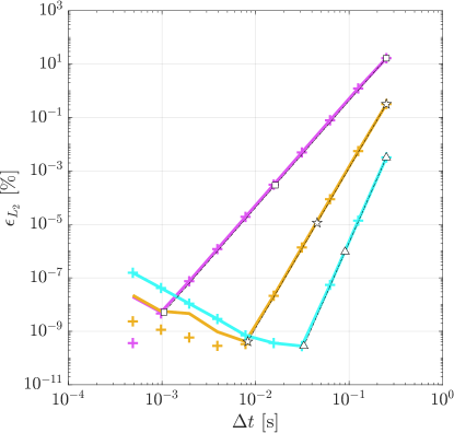
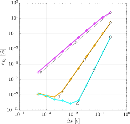
Figure 2: Acceleration error in the $L_{2}$-norm for the single degree of freedom system obtained by the algorithm for mixed-order Padé-based schemes in [9] with distinct roots. Left: $\rho_{\infty}=1$ ; Right: $\rho_{\infty}=0$. The dash-dotted lines indicate the optimal rates of convergence corresponding to slopes of 3 (right-pointing triangle), 4 (square), 5 (diamond), 6 (pentagram), 7 (hexagram), and 8 (upward-pointing triangle), respectively.

(a)

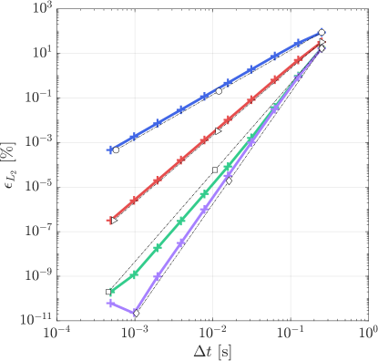
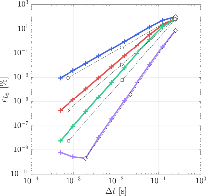
Figure 3: Acceleration error in the $L_{2}$-norm for the single degree of freedom system obtained by the algorithm for $M-$schemes in [34] with single multiple roots. Left: $\rho_{\infty}=1$ ; Right: $\rho_{\infty}=0$. The dash-dotted lines indicate the optimal rates of convergence corresponding to slopes of 2 (circle), 3 (right-pointing triangle), 4 (square) and 5 (diamond), respectively.

9.1.2 Nonlinear error analysis

To demonstrate the performance of the proposed algorithms on problems with strong nonlinearity, the nonlinear (SDOF) oscillating simple pendulum shown in Fig. 4 is considered here. The governing equation of motion is given as

$$\ddot{\theta}+\omega^{2}\sin\theta=0,\thinspace\thinspace\thinspace\theta_{0}=0\thinspace\mathrm{rad},\thinspace\thinspace\dot{\theta_{0}=1.999999238456499\thinspace\mathrm{rad/s}}\thinspace,$$

with $\omega=\sqrt{g/L}$ and the dimensionless case of $L=1,\thinspace g=1$ is used. The initial velocity is chosen such that the pendulum possesses the energy to almost reach its maximum position ($\theta_{\mathrm{max}}=\pm 179.9^{\circ}$) though not complete full rotations [29].

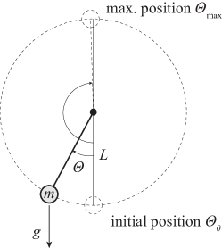
Figure 4: Nonlinear simple pendulum

The period of oscillation is approximately $T=33.712$ seconds, and the pendulum is simulated for two full periods. The errors shown in Fig. 5 and 6, for distinct root models and single root models, respectively, are based on the $L_{2}$-norm defined earlier in Eq. (89). The reference solution follows the exact solution provided in [29]. Once more for conciseness, only the error plots and convergence rates for accelerations are included here; the errors for displacements and velocities are of similar performance. It can be observed that the theoretical convergence rates are able to be met for this nonlinear problem. In Fig. 5a, the theoretical convergence rate is $2M$, however, there is an upper bound of 7 due to the interpolation scheme in use for state-space variables. For Fig. 5, the theoretical error rate is $2M-1$. For the $M$-schemes in Fig. 6, the theoretical error rate is $M$, and is achieved for all models. Numerical results using the $\rho_{\infty}$-Bathe model [42] overlap on the plots with the second-order model in this paper.

(a)

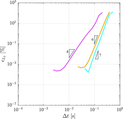
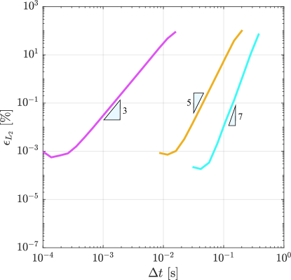
Figure 5: Acceleration error in the $L_{2}$-norm for the nonlinear oscillating simple pendulum obtained by the algorithm for mixed-order Padé-based schemes with distinct roots. Left: $\rho_{\infty}=1$ ; Right: $\rho_{\infty}=0$.

(a)

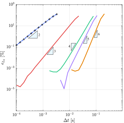
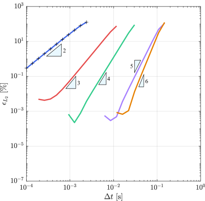
Figure 6: Acceleration error in the $L_{2}$-norm for the nonlinear simple pendulum obtained by the algorithm for $M-$schemes with single multiple roots. Left: $\rho_{\infty}=1$ ; Right: $\rho_{\infty}=0$.

Figure 7 presents the time-history for models using the distinct root algorithm presented in Table 1, with no numerical dissipation introduced ($\rho_{\infty}=1$). A large time step of $\Delta t=T/200=0.1686$ seconds is used to illustrate the difference in the responses obtained at various orders. As can be seen, during the second period of oscillation the (1,2) model erroneously completes a full revolution, whilst the (2,3) and (3,4) models are near indistinguishable from the reference solution. Figures 8 and 9 show the time history for single root algorithms presented in Table 2. The second-order model completes full revolutions, whilst the third-order model presents large period errors. For higher-order schemes, Fig 9 demonstrates how the period error reduces as the number of sub-steps increases, converging on the reference solution.

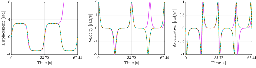
Figure 7: Time-history responses of the nonlinear oscillating pendulum using mixed-order Padé-based schemes, with $\Delta t=0.1686$ and $\rho_{\infty}=1$. Note that models relating to the (2,3) and (3,4) Padé expansions essentially overlap.

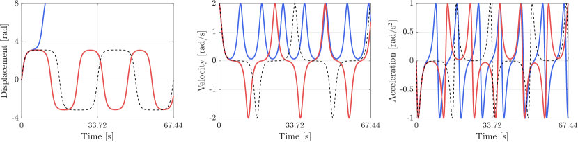
Figure 8: Time-history responses of the nonlinear oscillating pendulum using second- and third-order $M$-based schemes, with $\Delta t=0.1686$ and $\rho_{\infty}=1$.

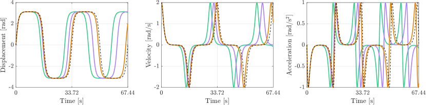
Figure 9: Time-history responses of the nonlinear oscillating pendulum using higher-order $M$-based schemes, with $\Delta t=0.1686$ and $\rho_{\infty}=1$.

Once more, it is observed from Figs. 5 and 6 that:

1. All schemes provide identical qualitative convergence as for linear problems.

2. All schemes converge at their optimal rates, up to a maximum of seven due to the Hermite interpolation polynomial used in the nonlinear solution algorithm.

3. For a given scheme, the error increases with decreasing $\rho_{\infty}$, i.e., increasing the amount of numerical damping. This difference is significant here due to the high nonlinearity of the problem.

4. The order of accuracy for schemes with single multiple roots is not affected by the value of $\rho_{\infty}$, while the order of accuracy for distinct roots cases will decrease by one if numerical damping is introduced.

5. High-order models achieve high levels of accuracy ($<10^{-3}\%$) using time steps several orders of magnitude larger than second- or third-order models.

9.2 Three-degree-of-freedom model problems

This section details the analysis of a linear and a nonlinear three-degree-of-freedom (3DOF) problem. The 3DOF problem is shown in Fig. 10. Each mass is taken to be $m_{1}=0$, $m_{2}=m_{3}=1$, and the system is initially at rest: $u_{2}(0)=\dot{u}_{2}(0)=u_{3}(0)=\dot{u}_{3}(0)=0$. The displacement of mass 1 is prescribed as $u_{1}=\sin(\omega_{p}t$) with $\omega_{p}=1.2$, corresponding to a period of vibration of $T_{p}=5.236$. Spring 1 is taken to be a stiff linear spring with coefficient $k_{1}=10^{7}$. The behaviour of Spring 2 is governed by the internal force function $N_{2}=N_{2}\left(\delta_{2}\right)$, a function of the elongation $\delta_{2}=u_{3}-u_{2}$. Following static condensation of the known displacement $u_{1}$, the equation of motion of the system as per Eq. (1) is expressed as:

$$\left[\begin{array}[]{cc}m_{2}&0\\ 0&m_{3}\end{array}\right]\left\{\begin{array}[]{c}\ddot{u}_{2}\\ \ddot{u}_{3}\end{array}\right\}+\left\{\begin{array}[]{c}k_{1}u_{2}-N_{2}\\ N_{2}\end{array}\right\}=\left\{\begin{array}[]{c}k_{1}u_{1}\\ 0\end{array}\right\},$$ (90)

which can be written in the form of Eq. (2) by taking as the mass, tangent damping and tangent stiffness, respectively:

$$\mathbf{M}=\left[\begin{array}[]{cc}m_{2}&0\\ 0&m_{3}\end{array}\right],\thinspace\thinspace\mathbf{C}_{n-1}=\mathbf{0},\thinspace\thinspace\mathbf{K}_{n-1}=\left[\begin{array}[]{cc}k_{1}+\frac{{\rm d}N_{2}}{{\rm d}\delta_{2}}&-\frac{{\rm d}N_{2}}{{\rm d}\delta_{2}}\\ -\frac{{\rm d}N_{2}}{{\rm d}\delta_{2}}&\frac{{\rm d}N_{2}}{{\rm d}\delta_{2}}\end{array}\right]\thinspace,$$ (91)

where the derivative ${\rm d}N_{2}/{\rm d}\delta_{2}$ is evaluated at $t_{n-1}$ in $\mathbf{K}_{n-1}$. The nonlinear force vector $\mathbf{f}(t)$ is given by

$$\mathbf{f}=\left\{\begin{array}[]{c}\left(k_{1}u_{1}+N_{2}\right)-\frac{{\rm d}N_{2}}{{\rm d}\delta_{2}}\delta_{2}\\ -N_{2}+\frac{{\rm d}N_{2}}{{\rm d}\delta_{2}}\delta_{2}\end{array}\right\}\thinspace.$$ (92)

The reaction force at $m_{1}$ is $R_{1}=m_{1}\ddot{u}_{1}+k_{1}(u_{1}-u_{2})$.

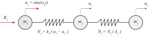
Figure 10: A three-degree-of-freedom model problem for linear and nonlinear analyses

9.2.1 Linear analysis

A linear analysis is performed to compare the proposed algorithm based on partial fraction decomposition with the original algorithms in [9, 34]. Here, the linear 3DOF problem studied in [36, 20] is considered, with $N_{2}=k_{2}\delta_{2}$, and $k_{2}=1$. As expected, $\mathbf{K}_{n-1}$ in Eq. (91) is constant-valued, and the force-vector from Eq. (92) is independent of unknown displacements and velocities. To suppress the high-frequency oscillations, $\rho_{\infty}=0$ is chosen. The time step size $\Delta t=0.14$ is selected as was used in [32]. The analysis is performed over an extended period of $t=5000$, approximately equivalent to $967\thinspace T_{p}$, to ensure a comprehensive analysis.

In the time-stepping schemes utilizing distinct roots, the acceleration responses of $m_{2}$, $m_{3}$, and the reaction force $R_{1}(t)$ are illustrated in Fig. 11. The solid lines represent results obtained with the proposed algorithm using partial fractions, while the plus markers with the same color denote results using the previous algorithm in [9]. The three columns of each figure show the responses at three different time intervals: $0\leq t\leq 10$ (left column), $500\leq t\leq 510$ (middle column), and $4990\leq t\leq 5000$ (right column). It is observed that both algorithms are numerically identical. Although the proposed method at order (1,2) exhibits a slight difference from the reference solution as time increases, the results converge to the reference solution as the order increases. At higher orders, specifically (2,3) and (3,4), the results overlap with the reference solution throughout the whole duration.

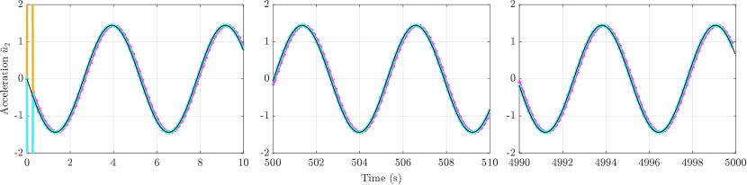
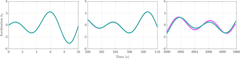
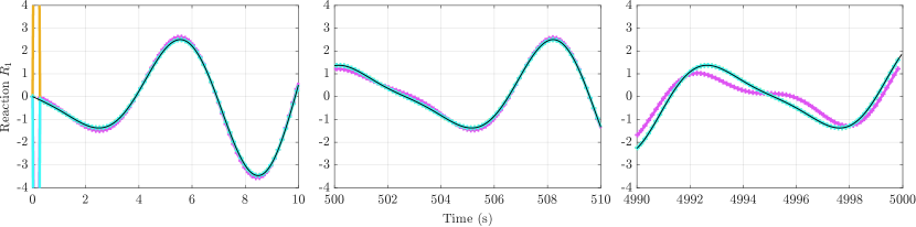
Figure 11: Acceleration responses of $m_{2}$ (top row), acceleration responses of $m_{3}$ (middle row), and reaction force response (bottom row) for distinct root cases during $0\leq t\leq 10$ (left column), $500\leq t\leq 510$ (middle column) and $4990\leq t\leq 5000$ (right column).

For the $M-$schemes in [34] with single multiple roots, the velocity and acceleration responses of $m_{2}$, $m_{3}$, and the reaction force $R_{1}(t)$ obtained with the present algorithm are plotted in Fig. 12. The solid lines represent results obtained with the proposed algorithm using partial fractions, and results from the previous algorithm in [34] are denoted by plus markers in corresponding colors. It is observed that the present algorithm and the algorithm in [34] yield numerically identical results. While all schemes exhibit satisfactory performance in the responses of $m_{2}$, significant deviations from the reference solutions are observed in the responses of $m_{3}$ and reaction force over time with the second-order scheme. Increasing the order leads to decreasing errors, and by fifth-order ($M=5$) the response is indistinguishable from the reference solution.

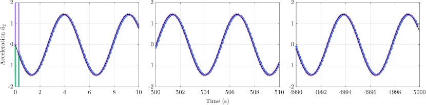
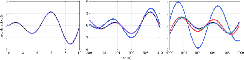
Figure 12: Acceleration responses of $m_{2}$ (top row), acceleration responses of $m_{3}$ (middle row), and reaction force response (bottom row) for the $M-$schemes with single multiple root during $0\leq t\leq 10$ (left column), $500\leq t\leq 510$ (middle column) and $4990\leq t\leq 5000$ (right column).

9.2.2 Nonlinear analysis

For the nonlinear case, Spring 2 is modelled by a nonlinear stiffening spring with internal force

$$N_{2}=k_{2}\sinh\delta_{2}\thinspace,$$ (93)

and $k_{2}=1$ is taken. The force-vector of Eq. (92) is nonlinear with respect to displacements.

Again, to suppress the high-frequency oscillations, $\rho_{\infty}=0$ is chosen and the analysis is performed over the extended period of $t=5000$. To demonstrate suitable numerical dissipation, a time step of $\Delta t=0.03$ is selected for all models. The elongation, internal force and stiffness of Spring 2 for $4950\leq t\leq 5000$ are shown in Fig. 13 for Padé-based schemes of order (1,2), (2,3), and (3,4), where all models effectively overlap for the duration of the test. The nonlinear stiffening spring ranges from 1 to approximately 18.32 in stiffness. Displacement response of masses $m_{2}$ and $m_{3}$ are presented in Fig. 14, with velocity responses shown in Fig. 15. Acceleration of each mass is presented in Fig. 16. The Padé-based models are of order $2M-1$ due to the use of numerical dissipation. The three columns of each figure show the responses at three different time intervals: $0\leq t\leq 5$ (left column), $500\leq t\leq 520$ (middle column), and $4980\leq t\leq 5000$ (right column). For displacement, velocity and acceleration, the Padé-based schemes tested overlap on the plots, converging on a solution for the entire duration.

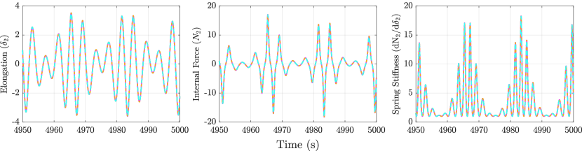
Figure 13: Response of nonlinear spring connecting masses $m_{2}$ and $m_{3}$ for the Padé-based schemes during $4950\leq t\leq 5000$

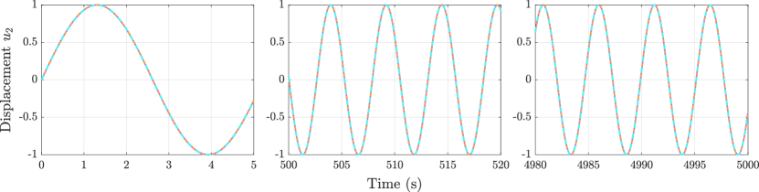
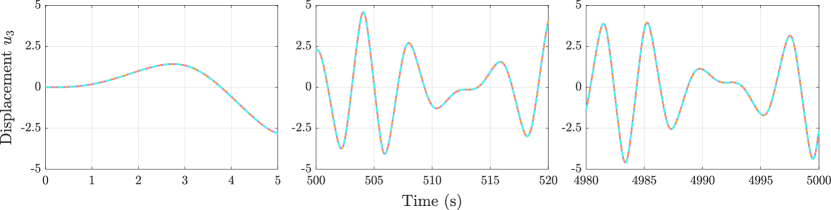
Figure 14: Displacement responses of $m_{2}$ (top row), and $m_{3}$ (bottom row), for the Padé-based schemes during $0\leq t\leq 5$ (left column), $500\leq t\leq 520$ (middle column) and $4980\leq t\leq 5000$ (right column).

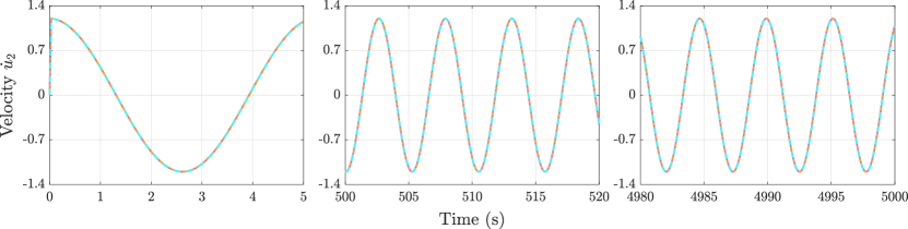
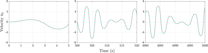
Figure 15: Velocity responses of $m_{2}$ (top row) and $m_{3}$ (bottom row), for the Padé-based schemes during $0\leq t\leq 5$ (left column), $500\leq t\leq 520$ (middle column) and $4980\leq t\leq 5000$ (right column).

Using $M$-based schemes (of accuracy $M$), Fig. 17 shows that the second- and third-order models deviate from high-order model solution as the simulation progresses, though all models of fourth-order or higher converge to the same solution as the high-order Padé-based models. Using $\rho_{\infty}=0$, all Padé-based and $M$-based schemes dampen the oscillations in the first time step.

Figure 18 presents the response of the HHT-$\alpha$ algorithm ($\alpha=-0.1$), with results using the second- and sixth-order $M$-schemes also shown for comparison. In addition to the large spurious oscillations produced for $m_{2}$, it is noted from that the HHT-$\alpha$ algorithm demonstrates poor accuracy in the response of $m_{3}$ over the duration of the simulation.

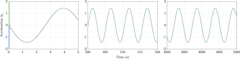
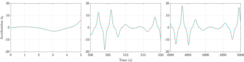
Figure 16: Acceleration response of $m_{2}$ (top row), and $m_{3}$ (bottom row), for the Padé-based schemes during $0\leq t\leq 5$ (left column), $500\leq t\leq 520$ (middle column) and $4980\leq t\leq 5000$ (right column).

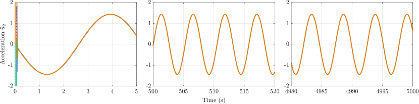
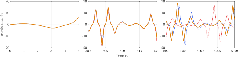
Figure 17: Acceleration responses of $m_{2}$ (top row), and $m_{3}$ (bottom row), for the $M-$schemes with single multiple root during $0\leq t\leq 5$ (left column), $500\leq t\leq 520$ (middle column) and $4980\leq t\leq 5000$ (right column).

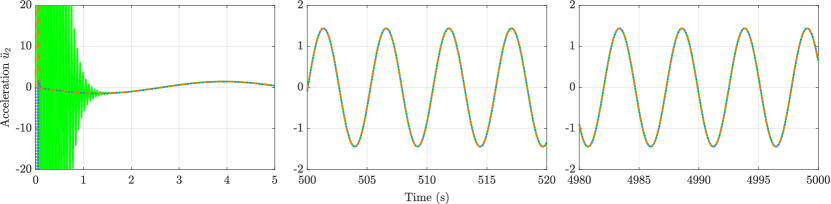
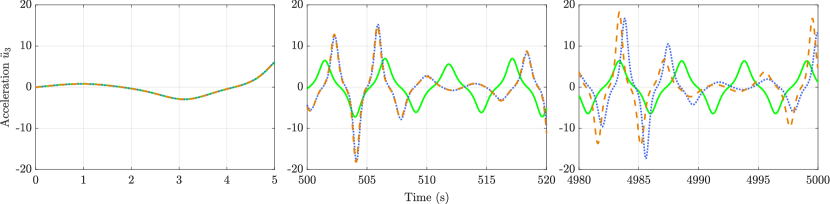
Figure 18: Acceleration responses of $m_{2}$ (top row), and $m_{3}$ (bottom row), for the HHT-$\alpha$ method ($\alpha=-0.1$), and second- and sixth-order $M-$schemes with single multiple root for comparison; for time durations $0\leq t\leq 5$ (left column), $500\leq t\leq 520$ (middle column) and $4980\leq t\leq 5000$ (right column).

9.3 One-dimensional wave propagation in a prismatic rod

A prismatic rod subjected to a triangular impulse of loading, as illustrated in Fig. 19, is frequently used to evaluate the performance of time integration methods. Most studies are limited to displacement and velocity. In this section, the acceleration response is also investigated. A consistent set of units is used: the length $L$ and cross-section area $A$ of the rod are chosen as unit values, i.e., $L\,{=}\,1$ and $A\,{=}\,1$. The left end of the rod is fixed. The triangular impulse force $F(t)$ is applied at the right (free) end with a peak value of $0.0001$ reached at $t=0.2$ (Fig. 19b). The material properties are chosen as: Young’s modulus $E\,{=}\,1$, Poisson’s ratio $\nu\,{=}\,0$, and mass density $\rho\,{=}\,1$. The d’Alembert’s solution of wave equation is derived and used as the exact solution in the following investigation. The responses at two specific points marked by the dots in Fig. 19a), Point A at the loaded (right) end and Point B at the midpoint, are considered.

The spatial discretization of the prismatic rod consists of $2{,}000$ linear finite elements uniformly spaced along the length (element size of $\Delta x=5\times 10^{-4}$). The Courant-Friedrichs-Lewy (CFL) number is calculated as $\mathrm{CFL}=c\,(\Delta t/\Delta x)$ with the longitudinal wave speed defined by $c=\sqrt{E/\rho}=1$. During each line segment of the triangle impulse, i.e., $t\in[0,0.2]$ and $t\in[0.2,$0.4], the wave propagates through $400$ elements. The frequency spectrum of the loading is shown in Fig. 19c. The value is negligible beyond the frequency of $20$, which is considered as the maximum frequency of interest. At this frequency, the wavelength is $0.05$, i.e. about the length of $100$ elements. The mesh is considered to be very fine for earthquake engineering applications.

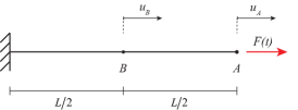
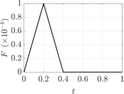
a) b) c)

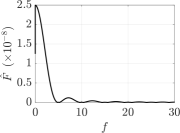
Figure 19: A prismatic rod subjected to triangular impulse: a) Geometry and boundary conditions; b) Excitation signal in the time domain; c) Excitation signal in the frequency domain.

For comparison, the HHT-$\alpha$ method and the explicit second-order central-difference time integration method built in the commercial finite element package Abaqus are also employed to analyze this wave propagation problem. For the HHT-$\alpha$ method, the parameters are chosen as $\alpha=-0.1$ and $\mathrm{CFL}=1$. For the explicit method, automatic time-stepping in Abaqus is used which yields a $\mathrm{CFL}=0.99$. All time integration methods perform very well in predicting the displacement and velocity responses. For brevity, Fig. 20 only shows the velocity responses of a few selected schemes.

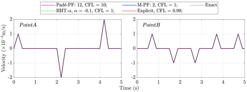
Figure 20: Velocity response of the rod.

The acceleration responses reveal a notable difference in the performance of the time integration methods. The results of the HHT-$\alpha$ method and the explicit method of Abaqus are plotted in Fig. 21 and Fig. 22, respectively. Significant spurious high-frequency oscillations are observed. The explicit method (Fig. 22) leads to noticeably stronger oscillations than the implicit method does (Fig. 21).

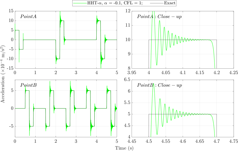
Figure 21: Acceleration response of the prismatic rod obtained with HHT-$\alpha$ method in Abaqus.

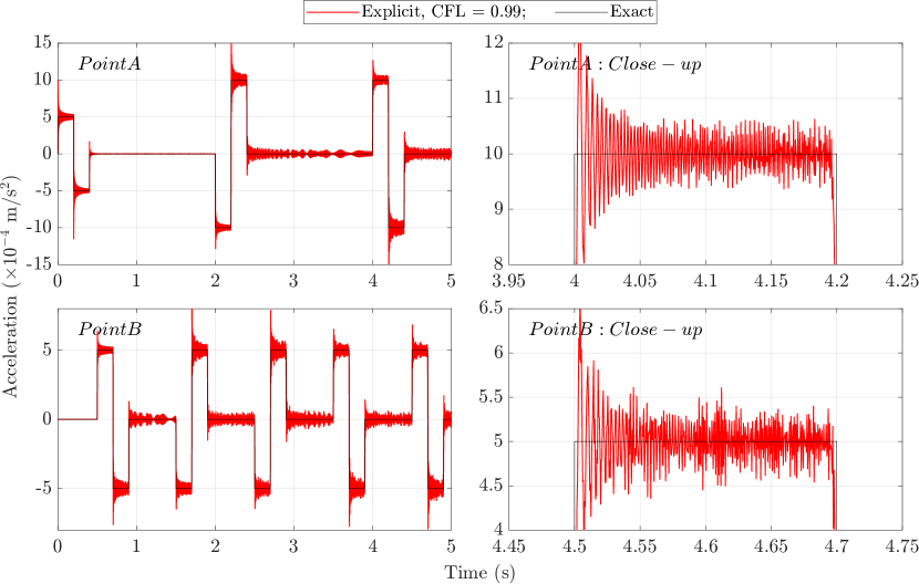
Figure 22: Acceleration response of the prismatic rod obtained with explicit method in Abaqus.

The Bathe method [40, 8] has been reported to have better performance than the HHT-$\alpha$ method in suppressing spurious oscillations. It is shown in [34] and verified for this example that the $M=2$ composite scheme is numerically equivalent to the second-order $\rho_{\infty}$-Bathe method. This scheme is considered with the parameters $\rho_{\infty}=0$ and $\mathrm{CFL}=1$. Using the proposed algorithm for single multiple roots, the acceleration responses are obtained and shown in Fig. 23. The spurious oscillations observed in the HHT-$\alpha$ and explicit methods are largely suppressed. At Point A, overshoots appear within the duration of the triangle impulse.

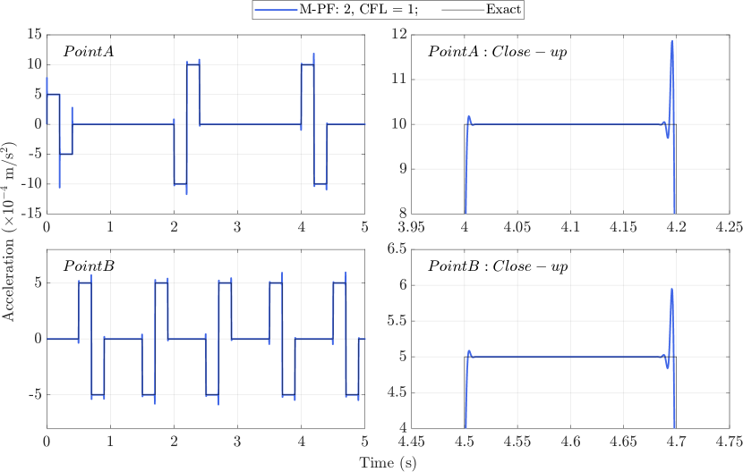
Figure 23: Acceleration response of the prismatic rod obtained with the second-order $M=2$ cases.

The high-order schemes from [34] are considered with the parameter $\rho_{\infty}=0$. The proposed algorithm for the case of single multiple roots is applied. The CFL numbers are selected according to the order of the schemes by following the recommendation in [34] as: $\mathrm{CFL}=5$ for $M=3$ (third-order), $\mathrm{CFL}=8$ for $M=4$ (fourth-order) and $\mathrm{CFL}=12$ for $M=5$ (fifth-order). The acceleration responses are plotted in Fig. 24. It can be observed that the spurious oscillations, including the overshoots at Point A, are effectively suppressed here.

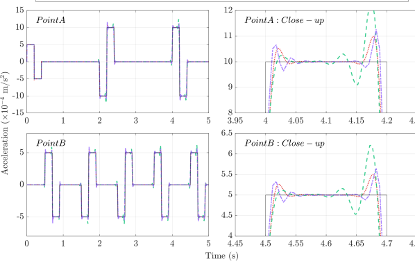
Figure 24: Acceleration response of the prismatic rod obtained with the single multiple roots cases.

The high-order schemes based on the Padé expansion of the matrix exponential in [9] are considered by applying the current proposed algorithm for distinct roots. Again, the parameter $\rho_{\infty}=0$ is used. The CFL numbers are chosen as $\mathrm{CFL}=10$ for the third-order scheme (PadéPF:12), $\mathrm{CFL}=20$ for the fifth-order scheme (PadéPF:23), and $\mathrm{CFL}=30$ for the seventh-order scheme (PadéPF:34). The acceleration responses are shown in Fig. 25. It is observed that the spurious oscillations have been effectively suppressed. The overshoots are also smaller than those in other schemes.

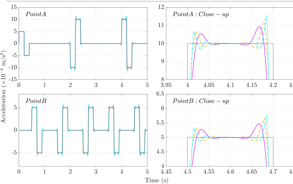
Figure 25: Acceleration response of the prismatic rod obtained with distinct roots cases.

9.4 Two-dimensional wave propagation in a semi-infinite elastic plane - Lamb problem

Lamb’s problem with a vertical point load is examined under plain strain conditions in this section. This a typical example of wave propagation in earthquake engineering where the acceleration response is of practical importance in a seismic design. As depicted in Fig. 26, considering symmetry, only the right side relative to the point load $F(t)$ is considered using the boundary conditions shown. The investigation is conducted within a square domain of dimension $l\times l$. The material parameters of the linear elastic half-plane are chosen the same as in [7] and [8]: Young’s modulus $E=18.77\times 10^{9}\,\mathrm{\,Pa},$ Poisson’s ratio $\nu=0.25$, and mass density $\rho=2{,}200\,\mathrm{\,kg/m^{3}}$. Accordingly, the P-wave, S-wave and Rayleigh-wave speeds are equal to $c_{p}=3{,}200\,\,\mathrm{m/s}$, $c_{s}=1{,}847.5\,\mathrm{\,m/s}$, and $c_{R}=1{,}698.6\,\,\mathrm{m/s}$, respectively. The time history of the point load is obtained by integrating the series of step functions in [8] as

$$F(t)=\begin{cases}2\times 10^{6}t\,\mathrm{N}&0\leq t<0.05\,\mathrm{s}\\ 10^{5}-4\times 10^{6}\times(t-0.05)\,\mathrm{N}&0.05\,\mathrm{s}\leq t<0.1\,\mathrm{s}\\ -10^{5}+2\times 10^{6}\times(t-0.1)\,\mathrm{N}&0.1\,\mathrm{s}\leq t\leq 0.15\,\mathrm{s}\end{cases}$$

as shown in Fig. 26b. Reference solutions are given in [8] for the displacements at the two observation points, $P_{1}\,(640,2{,}800)$ and $P_{2}\,(1{,}280,2{,}800)$, indicated in Fig. 26a. Under the present loading case, these reference solutions correspond to the solutions of the velocity responses.

To mitigate the effect of wave reflections from the boundaries, the length of the extended square domain is chosen as $l=2{,}800\,\mathrm{\,m}$, which is large enough to ensure no reflections from the artificially fixed boundaries reach the observation points within $1\,\,\mathrm{s}$. The domain is discretized into a uniform mesh consisting of $2{,}800\times 2{,}800$ linear finite elements, leading to a total of $15{,}682{,}799$ degrees of freedom. Each element is a square with a side length $\Delta x=1\,\mathrm{m}$. The CFL number is calculated as $\mathrm{CFL}=c_{p}\Delta t/\Delta x$. The mesh is sufficiently fine for earthquake engineering applications. During one line segment of the loading, i.e. $0.05\,\mathrm{s}$, the Rayleigh-wave travels about $85\,\mathrm{m}$, i.e. 85 elements. The frequency spectrum of the loading is plotted in Fig. 26b. Considering the maximum frequency of interest as $75\,\mathrm{Hz}$, the Rayleigh wavelength is about $22.6\,\mathrm{m}$.

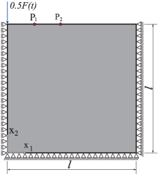
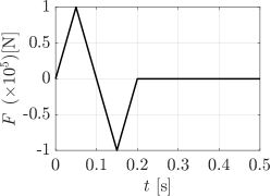
a) b) c)

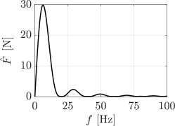
Figure 26: A semi-infinite elastic domain in plane strain conditions: a) Geometry and boundary conditions; b) Excitation signal in the time domain; c) Excitation signal in the frequency domain.

The commercial finite element package Abaqus is first employed to analyze this wave propagation problem. The velocity and acceleration responses obtained using the HHT-$\alpha$ method with $\alpha=-0.1$ and $\mathrm{CFL}=1$ and the explicit method with $\mathrm{CFL}=0.93$ are shown in Figs. 27 and 28, respectively. Note that the vertical response is larger than the horizontal response, and different scales are used for each in the plots. Some spurious high-frequency oscillations are observed in the velocity responses. The explicit method exhibits stronger oscillations than the implicit method, especially after the waves have passed. The acceleration responses from both explicit and implicit methods are heavily polluted by the high-frequency oscillations to the extent that the results are not directly usable.

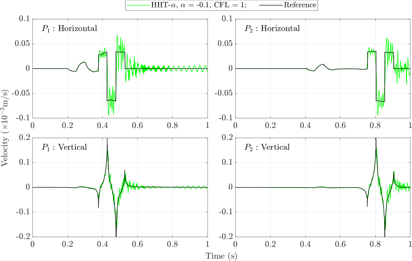
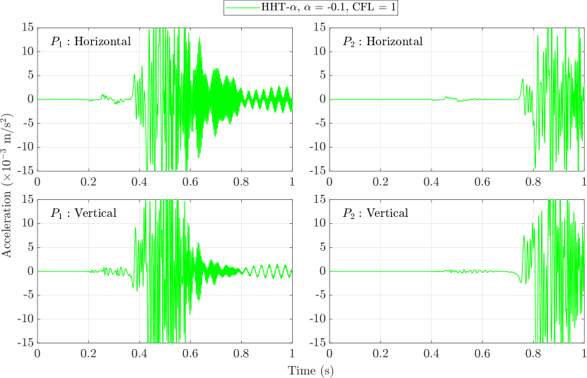
Figure 27: Velocity and acceleration response of the Lamb problem obtained with the HHT-$\alpha$ method in Abaqus.

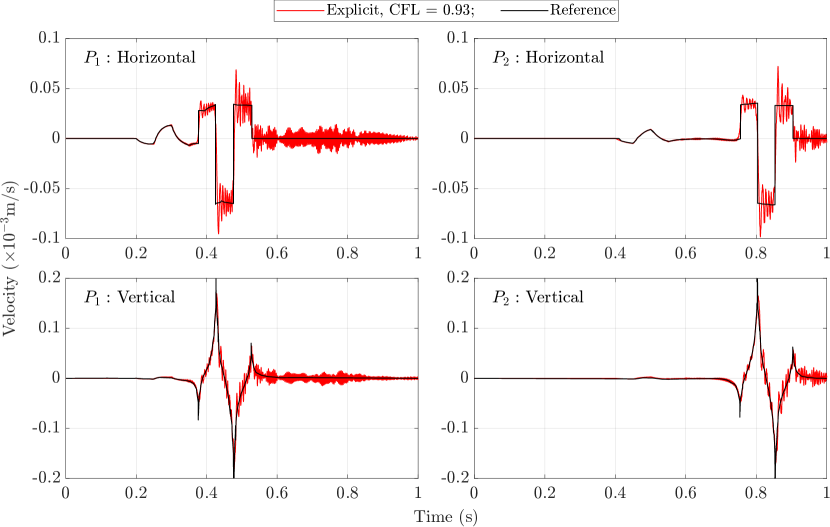
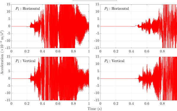
Figure 28: Velocity and acceleration response of the Lamb problem obtained with the explicit method in Abaqus.

The $M=2$ composite scheme, which is numerically equivalent to the second-order $\rho_{\infty}$-Bathe method, is considered with the parameter $\rho_{\infty}=0$. The velocity and acceleration responses obtained using the proposed algorithm for single multiple roots are shown in Fig. 29 (denoted as "M-PF: 2"). The spurious high-frequency oscillations are significantly smaller in the velocity responses than those observed in the results of HHT-$\alpha$ and explicit methods. Noticeable oscillations still exist in the acceleration responses.

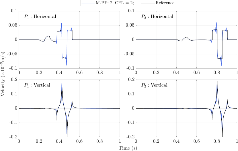
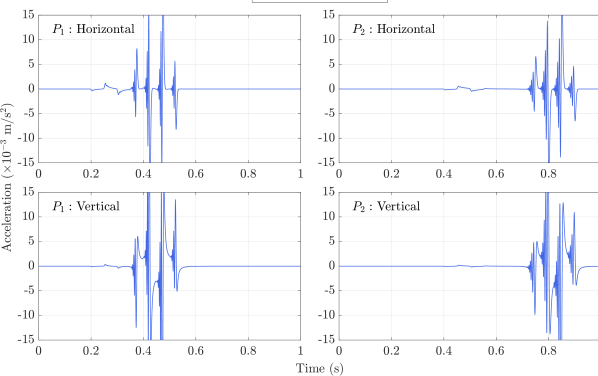
Figure 29: Velocity and acceleration response of the Lamb problem obtained by the $M=2$ composite scheme with single multiple roots.

The proposed algorithm is then applied with the high-order composite schemes of orders $M=3$ and $4$. The parameter $\rho_{\infty}=0$ is used. The CFL numbers are selected as $\mathrm{CFL}=5$ for $M=3$ and $\mathrm{CFL}=8$ for $M=4$ schemes according to the recommendation outlined in [34]. The proposed algorithm with single multiple roots is applied. The velocity and acceleration responses are shown in Fig. 30. Good agreement with the reference solution is observed for velocity responses. Spurious oscillations observed in the acceleration responses predicted by the second-order schemes are largely suppressed here. The results obtained with orders $M=3$ and $4$ are very similar.

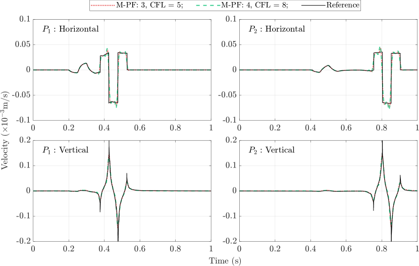
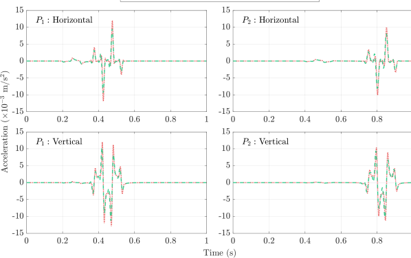
Figure 30: Velocity and acceleration response of the Lamb problem obtained with the $M=3$ and $4$ composite scheme with single multiple roots.

The proposed algorithm for the distinct roots case is applied with the Padé-expansion based schemes in [9]. The parameter $\rho_{\infty}=0$ is used. The velocity and acceleration response are plotted in Fig. 31. The CFL numbers are chosen as $\mathrm{CFL}=10$ for the third-order scheme (PadéPF:12) and $\mathrm{CFL}=20$ for the fifth-order scheme (PadéPF:23). Again, good agreement with the reference solution of velocity is observed. No significant spurious oscillations exist in both velocity and acceleration responses. The results of both high-order models are close to each other and also to the results obtained with the high-order single multiple root composite schemes in Fig. 30.

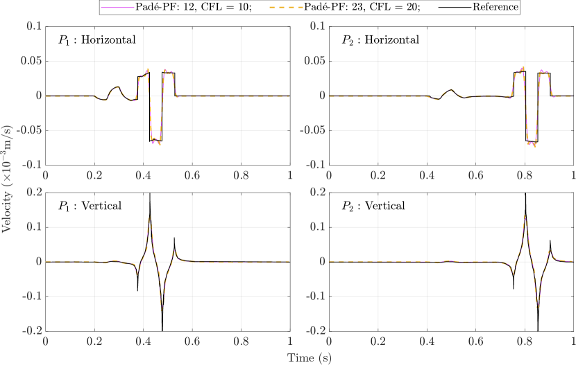
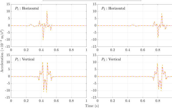
Figure 31: Velocity and acceleration response of the Lamb problem obtained by distinct roots cases.

10 Conclusions

A new algorithm for a family of high-order implicit time integration schemes based on the rational approximation of matrix exponential is proposed. Compared with our previous works, the new algorithm removes the need for the factorization of the mass matrix and is particularly advantages for nonlinear problems. A new tecnique to compute the acceleration without additional equation solutions is proposed. The acceleration is obtained at the same order of accuracy as the displacement. As only vector operations are used, the additional computational cost is minimal.

It is observed from the numerical examples that the implicit HHT-$\alpha$ method, explicit second-order central-difference method, and implicit second-order composite methods may heavily pollute the acceleration responses for some wave propagation problems. The high-order schemes are highly effective in suppressing the spurious high-frequency oscillations when the order is equal to or higher than three. For nonlinear problems, the proposed algorithms show the same convergence rates for linear problems and very high accuracy.

Appendix A Illustrative examples for determining coefficients

An important aspect of the algorithm presented in this work is initializing the coefficients used in the partial fraction decomposition of the matrix exponential, and therefore executing the numerical integration to the desired degree of accuracy. This Appendix provides sample MATLAB code for initializing the scheme for two cases: 1). distinct roots, and 2). single multiple root. In both cases, the algorithms require only the order of the numerical scheme $M$ and the user-defined parameter $\rho_{\infty}\in[0,1]$ to be defined. Examples of the coefficients determined for third-order ($M=3$) schemes with arbitrarily chosen $\rho_{\infty}=0.125$ are provided for each of the two cases.

Distinct roots

Figure 32 presents MATLAB code that executes the algorithm required to determine the roots $r_{i}$, the coefficients $p_{\mathrm{L}i}$, $a_{i}$, and matrix $\mathbf{c}$ required to initialize the time-stepping scheme for the case of distinct roots, and therefore be able to solve Eq. (45). The Padé-expansion based scheme with order $(L=2,\,M=3)$ is considered as an example, and the spectral radius $\rho_{\infty}=0.125$ is used (which has fifth-order accuracy when numerical dissipation is introduced). This is run by executing $\texttt{InitSchemePadePF(3, 0.125)}.$

function [rho, plr, rs, a, cfr] = function [rho, plr, rs, a, cfr] = InitSchemePadePF(M,rhoInfty,pf)

[pcoe, qcoe, rs] = PadeExpansion(M,rhoInfty);

rho = pcoe(end)/qcoe(end);

plcoe = pcoe(1:end-1) - rho*qcoe(1:end-1);

a = polyPartialFraction(qcoe, rs);

plr = plcoe*reshape(rs,1,[]).^((0:M-1)’);

cf = TimeIntgCoeffForce(pcoe,qcoe,pf);

cfr = cf*reshape(rs,1,[]).^((0:M-1)’);

Figure 32: MATLAB code for initializing the time-stepping scheme for case of single multiple root

The first line uses a function PadeExpansion to find coefficients of the polynomials in Eq. (27). This function is provided in Fig. 33.

function [pcoe, qcoe, r] = PadeExpansion(M,rhoInfty)

L = M-1;

[p1, q1] = PadeCoeff(M, M);

[p2, q2] = PadeCoeff(M, L);

pcoe = rhoInfty*p1 + (1-rhoInfty)*[p2 zeros(M-L)];

qcoe = rhoInfty*q1 + (1-rhoInfty)*q2;

r = roots(fliplr(qcoe));

r(imag(r)<-1.d-6) = [];

[~, idx] = sort(imag(r));

r = r(idx);

end

function [p, q] = PadeCoeff(M,L)

fc = @(x) factorial(x);

ii=0:L;

p=(fc(M+L-ii))./(fc(ii).*fc(L-ii));

ii=0:M;

q=(fc(M+L-ii)).*((-1).^ii)./(fc(ii).*fc(M-ii))*fc(M)/fc(L);

end

Figure 33: MATLAB function to determine the coefficients of the Padé expansion for case of distinct roots, and find the roots of $Q(\mathbf{A})$.

Following [9], each polynomial is defined in the following mixed form

$$\mathbf{P} =\rho_{\infty}\mathbf{P}_{M/M}+\left(1-\rho_{\infty}\right)\mathbf{P}_{L/M}\,,$$ (94)

$$\mathbf{Q} =\rho_{\infty}\mathbf{Q}_{M/M}+\left(1-\rho_{\infty}\right)\mathbf{Q}_{L/M}\,,$$ (95)

where the coefficients are determined through use of

$$\mathbf{P}_{L/M} =\sum_{i=0}^{L}\frac{\left(M+L-i\right)!}{i!\left(L-i\right)!}\mathbf{A}^{i}\,,$$ (96)

$$\mathbf{Q}_{L/M} =\frac{M!}{L!}\sum_{i=0}^{M}\frac{\left(M+L-i\right)!}{i!\left(M-i\right)!}\left(-\mathbf{A}\right)^{i}\,.$$ (97)

In the current work, the partial fraction expansion uses $L=M-1$, and for the demonstrative example case $M=3$ and $\rho_{\infty}=0.125$, the coefficients of the following polynomials

$$\mathbf{P}=67.5\mathbf{I}+28\mathbf{A}+4.125\mathbf{A}^{2}+0.125\mathbf{A}^{3}\,,$$ (98)

$$\mathbf{Q}=67.5\mathbf{I}-39\mathbf{A}+9.375\mathbf{A}^{2}-1\mathbf{A}^{3}\,.$$ (99)

are returned in vectors pcoe, qcoe. Therefore, the spectral radius is given by $\rho=p_{M}/q_{M}=-0.125$. The polynomial $\mathbf{Q}$ in Eq. (99) has one real root and two complex-conjugate roots which may be solved to be:

$$r_{1}=3.7821,\ \ r_{2,3}=2.7964\pm 3.1665\ \mathrm{i}\,,$$ (100)

stored in rs. The coefficients of the polynomials $P_{\mathrm{L}}(r_{i})$ in Eq. (37) are collected in plcoe by use of Eq. (28):

$$P_{\mathrm{L}}(r_{i})=75.9375+23.6250r_{i}+5.2969r_{i}^{2}\,.$$ (101)

Next, the function polyPartialFraction determines parameters $a_{i}$ for each root using Eq. (34), returning for the example case:

$$a_{1}=0.909,\ \ a_{2}=a_{3}=-0.0455+0.0142\mathrm{i}\,.$$ (102)

Finally, by employing the function timeIntgCoeffForce in Fig. 35 the coefficient matrix $\mathbf{c}$ is found. For the example case, Eqs. (23) and (24), matrix polynomials $\mathbf{C}_{k}$ are obtained as

$$C_{k}(\mathbf{A})=\left[\begin{array}[]{c}67.5\mathbf{I}-5.25\mathbf{A}+1.125\mathbf{A}^{2}\\ -0.5625\mathbf{A}+0.4375\mathbf{A}^{2}\\ 5.625\mathbf{I}-0.4375\mathbf{A}+0.2812\mathbf{A}^{2}\\ -0.8438\mathbf{A}+0.1094\mathbf{A}^{2}\end{array}\right]\,.$$ (103)

and, therefore, the coefficient matrix stored as:

$$\mathbf{c}=\left[\begin{array}[]{ccc}67.5&-5.25&1.125\\ 0&-0.5625&0.4375\\ 5.625&-0.4375&0.2812\\ 0&-0.8438&0.1094\end{array}\right]\,.$$ (104)

The function InitSchemePadePF(3, 0.125) in Fig. 34 then returns the parameter $\rho=-0.125$, as well as the coefficients $p_{\mathrm{L}i}$ (Eq. (101)), the distinct roots $r_{i}$ (Eq. (100)), the coefficients $a_{i}$ (Eq. (102)) and the matrix $\mathbf{c}$ (Eq. (104)), as required.

Single multiple root

Sample MATLAB code to determine the root $r$, the coefficients $p_{\mathrm{r}i}$, and matrix $\mathbf{c}_{\mathrm{r}}$ required to initialize the time-stepping scheme for the case of single multiple roots is provided in Fig. 34. Note that the function shiftPolyCoefficients was provided earlier in Fig. 1.

function [r, prcoe, cfr] = InitSchemeRhoPF(M, rhoInfty, pf)

r = MschemeRoot(M, rhoInfty);

pcoe = pCoefficients(M, r);

prcoe = shiftPolyCoefficients(pcoe,r);

qrcoe = [zeros(1,M) 1];

qcoe = shiftPolyCoefficents(qrcoe,r);

cf = TimeIntgCoeffForce(pcoe,qcoe,pf);

cfr = shiftPolyCoefficients(cf,r);

Figure 34: MATLAB code for initializing the time-stepping scheme for case of single multiple root

Consider the case of finding the root and coefficients for a third-order scheme ($M=3$) with spectral radius $\rho_{\infty}=0.125$ required to implement the final time-stepping equation for the case of single-multiple roots as given in Eq. (63). This is equivalent to executing the function InitSchemeRhoPF(3, 0.125) using Fig. 34. The first step uses the function MschemeRoot (provided in [34]) to solve for the single multiple root $r$. The expansion of polynomial $p_{M}(r)$ for the third-order scheme ($M=3$) is:

$$p_{M}(r)=-1+3r-\frac{3}{2}r^{2}+\frac{1}{8}r^{3}=\pm\rho_{\infty}\,,$$ (105)

where, for $M=3$ the RHS is set equal to $-\rho_{\infty}$ (see [34])

$$-1+3r-\frac{3}{2}r^{2}+\frac{1}{6}r^{3}=-0.125\,,$$ (106)

which, by solving this cubic equation and testing the three roots by considering the stability of the schemes, the root

$$r=2.3917$$ (107)

is selected. Using the function pCoefficients (provided in [34]) with the newly found root $r=2.3917$, the polynomial $P(\mathbf{A})$ can be given as follows

$$P(\mathbf{A})=13.6802\mathbf{I}-3.4798\mathbf{A}-3.1449\mathbf{A}^{2}-0.125\mathbf{A}^{3}\,.$$ (108)

with coefficients stored in pcoe. Through use of Eq. (52), the algorithm shiftPolyCoefficients transforms Eq. (108) to a polynomial in terms of the matrix $\mathbf{A}_{r}$

$$P_{\mathrm{r}}(\mathbf{A}_{\mathrm{r}}) =13.6802\mathbf{I}-3.4798(2.3917\thinspace\mathbf{I}-\textbf{A}_{\mathrm{r}})-3.1449(2.3917\thinspace\mathbf{I}-\mathbf{A}_{\mathrm{r}})^{2}-0.125(2.3917\thinspace\mathbf{I}-\mathbf{A}_{\mathrm{r}})^{3}$$

$$=-14.3410\mathbf{I}+20.6678\mathbf{A}_{\mathrm{r}}-4.0418\mathbf{A}_{\mathrm{r}}^{2}+0.125\mathbf{A}_{r}^{3}\,,$$ (109)

and returns the coefficients in the vector prcoe. The denominator of the expansion in Eq. (50) is equivalent to $\mathbf{A}_{r}^{M}$, and therefore all coefficients of polynomial $\mathbf{Q}_{r}$ are zero except the term of order $M$ as defined for the variable qrcoe. Coefficients of $\mathbf{Q}$ are found using the shifting algorithm shiftPolyCoefficients.

The MATLAB function TimeIntgCoeffForce for determining the coefficient matrix related to the expression in Eq. (110) is provided in Fig. 35.

function [C] = TimeIntgCoeffForce(p, q, pf)

M = length(q) - 1;

tmp = p - q;

C = zeros(pf+1,M);

C(1,:) = tmp(2:end); %ltx order reduced by one {A}^{-1}\left({P}-{Q}\right)

for k = 1:pf

tmp = ((-1/2)^k)*(p-((-1)^k)*q); %ltx order of $C_{k-1}$ is lower than $q$ by one

tmp(1:M) = tmp(1:M) + k*C(k,:);

C(k+1,:) = tmp(2:end);

end

Figure 35: MATLAB function to determine the coefficients required to integrate the non-homogeneous term $C_{k}(\mathbf{A})$.

Following Eqs. (23) and Eqs. (24), the matrix polynomials $\mathbf{C}_{k}$ can be obtained as

$$C_{k}(\mathbf{A})=\left[\begin{array}[]{c}13.6802\mathbf{I}-10.3199\mathbf{A}+0.875\mathbf{A}^{2}\\ -1.14\mathbf{A}+0.5625\mathbf{A}^{2}\\ 1.14\mathbf{I}-1.455\mathbf{A}+0.2187\mathbf{A}^{2}\\ -1.7849\mathbf{I}+0.1525\mathbf{A}+0.1406\mathbf{A}^{2}\end{array}\right]\,,$$ (110)

which once more, by employing Eq. (52), are re-written in terms of $\mathbf{A}_{\mathrm{r}}$:

$$C_{\mathrm{r}k}(\mathbf{A}_{\mathrm{r}}) =\left[\begin{array}[]{c}13.6802\mathbf{I}-10.3199(2.3917\thinspace\mathbf{I}-\mathbf{A}_{\mathrm{r}})+0.875(2.3917\thinspace\mathbf{I}-\mathbf{A}_{\mathrm{r}})^{2}\\ -1.14(2.3917\thinspace\mathbf{I}-\mathbf{A}_{\mathrm{r}})+0.5625(2.3917\thinspace\mathbf{I}-\mathbf{A}_{\mathrm{r}})^{2}\\ 1.14\mathbf{I}-1.455(2.3917\thinspace\mathbf{I}-\mathbf{A}_{\mathrm{r}})+0.2187(2.3917\thinspace\mathbf{I}-\mathbf{A}_{\mathrm{r}})^{2}\\ -1.7849\mathbf{I}+0.1525(2.3917\thinspace\mathbf{I}-\mathbf{A}_{\mathrm{r}})+0.1406(2.3917\thinspace\mathbf{I}-\mathbf{A}_{\mathrm{r}})^{2}\end{array}\right]$$ (115)

$$=\left[\begin{array}[]{c}-5.9963\mathbf{I}+6.1345\mathbf{A}+0.875\mathbf{A}^{2}\\ 0.491\mathbf{I}-1.5506\mathbf{A}+0.5625\mathbf{A}^{2}\\ -1.0885\mathbf{I}+0.4086\mathbf{A}+0.2187\mathbf{A}^{2}\\ -0.6158\mathbf{I}-0.8251\mathbf{A}+0.1406\mathbf{A}^{2}\end{array}\right]\,,$$ (120)

and, consequently, the coefficient matrix is stored as

$$\mathbf{c}_{\mathrm{r}}=\left[\begin{array}[]{ccc}-5.9963&6.1345&0.8750\\ 0.4910&-1.5506&0.5625\\ -1.0885&0.4086&0.2187\\ -0.6158&-0.8251&0.1406\end{array}\right]\,.$$ (121)

The function InitSchemeRhoPF(3, 0.125) in Fig. 34 then returns the root $r$ in Eq. (107), the coefficients $p_{\mathrm{r}i}$ of Eq. (109), and the coefficient matrix $\mathbf{c}_{\mathrm{r}}$ in Eq. (121), as required.

Appendix B Sample MATLAB code for linear time-stepping solution algorithms

Figure 36 and Figure 37 provide sample MATLAB code for executing the algorithms presented in this work for linear problems. These can be simply extended to nonlinear problems by introducing an iterative solution procedure as presented in Tables 1 and 2. Note that the functions InitSchemePadePF and InitSchemeRhoPF used to initialize the coefficients required for the time-stepping solution for each procedure were provided in Fig. 32 and Fig. 34. The function lu is used in Fig. 37 for the solution of complex equations since it is found to be faster than the decomposition function in MATLAB 2023b.

function [RespHist] = TimeSolverPF(porder,signal,ns,dt,K,M,C,F,MLumped,u0,v0)

p = mod(porder(1),10);

rhoInfty = porder(2);

nCmplx = floor(p/2);

nReal = mod(p,2);

pf = min(p+1,size(cfr,1));

[rho, plr, rs, a, cfr] = InitSchemePadePF(p,rhoInfty,pf);

s = forceSamplingPoints(pf+0);

Tcfr = transMtxPointsToPoly(s, pf)*cfr(1:pf,:);

if nReal > 0

r = rs(1);

dKd1 = decomposition(sparse((r*r)*M + r*C + K));

end

if nCmplx > 0

L = cell(nCmplx,1); U = L; LUp = L; LUq = L;

for ic = 1:nCmplx

r = rs(ic+nReal);

[L{ic},U{ic},LUp{ic},LUq{ic}] = lu(sparse((r*r)*M + r*C + K),’vector’);

end

end

n = size(K,1);

tm = 0; z0 = [v0; u0]; % Initial conditions

an = (F*signal(0)+ftmp)./MLumped;

for is= 1:ns-1

ts = tm + dt*s;

Fp = F.*reshape(signal(ts), 1, []);

tm = tm + dt;

z = rho*z0;

Az1 = rho*Az1;

if nReal > 0

r = real(rs(1));

g = real(plr(1))*z0;

fri = Fp*(real(Tcfr(:,1)));

ftmp = dKd1\(r*(M*g(1:n)) - K*g(n+1:end) + r*fri);

y = [ftmp ; (ftmp+g(n+1:end))/r];

z = z + real(a(1))*y;

ftmp = r*y(1:n) - ( g(1:n) + fri./MLumped );

Az1 = Az1 + real(a(1))*ftmp;

end

Figure 36: MATLAB function to solve the time-stepping equation for case of distinct roots.

if nCmplx > 0

for ic = 1:nCmplx

r = rs(ic+nReal);

cg = plr(ic+nReal)*z0;

cfri = Fp*(Tcfr(:,ic+nReal));

ctmp = plr(ic+nReal)*(r*(M*z0(1:n)) - K*z0(n+1:end)) + r*cfri;

tmp(LUp{ic},:) = U{ic}\(L{ic}\ctmp(LUq{ic},:));

y = [tmp; (tmp + cg(n+1:end))/r ];

z = z + 2*real(a(ic+nReal)*y);

ctmp = r*y(1:n) - ( cg(1:n) + cfri./MLumped );

Az1 = Az1 + 2*real( a(ic+nReal)*ctmp );

end

end

z0 = z;

an = Az1(1:n) + (F*signal(tm))./MLumped;

end

Figure 36: MATLAB function to solve the time-stepping equation for case of distinct roots (continued).

function [RespHist] = TimeSolverTRhoPF(scheme,p,rho,signal,ns,dt,K,M,C,F,MLumped,u0,v0)

[r, prcoe, cfr1] = InitSchemeRhoPF(scheme, p, rho, pf);

pf = min(p+1,size(cfr1,1));

s = forceSamplingPoints(pf);

Tcfr1 = transMtxPointsToPoly(s, pf)*cfr1(1:pf,:);

nz = size(K,1); % number of DOFs

tm = 0; z = [v0; u0]; % Initial conditions

dKd = decomposition(sparse((r*r)*M + r*C + K));

ftmp = -(C*v0 + K*u0);

Az1 = ftmp./MLumped;

an = (F*signal(0)+ftmp)./MLumped;

for is = 1:ns-1

ts = tm + dt*s;

Fp = F.*reshape(signal(ts), 1, []);

tm = tm + dt;

zi = zeros(2*nz,1);

for ip = 1:p

g = zi + prcoe(ip)*z;

rfri = Fp*Tcfr1(:,ip);

zi(1:nz) = dKd\(r*(M*g(1:nz)) - K*g(nz+1:end) + rfri);

zi(nz+1:end) = (zi(1:nz) + g(nz+1:end))/r;

end

z = prcoe(p+1)*z + zi;

Az1 = prcoe(p+1)*Az1 + r*zi(1:nz) - (g(1:nz) + (rfri/r)./MLumped);

an = Az1 + (F*signal(tm))./MLumped;

end

Figure 37: MATLAB function to solve the time-stepping equation for case of single multiple root.

For each of the MATLAB codes in Figs. 36 and 37, the functions forceSamplingPoints and transMtxPointsToPoly not listed in this paper can be found in the source code package at: <to be inserted once the manuscript is accepted for publication>.

References

- [1] K. Fox, Numerical integration of the equations of motion of celestial mechanics, Celestial Mechanics 33 (1984) 127–142.
-
[2]
L. F. Shampine, M. W. Reichelt,
The matlab ode suite, SIAM
Journal on Scientific Computing 18 (1) (1997) 1–22.
arXiv:https://doi.org/10.1137/S1064827594276424, doi:10.1137/S1064827594276424.
URL https://doi.org/10.1137/S1064827594276424 - [3] D. Givoli, Dahlquist’s barriers and much beyond, Journal of Computational Physics 475 (2023) 111836. doi:10.1016/j.jcp.2022.111836.
- [4] K. J. Bathe, Finite element procedures, 2nd Edition, Prentice Hall, Pearson Education, Inc., 2014.
- [5] O. C. Zienkiewicz, R. L. Taylor, J. Z. Zhu, The finite element method: its basis and fundamentals, 6th Edition, Elsevier Butterworth-Heinemann, 2005.
- [6] I. Babuška, F. Ihlenburg, E. T. Paik, S. A. Sauter, A generalized finite element method for solving the helmholtz equation in two dimensions with minimal pollution, Computer Methods in Applied Mechanics and Engineering 128 (3–4) (1995) 325–359. doi:10.1016/0045-7825(95)00890-x.
- [7] S. B. Kwon, K. J. Bathe, G. Noh, An analysis of implicit time integration schemes for wave propagations, Computers & Structures 230 (2020) 106188. doi:10.1016/j.compstruc.2019.106188.
- [8] K. T. Kim, K. J. Bathe, Accurate solution of wave propagation problems in elasticity, Computers & Structures 249 (2021) 106502. doi:10.1016/j.compstruc.2021.106502.
- [9] C. Song, X. Zhang, S. Eisenträger, A. Ankit, High-order implicit time integration scheme with controllable numerical dissipation based on mixed-order Padé expansions, Computers and Structures 285 (2023) 107071. doi:10.1016/j.compstruc.2023.107071.
- [10] J. C. Houbolt, A recurrence matrix solution for the dynamic response of elastic aircraft, Journal of the Aeronautical Sciences 17 (9) (1950) 540–550. doi:10.2514/8.1722.
- [11] N. M. Newmark, A method of computation for structural dynamics, ASCE Journal of the Engineering Mechanics Division 85 (3) (1959) 2067–2094. doi:10.1061/JMCEA3.0000098.
- [12] E. L. Wilson, I. Farhoomand, K. J. Bathe, Nonlinear dynamic analysis of complex structures, Earthquake Engineering and Structural Dynamics 1 (3) (1972) 241–252. doi:10.1002/eqe.4290010305.
- [13] H. M. Hilber, T. J. R. Hughes, R. L. Taylor, Improved numerical dissipation for time integration algorithms in structural dynamics, Earthquake Engineering and Structural Dynamics 5 (3) (1977) 283–292. doi:10.1002/eqe.4290050306.
- [14] M. F. Reusch, L. Ratzan, N. Pomphrey, W. Park, Diagonal Padé approximations for initial value problems, SIAM journal on scientific and statistical computing 9 (5) (1988) 829–838. doi:10.1137/0909055.
- [15] J. Chung, G. M. Hulbert, A time integration algorithm for structural dynamics with improved numerical dissipation: the generalized- method, Journal of Applied Mechanics 60 (2) (1993) 371–375. doi:10.1115/1.2900803.
- [16] K. J. Bathe, Conserving energy and momentum in nonlinear dynamics: a simple implicit time integration scheme, Computers & Structures 85 (7-8) (2007) 437–445. doi:10.1016/j.compstruc.2006.09.004.
- [17] S. R. Kuo, J. D. Yau, Y. B. Yang, A robust time-integration algorithm for solving nonlinear dynamic problems with large rotations and displacements, International Journal of Structural Stability and Dynamics 12 (06) (2012) 1250051. doi:10.1142/s0219455412500514.
- [18] D. Soares Jr, A simple and effective new family of time marching procedures for dynamics, Computer Methods in Applied Mechanics and Engineering 283 (2015) 1138–1166. doi:10.1016/j.cma.2014.08.007.
- [19] W. Kim, J. N. Reddy, A new family of higher-order time integration algorithms for the analysis of structural dynamics, Journal of Applied Mechanics 84 (7) (2017) 071008. doi:10.1115/1.4036821.
- [20] G. Noh, K. J. Bathe, Further insights into an implicit time integration scheme for structural dynamics, Computers & Structures 202 (2018) 15–24. doi:10.1016/j.compstruc.2018.02.007.
- [21] W. Kim, J. H. Lee, A comparative study of two families of higher-order accurate time integration algorithms, International Journal of Computational Methods 17 (08) (2020) 1950048. doi:10.1142/S0219876219500488.
- [22] P. Behnoudfar, Q. Deng, V. M. Calo, Higher-order generalized- methods for hyperbolic problems, Computer Methods in Applied Mechanics and Engineering 378 (2021) 113725. doi:10.1016/j.cma.2021.113725.
- [23] M. M. Malakiyeh, S. Shojaee, S. Hamzehei-Javaran, K. J. Bathe, New insights into the /-Bathe time integration scheme when L-stable, Computers & Structures 245 (2021) 106433. doi:10.1016/j.compstruc.2020.106433.
- [24] D. Soares, An enhanced explicit–implicit time-marching formulation based on fully-adaptive time-integration parameters, Computer Methods in Applied Mechanics and Engineering 403 (2023) 115711. doi:10.1016/j.cma.2022.115711.
- [25] Y. Wang, N. Xie, L. Yin, X. Lin, T. Zhang, X. Zhang, S. Mei, X. Xue, K. Tamma, A truly self-starting composite isochronous integration analysis framework for first/second-order transient systems, Computers & Structures 274 (2023) 106901. doi:10.1016/j.compstruc.2022.106901.
- [26] T. C. Fung, Complex-time-step Newmark methods with controllable numerical dissipation, International Journal for Numerical Methods in Engineering 41 (1998) 65–93. doi:10.1002/(sici)1097-0207(19980115)41:1<65::aid-nme270>3.0.co;2-f.
- [27] W. Kim, J. N. Reddy, Effective higher-order time integration algorithms for the analysis of linear structural dynamics, Journal of Applied Mechanics 84 (7) (2017) 071009. doi:10.1115/1.4036822.
- [28] H. Barucq, M. Duruflé, M. N’Diaye, High-order Padé and singly diagonally Runge-Kutta schemes for linear ODEs, application to wave propagation problems, Numerical Methods for Partial Differential Equations 34 (2) (2018) 760–798. doi:10.1002/num.22228.
- [29] W. Kim, S. Y. Choi, An improved implicit time integration algorithm: The generalized composite time integration algorithm, Computers & Structures 196 (2018) 341–354. doi:10.1016/j.compstruc.2017.10.002.
- [30] D. Soares, A straightforward high-order accurate time-marching procedure for dynamic analyses, Engineering with Computers 38 (2020) 1659–1677. doi:10.1007/s00366-020-01129-1.
- [31] P. Behnoudfar, Q. Deng, V. M. Calo, High-order generalized- method, Applications in Engineering Science 4 (2020) 100021. doi:10.1016/j.apples.2020.100021.
- [32] B. Choi, K. Bathe, G. Noh, Time splitting ratio in the -bathe time integration method for higher-order accuracy in structural dynamics and heat transfer, Computers & Structures 270 (2022) 106814. doi:10.1016/j.compstruc.2022.106814.
- [33] C. Song, S. Eisenträger, X. Zhang, High-order implicit time integration scheme based on Padé expansions, Computer Methods in Applied Mechanics and Engineering 390 (2022) 114436. doi:10.1016/j.cma.2021.114436.
- [34] C. Song, X. Zhang, High-order composite implicit time integration schemes based on rational approximations for elastodynamics, Computer Methods in Applied Mechanics and Engineering 418 (2024) 116473. doi:https://doi.org/10.1016/j.cma.2023.116473.
- [35] K. J. Bathe, M. M. I. Baig, On a composite implicit time integration procedure for nonlinear dynamics, Computers & Structures 83 (31-32) (2005) 2513–2524. doi:10.1016/j.compstruc.2005.08.001.
- [36] K. J. Bathe, G. Noh, Insight into an implicit time integration scheme for structural dynamics, Computers & Structures 98 (2012) 1–6. doi:10.1016/j.compstruc.2012.01.009.
- [37] G. Noh, S. Ham, K. J. Bathe, Performance of an implicit time integration scheme in the analysis of wave propagations, Computers & Structures 123 (2013) 93–105. doi:10.1016/j.compstruc.2013.02.006.
- [38] W. Kim, J. N. Reddy, An improved time integration algorithm: A collocation time finite element approach, International Journal of Structural Stability and Dynamics 17 (02) (2017) 1750024. doi:10.1142/S0219455417500249.
- [39] W. Wen, Y. Tao, S. Duan, J. Yan, K. Wei, D. Fang, A comparative study of three composite implicit schemes on structural dynamic and wave propagation analysis, Computers & Structures 190 (2017) 126–149. doi:10.1016/j.compstruc.2017.05.006.
- [40] G. Noh, K. J. Bathe, The Bathe time integration method with controllable spectral radius: The -Bathe method, Computers & Structures 212 (2019) 299–310. doi:10.1016/j.compstruc.2018.11.001.
- [41] G. Noh, K. J. Bathe, For direct time integrations: A comparison of the Newmark and -Bathe schemes, Computers & Structures 225 (2019) 106079. doi:10.1016/j.compstruc.2019.05.015.
- [42] M. M. Malakiyeh, S. Shojaee, K. J. Bathe, The Bathe time integration method revisited for prescribing desired numerical dissipation, Computers & Structures 212 (2019) 289–298. doi:10.1016/j.compstruc.2018.10.008.
- [43] W. Kim, An improved implicit method with dissipation control capability: The simple generalized composite time integration algorithm, Applied Mathematical Modelling 81 (2020) 910–930. doi:10.1016/j.apm.2020.01.043.
- [44] S. B. Kwon, K. J. Bathe, G. Noh, Selecting the load at the intermediate time point of the -bathe time integration scheme, Computers & Structures 254 (2021) 106559. doi:10.1016/j.compstruc.2021.106559.
- [45] J. Li, R. Zhao, K. Yu, X. Li, Directly self-starting higher-order implicit integration algorithms with flexible dissipation control for structural dynamics, Computer Methods in Applied Mechanics and Engineering 389 (2022) 114274. doi:10.1016/j.cma.2021.114274.
- [46] G. Noh, K. J. Bathe, Imposing displacements in implicit direct time integration & a patch test, Advances in Engineering Software 175 (2023) 103286. doi:10.1016/j.advengsoft.2022.103286.
- [47] W. Kim, J. N. Reddy, A comparative study of implicit and explicit composite time integration schemes, International Journal of Structural Stability and Dynamics 20 (13) (2020) 2041003. doi:10.1142/S0219455420410035.
- [48] H. M. Hilber, T. J. R. Hughes, Collocation, dissipation and [overshoot] for time integration schemes in structural dynamics, Earthquake Engineering & Structural Dynamics 6 (1978) 99–117. doi:10.1002/eqe.4290060111.
- [49] W. Kim, J. N. Reddy, A novel family of two-stage implicit time integration schemes for structural dynamics, International Journal of Computational Methods 18 (08) (Mar. 2021). doi:10.1142/s0219876221500213.
- [50] W. Kim, An accurate two-stage explicit time integration scheme for structural dynamics and various dynamic problems, International Journal for Numerical Methods in Engineering 120 (1) (2019) 1–28. doi:10.1002/nme.6098.