Field theories and quantum methods for stochastic reaction-diffusion systems

Abstract

Complex systems are composed of many particles or agents that move and interact with one another. In most real-world applications, these systems involve a varying number of particles/agents that change due to interactions with the environment or their internal dynamics. The underlying mathematical framework to model these systems must incorporate the spatial transport of particles/agents and their interactions, as well as changes to their copy numbers, all of which can be formulated in terms of stochastic reaction-diffusion processes. However, the standard probabilistic representation of these processes can be overly complex because of the combinatorial aspects arising due to the nonlinear interactions and varying particle numbers. In this manuscript, we review the main field theory representations of stochastic reaction-diffusion systems, which handle these issues “under–the–hood”. First, we focus on bringing techniques familiar to theoretical physicists —such as second quantization, Fock space, path integrals and quantum field theory— back into the classical domain of reaction-diffusion systems. We demonstrate how various field theory representations, which have evolved historically, can all be unified under a single basis-independent representation. We then extend existing quantum-based methods and notation to work directly on the level of the unifying representation, and we illustrate how they can be used to consistently obtain previous known results in a more straightforward manner, such as numerical discretizations and relations between model parameters at multiple scales. Throughout the work, we contextualize how these representations mirror well-known models of chemical physics depending on their spatial resolution, as well as the corresponding macroscopic (large copy number) limits. The framework presented here may find applications in a diverse set of scientific fields, including physical chemistry, theoretical ecology, epidemiology, game theory and socio-economical models of complex systems, specifically in the modeling and multiscale simulation of complex systems with varying numbers of particles/agents. The presentation is done in a self-contained educational and unifying manner such that it can be followed by researchers across several fields.

I Introduction

I.1 Motivation and scope

Complex systems are generally composed out of many particles (or agents) that move and interact with one another; they are used to model systems ranging from biochemical processes in living organisms [5, 225] to social and economic organizations such as opinion dynamics [52, 104] or power, transportation and communication systems [158, 102]. In most real-world applications, these systems are open, which means they allow the exchange of energy and material with their surroundings. For instance, living cells exchange molecules and energy with their environment, driving a nonequilibrium cycle of energy consumption, waste production and heat dissipation that is fundamental for life [174]. The underlying mathematical framework to model a large number of these systems is stochastic reaction-diffusion, where the diffusion part models the movement of particles/agents in the space of interest as well as their interactions, and the reaction part models interactions that can change the number of particles in the system, such as chemical reactions, material exchange with the environment, or similar processes [31, 177, 181]. Thus, there is an enormous interest in developing theory, techniques and numerical schemes to investigate stochastic reaction-diffusion systems in open settings.

One of the main difficulties of handling open systems, i.e. with varying numbers of particles, is the “on–the–fly” modification of the dimension of the system. For instance, for any classical or stochastic dynamical system, one can write the differential equations for the dynamics of a fixed number of particles, but as soon as a particle is added or removed, one would need to add or remove a dimension to the system of equations. This can be resolved by lifting the dynamics to the level of probability densities living in a so-called Fock space [83, 67], as we will introduce later on. This works whenever individual particles or agents of the same species are indistinguishable, as is often assumed in biochemical systems and other relevant applications. Inspired by this approach to many-body quantum mechanics, often called ‘second quantization’, Fock space methods for stochastic reaction-diffusion systems has been developed by several authors, spread over several decades [192, 193, 125, 81, 68, 69, 228, 95, 149, 150, 167]. Some of the main advantages of this approach is that it is designed to work directly at the probabilistic level; and one can perform calculations, approximations and even derive emergent models at different scales without having to handle combinatorial aspects explicitly.

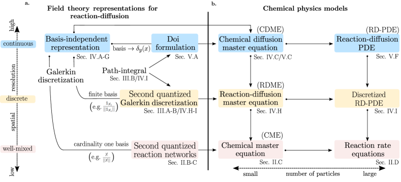
Figure 1: Diagram showing the relations between the main theories and models discussed in this paper along with the section(s) where they are discussed. a. All the field theory representations emerge as special cases of the basis-independent representation of Section IV. These are categorized according to their spatial resolution determined by the basis of the space/subspace used. b. The stochastic chemical physics models corresponding to the field theory representations are shown depending on their spatial resolution. As the number of particles becomes larger, deterministic macroscopic models emerge, which can be obtained employing field theory techniques. Note the basis-independent formulation can be directly used to formulate the CDME and thus other chemical physics models like the discretized RD-PDE in a basis-independent form (Section IV.6). This figure shows the bottom-up relations starting from the basis-independent representation. In the review, we opt for a more instructive approach and present the topic starting from the second quantization of reaction networks.

In this work, we review Fock space and field theoretic methods for stochastic reaction-diffusion systems. We show how the different field theory representations developed historically can all be framed in one unifying basis-independent representation (recently formulated in [179, 182]). We further contextualize how the different field theory representations mirror well-known models of chemical physics depending on their spatial resolution, as well as the corresponding macroscopic (large copy number) limits, which are studied by applied mathematicians, e.g. [5, 191, 135, 177, 116, 115, 225]. The relations between the field theory representations and chemical physics models at different spatial resolution and particle number are all condensed in Fig. 1.

In particular, differing from the original work [179, 182]), we present the basis-independent representation in the bra-ket notation from quantum mechanics [66]. We review well-known approaches, like the Doi formulation and the Doi-Peliti path integral, and we show how these are recovered as special cases of the basis-independent representation. We also illustrate how to perform Galerkin discretizations and how to obtain emergent macroscopic reaction-diffusion partial differential equations (PDEs), as well as how to derive a discretized macroscopic PDE directly from the basis-independent representation. Finally, we formulate alternative representations, such as the flux formulation and the stochastic concentrations, which are essential in establishing connections with tangential fields. It is our aim to present the basis-independent results using a uniform (bra-ket) notation, in a general setting and to highlight connections with existing models.

In what is left of the introduction, we give a more detailed overview and references of previous relevant work, as well as the scope of the theory, various applications and complementary approaches that are not treated in detail in this review. Readers impatient for the formalism can jump directly to Section II.

I.2 Overview of field theories in chemical physics

The simplest model of chemical reactions systems is given by the reaction rate equations formulated by the law of mass action [111, 20, 130, 156]. This consist of a system of deterministic, ordinary differential equations for the evolution of the concentrations in a well-mixed setting. This means that diffusion is assumed to occur at a much faster timescale than reactions; thus the chemical components are distributed uniformly in space, and their spatial distribution does not play a role in the dynamics. It is well-known in the chemical physics community that these differential equations are only valid for large concentrations and that they emerge as large copy-number limit of the underlying stochastic model for well-mixed reaction networks [5]. The stochastic model is called the chemical master equation (CME) [92, 176, 191]. Unlike the rate equations, the state of the system is given by the number of particles and not their concentrations. The CME takes into account the inherent stochastic nature of reactions and describes the time evolution of the probability mass function, which yields the probability of having any given number of particles of each species at any given time. The CME is usually formulated for any chemical reaction network using standard methods; however, one can reformulate it using field-theoretic inspired methods [155, 11, 12]. This yields a second quantized formulation of reaction networks based on classical Fock space representations, illustrated in the bottom right row of Fig. 1. We begin the presentation of these methods in Section II, since it serves as a smooth introduction into the topic.

The concepts of Fock space and second quantization were first introduced in 1932 by the physicist Vladimir Fock in the paper [83] within the scope of many-body quantum mechanics. The problems of many-body quantum mechanics require techniques that are able to deal with indistinguishable entities whose permutations leave the state of the system unchanged. These techniques prepared the ground for quantum field theory [169] and its applications in statistical field theory [2] with the introduction of the so-called creation and annihilation operators, previously introduced in [67]. Such techniques found a natural application in quantum mechanics. A first adaptation of Fock space methods in classical Hamiltonian systems can be found in two consecutive papers [192, 193] by Schönberg, where the second quantization procedure is carried out on the Liouville equation of classical statistical mechanics, and he proposes a way to tackle the mixing paradox proposed by Gibbs by assuming the indistinguishability of classical particles. These techniques have been applied and extended to formulate reaction-diffusion systems in general [68]. For the case of well-mixed reaction networks, where spatial dynamics no longer play a role, the framework is considerably simpler and one can use it to formulate and perform calculations with the CME, often with more ease than with its conventional formulation [11].

In the case of reaction-diffusion processes with full spatial resolution, one needs to keep track not only of the probability of having a certain number of particles of each species, but also their locations. Due to its complexity, the master equation for these processes is not simple to formulate. One can write it in its integro-differential form, but one must handle the combinatorics arising from the indistinguishability and the reactions, while allowing changes in particle numbers. Expanding on the previous work on classical systems by Schönberg (although perhaps unaware of it), the master equation for stochastic reaction-diffusion processes was first constructed in two seminal papers by Masao Doi [68, 69]. He used a field-theoretical representation—now known as the Doi formulation (Fig. 1)—to ease the burden of writing the equation by hand and aid in analytical calculations. The microscopic description is probabilistic, but stochastic in the sense of classical probability theory, not quantum mechanical in the sense of amplitudes. However, we can still employ a Fock space representation to describe the probability distributions governing the systems dynamics [68, 69, 95]. About a decade later, Peliti expanded on this work by discretizing the formulation of Doi into a lattice and constructing a path integral—the Doi-Peliti path integral [167]— with the purpose of calculating observables, estimating perturbations and exploring the renormalization of stochastic reaction-diffusion systems [166]. To facilitate referral to the master equation for reaction-diffusion processes (in analogy to the CME), it has recently been termed the chemical diffusion master equation (CDME) [182, 179], partly due to the term “reaction-diffusion master equation” already being used for the spatially discretized case.

Despite the practical use of previous field theory representations for reaction-diffusion systems (and classical systems), their formulation is hindered by some mathematical difficulties [68, 95]. In contrast with the quantum case, where wave functions live in the space of square integrable functions ($L^{2}$), classical probability densities live in the space of integrable functions ($L^{1}$) (normalized to 1). This compromises the underlying Hilbert space structure of the framework. This issue was formally handled recently [179] by formulating a basis-independent representation of the CDME and by noting which analogies with the original Hilbert space formulation remain valid. This representation recovers previous formulations by employing specific bases, as will be explained in Section IV and illustrated on Fig. 1. This not only justifies previous formalisms from a mathematical perspective but also works as a unifying framework for field theory representations of stochastic reaction-diffusion systems. Although a general methodology to write the CDME in its integro-differential form using standard methods was presented in [182], the field theory representations are advantageous as one can smoothly perform approximations, perturbations, discretizations, calculate equations for first and higher-order moments, and obtain macroscopic models without the need of choosing the underlying basis. Each representation proves to be effectively applicable for a given context, illustrating the power of a unified field theory representation for reaction-diffusion processes.

I.3 Application scope

The applications of stochastic reaction-diffusion systems is remarkably broad, as they form the underlying model for a diverse range of complex systems. Consequently, the field theory representations can find relevant applications in many different fields. One essential application is employing the framework to obtain emergent models at coarser scales. This yields mathematical bridges and relations between parameters of models at different scales that then serve in the development of multiscale numerical schemes. For example, in this work we illustrate this for chemical reaction networks, where one often deals with large numbers of reactants and reaction products. Applying the methodology to a CDME for a bimolecular (nonlinear) reaction systems (see Section V.6), we not only obtain an emergent reaction-diffusion PDE, but also a precise connection between the parameters at the particle level and those of the PDE, enabling consistent multiscale simulation [135, 116]. This kind of methodology can be extended to many other complex systems.

From the computational perspective, it is often convenient to focus on the dynamics in coarser and/or specific regions of phase space. We are thus interested in a formalism that allows us to project the process on a subspace of the whole function space, by means of a Galerkin discretization [131, 171, 195]. This organically leads to the reaction-diffusion master equation (RDME) (see Fig. 1), where the discretization can be on a lattice [114], on metastable regions [224] or others. Simulation schemes and software for such equations have been explored in detail in several works [16, 75, 78, 71, 105, 77]. One advantage of the approach presented here is that the properties of the subspace employed for the Galerkin discretization does not need to be decided a-priori. We can employ the basis-independent formalism to derive emergent macroscopic models, where such subspace can be chosen at the meso- or macroscopic model directly (see Section IV.6). This could then be applied to organically implement adaptive mesh refinement [23, 105] and adaptive moving mesh methods [227] into previously existing methodologies.

Over the years, field theory methods for reaction-diffusion systems have permeated several different fields, ranging from physics to biochemistry, population dynamics and neuroscience. Early work in physics has been mainly focused on the renormalization group analysis [47, 207], computation of critical exponents [120] and the characterization of dynamical phase-transitions [108] in diffusion-controlled chemical reaction networks. Broadly speaking, two types of reactions are considered; the relaxational models [166, 139, 140, 141], where the system eventually reaches an absorbing state, or models with an absorbing state phase transition [120, 94, 49, 51, 123, 121], where there is competition between the absorbing state and particle creation. In both cases, it is possible to use the Doi-Peliti field theory formulation to compute critical exponents in an expansion close to the critical dimension using the renormalization group, as we will review briefly in Section III.4. Other applications in physics concern diffusion-limited reactions [69] and aggregation processes [168, 186, 185], kinetic models such as the (totally) asymmetric exclusion process [189, 7] or kinetically contrained models of glassy dynamics [184, 194, 90, 91, 89, 220], multiple species pair annihilation [62, 107], the contact process [64], sandpile models [221, 222] and applications to exemplary stochastic processes [157, 28].

Field theory methods in the spirit of Doi and Peliti have found further applications in different research fields, marking their use as a general tool for analysing stochastic systems. In cellular and molecular biology, field theories exist for stochastic gene expression [188], stem cell differentiation [229], stochastic gene switching [217], non-equilibrium bacterial dynamics [209], Michaelis–Menten enzyme kinetics [187], RNA dynamics [216], tumor cell migration models [63]. On larger length scales, field theories have been developed to study ecological pattern formation [106, 42, 43], predator-prey dynamics [44] and the spatio-temporal fluctuations in stochastic Lotka-Volterra models [152, 205], swarming and flocking behavior in animals [190, 53] and epidemic spreading models [146, 148, 203]. Another interesting domain of application in recent years is neuroscience, where field theory methods are used to study fluctuations in neural activity [38, 40, 30] and the universal properties of neuronal avalanches [86, 163]. This broad (yet inexhaustive) application domain provides great potential for the basis-independent representation of reaction-diffusion systems to aid in developing multiscale simulations and analysis across many complex systems, constructing bridges between traditionally disparate communities.

I.4 Other relevant and complementary works

Although we cover a large range of topics in this work, there is a large body of work which we do not delve into. Much of this has been presented in detail in the literature and specifically in wonderful reviews. We choose to limit ourselves here to Fock space and field theory methods for master equations describing reaction-diffusion systems (see Fig. 1). Field theory methods have been applied to stochastic differential equations since pioneering work of Feynman-Kac [124], Onsager-Machlup [160] and its formulation due to Martin, Siggia, Rose [144], de Dominicis [70], Janssen [119] and Bausch, Janssen, and Wagner [18]. The connection between all these path integral formulations, together with their connection to forward and backward equations, can be found in the excellent review by Weber and Frey [218].

Other reviews of the Doi-Peliti formalism are by Mattis and Glasser [145], and by Täuber, Howard and Vollmayr-Lee [207], which focuses on the application of renormalization techniques to reaction-diffusion system (see also the book by Täuber [206]). Exactly solvable models are discussed by Schütz [196] and a good field theory review catered to neuroscientists is due to Chow and Buice [54].

Other notable mathematical works have partially investigated similar topics using rigorous measure theory [133]. However, the mathematical complexity often makes it difficult for practitioners to delve into the topic. We also foresee connections between the work we present here and the theory of regularity structures [101], but this requires further research out of the scope of this review.

While there is undoubtedly some overlap with previous works in presenting the Doi-Peliti path integral formalism, this work is meant as a self-contained pedagogical introduction, leading into the less-known basis-independent formulation. We focus mainly on the practical use of the formalism and less on its mathematical rigor. Our main objective is to show how this formulation is related to previous work pertaining to second-quantized stochastic systems and reaction-diffusion models, and to highlight its unifying characteristics and the potential for future applications. This is achieved by developing the quantum-inspired methods and notation at the level of the basis-independent representation, enabling organic connections with previous models. We will further exemplify the robustness of the framework by deriving well-posed numerical discretizations and emerging macroscopic models in a straightforward manner.

I.5 Organization of this paper

The paper is organized as follows: Section II introduces chemical reaction networks in the well-mixed setting, the reaction rate equations and how to formulate the chemical master equation (CME) using Fock space methods, i.e. the second quantized reaction networks formalism. It further shows how to recover the rate equations from the CME using bra-ket notation, as well as how to write generating functions and some remarks related to large deviation theory.

Section III presents the Doi-Peliti path integral formalism of reaction-diffusion systems. We start by introducing discretized spatial dynamics, followed by the derivation of the path integral by taking the continuum limit. We then comment on the perturbative expansion and the renormalization group analysis for reaction-diffusion systems. We close the section with an overview of various application and generalizations of the Doi-Peliti path integral.

Section IV introduces the basis-independent representation, which constitutes a unifying field theory representation for stochastic reaction-diffusion processes. We introduce all Fock space machinery for the generalized case, and we use it formulate the chemical diffusion master equation (CDME) for generic single species chemical reactions, as well as for multiple species nonlinear reactions. We show how to apply a Galerkin discretization to obtain the second quantized Galerkin representation. More specifically, we impose indicator functions as an approximate basis, recovering the starting point from Section III, as well as the so-called reaction-diffusion master equation (RDME) used by chemical physicists. Finally, starting from a generic Galerkin discretization, we present how to write the path integral formalism for the general case. As the discretization is not specified, this results in a basis-independent discretized path integral formulation capable of handling spatially-dependent reaction rates.

Section V discusses limiting cases and alternative representations, specifically in the context of the Doi formulation. First, the original Doi formulation from [68] is recovered as a special limiting case of the basis-independent representation, when Dirac delta functions are used as basis functions, previously demonstrated in [182]. Historically, the spatial discretization of this formulation is the starting point of the Doi-Peliti path integral presented in Section III. Using the Doi formulation, we further write the CDME for a general one species reaction, and we show how to recover the standard representation of the CDME used by physical chemists in terms of scalar probability densities (Fig. 1). We also present how to formulate the master equation in terms of probability fluxes, which is helpful for a thermodynamic analysis. To finalize, we show how to obtain an equation for the dynamics of stochastic concentrations as well as the emergence of macroscopic reaction-diffusion master equations for a nonlinear reaction. This has non-trivial applications to the development of multiscale theory and simulation of complex systems. All these results are obtained employing the bra-ket notation, showcasing the ease with which one can carry different analysis without handling the combinatorics by hand at each stage of the calculation.

II Quantum methods for chemical reaction networks

In this section, we will focus solely on well-mixed chemical reaction networks, where diffusion is assumed to occur at a much faster timescale than reactions. Thus, the chemical components are distributed uniformly in space, and their spatial distribution does not play a role in the dynamics. We will discuss models at two different levels. At the top level, the dynamics of the population (or: densities of chemical compounds) is described by the rate equations; a set of ordinary differential equations describing the change in densities of different species over time. These macroscopic equations are deterministic, continuous and often non-linear. This description emerges as the large copy number limit of a microscopic theory at the bottom level, given by the chemical master equation [5, 88, 92, 176, 191]. This equation models the inherently stochastic reaction processes by quantifying the probabilistic change in discrete particle numbers of each species, due to individual reaction events. This allows one to not only track average quantities, but also study fluctuations from the mean.

We first introduce briefly the rate equations for well-mixed chemical reaction networks, and we formulate the chemical master equation in terms of creation and annihilation operators acting on a Fock space for the number of particles. Then, we show the emergence of the rate equations, followed by a discussion on generating functions, large deviation theory and the application scope. In later sections, we will incorporate space and turn this into a field theory for reaction-diffusion.

II.1 Chemical reaction networks

A chemical reaction network (CRN), loosely speaking, consists out of a set of species $\mathcal{S}$, from which one can form linear combinations (complexes), divided into the reactant $\mathcal{R}$ and the product $\mathcal{P}$ complexes. Additionally, the CRN contains a set of reaction rates labeled by $r\in\mathbb{R}_{\geq 0}$, which can be understood as maps from a reactant complex to a product complex. A more mathematically rigorous definition of a CRN is discussed in [80], however, this is not needed for the current presentation.

Reactions in a CRN are represented with arrows, indicating which reaction complex reacts to form which product complex. For instance, the simple reaction network

$$\mathrm{H}+\mathrm{OH}\to\mathrm{H}_{2}\mathrm{O}\,,$$ (1)

is built from the species $\mathcal{S}=\{\mathrm{H},\mathrm{OH},\mathrm{H_{2}O}\}$, it has complexes $\{\mathrm{H+OH},\mathrm{H_{2}O}\}$ and a single reaction Eq. 1. Another example, now from epidemiology, is the susceptible-infected-susceptible (SIS) model. This simple model of infectious disease spreading supposes the population is divided into people infected by the disease (I) and those susceptible to infection (S). There are two reactions, infection and recovery, which can be represented by a CNR with species $\mathcal{S}=\{\mathrm{S},\mathrm{I}\}$, complexes $\{\mathrm{S+I},2\mathrm{I},\mathrm{I},\mathrm{S}\}$ and two reactions:

$$\mathrm{S}+\mathrm{I} \to 2\mathrm{I}\,,$$ (2a)

$$\mathrm{I} \to\mathrm{S}\,.$$ (2b)

When the expected numbers of particles in the system is very large, random fluctuations in the concentration will be small due to the law of large numbers. The concentrations of each species can then be obtained from the rate equations for the CRN, which follows from the law of mass action. The rate equations for each species $i\in\mathcal{S}$, determine the rate of change $\frac{dx_{i}(t)}{dt}$ for the concentrations $x_{i}(t)$. Each reaction in the network connected to this species will contribute to the rate of change; positively if the species is the reaction product and negatively if it is the reactant. The argument is the same for each reaction, so we can focus on a single reaction first. Let us denote this reaction as:

$$\sum_{i\in\mathcal{S}}m_{i}\mathrm{X}_{i}\to\sum_{i\in\mathcal{S}}n_{i}\mathrm{X}_{i}.$$ (3)

such that $m_{i}$ and $n_{i}$ are the stochiometric coefficients of the species $i$ in the reactant and product complexes, respectively. Let us suppose that this reaction has rate $r$ and involves $s$ species ($|\mathcal{S}|=s$). The law of mass action states that the rate of change of $x_{i}$ due to this reaction is proportional to the concentrations of all reactants, since the reaction only occurs once all of its inputs are present:

$$\frac{dx_{i}}{dt}=r(n_{i}-m_{i})x_{1}^{m_{1}}\ldots x_{s}^{m_{s}}.$$ (4)

Here the reaction vector $(n_{i}-m_{i})$ accounts for the effective number of elements of species $i$ created (or destroyed) in the reaction. The rate equations for our first example (1), are now readily derived as:

$$\frac{dx_{\mathrm{H}}}{dt} =-rx_{\mathrm{H}}x_{\mathrm{O}H}\,,$$ (5a)

$$\frac{dx_{\mathrm{OH}}}{dt} =-rx_{\mathrm{H}}x_{\mathrm{O}H}\,,$$ (5b)

$$\frac{dx_{\mathrm{H_{2}O}}}{dt} =+rx_{\mathrm{H}}x_{\mathrm{O}H}\,.$$ (5c)

The generalization to multiple reactions is straightforward. To reduce the notational complexity, we will first introduce the shorthand notation:

$$\mathbf{x}^{\mathbf{m}}\equiv x_{1}^{m_{1}}\ldots x_{s}^{m_{s}}.$$ (6)

Now each reaction (labelled by $\tau$) has its own rate $r(\tau)\in\mathbb{R}_{\geq 0}$, and consumes $m_{i}(\tau)$ and produces $n_{i}(\tau)$ copies of species $i$. To obtain the rate of change in the expected number of species $i$, one simply sums (4) over all reactions $\tau$

$$\frac{dx_{i}}{dt}=\sum_{\tau}r(\tau)(n_{i}(\tau)-m_{i}(\tau))\mathbf{x}^{\mathbf{m}(\tau)}\,.$$ (7)

For example, for the reaction network (2), if we let $\alpha$ be the infection rate and $\beta$ the recovery rate, we immediately obtain:

$$\frac{dx_{\mathrm{I}}}{dt} =\alpha x_{\mathrm{I}}x_{\mathrm{S}}-\beta x_{\mathrm{I}}\,,$$ (8a)

$$\frac{dx_{\mathrm{S}}}{dt} =-\alpha x_{\mathrm{I}}x_{\mathrm{S}}+\beta x_{\mathrm{I}}\,.$$ (8b)

So, the law of mass action allows one to write down a set of ordinary differential equations (ODEs) corresponding to the reaction network. There are many results relating the dynamics of these ODEs to the geometry of the reaction network, such as the famous deficiency theorems [111, 79], the Anderson-Craciun-Kurtz theorem [4] for the product form of certain CRN equilibrium solutions, or the more recent geometric decomposition into cycles and cocycles proposed in [55]. More information on classical methods to handle the chemical rate equations can be found in the textbooks [20, 130, 156, 225], among others. Here, we will be more interested in connecting the rate equations to a microscopic theory which describes the number of particles of a given species as fluctuating randomly (i.e. stochastically). To do so, we will exploit the similarity with the Fock space representation of quantum mechanics.

II.2 A Fock space for chemical reaction networks

The microscopic description of a chemical reaction network involving $k$ species is given in terms of the probability distribution $p_{\mathbf{n}}(t)$ of having $\mathbf{n}=(n_{1},\dots,n_{s})$ elements of each species, where $n_{i}$ is the copy number for the $i$–th species, at any given time $t$. The dynamics of this probability distribution is given by the chemical master equation (CME) [88, 92, 176, 191], also known in physics as the Kolmogorov-forward equation [132, 82] for the CRN. Although one can formulate the CME using conventional approaches, in this work we will focus on formulating the equation using quantum-inspired methods, which we refer to as the second quantized formulation of reaction networks (Fig. 1), following [68].

Before deriving the equation for $p_{\mathbf{n}}(t)$, we first establish some concepts and notation. We begin by constructing a vector space—the Fock space—for the probability distribution in the copy number representation, using creation and annihilation operators [68, 95, 167]. This essentially exploits the fact that the elements are indistinguishable and their copy number can only change by an integer. We start with defining the empty state $|0\rangle$, the creation operators $a_{i}^{\dagger}$ and annihilation operators $a_{i}$ for the species $i$, such that:

$$a_{i}|0\rangle=0\,,\qquad|\mathbf{n}\rangle=\prod_{i\in\mathcal{S}}(a_{i}^{\dagger})^{n_{i}}|0\rangle\equiv({\mathbf{a}}^{\dagger})^{\mathbf{n}}|0\rangle\,.$$ (9)

Here ${\mathbf{a}}^{\dagger}$ is a vector of creation operators, one for each of the $s$ species in $S$, and $\mathbf{n}\in\mathbb{Z}_{\geq 0}^{s}$ is a vector containing all of their copy numbers. Raising a vector to a vector power is defined as in (6).

The state $|\mathbf{n}\rangle$ represents the system containing $\mathbf{n}=(n_{1},n_{2},\ldots,n_{s})$ copies of the species under consideration. As each one of them is in principle indistinguishable, when we remove (annihilate) a particle of species $i$, there are $n_{i}$ equivalent ways to do so and hence

$$a_{i}|\mathbf{n}\rangle=n_{i}|n_{1},\ldots,n_{i}-1,\ldots,n_{s}\rangle\,.$$ (10)

On the other hand, there is only a single way to add a particle of species $i$, and hence

$$a_{i}^{\dagger}|\mathbf{n}\rangle=|n_{1},\ldots,n_{i}+1,\ldots,n_{s}\rangle\,.$$ (11)

The above relations imply that the creation and annihilation operators satisfy bosonic commutation relations:

$$[a_{i},a_{j}^{\dagger}]=\delta_{ij}\,,\qquad[a_{i},a_{j}]=[a_{i}^{\dagger},a_{j}^{\dagger}]=0\,,$$ (12)

where $[a,b]=ab-ba$ is the commutator. Note that there is nothing quantum mechanical about non-commuting operators; the non-commutativity just means that there is one more way to first add a particle and then remove one, than to first remove a particle and then add one.

An important composite operator is the number operator $N_{i}=a_{i}^{\dagger}a_{i}$, as it counts the number of particles of species $i$ in the state $|\mathbf{n}\rangle$

$$N_{i}|\mathbf{n}\rangle=n_{i}|\mathbf{n}\rangle\,.$$ (13)

Hence, the state $|\mathbf{n}\rangle$ is an eigenvector of the number operators $N_{i}$ with eigenvalues $n_{i}$. We can now define the probability vector $|\rho(t)\rangle$ as:

$$|\rho(t)\rangle=\sum_{\mathbf{n}}p_{\mathbf{n}}(t)|\mathbf{n}\rangle\,,$$ (14)

where $p_{\mathbf{n}}(t)$ is the probability of having $\mathbf{n}$ copies of each species at time $t$. Technically, $|\rho(t)\rangle$ is a vector in the Fock space, defined as the direct sum of symmetric tensor powers of the single particle vector spaces; the states $|\mathbf{n}\rangle$ form a basis for this space.

To compute expectation values (or any other scalar quantity of interest) we also need dual vectors, such that we can take inner products. The full story is a bit more complicated, but for our purpose we can simply define the dual vacuum to be annihilated by the creation operators, and construct a Fock space with annihilation operators:

$$\langle 0|a_{i}^{\dagger}=0\,,\qquad\langle\mathbf{n}|=\langle 0|\prod_{i\in\mathcal{S}}\frac{1}{n_{i}!}a_{i}^{n_{i}}\equiv\frac{1}{\mathbf{n}!}\langle 0|{\mathbf{a}}^{\mathbf{n}}\,.$$ (15)

Additionally, we require $\langle 0|0\rangle=1$. Due to the normalizing factor of $1/\mathbf{n}!\equiv\prod_{i}1/n_{i}!$ in the definition of the dual state, the states $\langle\mathbf{m}|$ and $|\mathbf{n}\rangle$ are orthonormal

$$\langle\mathbf{m}|\mathbf{n}\rangle=\delta_{nm}\,,$$ (16)

and we can write a resolution of the identity as

$$\mathds{1}=\sum_{\mathbf{n}}|\mathbf{n}\rangle\langle\mathbf{n}|.$$ (17)

A special dual state, whose contraction with any vector signifies summing over all components of $|\rho(t)\rangle$, is the flat state denoted as $\langle\mathbf{1}|$. As the probability vector is normalized, we have that:

$$\sum_{\mathbf{n}}p_{\mathbf{n}}(t)=\langle\mathbf{1}|\rho(t)\rangle=1\,.$$ (18)

The flat state signifies summing over all configurations $|\mathbf{n}\rangle$ and hence is given as

$$\langle\mathbf{1}|=\sum_{\mathbf{n}}\langle\mathbf{n}|=\langle 0|e^{\sum_{i\in S}a_{i}}\,.$$ (19)

Here the last equality follows from the definition of the dual state (including the normalization $1/\mathbf{n}!$). It is not hard to verify that the flat state is the left-eigenvector of the creation operators, with eigenvalue $1$

$$\langle\mathbf{1}|a_{i}^{\dagger}=\langle\mathbf{1}|\,,\qquad\forall i\in\mathcal{S}\,.$$ (20)

We are now able to compute expectation values of observables. Any observable $A(\mathbf{n})$ can be cast in terms of creation and annihilation operators $A(a_{i},a_{i}^{\dagger})$. As observables do not modify the system, they do not change the number of particles and are thus expressed with an equal amount of creation and annihilation operators for each species, i.e. they are diagonal operators. The expectation value of $A$ at time $t$ is then computed as

$$\langle A\rangle_{t}=\sum_{\mathbf{n}}A(\mathbf{n})p_{\mathbf{n}}(t)=\langle\mathbf{1}|{A}(a_{i},a_{i}^{\dagger})|\rho(t)\rangle\,.$$ (21)

For example, if we wish to compute the expected value of the number of elements of species $i$, then the observable of interest is the number operator $N_{i}=a_{i}^{\dagger}a_{i}$ and the expectation value becomes

$$\langle N_{i}\rangle=\langle\mathbf{1}|N_{i}|\rho(t)\rangle=\langle\mathbf{1}|a_{i}|\rho(t)\rangle\,.$$ (22)

The last equation here follows from the definition of $N_{i}$ along with equation (20).

The final definitions we need before proceeding to the dynamical equations for $|\rho(t)\rangle$ are the coherent states. These are defined analogously to coherent states in quantum mechanics, although its interpretation is subtly different. A coherent state $|\mathbf{z}\rangle$ is defined in terms of a vector $\mathbf{z}\in\mathbb{R}^{s}$ as

$$|\mathbf{z}\rangle=e^{\sum_{i\in\mathcal{S}}z_{i}a_{i}^{\dagger}}|0\rangle\,.$$ (23)

Here, the exponential of an operator is defined in terms of its infinite power series: $e^{a_{i}^{\dagger}}=\sum_{n}\frac{1}{n!}(a_{i}^{\dagger})^{n}$. The coherent state defines (when properly normalized) a probability distribution over the Fock space, parameterized by the ‘species vector’ $\mathbf{z}$. In fact, it constitutes a multivariate Poisson distribution with the means given by $\mathbf{z}$. In quantum mechanics, coherent states are defined similarly, however there, the vectors $\mathbf{z}$ may be complex and they lead to Poisson distributions with means $|z_{i}|^{2}$.

Similar to the construction above, we can also define dual coherent states as

$$\langle\mathbf{z}|=\langle 0|e^{\sum_{i\in\mathcal{S}}z_{i}a_{i}}\,.$$ (24)

From this definition, we immediately observe that the flat state (19) is a special case of a dual coherent state with all $z_{i}=1$. A useful property of the (dual) coherent states is that they are eigenvectors of the creation and annihilation operators, respectively, with eigenvalue $z_{i}$:

$$\langle\mathbf{z}|a_{i}^{\dagger}=z_{i}\langle\mathbf{z}|\,,\qquad a_{i}|\mathbf{z}\rangle=z_{i}|\mathbf{z}\rangle$$ (25)

II.3 The chemical master equation

Now we are ready to formulate the chemical master equation (CME). This equation describes how the probability of having a certain number of elements of any given species changes in time. Generically, it will have the form

$$\frac{d}{dt}|\rho(t)\rangle=H(a_{i}^{\dagger},a_{i})|\rho(t)\rangle$$ (26)

This equation can be written in standard form [176, 92, 191], so the second quantized bra-ket notation is simply one possible representation. This representation shows great similarity with the (imaginary time) Schrödinger equation, except that here, the ‘Hamiltonian’ ${H}$ is hardly ever Hermitian. In fact, calling $H$ a Hamiltonian may be misleading, since it is in general not Hermitian (as Hamiltonians in quantum mechanics are), nor is it a function specifying the systems energy in equilibrium (as Hamiltonians in equilibrium statistical mechanics are). In the literature $H$ is referred to by many different names, which may depend on the discipline the papers are directed to. We have seen: quasi-Hamiltonian, the infinitesimal generator, the Markov generator, the transition rate matrix, or the time-evolution operator, among others. Here, we will mostly stick to calling $H$ the generator.

The generator should satisfy a number of properties, such that Eq. (26) can describe the time evolution of a probability distribution. First of all, the total amount of probability should be conserved under time evolution. This means that after evolving the system for some time $t$, starting from an arbitrary normalized state $|\rho(0)\rangle$, the state should remain normalized. Since the formal solution of (26) is $|\rho(t)\rangle=\exp(Ht)|\rho(0)\rangle$, this implies that $\langle\mathbf{1}|e^{Ht}|\rho(0)\rangle=1$. But $|\rho(0)\rangle$ is arbitrary, so that

$$\langle\mathbf{1}|e^{Ht}=\langle\mathbf{1}|\,,\quad\forall t\quad\Rightarrow\quad\langle\mathbf{1}|H=0\,.$$ (27)

To put in words, the sum over all states of $H$ should vanish, or: the flat state is a left eigenvector of any generator, with eigenvalue $0$.

Secondly, the generator $H$ should not generate distributions which contain negative probabilities. This implies that any operation implemented by $H$ which changes the number of particles of a certain species should occur with positive sign, otherwise it might be possible to generate negative probabilities. Together with (27), this implies that diagonal terms in $H$ (which do not change the number of particles) should occur with a negative sign, to balance the positive contributions from the reactions which do change the particle numbers.

Lets make this a bit more concrete with an example and then give the general recipe to turn any CRN into a generator $H$. Consider the generic single species reaction displayed in Fig. 2:

$$kA\xrightarrow{\lambda}\ell A$$ (28)

The generator contains a term reflecting the gain in probability of creating $\ell$ particles due to the reaction. A necessary condition for this to occur is that the reaction products are present, so the positive contribution reflecting the change in particle numbers, or the gain, is $\lambda(a^{\dagger})^{\ell}(a)^{k}$, or in words: first annihilate $k$ particles and then create $\ell$ particles.

By itself, this term does not satisfy (27), as $\langle\mathbf{1}|\lambda(a^{\dagger})^{\ell}(a)^{k}\neq 0$. To satisfy the conservation of probability, we should account for the loss of probability of keeping the reactants in the system. This term is negative and diagonal: $-\lambda(a^{\dagger})^{k}(a)^{k}$. The generator of the simple reaction Eq. 28 is then:

$$H=\lambda\left[(a^{\dagger})^{\ell}-(a^{\dagger})^{k}\right](a)^{k}\,,$$ (29)

as displayed in Fig. 2. In a general CRN, for each reaction $\tau$ specified by the transition

$$\sum_{i\in\mathcal{S}}m_{i}(\tau)\mathrm{X}_{i}\xrightarrow{\lambda(\tau)}\sum_{i\in\mathcal{S}}n_{i}(\tau)\mathrm{X}_{i}\,,$$ (30)

we need to add the following terms, corresponding to the gain and loss of probabilities implied by the reaction:

• The term which implements the transition with a positive sign: $\lambda(\tau)({\mathbf{a}}^{\dagger})^{\mathbf{n}(\tau)}{\mathbf{a}}^{\mathbf{m}(\tau)}$

• The negative diagonal term implementing the loss of probability of keeping the reactants: $-\lambda(\tau)({\mathbf{a}}^{\dagger})^{\mathbf{m}(\tau)}{\mathbf{a}}^{\mathbf{m}(\tau)}$.

Hence, to turn any CRN into a generator $H$, we can use the general formula

$$H=\sum_{\tau}\lambda(\tau)\left[({\mathbf{a}}^{\dagger})^{\mathbf{n}(\tau)}-({\mathbf{a}}^{\dagger})^{\mathbf{m}(\tau)}\right]{\mathbf{a}}^{\mathbf{m}(\tau)}$$ (31)

Here we are using the shorthand notation Eq. 6. Note that while the rates $\lambda(\tau)$ of the master equation and $r(\tau)$ of the rate equations are related to each other, they are not equal. The rate $\lambda(\tau)$ specifies the frequency of a single reaction, while the rate $r(\tau)$ specifies the frequency with which the concentrations of elements change.

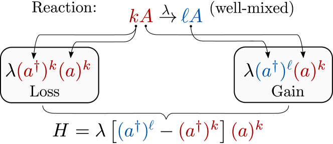
Figure 2: Diagram illustrating how to construct the generator for a system with a general one species reaction with rate $\lambda$ in the well-mixed case.

Any generator $H$ which satisfies the property of conserving non-negative probabilities under time-evolution is called infinitesimal stochastic. These are the stochastic analogues for Hermitian operators in quantum mechanics. However, it is perfectly possible for an operator to be both Hermitian and infinitesimal stochastic. In that special case, the operator will define both a stochastic system (through the master equation) and a quantum system (through the Schrödinger equation) and it is called a Dirichlet operator.

The formal solution of the master equation defines a one-parameter family semigroup of linear operators $U=e^{Ht}$. This operator is a stochastic operator, which map probability vectors into probability vectors. Mathematically, such operators satisfy $\langle\mathbf{1}|{U}(t)=\langle\mathbf{1}|$. We have already encountered stochastic operators in (20); any creation operator $a_{i}^{\dagger}$ is stochastic, since adding one particle does not change the total amount of probability, it merely maps the $n$ particle states to the $n+1$ particle states. This implies that whenever we are computing expectation values of some observables, due to the contraction with $\langle\mathbf{1}|$ from the left, we can set all $a_{i}^{\dagger}\to 1$ after normal ordering.

II.4 Emergence of the rate equations

In this section, we will connect the chemical master equation to the rate equations and see under what assumptions can we go from the microscopic stochastic theory to the macroscopic deterministic theory. This has been done rigorously in mathematical contexts using large copy number limits [5]. Here we want to show how this can be done with techniques using the second-quantized representation.

The macroscopic variables are straightforward to define from the stochastic theory. The concentration of elements of a certain species is simply the expected number of elements of this species, divided by the system volume $V$. So, in accordance with the notation above, we define

$$x_{i}(t)=\langle N_{i}\rangle_{t}=\frac{1}{V}\langle\mathbf{1}|\hat{N}_{i}|\rho(t)\rangle\,.$$ (32)

The next step is to work out the dynamical equations. Using the master equation (26), we can work out what the microscopic theory would give

$$\frac{d}{dt}x_{i}(t)=\frac{1}{V}\langle\mathbf{1}|\hat{N}_{i}H|\rho(t)\rangle=\frac{1}{V}\langle\mathbf{1}|[\hat{N}_{i},H]|\rho(t)\rangle\,.$$ (33)

In the last equality, we have used the property of the generator $\langle\mathbf{1}|H=0$ to express the answer in terms of the commutator. Hence, the time evolution of the expectation value for the number operator (in fact, of any operator) is given by the expectation value of the commutator with the generator $H$; another parallel with quantum mechanics!

For general chemical reaction networks generated by (31), the above relation implies that

$$\frac{d}{dt}x_{i}(t)=\sum_{\tau}\frac{\lambda(\tau)}{V}(n_{i}(\tau)-m_{i}(\tau))\langle\mathbf{1}|\hat{\mathbf{a}}^{\mathbf{m(\tau)}}|\rho(t)\rangle\,.$$ (34)

This is not yet the closed, multi-linear form of the rate equations (7). To bring the right hand side to the desired form, some additional assumptions are needed. Let us focus on a single species for illustrative purposes. Then, the general rate equations (7) are derivable from the master equation when

$$\langle\mathbf{1}|\hat{a}^{m}|\rho(t)\rangle-\langle\mathbf{1}|\hat{a}|\rho(t)\rangle^{m}=0\,.$$ (35)

If this equation holds, we may replace $\langle\mathbf{1}|\hat{a}|\rho(t)\rangle$ by $Vx(t)$ and we get

$$\frac{dx_{i}(t)}{dt}=\sum_{\tau}\lambda(\tau)V^{\sum_{i}m_{i}(\tau)-1}(n_{i}(\tau)-m_{i}(\tau))\mathbf{x}^{\mathbf{m}(\tau)}$$ (36)

This is exactly equal to the rate equation if we identify $r(\tau)=V^{\sum_{i}m_{i}(\tau)-1}\lambda(\tau)$.

Equation (35) constitutes a mean-field approximation; it supposes that the $m$-th moment of the number operator is given by the $m$-th power of the expectation value. This is a simplification of the process, which is a good first approximation, but of course, it is not exactly true when variances are large. However, when the total number of elements is big, the law of large numbers and the central limit theorem offer a helping hand. The law of large numbers roughly states that for $n$ independent and identically distributed (iid) random variables $\{X_{n}\}$, the sample mean $S_{n}=\frac{1}{n}\sum_{n}X_{n}$ will converge to the mean $\mu$ of the distribution from which the $X_{n}$ are sampled, namely $\lim_{n\to\infty}S_{n}=\mu$. The central limit theorem states that in the same large $n$ limit, the distribution of the sample mean $S_{n}$ becomes Gaussian with standard deviation $\sigma/\sqrt{n}$, where $\sigma$ is the standard deviation of the distribution for the random variables. Or

$$S_{n}\to\mu+\xi/\sqrt{n}\,,$$ (37)

where $\xi$ is normally distributed $\mathcal{N}(0,\sigma^{2})$. This in particular implies that the expectation value of any power of the sample mean $S_{n}^{k}$ will tend to the power of the mean $\mu^{k}$, with subleading corrections proportional to $\frac{1}{n}$. These corrections vanish in the large $n$ limit.

In our case, we can apply this when we assume that the number of elements of each species is very large, or likewise, if we are considering the dynamics of concentrations of species in a large volume expansion of the CRN. In chemistry this is called the van Kampen expansion, after [212]. In these situations, and assuming the elements are iid, we can approximate $\langle a^{k}\rangle$ as $\langle a\rangle^{k}$ and in this limit we recover the rate equations (7) from the master equation of the system. In other words, the leading contributions in a large $V$ expansion of (34) gives the rate equation (36), and the corrections to this equation vanish as $1/V$ in the limit $V\to\infty$.

II.5 Generating functions

The probability vector $|\rho(t)\rangle$ gives us a formal way of representing an infinite sequence of numbers, representing the probability of the system to have a certain copy number $\mathbf{n}$. In mathematics, and specifically in probability theory, another useful representation of infinite sequences is through a generating function. The generating function encodes an infinite sequence of numbers ($a_{n}$) by treating them as coefficients of a formal power series of a variable $z$. If the infinite sequence $a_{n}$ has a finite sum, then the formal power series will converge and if we are lucky we may even obtain a closed form expression for the generating function in terms of analytic functions of the variable $z$. In general, we will see that it is possible to derive a partial differential equation for the probability generating function of a generic CRN. Afterwards, we will define the moment generating function of an observable, where the series coefficients $a_{n}$ are not the probabilities $p_{\mathbf{n}}(t)$, but the different statistical moments of an observable: $\langle\hat{O}^{n}\rangle$.

Formally, the generating function for an infinite series $a_{n}$ is defined as

$$G(a_{n};z)=\sum_{n}a_{n}z^{n}\,.$$ (38)

This naturally generalizes to multiple variables. If we suppose there are $s$ species, then

$$G(a_{\mathbf{n}};\mathbf{z})=\sum_{\mathbf{n}}a_{\mathbf{n}}\mathbf{z}^{\mathbf{n}}\,.$$ (39)

Here we make use of the notation introduced in (6). The generating function is now a formal power series in $s$ variables, where $s$ is the number of different species $s=|\mathcal{S}|$. To obtain the probability generating function from the probability vector $|\rho(t)\rangle$, we can make use of the dual coherent state $\langle\mathbf{z}|$ defined in Eq. 24, together with its eigenvalue equation Eq. 25

$$G(\mathbf{z},t)=\langle\mathbf{z}|\rho(t)\rangle=\sum_{\mathbf{n}}p_{\mathbf{n}}(t)\mathbf{z}^{\mathbf{n}}\ .$$ (40)

The probability generating function has a number of useful and interesting properties. Lets go through a few in the case of a single species to lighten up the notation. The generalization to multiple species is immediate. First, the normalization of $|\rho(t)\rangle$ is now translated to the property that the probability generating function evaluated at $z=1$ equals $1$

$$G(z=1,t)=\langle 1|\rho(t)\rangle=1$$ (41)

Then, if we wish to recover the probability mass function $p_{n}(t)$ giving the probability of having $n$ elements, we can do so by taking $n$ derivatives with respect to $z$, followed by evaluating the result at $z=0$

$$p_{n}(t)=\left.\frac{1}{n!}\frac{d^{n}G(z,t)}{dz^{n}}\right|_{z=0}$$ (42)

The expectation value for the number of elements at time $t$ is also extracted by taking derivatives, but now evaluated at $z=1$

$$\langle N\rangle_{t}=\left.\frac{d}{dz}G(z,t)\right|_{z=1}\,.$$ (43)

If we wish to compute higher moments of the number operator, we can do so by the following relation

$$\langle N^{n}\rangle_{t}=\left.\left(z\frac{d}{dz}\right)^{n}G(z,t)\right|_{z=1}\,.$$ (44)

It should be understood here that one first performs the operation $\left(z\frac{d}{dz}\right)^{k}$ on the generating function and only afterwards set $z=1$. This expression invites the identification of the number operator $N=\hat{a}^{\dagger}\hat{a}$ with $z\frac{d}{dz}$, such that creation operators correspond to multiplications with $z$ and annihilation operators are differentiation with respect to $z$. Indeed, speaking in terms of probability generating functions is completely equivalent to making the following identifications in the formalism developed in the last sections

$$a_{i}^{\dagger}\to z_{i}\,,\qquad a_{i}\to\frac{\partial}{\partial z_{i}}\,.$$ (45)

As for example presented in [11], this representation of the creation and annihilation operators satisfies the canonical commutation relations (12) and allows us to write the general master equation in terms of a partial differential equation for the probability generating function

$$\partial_{t}G(\mathbf{z},t)=\sum_{\tau}\lambda(\tau)(\mathbf{z}^{\mathbf{n}(\tau)}-\mathbf{z}^{\mathbf{m}(\tau)})\partial_{\mathbf{z}}^{\mathbf{m}(\tau)}G(\mathbf{z},t)\,.$$ (46)

Here, we are still using the shorthand notation for exponentials (6) and $\partial_{\mathbf{z}}^{\mathbf{m}}=\prod_{i\in\mathcal{S}}\left(\frac{\partial}{\partial z_{i}}\right)^{m_{i}}$. Here are two simple examples which illustrate the computation of the probability generating function

The Poisson process $\emptyset\to A$.

The equation for the probability generating function is

$$\partial_{t}G(z,t)=\lambda(z-1)G(z,t)\,.$$ (47)

Together with the initial condition of having zero elements at $t=0$, which translates to $G(z,0)=1$, this is easily solved as $G(z,t)=e^{\lambda t(z-1)}$, which is indeed the well-known result for the generating function of the Poisson process.

The pure death process $A\to\emptyset$.

The differential equation for $G(z,t)$ is now

$$\partial_{t}G(z,t)=\lambda(1-z)\partial_{z}G(z,t)\,.$$ (48)

A trick to solve these kinds of equations is to find a characteristic curve $c$ in terms of $z$ and $t$, such that $G(z,t)=f(c(z,t))$. We can do this by supposing that $z$ has some implicit time dependence, such that $G$ is a function of $z(t)$ and $t$ and the equation (48) splits into two equations

$$\frac{d}{dt}G(z(t),t)=0\,,\qquad\frac{d}{dt}z(t)=\lambda(z-1)\,.$$ (49)

The latter equation is solved by $z(t)=1+ce^{\lambda t}$, which introduces a constant $c$. Solving for $c$ gives

$$c=(z-1)e^{-\lambda t}\,,\quad\text{such that: }\,\,G(z,t)=f(c(z,t))\,.$$ (50)

One can verify readily that $f(c)$ obeys equation (48) when $c$ is given as above. The final step is to consider the initial conditions. If at $t=0$, there are $k$ particles present, then we must have $G(z,0)=z^{k}$ and this then fixes the functional form of $f(c)$ to be $(1+c(z,0))^{k}$ such that

$$G(z,t)=(1+e^{-\lambda t}(z-1))^{k}\,.$$ (51)

Although it is generally a rare treat to find exact solutions for more involved CRNs, there are some noticeable examples in the literature (see [118] for a classical approach to solving monomolecular CRNs). In [99], exact solutions of the generating function PDE for a stochastic model of a gene regulatory feedback loop are presented. See [215, 216] for exact solutions of monomolecular and stochastic gene switching reaction networks in a second quantized formulation.

II.5.1 Moment generating functions

The moment generating function for the observable $\hat{O}$ is defined as the generating function for the series $a_{n}=\langle\hat{O}^{n}\rangle/n!$. This is equivalent to the expectation value of $e^{z\,\hat{O}}$, where $z$ is the variable of the power series. In the second quantized framework

$$M_{\hat{O}}(z,t)=\langle e^{z\,\hat{O}}\rangle_{t}=\langle\mathbf{1}|e^{z\,\hat{O}}|\rho(t)\rangle\,.$$ (52)

For instance, if the observable is the number operator for species $i$, then we can express its moment generating function as

$$M_{\hat{N}_{i}}(z_{i},t)=\langle\mathbf{1}|e^{z_{i}\hat{N}_{i}}|\rho(t)\rangle$$ (53)

We can also construct the moment generating function for number operators of all species, which will then depend on a vector of variables $\mathbf{z}$

$$M_{\hat{\mathbf{N}}}(\mathbf{z},t)=\langle\mathbf{1}|e^{\mathbf{z}\cdot\hat{\mathbf{N}}}|\rho(t)\rangle\,,$$ (54)

where $\mathbf{z}\cdot\hat{\mathbf{N}}=\sum_{i\in\mathcal{S}}z_{i}\hat{N}_{i}$. If we now use the fact that $|\rho(t)\rangle=e^{Ht}|\rho(0)\rangle$ and (31) for the generic generator of a chemical reaction network, then, by commuting the $\hat{N}_{i}$’s though $H$ using (12), we may write

$$M_{\hat{\mathbf{N}}}(\mathbf{z},t) =\langle\mathbf{1}|e^{\mathbf{z}\cdot\hat{\mathbf{N}}}e^{Ht}|\rho(0)\rangle$$ (55)

$$=\langle\mathbf{1}|e^{\tilde{H}(\mathbf{z})t}e^{\mathbf{s}\cdot\hat{\mathbf{N}}}|\rho(0)\rangle\,,$$ (56)

with

$$\tilde{H}(\mathbf{z})=\sum_{\tau}\lambda(\tau)\left[e^{\mathbf{z}\cdot(\mathbf{n}(\tau)-\mathbf{m}(\tau))}(\hat{\mathbf{a}}^{\dagger})^{\mathbf{n}(\tau)}-(\hat{\mathbf{a}}^{\dagger})^{\mathbf{m}(\tau)}\right]\hat{\mathbf{a}}^{\mathbf{m}(\tau)}\,.$$ (57)

The moment generating function is related to the exponential of a so-called tilted generator $\tilde{H}(\mathbf{z})$ (sometimes also called deformed or biased generator), which is easily obtained from the Markov generator $H$ by replacing the creation operators and annihilation operators as:

$$a_{i}^{\dagger}\to e^{z_{i}}a_{i}^{\dagger}\,,\qquad a_{i}\to e^{-z_{i}}a_{i}\,.$$ (58)

This procedure allows one to immediately write down the moment generating function of the number operators as the exponential of the tilted generator. For example, for the Poisson process $\emptyset\to A$, the tilted generator is $\tilde{H}(z)=\alpha(e^{z}\hat{a}^{\dagger}-1)$. When starting with zero elements, we have $e^{z\hat{N}}|\rho(0)\rangle=|0\rangle$, such that we immediately obtain the moment generating function

$$M_{\hat{N}}(z,t)=\langle\mathbf{1}|e^{\alpha t(e^{z}\hat{a}^{\dagger}-1)}|0\rangle=e^{\alpha t(e^{z}-1)}\,.$$ (59)

This is the well-known expression for the moment generating function of the Poisson point process with mean $\alpha t$.

II.6 The large deviation principle

We saw in the last section how the moment generating function for the number operator is given by the exponential of a tilted generator. A similar tilted generator can also be defined for another observable, called the dynamical activity $K$. This observable is not easily expressible in terms of creation and annihilation operators, because it is a trajectory dependent observable. The dynamical activity counts the total number of reactions which have taken place at a given time $t$. Since the reactions occur by a random process, the dynamical activity $K$ is a random variable.

To obtain the moment generating function $M_{K}(s,t)$ for the dynamical activity $K$, following [90, 91], we have to adapt our formalism slightly. We not only track the probabilities $|\rho(t)\rangle$, but we define the vector $|\rho(t,k)\rangle$, which gives the probability of having a certain combination of copy numbers at time $t$ and having seen $k$ reactions since $t=0$. Then, the moment generating function for the dynamical activity becomes

$$M_{K}(z,t)=\langle e^{zK}\rangle_{t}=\sum_{k=0}^{\infty}\langle\mathbf{1}|e^{zk}|\rho(t,k)\rangle=\langle\mathbf{1}|\tilde{\rho}(t,z)\rangle$$ (60)

Here we have defined the tilted probability vector $|\tilde{\rho}(t,z)\rangle=\sum_{k}e^{zk}|\rho(t,k)\rangle$ as the (discrete) Laplace transform of $|\rho(t,k)\rangle$. It is possible to show that for a general chemical reaction network, the tilted probability vector obeys the following (tilted) master equation

$$\partial_{t}|\tilde{\rho}(t,z)\rangle=\tilde{H}(z)|\tilde{\rho}(t,z)\rangle\,,$$ (61)

with

$$\tilde{H}(z)=\sum_{\tau}\lambda(\tau)\left[e^{z}(\hat{\mathbf{a}}^{\dagger})^{\mathbf{n}(\tau)}-(\hat{\mathbf{a}}^{\dagger})^{\mathbf{m}(\tau)}\right]\hat{\mathbf{a}}^{\mathbf{m}(\tau)}\,.$$ (62)

So the tilted generator for the dynamical activity is obtained by multiplying the gain terms (which generate reactions) with $e^{z}$. The formal solution to (61) is now $|\tilde{\rho}(t,z)\rangle=e^{\tilde{H}(z)t}|\rho(0)\rangle$, assuming that there has been no activity initially, so $K=0$ at $t=0$. This implies that the moment generating function is the exponential of the tilted generator:

$$M_{K}(z,t)=\langle\mathbf{1}|e^{\tilde{H}(z)t}|\rho(0)\rangle\,.$$ (63)

We can think of this quantity, (or any moment generating function for that matter) as the analogue to a partition function in equilibrium statistical mechanics. Only here the observable is not energy with dual parameter inverse temperature ($\beta$), but it is the tilted generator, for which time serves as dual parameter. The interpretation is that this encapsulates information on the dynamical activity $K$ (which has dual parameter $z$) at any time.

A modern approach to statistical mechanics is given in a subject called large deviation theory. We will not give an exhaustive review of this, but rather refer to the review of Hugo Touchette [210] for a historical and topical background on this fascinating subject, which connects statistical mechanics with the mathematics of probability theory and the analysis of rare events. A review on large deviation theory in the context of the non-equilibrium dynamics of stochastic reaction-diffusion systems is provided in [201].

In the context of this section, we are interested in how the dynamical activity will behave at late times, so in the limit of $t\to\infty$. The large deviation principle states that the probability of seeing events with activity $k$ decays exponentially according to

$$P(k,t)\propto\exp(-tI(k/t))\,.$$ (64)

Here $I(k)$ is the rate function (also called the Cramér function, or the entropy rate function). The rate function has the property that its zeros define the expected values of $k/t$, as for these values the probability $P(k,t)$ does not decay in time. For all other values of $k/t$, the rate function determines the late time decay rate of the probability of seeing these events, and hence it contains information on how probabilities for observing events deviating from the mean behave.

The rate function is related to the moment generating function in the following way. It is the Legendre-Fenchel transform of the scaled cumulant generating function (SCGF) $\Theta(z)$, or

$$I(k)=\sup_{z}(k\,z-\Theta(z))\,,$$ (65)

where $\Theta(z)$ is defined as

$$\Theta(z)=\lim_{t\to\infty}\frac{1}{t}\log M_{K}(z,t)\,.$$ (66)

This definition is equivalent to stating that the moment generating function $M_{K}(z,t)$ behaves as

$$M_{K}(z,t)\propto e^{t\Theta(z)}\,,$$ (67)

when $t\to\infty$. As we have just seen, the moment generating function is the exponential of the tilted generator (62), and hence the leading contribution to $M_{K}(z,t)$ will come from the largest eigenvalue of $\tilde{H}(z)$. This argument relates the SCGF to the leading eigenvalue of the tilted generator as a function of $z$. Hence, to find the large deviation rate function, we need to compute the Legendre-Fenchel transform of the SCGF $\Theta(z)$, which can be found by optimizing for the leading eigenvalue of the tilted generator; similar to performing a ground state optimization in many-body quantum systems. Only in this case, the Hamiltonian is a tilted generator, which in general is not Hermitian, and neither is it infinitesimal stochastic, since the exponential tilting spoils this property. Hence, its computation is generically not simple and might involve extensive numerical computations.

The large deviation principle is not always guaranteed to exist, just as the leading eigenvectors of $\tilde{H}(z)$ are not always unique. In some cases, the eigenvalue decomposition of $\tilde{H}(z)$ does not exist (as not all matrices are diagonalizable). Generally, a CRN (or Markov process in general) with absorbing states are going to cause problems, since the dynamics can get stuck in absorbing states, which makes the late time properties sensitive to the initial conditions. However, for systems which are ergodic, such that every microscopic configuration can be reached from any other configuration by a series of transitions, the leading eigenvalue of $\tilde{H}$ is unique and these methods are very powerful.

For further reading on the relationship between large deviation theory and chemical reaction networks we refer to the reviews [201, 10], which also use field theory methods similar to the theory presented here. A sample path Large Deviation Principle for a large class of CRNs was discussed in [3]. Dynamical Large Deviations in the large volume limit are discussed in [138], where it is shown that CRNs with multiple steady states generically undergo a first-order dynamical phase transitions in the vicinity of zero tilting parameter.

II.7 Applications and further advances

The Fock space approach to chemical reaction networks and stochastic dynamics has found applications in a diverse range of disciplines. Here we list a selection of references which make use of these methods in the setting where populations are considered to be stochastic, but homogeneously mixed (well-mixed). Models with (discrete or continuous) spatial degrees of freedom are discussed in the following sections.

An application to the Malthus-Verhulst process which essentially represents logistic growth, are discussed in [153]. Other results in population dynamics are found in [187], which provides exact solutions of stochastic Michelson-Mentis enzyme kinetics, and [203] treats stochastic finite-size SIR epidemic models. Analytical solutions of biological models of gene transcription involving bursting and gene switching are described in [216]. An application of these methods to stochastic game theory on a population level was discussed in [9], where a risk averse utility measure based on the moment generating function was shown to lead to cooperative behaviour in population games. Further applications in an economic setting were made in [27, 26], where stochastic models of limit order books are described by creation and annihilation operators of orders. In physics these methods were used to uncover the statistics of electron-hole avalanches in semiconductors exposed to an electric field [223] and to describe neutron population under the influence of a feedback mechanism in nuclear reactors as a stochastic field theory in [59]. Models of stochastic graph-rewriting leveraging a Fock space description were presented in [21].

The second quantized approach to stochastic mechanics has also been used to further our theoretical understanding of chemical master equations and their properties. A one-parameter family of extensions of the second quantized stochastic mechanics is related to orthogonal Hermite and Charlier polynomials [159]. In [13] a Noether theorem for stochastic systems was derived using Fock space methods and an alternate proof of the Anderson-Craciun-Kurtz (ACK) theorem was presented in [14]. A generalization of the ACK theorem to a class of CRNs without zero deficiency or weak reversibility was presented in [109], making use of squeezed coherent states in Fock space. The link between dynamical equations for the probability generating functions, the exponential moment generating functions, the factorial moment generating functions and results in mathematical combinatorics was made more explicit in [22]. Equations of motion for the moments of the density operator at all orders for stochastic CRNs at general deficiency were derived in [202]. The connection between the second quantized formalism for ecosystem dynamics and mean-field biochemical reaction networks was discussed in [58]. Work on an action functional gradient descent algorithm for finding escape paths (i.e. least improbable or first passage paths) in stochastic CRN with multiple fixed points is presented in [84].

III Incorporating space: field theories for reaction-diffusion

In the last section we described the dynamics of CRNs at two levels: the rate equations for the deterministic dynamics of concentrations and the chemical master equation for the stochastic dynamics of copy numbers. In both modeling approaches, the well-mixed assumption results in the lack of spatial dependence, making the description valid only when spatial factors do not play a significant role in the system dynamics.

The purpose of this section is to relax the well-mixed assumption and introduce spatial dependence into the microscopic probabilistic model from the previous section. To do so, we discretize diffusion as reactions that add or remove particles in given voxels in space, which enable us to apply the mathematical methods from the last section. The limit of decreasing voxel size will lead to a continuous statistical field theory for reaction-diffusion systems. Now, instead of having a finite and constant probability of reacting with one-another, particles rely on diffusion to be brought into the vicinity of one another. These are also called diffusion-influenced reactions. In chemistry, it means the solution should not be stirred, but the reactants are depending on Brownian motion to be brought within interaction range. In population biology, we may think of members of a species performing a random walk through an environment in order to find each other.

We will first briefly review the relation between random walks and the diffusion equation and formulate this in terms of the second-quantized description of the last section. Then, following [93, 167] we will turn the master equations for the reaction systems of the last section into a field theory for non-equilibrium reaction-diffusion systems. We derive the propagator of the free theory for reaction-diffusion systems and note that this is nothing else than the Green’s function for the diffusion equation. Finally, we briefly comment on the perturbative expansion and renormalization group methods for reaction-diffusion systems. The aim is to give a pedagogical introduction to the construction of a reaction-diffusion path integral (also known as the Doi-Peliti path integral). For a deeper dive into this subject, we refer to the reviews [207, 54], the book [206] and [46, 51].

III.1 Random walks and the emergence of diffusion

The microscopic diffusion process can be modeled as a random walk on a regular lattice by means of a master equation. More details on this exemplary subject which lies at the heart of many processes in non-equilibrium statistical physics can be found in [113, 136]. Here, we will focus on introducing the Fock space description of the random walk and its continuous limit to the diffusion equation. To this end, we need a regular, $d$-dimensional lattice with lattice spacing $h$ and suppose that a particle has equal probability of hopping to any neighboring site. Importantly, each walker’s hopping probability is independent of the presence of any other walker or of its own past trajectory. This means that we can treat the walkers as independent and identically distributed (iid) and that the random walk allows for a Markovian description.

Let us first consider random walkers of a single species $A$. The probability vector $|\rho(t)\rangle$ will now be expanded into a Fock space for the lattice occupation numbers $\{n\}$, representing the number of walkers $n_{i}$ per lattice site $i$, such that: $|\rho(t)\rangle=\sum_{\{n\}}p_{\{n\}}(t)\prod_{i}(a^{\dagger}_{i})^{n_{i}}|0\rangle$. Hence, now we suppose that $a_{i}$, and $a^{\dagger}_{i}$ are the annihilation and creation operators for species $A$, but at lattice site $i$. The random walk master equation is then:

$$\partial_{t}|\rho(t)\rangle =\frac{D}{h^{2}}\sum_{(i\,j)}\big{[}a^{\dagger}_{j}a_{i}-a_{i}^{\dagger}a_{i}+a_{i}^{\dagger}a_{j}-a^{\dagger}_{j}a_{j}\big{]}|\rho(t)\rangle$$

$$=-\frac{D}{h^{2}}\sum_{(i\,j)}\big{(}a_{i}^{\dagger}-a^{\dagger}_{j})(a_{i}-a_{j})|\rho(t)\rangle$$

$$\equiv H_{0}(D)|\rho(0)\rangle\,.$$ (68)

Here $(i\,j)$ is shorthand notation for nearest neighbours. The hopping rate is set (with some amount of hindsight) to $\frac{D}{h^{2}}$, where $D$ will become the diffusion constant in the continuous $h\to 0$ limit. Let us take this continuous limit for the observable counting the local density of particles at site $i$, defined as:

$$\rho_{i}(t)=\frac{1}{V}\langle\hat{N}_{i}\rangle_{t}=\frac{1}{V}\langle\mathbf{1}|a_{i}|\rho(t)\rangle$$ (69)

From (33), together with (68), it is not hard to work out that for the one-dimensional lattice:

$$\partial_{t}\rho_{i}(t)=\frac{D}{h^{2}}\left[\rho_{i+1}(t)+\rho_{i-1}(t)-2\rho_{i}(t)\right]$$ (70)

where $\rho_{i\pm 1}(t)$ denotes the local density at the neighboring lattice sites. Taking the limit $h\to 0$, we replace $\rho_{i}(t)\to\rho(x,t)$, such that $\rho_{i\pm 1}(t)\to\rho(x\pm h,t)$. After Taylor expanding $\rho(x,t)$ around $x$, this gives the one-dimensional diffusion equation

$$\partial_{t}\rho(x,t)=D\partial_{x}^{2}\rho(x,t)\,.$$ (71)

Generalization of the above argument to a $d$-dimensional lattice results in the $d$ dimensional diffusion equation

$$\partial_{t}\rho(\mathbf{x},t)=D\nabla^{2}\rho(\mathbf{x},t)\,,$$ (72)

where $\nabla^{2}=\vec{\nabla}\cdot\vec{\nabla}$ is the Laplacian. The solution to this equation for a normalized density with an initial distribution localized at $x=0$ can be found by Fourier transformation and reads:

$$\rho(\mathbf{x},t)=\frac{1}{(4\pi Dt)^{d/2}}e^{-\frac{x^{2}}{4Dt}}\,.$$ (73)

So we see that the density behaves as a (multivariate) normal distribution with vanishing mean and variance growing linearly in time as $2Dt$. This implies that, while the expected position of the walker does not change in time, its mean squared displacement grows linearly in time, allowing the walker to explore a sphere around the origin of radius $\sqrt{Dt}$. Note that the density satisfying (72) does not have to be normalized (it is in general a concentration), and may satisfy other boundary conditions or initial conditions as those leading to (73). For example, constant Dirichlet boundaries imply contact with an external reservoir [180, 135].

The generalization to multiple species is immediate, although notationally more cumbersome. Now there is a set of occupation numbers for each species $s\in\mathcal{S}$. Let us denote the total set of $|\mathcal{S}|$ occupation numbers $\{n\}_{\mathcal{S}}$. Then $|\rho(t)\rangle$ is expanded in the basis

$$|\{n\}_{\mathcal{S}}\rangle=\prod_{i}\prod_{s\in\mathcal{S}}(a_{i,s}^{\dagger})^{n_{i,s}}|0\rangle\,.$$ (74)

where here $a_{i,s}^{\dagger}$ is the creation operator for species $s$ at lattice site $i$ and $n_{i,s}$ is the number of particles of species $s$ at lattice site $i$. Fortunately, the random walk process for each species is independent of any other species, and so the multi-species diffusion generator $H_{0}(\{D\}_{\mathcal{S}})$ is just the sum of the single species diffusion generators, where each species $s$ may have a different and independent diffusion constant $D_{s}$

$$H_{0}(\{D\}_{\mathcal{S}})=\sum_{s\in\mathcal{S}}H_{0}(D_{s})\,.$$ (75)

In applications, one could have other forms of diffusion such as non-Laplacian diffusion or interacting diffusion through pair potential interactions [65]. Asymmetric diffusion, where particles have a preference for diffusing in a certain direction, is treated in [189]. Related to this is the asymmetric exclusion process, which combines asymmetric diffusion with a particle exclusion principle at each site [142, 196]. In [8] a Fock space formalism for Lévy flights was introduced, which agrees with Lévy distributions in the continuous limit. When the underlying geometry is not a regular lattice, but rather complex network, the diffusion generator (68) becomes the graph Laplacian; the generator for random walks on a graph [41]. More involved stochastic models on complex networks, such as spreading models, can also be formulated in using an operator formalism, as was done in [146, 147]. Here, however, we will focus on the continuous limit, leading to a field theory formulation.

III.2 The Doi-Peliti path integral for reaction-diffusion systems

In this section, we will outline the continuum limit of the second-quantized representation of stochastic mechanics, leading to a field theory for reaction-diffusion systems, first discussed in this context for the birth-death processes ($A\to 2A$ and $A\to\emptyset$) by Peliti in [167]. Hence this framework is sometimes called the Peliti path integral representation—or the “Doi-Peliti” path integral, since it builds on the theory by [68]. The construction here supposes that particles become point-particles in the continuum limit and reactions only take place when reactants are found at the same location in space. This has issues from a mathematical perspective: two point particles would encounter each other at exactly the same location in space with probability zero. However, this is a common physical approximation as one usually ends up working with discretizations and/or densities instead of individual particles. In LABEL:{sec:stochMecRD}, we will discuss a more general stochastic field theory which is basis-independent and can handle arbitrary, space dependent rate functions. The theory by [68] is recovered as a limiting case in Section V.1, as depicted in Fig. 1, which in turn verifies the Peliti path integral representation presented here.

As before, we restrict the presentation to a single species general reaction $kA\to\ell A$. The generalization to multiple species is not difficult and follows analogously. The reaction-diffusion generator $H$ consists of the diffusion generator $H_{0}(D)$ (68) and the reaction generator $H_{I}$, given in (31). We further assume that only particles at the same lattice location can react. This implies that:

$$H =H_{0}(D)+H_{I}(\{\lambda\})\,,$$

$$=-\frac{D}{h^{2}}\sum_{(i\,j)}\big{(}a_{i}^{\dagger}-\hat{a}^{\dagger}_{j})(a_{i}-\hat{a}_{j})$$

$$\qquad+\sum_{i,\tau}\lambda(\tau)\left[(a_{i}^{\dagger})^{\ell(\tau)}-(a_{i}^{\dagger})^{k(\tau)}\right]a_{i}^{k(\tau)}\,.$$ (76)

Somewhat suggestively, we have already named the diffusive part of the generator $H_{0}$ and the reactive part $H_{I}$, foreshadowing the fact that in the final action we can treat $H_{0}$ non-perturbatively, as the ‘free theory’ for reaction-diffusion systems, but we should treat the final action perturbatively with respect to the non-linearities induced by the reactions in $H_{I}$.

To proceed, it is convenient to introduce coherent states defined in terms of a complex valued variable $\eta$ as:

$$|\eta\rangle=e^{-\frac{1}{2}|\eta|^{2}}e^{\eta\hat{a}^{\dagger}}|0\rangle\,,\quad\langle\eta|=\langle 0|e^{\eta^{*}\hat{a}}e^{-\frac{1}{2}|\eta|^{2}}\,.$$ (77)

Here the star denotes complex conjugation. The overlap between two of these states can be shown to give:

$$\langle\eta_{1}|\eta_{2}\rangle=e^{-\eta_{1}^{*}(\eta_{1}-\eta_{2})}e^{\frac{1}{2}|\eta_{1}|^{2}-\frac{1}{2}|\eta_{2}|^{2}}\,.$$ (78)

The complex valued coherent states define a resolution of the identity operator as:

$$\mathds{1}=\int\frac{\mathrm{d}^{2}\eta}{\pi}|\eta\rangle\langle\eta|\,,$$ (79)

or, defining one coherent state for each lattice site $i$:

$$\mathds{1}=\int\prod_{i}\left(\frac{\mathrm{d}^{2}\eta_{i}}{\pi}\right)|\bm{\eta}\rangle\langle\bm{\eta}|\,,$$ (80)

where $\mathrm{d}^{2}\eta_{i}=\mathrm{d}\mathrm{Re}(\eta_{i})\mathrm{d}\mathrm{Im}(\eta_{i})$ and $|\bm{\eta}\rangle=|\eta_{1}\rangle\otimes|\eta_{2}\rangle\otimes\ldots$.

We now proceed to define the path-integral for the expectation value of any observable $\hat{A}$. First, we write the expectation value in terms of the formal solution of the master equation as $\langle A\rangle_{t_{f}}=\langle\mathbf{1}|\hat{A}e^{Ht_{f}}|\rho(0)\rangle$. Then, the time evolution induced by the generator $H$ is divided into infinitely many slices of infinitesimal size

$$e^{Ht_{f}}=\lim_{\Delta t\to 0}\left(e^{H\Delta t}\right)^{t_{f}/\Delta t}=\lim_{\Delta t\to 0}\left(1+\Delta tH\right)^{t_{f}/\Delta t}$$ (81)

For a fixed $\Delta t$ and assuming equally spaced slices, the term inside the limit reduces to $\left(1+\Delta tH\right)^{N}$ with $N$ the number of slices (which depends on $\Delta t$). Now, one can insert resolutions of the identity operator (80) in between each of the infinitesimally thin slices of $e^{H\Delta t}$. Let $t$ label the time slices at $\Delta t,2\Delta t,\cdots,t_{f}$, such that the coherent state parameters $\bm{\eta}$ also obtain a $t$-label and the expectation value becomes:

$$\langle A\rangle_{t_{f}}=\mathcal{N}^{-1}\lim_{\Delta t\to 0}\int\bigg{(}\prod_{i,t}d^{2}\eta_{i,t}\bigg{)}\langle\mathbf{1}|\hat{A}|\bm{\eta}_{t_{f}}\rangle\left[\prod_{t=\Delta t}^{t_{f}}\langle\bm{\eta}_{t}|(1+\Delta tH)|\bm{\eta}_{t-\Delta t}\rangle\right]\langle\bm{\eta}_{0}|\rho(0)\rangle\,.$$ (82)

Here $\mathcal{N}$ is a normalization factor, which can be determined in the end by requiring that if $\hat{A}$ is the identity operator, the path integral should give unity. Lets discuss the terms appearing in this expression one by one.

First, inside Eq. 82, the operator $\hat{A}$ can be made to only depend on annihilation operators $a_{i}$, because any operator $\hat{A}(a_{i}^{\dagger},a_{i})$ can be brought to a normal ordered form, where all creation operators are to the left of the annihilation operators. By the property $\langle\mathbf{1}|a_{i}^{\dagger}=\langle\mathbf{1}|$, the creation operators can then be set to one: $a_{i}^{\dagger}\to 1$. Moreover, since the coherent state is an eigenvector of the annihilation operator $a_{i}|\bm{\eta}\rangle=\eta_{i}|\bm{\eta}\rangle$, we have that $\langle\mathbf{1}|\hat{A}|\bm{\eta}_{t_{f}}\rangle=\langle\mathbf{1}|\bm{\eta}_{t_{f}}\rangle\hat{A}(1,\bm{\eta}_{t_{f}})$, or: we can simply replace all annihilation operators $a_{i}$ in $\hat{A}$ with the complex variables $\eta_{i,t_{f}}$. The inner product $\langle\mathbf{1}|\bm{\eta}_{t_{f}}\rangle$ gives $\prod_{i}\exp(-\frac{1}{2}|\eta_{i,t_{f}}|^{2}+\eta_{i,t_{f}})$ by equation (78).

The terms in the square brackets in Eq. 82 induce a similar replacement as with $\hat{A}$, but now for $H$. Indeed, here we may write

$$\langle\bm{\eta}_{t}|(1+\Delta tH)|\bm{\eta}_{t-\Delta t}\rangle$$ (83)

$$\qquad=\langle\bm{\eta}_{t}|\bm{\eta}_{t-\Delta t}\rangle(1+\Delta tH(\bm{\eta}^{*}_{t},\bm{\eta}_{t-\Delta t}))$$

$$\qquad=\langle\bm{\eta}_{t}|\bm{\eta}_{t-\Delta t}\rangle\exp(\Delta tH(\bm{\eta}^{*}_{t},\bm{\eta}_{t-\Delta t}))\,.$$

where $H(\bm{\eta}^{*}_{t},\bm{\eta}_{t-\Delta t})$ is given by $H$ with creation operators replaced as $a_{i}^{\dagger}\to\eta_{i,t}^{*}$ and annihilation operators replaced by $a_{i}\to\eta_{i,t-\Delta t}$. In the last line above we have restored the original exponential form of $H\Delta t$. This is related to a subtle point, where we are actually sneakily swapping a sum (in the definition of the exponential operator) with doing an integral (in this case integrating over the complex numbers $\mathrm{d}^{2}\eta$ ). Such a procedure does not always neatly work out, so we should keep in the back of our heads the fact that we are actually always defining $e^{Ht}$ in terms of its power series. So the actual explicit computation of the final object implicitly implies a power series, which can be cast into the form of a perturbative series in $\lambda$.

Using (78), the inner product in (83) is given as

$$\langle\bm{\eta}_{t}|\bm{\eta}_{t-\Delta t}\rangle=\prod_{i}\langle\eta_{i,t}|\eta_{i,t-\Delta t}\rangle$$ (84)

$$\quad=e^{-\sum_{i}\eta^{*}_{i,t}(\eta_{i,t}-\eta_{i,t-\Delta t})}e^{\sum_{i}\frac{1}{2}|\eta_{i,t}|^{2}-\frac{1}{2}|\eta_{i,t-\Delta t}|^{2}}\,.$$

The first exponential term in the second line can be expanded as a Taylor series in $\Delta t$ to give the time derivative of $\eta_{i,t}$ as leading term: it becomes $e^{-\sum_{i}\eta^{*}_{i,t}\frac{d}{dt}\eta_{i,t}\Delta t+\mathcal{O}(\Delta t^{2})}$. The terms in the second exponential will cancel when multiplying over all the $t$ slices, except for the initial term $-\frac{1}{2}|\eta_{i,0}|^{2}$ and the final term $\frac{1}{2}|\eta_{i,t}|$. This final term, however, cancels the factor of $-\frac{1}{2}|\eta_{i,t}|^{2}$ which came from the inner product of $\langle\mathbf{1}|\bm{\eta}_{t}\rangle$.

Finally, the last term in (82) concerns the initial conditions. We assume each lattice site is initially filled according to a Poisson distribution with on average $n_{0}$ particles. We know from Section II.2 that Poisson distributions are coherent states, where the parameter of the coherent state corresponds to the mean of the distribution. So if each lattice site is filled with on average $n_{0}$ particles, the initial state becomes $|\rho(0)\rangle=|n_{0}\rangle\sim e^{\sum_{i}n_{0}a_{i}^{\dagger}}|0\rangle$. The inner product with $\langle\bm{\eta}_{0}|$ again has the effect that all creation operators $a_{i}^{\dagger}$ are replaced with the coherent state eigenvalues $\eta_{i}^{*}$ and so, when taken together with the factors of $\exp(-\frac{1}{2}|\eta_{i,0}|^{2})$ left over from (84)

$$\langle\bm{\eta}_{0}|\rho(0)\rangle e^{-\sum_{i}\frac{1}{2}|\eta_{i,0}|^{2}}\sim e^{\sum_{i}\eta_{i,0}^{*}(n_{0}-\eta_{i,0})}$$ (85)

Now we put everything back together and take the limit $\Delta t\to 0$. The path integral then becomes:

$$\langle A\rangle_{t_{f}}=\mathcal{N}^{-1}\lim_{\Delta t\to 0}\int\bigg{(}\prod_{i,t}d^{2}\eta_{i,t}\bigg{)}A(\bm{\eta}_{t_{f}})e^{-S(\bm{\eta}^{*},\bm{\eta})}\,,$$ (86)

with

$$S= \sum_{i}\bigg{(}-\eta_{i,t_{f}}-\eta_{i,0}^{*}(n_{0}-\eta_{i,0})$$ (87)

$$+\sum_{t=\Delta t}^{t_{f}}\Delta t\left(\eta^{*}_{i,t}\frac{d}{dt}\eta_{i,t}-H(\bm{\eta}^{*}_{t},\bm{\eta}_{t-\Delta t})\right)\bigg{)}\,.$$

We can now take the $\Delta t\to 0$ limit and replace the $\sum_{t}\Delta t$ sum by an integral $\int_{0}^{t_{f}}\mathrm{d}t$. The $\eta$’s then become continuous functions of $t$ and the $\Delta t$ time difference in $H(\bm{\eta}^{*}_{t},\bm{\eta}_{t-\Delta t})$ disappears, with the understanding that when it matters, we should think of the $\eta^{*}(t)$ fields as following the $\eta(t)$ field in time. The $\Delta t\to 0$ limit turns the measure $\prod_{i,t}\mathrm{d}^{2}\eta_{i,t}$ into functional differentials $\mathcal{D}\eta_{i}\mathcal{D}\eta^{*}_{i}$ and we obtain

$$\langle A\rangle_{t}=\mathcal{N}^{-1}\int\mathcal{D}\eta_{i}\mathcal{D}\eta^{*}_{i}A(\{\eta_{i}(t)\})e^{-S(\bm{\eta}^{*},\bm{\eta})}\,.$$ (88)

where $\mathcal{N}=\int\mathcal{D}\eta_{i}\mathcal{D}\eta^{*}_{i}e^{-S(\bm{\eta}^{*},\bm{\eta})}$, such that choosing $A$ to be the identity gives $\langle\mathbb{1}\rangle_{t}=1$ at all times. The action $S$ is given as:

$$S= \sum_{i}\bigg{(}-\eta_{i}(t_{f})-\eta_{i}^{*}(0)(n_{0}-\eta_{i}(0))$$ (89)

$$+\int_{0}^{t_{f}}\mathrm{d}t\left(\eta^{*}_{i}(t)\frac{d}{dt}\eta_{i}(t)-H(\bm{\eta}^{*}_{t},\bm{\eta}_{t})\right)\bigg{)}$$

What rests now is the continuum space limit, and a discussion on the meaning of the initial and final terms in the action which are still remaining. Like in the last section, the continuum limit is performed by taking the lattice spacing $h\to 0$, while keeping the action finite. This can be achieved with the scaling:

$$\eta_{i}(t)\to h^{d}\varphi(\mathbf{x},t)\,,\quad\eta^{*}_{i}(t)\to\tilde{\varphi}(\mathbf{x},t)\,,$$ (90)

$$\sum_{i}\to\int h^{-d}\mathrm{d}^{d}x\,.$$

The complex conjugate fields $\tilde{\varphi}$ and $\varphi$ are to be treated as independent field variables. Performing the continuum limit in space for the generator (III.2) gives the final action

$$S[\tilde{\varphi},\varphi] =\int\mathrm{d}^{d}x\bigg{(}-\varphi(t_{f})-\tilde{\varphi}(0)(n_{0}-\varphi(0))$$ (91)

$$+\int_{0}^{t_{f}}\mathrm{d}t\left(\tilde{\varphi}(\partial_{t}-D\nabla^{2})\varphi-H_{I}(\tilde{\varphi},\varphi)\right)\bigg{)}$$

Here $H_{I}(\tilde{\varphi},\varphi)$ represents the interaction generator $H_{I}$ with $a_{i}^{\dagger}\to\tilde{\varphi}(\mathbf{x},t)$ and $a_{i}\to\varphi(\mathbf{x},t)$. Additionally, the interaction rates $\lambda(\tau)$ appearing in (III.2) are scaled as $\lambda(\tau)=\lambda_{0}(\tau)/h^{d(k(\tau)-1)}$ to keep the interaction terms finite as $h\to 0$. The result is an interaction term of the form:

$$H_{I}(\tilde{\varphi},\varphi)=\sum_{\tau}\lambda_{0}(\tau)\left[\tilde{\varphi}^{\ell(\tau)}-\tilde{\varphi}^{k(\tau)}\right]\varphi^{k(\tau)}\,.$$ (92)

We have now turned the single species reaction network into a field theory for a pair of scalar fields $\tilde{\varphi},\varphi$. The generalization to multiple species is immediate; each species $s\in\mathcal{S}$ has a scalar field associated to it. The diffusion term is diagonal in the sense that there is one term for each species, each with its own diffusion constant $D_{s}$. The interaction terms in $H_{I}$ may (and generally will) couple different species together. The upshot after this somewhat lengthy derivation, is that we arrive at a very simple prescription for turning any CRN with spatially independent reaction rates into a reaction-diffusion field theory: Replace the creation operators $a_{i}^{\dagger}$ by $\tilde{\varphi}_{i}$ fields and the annihilation operators $a_{i}$ by $\varphi_{i}$ fields and add a diffusion term for each species.

Many authors use a slightly different formulation of the reaction-diffusion action, where the $\tilde{\varphi}$ fields are shifted by one: $\tilde{\varphi}\to 1+\bar{\varphi}$. This field shift (sometimes called the Doi shift) traces back to an observation first made in [95]. The flat state can be expressed as $\langle\mathbf{1}|=\langle 0|e^{\sum_{i}a_{i}}$. It is possible to move the $e^{\sum_{i}a_{i}}$ to the right in the expectation value, commuting it through any operator it comes across its path. Since $e^{a_{i}}a_{i}^{\dagger}=(a_{i}^{\dagger}+1)e^{a_{i}}$, this has the net effect of shifting all creation operators by one: $a_{i}^{\dagger}\to a_{i}^{\dagger}+1$. In field theory language, this has the stated effect of the field shift $\tilde{\varphi}\to 1+\bar{\varphi}$, under which the time derivative part gets an additional final and initial time contribution

$$\int_{0}^{t_{f}}dt\tilde{\varphi}\partial_{t}\varphi=\varphi(t_{f})-\varphi(0)+\int_{0}^{t_{f}}dt\bar{\varphi}\partial_{t}\varphi\,.$$ (93)

The $\varphi(t_{f})$ from this shift now cancels the $-\varphi(t_{f})$ present in (91), but it generates another $\varphi(0)$ initial term. This term is then canceled by performing the shift in the initial conditions. The $\bar{\varphi}(0)(n_{0}-\varphi(0))$ term remaining in the action (91) has the interpretation that $\bar{\varphi}(0)$ acts as a Lagrange multiplier field, enforcing the constraint $\varphi(0)=n_{0}$, and hence making sure the initial conditions are satisfied.

III.3 Free propagator

With the above prescription, any CRN is mappable to a field theory, describing the reaction process in the diffusion-influenced regime. This allows importing field theory methods to the field of reaction-diffusion systems. Most notably, these methods are perturbation theory (computing Feynman diagrams) and the renormalization group flow. We do not give a completely self-contained overview of these important methods, as they are addressed in quantum field theory textbooks (such as [169, 231]). However, here and in the next section, we opt for a more pedagogical (and hence less deep-diving) presentation.

The first point of discussion is the free (purely diffusive) theory, where there are no reactions present in the system (i.e. all reaction rates are set to zero). The free theory is important, because it provides the elementary building block of the perturbative expansion in terms of Feynman diagrams, namely the propagator. The propagator corresponds to the pair correlations between the fields $\bar{\varphi}$ and $\varphi$ and hence it represents mathematically the propagation of a $\bar{\varphi}$ field into a $\varphi$ field. In terms of diagrams, this is represented as a line (with time running from right to left), where a $\bar{\varphi}$ field is created at the right and propagates into a $\varphi$ field on the left.

$$\langle\varphi(\mathbf{x},t)\bar{\varphi}(\mathbf{x}^{\prime},t^{\prime})\rangle =G(\mathbf{x}-\mathbf{x}^{\prime},t-t^{\prime})$$ (94)

$$=\begin{array}[]{c}\leavevmode\hbox to0pt{\vbox to0pt{\text{[drawing]}}}\end{array} \varphi \bar{\varphi} \varphi \bar{\varphi}$$ (96)

We can obtain the propagator from the bilinear part of the action, which is in this case the Green’s function of the diffusion equation:

$$(\partial_{t}-D\nabla_{\mathbf{x}}^{2})G(\mathbf{x}-\mathbf{x}^{\prime},t-t^{\prime})=\delta^{d}(\mathbf{x}-\mathbf{x}^{\prime})\delta(t-t^{\prime})$$ (97)

The Green’s function is most easily obtained in momentum space after performing a Fourier transform:

$$G(\mathbf{p},\omega)=\int d^{d}x\int dte^{-i\mathbf{p}\cdot(\mathbf{x}-\mathbf{x}^{\prime})}e^{i\omega(t-t^{\prime})}G(\mathbf{x}-\mathbf{x}^{\prime},t-t^{\prime})$$ (98)

The equation (97) readily leads to the momentum space propagator

$$G(\mathbf{p},\omega)=\frac{1}{-i\omega+Dp^{2}}\,.$$ (99)

It is convenient to invert the temporal Fourier transform and work in terms of $G(\mathbf{p},t-t^{\prime})=\int d\omega/(2\pi)G(\mathbf{p},\omega)e^{-i\omega(t-t^{\prime})}$. Performing the $\omega$ integral leads to a contribution from the single pole at $\omega=-iDp^{2}$ if the integration contour is closed in the lower-half $\omega$ plane. This should be done whenever $\text{Re}(-i\omega(t-t^{\prime}))<0$ such that the exponent vanishes at infinity. As in the lower half plane Im$(\omega)<0$, the $\omega$ integration only gives a non-vanishing result whenever $t-t^{\prime}>0$, such that:

$$G(\mathbf{p},t-t^{\prime})=e^{-Dp^{2}(t-t^{\prime})}\Theta(t-t^{\prime})\,.$$ (100)

Here $\Theta(t-t^{\prime})$ is the Heaviside step function. Physically, the presence of this function represents causality: only earlier $\bar{\varphi}$ fields are connected to later $\varphi$ fields.

The causality requirement has two important consequences: any term in the action where $\varphi$ fields appear without an earlier $\bar{\varphi}$ field will vanish when averaged with the statistical weight $e^{-S_{0}}$. Hence, as observables are only expressed in terms of $\varphi$ fields, the $\bar{\varphi}(0)\varphi(0)$ term in the initial conditions can be safely dropped from the action, since pairing the $\varphi$ fields in the observable with $\bar{\varphi}(0)$ would leave an unpaired $\varphi(0)$ field in the action. Secondly, it justifies an earlier hidden assumption where we secretly extended the time domain from $[0,t_{f}]$ to the entire real time axis (incl. negative $t$) when performing the Fourier transform (98).

With these last thoughts in mind, the final result for the path integral representation of any (normal ordered) observable $\hat{A}$ can be written as

$$\langle A\rangle_{t}=\frac{1}{\mathcal{N}}\int\mathcal{D}\bar{\varphi}\mathcal{D}\varphi\;A(\varphi)e^{-S[\bar{\varphi},\varphi]}$$ (101)

with the action (after applying the Doi-shift):

$$S[\bar{\varphi},\varphi]=\int d^{d}x\bigg{\{} \int dt\left[\bar{\varphi}(\partial_{t}-D\nabla^{2})\varphi-H_{I}(1+\bar{\varphi},\varphi)\right]$$

$$-\bar{\varphi}n_{0}\bigg{\}}\,.$$ (102)

The Euler-Lagrange equations for this action correspond to the rate equations obtained from the mean-field approximation discussed in Section II.4, supplemented with a diffusion term. This action can be used as a starting point to explore perturbative corrections to the rate equations, in order to see where and when fluctuation become important. This leads to the construction of Feynman rules to compute contributions from (one-loop) Feynman diagrams and to the renormalization group for reaction-diffusion systems.

III.4 Perturbation theory and the renormalization group

The renormalization group (RG) is a systematic procedure which can be applied to any field theory (quantum, classical, statistical or stochastic) to understand the impact of fluctuations and identify and compute universal properties of the system. Generically, a momentum-space cutoff $\kappa$ is introduced to regulate short-distance (ultraviolet: UV) singularities. These singularities are an artifact of the continuum limit taken above; because we have taken the lattice spacing to go to zero, we essentially require particles to be infinitesimally close to each other to react. The introduction of a momentum scale $\kappa$ makes the parameters of the theory (i.e. the reaction rates) $\kappa$ dependent. One can then define renormalized effective parameters, which absorb the short-distance singularities. This allows us to derive how the parameters depend on the momentum scale of the theory. Scale invariance is achieved when the effective (renormalized) parameters do not change with decreasing momentum scale and at this point the UV scaling properties translate to the long distance infrared (IR) regime.

A complete and self-contained review of RG methods goes beyond the scope of this work, as here we are only able to scratch the surface. We refer to quantum field theory textbooks [169, 231] for more details on the general idea of the renormalization group applied to quantum field theories, and we refer to [207, 123, 206] for more details on its application to reaction-diffusion systems. Here we will focus on a review of the perturbative expansion and the RG method at the hand of the field theory for single species reaction $kA\to\ell A$ with $\ell<k$, which was discussed in detail in [139]. The field theory action, after the Doi shift $\tilde{\varphi}=1+\bar{\varphi}$ is

$$S[\bar{\varphi},\varphi]=\int d^{d}x\bigg{\{} \int_{0}^{t_{f}}dt\;\left[\bar{\varphi}(\partial_{t}-D\nabla^{2})\varphi+\sum_{i=1}^{k}\lambda_{i}\bar{\varphi}^{i}\varphi^{k}\right]$$

$$-n_{0}\bar{\varphi}(0)\bigg{\}}\,.$$ (103)

The coupling constants $\lambda_{i}$ are related to the original reaction rate $\lambda_{0}$ of the $kA\to\ell A$ field theory as

$$\lambda_{i} =\lambda_{0}\left[\binom{k}{i}-\binom{\ell}{i}\right]\,, i\leq\ell$$ (104a)

$$\lambda_{i} =\lambda_{0}\binom{k}{i}\,, i>\ell\,.$$ (104b)

In order to compute any observable, we may treat the diffusive part of the action non-perturbatively, but expand the path integral in the reaction parameters $\lambda_{i}$. For instance, if our observable is the particle density, then $A=\varphi$ (recall the number operator is $a_{i}^{\dagger}a_{i}$ and we could set $a_{i}^{\dagger}=1$ in the expectation value), then the path integral may be expanded in three exponents as

$$\langle\varphi(\mathbf{x},t)\rangle=\frac{1}{\mathcal{N}}\int\mathcal{D}\bar{\varphi}\mathcal{D}\varphi\;\varphi(\mathbf{x},t)e^{-S_{0}}e^{-S_{I}(\lambda_{i})}e^{\int d^{d}y\;n_{0}\bar{\varphi}(\mathbf{y},0)}$$ (105)

The first exponent is the free, diffusive action, which we will use as statistical weight for the computation of the expectation value. The second term represents the reaction interaction, which we expand as a power series in $\lambda_{i}$. The last exponent is the implementation of the initial conditions, which effectively generates $\bar{\varphi}$ fields at $t=0$. The effect of computing everything with $S_{0}$ as statistical weight means that we can use the propagator (94) to connect $\varphi$ fields to earlier $\bar{\varphi}$ fields. One only gets contributions from terms where pairs can be made with an equal number of $\varphi$ and $\bar{\varphi}$ fields, and the propagator imposes causality: later $\bar{\varphi}$ fields contracted with earlier $\varphi$ fields give vanishing contributions.

III.4.1 Feynman rules and Feynman diagrams

Each term in the expansion of $e^{-S_{I}(\lambda_{i})}$ corresponds to a specific Feynman diagram: a graphical representation of its contribution to the path integral. The rules for constructing these diagrams and mapping them to a formula are generically called Feynman rules. It is often practically easier to compute the Feynman diagrams in the momentum-time representation, by Fourier transforming over the spatial variables, such that we may use the expression (100) for the propagator. The Feynman rules for constructing and computing the diagrams are:

• Each line of the Feynman diagram represents a propagator $(2\pi)^{d}\delta^{d}(\mathbf{p}+\mathbf{p}^{\prime})G(\mathbf{p},t_{2}-t_{1})$, connecting an earlier $\bar{\varphi}(\mathbf{p}^{\prime},t_{1})$ field to a $\varphi(\mathbf{p},t_{2})$ field.

• Each vertex represents $k$ incoming $\varphi$ fields (coming from the right) and $i$ outgoing $\bar{\varphi}$ fields (going to the left), multiplied by $-\lambda_{i}$

• Each external end point (labeled by $\times$), represents the initial insertion of $\bar{\varphi}$ fields, multiplied by $n_{0}$

• At each vertex, momentum conservation holds: multiply by $(2\pi)^{d}\delta(\sum_{i}\mathbf{p}_{i})$ where $i$ labels all momenta connected to that vertex

• Each diagram represents an integration over all momenta $\int\prod_{i}\frac{d^{d}p_{i}}{(2\pi)^{d}}$ and over all time points of the inserted vertices from times $[0,t]$.

• Each diagram is multiplied by a symmetry factor, which is the number of ways to relabel propagators without changing the diagram

Using these Feynman rules and the careful expansion of the path integral (105), the expectation value of the density becomes the following diagrammatic expansion in the exemplary case where $k=2$:

$$\begin{array}[]{c}\leavevmode\hbox to0pt{\vbox to0pt{\text{[drawing]}}}\end{array}+\begin{array}[]{c}\leavevmode\hbox to0pt{\vbox to0pt{\text{[drawing]}}}\end{array}+\begin{array}[]{c}\leavevmode\hbox to0pt{\vbox to0pt{\text{[drawing]}}}\end{array}+\ldots$$ (109)

$$+\begin{array}[]{c}\leavevmode\hbox to57.07pt{\vbox to15.35pt{\text{[drawing]}}}\end{array}+\begin{array}[]{c}\leavevmode\hbox to57.07pt{\vbox to15.35pt{\text{[drawing]}}}\end{array}+\begin{array}[]{c}\leavevmode\hbox to57.07pt{\vbox to15.35pt{\text{[drawing]}}}\end{array}+\ldots$$ (113)

$$+\begin{array}[]{c}\leavevmode\hbox to57.07pt{\vbox to15.35pt{\text{[drawing]}}}\end{array}+\ldots$$ (115)

Each diagram gives a contribution to the density, which can be computed using the Feynman rules. For instance, the first two tree diagrams give:

$$\begin{array}[]{c}\leavevmode\hbox to0pt{\vbox to0pt{\text{[drawing]}}}\end{array} =\int d^{d}y\;n_{0}G(\mathbf{x}-\mathbf{y},t)=n_{0}$$ (117)

$$\begin{array}[]{c}\leavevmode\hbox to0pt{\vbox to0pt{\text{[drawing]}}}\end{array} =\int_{0}^{t}dt^{\prime}\;G(0,t-t^{\prime})(-\lambda_{1})G(0,t^{\prime})^{2}n_{0}^{2}$$ (119)

$$=-\lambda_{1}n_{0}^{2}t$$

The first loop diagram in the perturbative expansion (109) gives an effective correction to the tree level contribution of the vertex with two incoming fields and one outgoing field. Working this out following the Feynman rules gives:

$$I_{\rm loop}=\int_{0}^{t}dt^{\prime\prime}\int_{0}^{t^{\prime\prime}}dt^{\prime}G(0,t-t^{\prime\prime})\lambda_{1}$$ (120)

$$\times\int\frac{d^{d}p}{(2\pi)^{d}}2G(\mathbf{p},t^{\prime\prime}-t^{\prime})G(-\mathbf{p},t^{\prime\prime}-t^{\prime})\,\lambda_{2}G(0,t^{\prime})^{2}n_{0}^{2}\,,$$

Using the expression for the diffusion propagator (100), the integrals evaluate to:

$$I_{\rm loop}=\frac{8\lambda_{1}\lambda_{2}n_{0}^{2}}{(8\pi D)^{d/2}}\frac{t^{2-d/2}}{(2-d)(4-d)}\,.$$ (121)

Compared to the tree-level diagram computed in (119) with $k=2$, we see that the one-loop contribution effectively adds a term to the $\lambda_{1}$ coupling constant which scales as $(\lambda_{2}/D^{d/2})t^{1-d/2}$. This contribution diverges at late times $t\to\infty$ when the dimensionality of space is lower than a critical dimension: $d<d_{c}=2$ (while for $d>2$ it diverges as $t\to 0$). At $d=d_{c}$, the effective coupling goes as $(\lambda_{2}/D)\ln(Dt)$, which diverges both at small and large $t$’s; it diverges both in the IR and the UV. The UV (short times, short distances) singularities can be cured by introducing a small distance cut-off. This is reasonable, as originally the theory contained a lattice spacing, or particles usually have a finite interaction radius, setting a smallest distance scale in the theory. The IR divergences are more serious. These implies that at late times, the loop contributions start to become increasingly important and hence the naive power series in $\lambda_{i}$ does not make sense anymore.

Conversely, for $d>d_{c}=2$, the corrections from loop diagrams become less important when $t\to\infty$. So in this regime, perturbation theory is applicable and the overall scaling behavior of parameters in the theory are not affected by loop corrections. This implies that only the tree diagrams are sufficient to compute the late time behaviour of the system. Fortunately, the contributions of the tree diagrams can be resumed by realizing the following. If we represent the sum over all tree diagrams as a triangle vertex (and call its contribution $a_{\rm tree}(t)$), then the following relation holds:

$$\begin{array}[]{c}\leavevmode\hbox to0pt{\vbox to0pt{\text{[drawing]}}}\end{array}=\begin{array}[]{c}\leavevmode\hbox to0pt{\vbox to0pt{\text{[drawing]}}}\end{array}+\begin{array}[]{c}\leavevmode\hbox to0pt{\vbox to0pt{\text{[drawing]}}}\end{array} \vdots\;k \vdots\;k$$ (122)

or, expressed in formula:

$$a_{\rm tree}(t)=n_{0}+\lambda_{1}\int_{0}^{t}dt^{\prime}\;(a_{\rm tree}(t^{\prime}))^{k}$$ (123)

Taking the time-derivative on both sides and using that $\lambda_{1}=(k-\ell)\lambda_{0}$ in terms of the original reaction rate (see equation (104)), we obtain:

$$\frac{d}{dt}a_{\rm tree}(t)=\lambda_{0}(k-\ell)a_{\rm tree}(t)^{k}\,,$$ (124)

with initial conditions $a_{\rm tree}=n_{0}$. This is just the rate equation for the density of $A$ particles! Hence we have shown that the tree level diagrams lead to the mean-field result. The loop diagrams are thus responsible for corrections to the mean-field result, which become increasingly important when increasing the length and time scales (or for decreasing momentum/frequency scales) at or below the critical dimension. Alternatively, we can think of the tree-level result as giving the leading contributions to the large volume (van Kampen) expansion, whereas loop diagram contributions are responsible for higher orders in this expansion [45, 208].

III.4.2 Renormalization group

The idea of the renormalization group is to identify how physical observables, such as densities, fluctuations or other correlation functions, scale with time, momentum or length scale transformations. To this end, we should first identify the UV singularities, stemming from the short distance (large wave number) contributions to the loop integrals. We can then absorb these UV singularities into a renormalized coupling which will depend explicitly on a momentum scale $\kappa$. Associated to this, there is a typical length scale $\kappa^{-1}$ and a typical time scale $t_{0}=1/(D\kappa^{2})$.

The first step is to identify the primitive UV divergences as $\kappa\to\infty$; which components of the diagrams are responsible for the divergences? To figure this out, we can perform a power-counting argument on the vertices. The action has to be dimensionless and as stated above

$$[x]=\kappa^{-1}\,,\qquad[t]=\kappa^{-2}\,.$$ (125)

In the continuum limit of the previous subsection we have used the scaling (90), which imply that

$$[\bar{\varphi}]=\kappa^{0}\,,\qquad[\varphi]=\kappa^{d}\,.$$ (126)

All this taken together implies that the diffusive part of the action $\int d^{d}x\int dt\bar{\varphi}(\partial_{t}-D\nabla^{2})\varphi$ is dimensionless, as it should be. In order for the interaction terms to be dimensionless, the vertices $\lambda_{i}\bar{\varphi}^{i}\varphi^{k}$ impose a scaling of the coupling constant as

$$[\lambda_{i}]=\kappa^{2-(k-1)d}$$ (127)

Now, a loop correction to the vertex $\lambda_{i}\bar{\varphi}^{i}\varphi^{k}$ would generate a contribution proportional to $\lambda_{i}\lambda_{k}$ (see (121) for $i=1,k=2$). In order for this contribution to scale as the tree level contribution $\lambda_{i}$, the momentum integral over the loop must be of dimension $[\lambda_{k}]^{-1}=\kappa^{(k-1)d-2}$. Hence, if $(k-1)d-2>0$, or equivalently: if $d\geq d_{c}=2/(k-1)$, the loops will give a contribution which diverges as $\kappa\to\infty$ and the vertex should be renormalized. Conversely, if $d<d_{c}$, IR singularities appear as $\kappa\to 0$. At the critical dimension $d=d_{c}$ the loop diagrams carry logarithmic UV and IR divergences.

Using the primitive divergencies, we can renormalize the coupling constants by absorbing the UV singularities. For the reaction $kA\to\ell A$ the procedure is relatively simple, as the whole perturbative series can be resummed [139]. As noted above, the propagator does not receive any loop corrections, hence this leaves just the vertex functions $\Gamma^{(m,k)}$, representing all diagrams with $k$ incoming and $m$ outgoing legs. Without considering the propagators for the external lines, the vertex function represents the sum over all possible loop diagrams with the specified external lines. Graphically, for $m=1$ and $k=3$, the contributions are:

$$\begin{array}[]{c}\leavevmode\hbox to0pt{\vbox to0pt{\text{[drawing]}}}\end{array} =\begin{array}[]{c}\leavevmode\hbox to0pt{\vbox to0pt{\text{[drawing]}}}\end{array}+\begin{array}[]{c}\leavevmode\hbox to57.07pt{\vbox to15.35pt{\text{[drawing]}}}\end{array}$$ (131)

$$\qquad+\begin{array}[]{c}\leavevmode\hbox to57.07pt{\vbox to15.35pt{\text{[drawing]}}}\end{array}+\ldots$$ (133)

Using the Feynman rules, this diagram can be expressed in terms of a nested set of convolutions of the single loop diagram, which can be solved using the Laplace transform [139]. After some computation, this ultimately leads to the definition of a renormalized coupling constant $g_{R}=Z_{g}g_{0}$ with $g_{0}=(\lambda/D)\kappa^{-2(d_{c}-d)/d_{c}}$ and $Z_{g}^{-1}=1+g_{0}k!k^{-d/2}(4\pi)^{-d/d_{c}}\Gamma(\tfrac{d_{c}-d}{d_{c}})$, which tells us how the effective reaction rates change as a function of the momentum scale at which we probe the theory. It is a function of the momentum scale $\kappa$ and its associated $\beta$-function shows how it changes with momentum:

$$\beta_{g}(g_{R}) =\kappa\frac{d}{d\kappa}g_{R}$$ (134)

$$=2g_{R}\left[-\frac{\epsilon}{d_{c}}+B_{k}\Gamma\left(1+\frac{\epsilon}{d_{c}}\right)g_{R}\right]$$

Here $\epsilon=d_{c}-d$ and $B_{k}=k!k^{-d/2}(4\pi)^{-d/d_{c}}$ This $\beta$-function, computed to all orders in perturbation theory, is finite for $\epsilon\to 0$ when expressed in terms of renormalized quantities. When it vanishes, the theory is manifestly scale invariant, which happens when $g_{R}=0$ (the trivial fixed point, corresponding to pure diffusion with no reactions), or at the non-trivial value, when $g_{R}=g^{*}_{R}$ with:

$$g^{*}_{R}=[B_{k}\Gamma(\epsilon/d_{c})]^{-1}$$ (135)

This is of order $\epsilon$. Using these relations, any perturbative expansion in the bare coupling $g_{0}$ can be exchanged for one in the renormalized coupling, as

$$g_{0}=\frac{g_{R}}{1-g_{R}/g^{*}_{R}}=g_{R}+\frac{g_{R}^{2}}{g_{R}^{*}}+\ldots$$ (136)

Effectively, this equation can then be used to turn the perturbative expansion for observables into an expansion in $\epsilon$, which is the small parameter of the theory. This is done through the computation of Callan-Symanzik (CS) equations, which determine how the density, density correlations or any other correlation function scales with the momentum scale $\kappa$. The details for this procedure are found in [139, 207], and we cannot treat it in full glory here. However, the computation goes according to the following rough lines. First, one determines the CS equation of the observable of interest, by requiring that the bare observable is independent of the renormalization scale $\kappa$ and so $\kappa\frac{d}{d\kappa}O(t,n_{0},D,\lambda)=0$. This defines a partial differential equation for the renormalized observable $O(t,n_{0},D,\kappa,g_{R})$, whose scaling behaviour can be determined via the method of characteristics. This gives characteristic equations for the renormalized coupling $g_{R}$ and densities $n_{0}$, which determine how the effective couplings change with time. This running of the coupling constant can in this case be solved exactly, showing that at late times, the theory flows to the non-trivial fixed point $g^{*}_{R}$ and hence becomes scale-invariant when $t\to\infty$.

To solve the CS equations, one still needs a known value for the observable for some value of the running parameters, which one can compute perturbatively in $g_{0}$. The CS equations and (136) then allow one to write the perturbative expansion for $g_{0}$ in terms of an expansion in terms of $\epsilon$. Moreover, as the renormalized running coupling flows to the fixed point $g_{R}^{*}$, universal behavior emerges in the asymptotic regime, where for instance the density scales as $n\sim A_{k}t^{-d/2}$ for $d<d_{c}$ and as $A_{k}(\ln t/t)^{1/(k-1)}$ when $d=d_{c}$ [139]. These scaling exponents do not depend on the value of $\ell$, nor on initial conditions, and hence they are universal.

III.5 Applications of the Doi-Peliti path integral

We close this section with discussing some application of the Doi-Peliti path integral to different types of reactions and universality in the diffusion-influenced reaction systems in more generality. Without being completely exhaustive, we aim to give a balanced overview of the past and present works in this broad field. Early applications of renormalization of the Doi-Peliti path integral focussed mainly on relaxational models, where the system shows universal behaviour in its approach to an absorbing state, or on models containing a dynamical phase transition between an absorbing state and an active regime. An example of a relaxational model is given by the coagulation reaction $A+A\to A$. Simulations in $d=2$ and $d=1$ reveal that the density of coagulation clusters scales as $(t/\log(t))^{-1}$ in $d=2=d_{c}$ and as $t^{-1/2}$ in $d=1$ [127]. This scaling behavior was confirmed from a renormalization group computation in [166], moreover the coagulation reaction was shown to belong to the same universality class as the pairwise annihilation $A+A\to\emptyset$. [139] generalized this to the single species reactions $kA\to\ell A$ with $k>\ell$, which was shown to be in the same universality class as $kA\to\emptyset$. In this case, $d_{c}=\frac{2}{k-1}$ (as shown above) and the density scales as $t^{-d/2}$ for $d<d_{c}$ and as $(\log{t}/t)^{1/(k-1)}$ for $d=d_{c}$. [226] studied the validity of the law of mass action (LMA) for the 3D coagulation process using RG methods and report a violation of the LMA in the nonequilibrium force driving the reaction kinetics.

In the bi-molecular version of the coagulation process $A+B\to 0$ [128, 129], or $A+B\to C$ [161, 211], fluctuations slow the decay rate of the density compared to the mean-field prediction. For $d<4$ the densities scale as $C_{d}\sqrt{n_{0}}t^{d/4}$, where $n_{0}$ is the initial density assumed to be uniformly distributed [29]. RG methods were used in [141] to confirm and extend these results and to determine that the upper critical dimension is in fact $d_{c}=2$ when the two species are initially segregated [140], showing asymptotic sensitivity to initial conditions in this system. Generalizations to multiple ($q$) species pair annihilation were made in [62, 107], where it was shown that for $d=1$ the system segregates into single-species domains and the density decays with exponent $\alpha=(q-1)/(2q)$, while for $d\geq 2$ and $q>2$ the asymptotic decay is in the single-species pair annihilation universality class.

Universal behavior also occurs near continuous dynamical phase transitions separating an active state (with non-zero density as $t\to\infty$) from an absorbing (inactive) state (see [108] for a comprehensive review). Many different models exhibit universal scaling relations close to the phase transition belonging to the universality class of directed percolation (DP). Examples of models within this class are Schlögl’s models [120, 94], kinetic aggregation models such as the Eden model and Diffusion Limited Aggregation (DLA) [162, 168, 74], branching and annihilating random walks with odd offsprings [51] or spreading processes such as the contact process [64], although there are some exceptions and subtleties. In directed percolation, bonds are placed at random in a regular lattice with probability $p$, which can be traversed in only one direction. When increasing $p$, a percolating cluster appears and the size and correlation lengths of this cluster satisfies power-law scaling near the percolation threshold. The scaling exponents are universal; they are found to be the same for all reaction-diffusion systems within the DP universality class. The critical dimension for DP is $d_{c}=4$. Field theory methods and the renormalization group has been applied to compute the critical exponents in an expansion in $\epsilon=d_{c}-d$ in [123]. Moreover, the effective field theory for the DP universality class is the Reggeon field theory [96, 50, 120]. Under the RG group, irrelevant higher-order coupling constants will not contribute to the long-distance behavior of the theory and the effective action becomes equivalent for many different microscopic models.

Beyond the study of universal properties in reaction-diffusion systems, applications of the Doi-Peliti formalism have appeared in various place in the literature across different scientific fields. In cellular biology and biochemistry, the formalism was used to connect microscopic models of cancer cell migration to macroscopic PDEs, which had previously only been validated experimentally [63]. Stochastic models of gene expression and gene switches, which lie at the heart of understanding the stability of cell types, have also been formulated in terms of the second quantized stochastic mechanics [188]. Building on this identification, in [217] a broad range of stochastic gene switch models was solved exactly and [137] discussed similar methods for solving stochastic signaling in enzymatic cascades, relevant for cellular signaling networks. In [229], the models are generalized to explore the effects of DNA binding with protein synthesis and degradation in large genetic networks, leading to approximation methods which determine the most probable transition paths and stochastic switching rates between steady states in the epigenetic landscape, aiming to understand better the role of fluctuation in stem cell differentiation.

Use cases of the formalism relating to population dynamical models have led to various applications where fluctuations are important drivers in the dynamical system. [106] show how fluctuations lead to a finite-wavelength instability responsible for cluster formation in diffusive birth-death models (Brownian Bugs). The role and importance of fluctuations in persistent spatial ecological pattern formation was elucidated using a comparison between mean-field and a Doi-Peliti formulation of stochastic Levin-Segel predator-prey type models [42, 43]. Stochastic Lotka-Volterra predator-prey models were shown to display instabilities which drive the system into a limit cycle [25]. This limit-cycle behaviour was shown to be quasi-stationary and erratic using field theory methods [152, 44, 205]. Furthermore, including spatial structure and stochasticity induces a continuous phase transition for predator extinction, with the critical properties of the directed percolation universality class [151]. This link between ecosystems at the edge of extinction and the DP universality class has led to a surprising application of stochastic ecological models to describe the onset of turbulance in [198].

A Doi-Peliti stochastic field theory for neural activity was presented in [38], for which the corrections to mean-field lead to a simple version of the Wilson-Cowan equations of interacting excitatory and inhibitory neurons. Furthermore, the model contains a dynamical phase transition of the DP universality class. The scaling laws found in measurements of neocortical activity, in various functional conditions of the brain, are consistent with the existence of DP and related phase transitions at a critical point [39]. Truncated equations describing the higher-order statistics in neural activity were derived for these types of models in [40] and in [30] by utilizing the Van Kampen system-size expansion (see also [37] for a discussion on finite-size effects). Field theory methods to describe neural avalanches using branching processes were studied in [86] and used in [163] to model time-dependent branching leading to oscillating neural avalanches.

Further applications of the mathematical formalism are found in the field of kinetically constrained models (KCM), where restrictions are placed on the allowed hopping transitions of particles on a lattice [184, 194]. Often these models have trivial (non-interacting) steady-states, but interesting slow dynamics, including a first-order dynamical phase transition between active and inactive phases [90, 91]. RG calculations on a field theory for glass-forming liquids derived from a KCM has been shown to belong to the DP universality class for $d>2$ in [220]. A statistical field theory approach, equivalent to the Doi-Peliti path integral method, has been used to compute higher moments in the Kuramoto model in [36]. RG and field theory method have also successfully been applied to study disordered elastic manifolds, the depinning transition, stochastic avalanches, and sandpiles (see [222] for an extensive review). RG methods on (concealed) voter models have been used to show these models belong to the DP universality class [85]. Applications to models of active matter include non-equilibrium run-and-tumble dynamics, inspired by the motion of bacteria [209, 87], active Ornstein-Uhlenbeck processes [28] and flocking models [190]. An RG analysis for a model of swarming behaviour was performed in [53], where they reported the emergence of a novel fixed point and matched critical exponents to experimental data.

Besides the wide range of applications of the formalism, connections between the coherent state path integral and other theoretical approaches have been discussed by various authors. In [72], the equivalence between the Doi-Peliti path integral and the Poisson representation of the master equation due to [88] was proven. The connection between the Doi-Peliti formalism and the Langevin equation is also well studied (see for example [46]), mainly for bimolecular reactions (of the type $A+A\to\emptyset$). In this case, the Langevin equation for the (complex) field $\phi$ contains an imaginary multiplicative noise term; a peculiarities which has been studied by many authors [112, 154, 61, 97, 24]. It is, however, important to note that the field $\phi$ is not directly representing the particle densities. An alternative formulation in terms of the density field can be obtained by performing a Cole-Hopf transformation on the fields [207, 6, 117], and the corresponding path integral connects to the Martin-Siggia-Rose-De Dominicis-Janssen representation for stochastics PDEs. Alternatively, effective stochastic equations of motions (with real valued noise) may be derived by a coarse-graining procedure of the microscopic lattice model [221].

Further theoretical advances have been made by formulating Fermionic versions of Fock space methods, which may account for systems with particle exclusion principles [185] (see also [73]). In [98] the path integral formalism is generalized to parafermions, to describe stochastic models with finite maximum occupation numbers per site. Path-integral representations for stochastic hybrid systems, where continuous, deterministically evolving variables are coupled to discrete variables subject to Markovian dynamics, are constructed in [34], where a large deviation action principle is derived. Equations for the entropy production using a Doi-Peliti formalism were derived in [172, 230] and applied to active particle systems. Non-equilibrium work relations (the Jarzynski and Crooks relations) we derived using Fock space methods recently in [15].

IV The basis-independent representation

In Section III, we presented a field theory for reaction-diffusion systems, albeit with some restrictions. First, we only considered constant (or time-dependent) reaction rates. However, for reactions that involve two or more reactants, microscopic reaction rate functions will in general also depend on the reactants spatial positions. Second, after taking the lattice continuum limit, the creation and annihilation operators act point-wise, adding or removing a particle at a point in space. To generalize the theory and broaden the application scope, we would like to handle space-dependent reaction rates and generalize the creation and annihilation of particles to act on regions in space.

In this section, we present a more general field theory for reaction-diffusion systems based on the work [179]. Although perhaps cumbersome, it provides several advantages, including handling space-dependent reaction rates and generalizing the creation and annihilation operators. It consists of a characterization of the copy number representation and the creation and annihilation operators in terms of an arbitrary unspecified basis. Then, by applying a specific basis, one can recover previous field theory representations. In particular, it recovers the seminal work from [68] (Section V.1) and thus from Section III.2 as special cases, and it further provides an ideal formulation for general numerical discretizations (Section IV.5). In essence, this representation supplies a unifying mathematical framework to validate and connect the different field representations, which are often useful at different scales (Fig. 1), paving the way for multiscale modeling.

To introduce the theory, we first generalize the copy number representation from Section II.2 to continuous space and in a basis-independent form. Then we show how to generalize the creation and annihilation operators, followed by the derivation of the generators for general one species and bimolecular reaction-diffusion processes. Finally, we introduce the Galerkin discretization and show how to extend the path integral formulation to this setting. Additional details on the theory are covered in [179, 182], although the bra-ket notation is solely covered in detail here.

IV.1 Copy number representation in continuous space

To describe continuous diffusion in a bounded domain $\mathbb{X}$ of an ensemble of particles varying in number, we will start with developing a copy number representation in the spirit of Section II.2. In Section III.1, we introduced a lattice space discretization to handle diffusion, where the copy number representation

$$|\mathbf{n}\rangle=\prod_{i=1}^{N}(a_{i}^{\dagger})^{n_{i}}|0\rangle,$$ (137)

represents the state with $n_{i}$ particles in lattice site $i$, where $N$ is the total number of lattice sites. The creation operator $a_{i}^{\dagger}$ adds a particle at $i$-th site in the lattice. In the continuum limit, the lattice site converges to a point in space, and the creation and annihilation operators, $a^{\dagger}(x)$ and $a(x)$, create or annihilate a particle at location $x$ [68] . Implicitly, we have chosen a set of basis functions for the creation and annihilation operators: delta functions, which act point-wise. However, we might prefer another basis, for example, one which creates particles according to a specified probability density function, or one which implements a specific spatial discretization. This leads to the following copy number representation for the continuous case:

$$|\mathbf{n}\rangle=\prod_{\alpha\in S}(a^{\dagger}\{u_{\alpha}\}))^{n_{\alpha}}|0\rangle,$$ (138)

where $|\mathbf{n}\rangle=|n_{1},n_{2}...,n_{m},...\rangle$ and $n_{\alpha}\in\mathbb{N}$ is the number of particles created with basis index $\alpha$. The factor $a^{\dagger}\{u_{\alpha}\}$ represents the creation operator for one particle at position $x\in\mathbb{X}$ with probability density $u_{\alpha}(x)$. These densities are not arbitrary. The set $\{u_{\alpha}(x)\}_{\alpha\in S}$ —where $S$ is a countable set (e.g. $\alpha=1,\dots,\infty$)— corresponds to a normalized basis for the space of integrable functions $L^{1}(\mathbb{X})$; the space where probability density functions for the position of a single particle reside in. Note that from now on, if further unspecified, all sums and products over $\alpha$ or $\beta$ are over the set $S$. Also note that, the representation from Eq. 138 depends on the positions $x$ of each particle through the bases $u_{\alpha}(x)$.

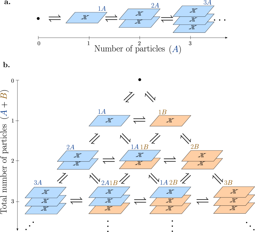
Figure 3: Structure of the phase space of the chemical diffusion master equation. a. Phase space for a system with one chemical species $A$, consisting of discrete sets of continuous diffusion domains $\mathbb{X}$ (e.g. $\mathbb{R}^{3}$), one for each particle in the current configuration. b. Analogous phase space but for a system with two chemical species $A$ and $B$. The arrows denote possible transitions between first neighbors. Reactions can in general transition between any two subsets in the phase space (not depicted).

There are also annihilation operators $a\{u_{\beta}^{*}\}$, meaning a particle is removed with rate function $u_{\beta}^{*}$, where the set $\{u^{*}_{\beta}(x)\}_{\beta\in S}$ corresponds to a basis of the dual space. These will generally correspond to bounded functions. From now on, when the argument inside the creation or annihilation operator is a basis, we will use the compact notation $a^{\dagger}_{\alpha}=a^{\dagger}\{u_{\alpha}\}$ and $a_{\beta}=a\{u_{\beta}^{*}\}$. The subtle mathematical issues related to the basis and its dual are covered in detail in [179]. The discrete lattice case from Eq. 137 is recovered by using an approximate finite basis of $L^{1}(\mathbb{X})$, such as indicator functions in voxels normalized by their volume. These do not only integrate to one (so can be interpreted as probability densities), but they also span a subspace of $L^{1}$. This case will be covered in detail in Section IV.5 and it often provides helpful insight into these representations. Also note one can also add particles with an arbitrary probability density, as later shown in Eq. 145, e.g. using a linear combination such as $(\frac{1}{2}a^{\dagger}_{\alpha}+\frac{1}{2}a^{\dagger}_{\beta})|0>$, which adds a particle with probability density $(u_{\alpha}(x)+u_{\beta}(x))/2$.

Lets consider now a system of many stochastic particles of the same species in a finite domain $\mathbb{X}$. The configuration of the system is given by the numbers of particles and their positions. The interactions between particles are capable of not only changing the spatial configuration of the particles but also the number of particles. The probability distribution $\rho$ of such a system can be expressed as

$$\rho=\left(\rho_{0},\rho_{1}(x^{(1)}),\rho_{2}(x^{(2)}),\dots,\rho_{n}(x^{(n)}),\dots\right),$$ (139)

where $\rho_{n}$ is the probability density of finding $n$ particles at positions $x^{(n)}=(x_{1}^{(n)},\dots,x_{n}^{(n)})$ with $x_{i}^{(n)}$ the position of the $i$th particle in the ensemble of $n$ particles. If clear from context, we will at times use the simplified notation: $\mathbf{x}=x^{(n)}$ and $x_{i}=x_{i}^{(n)}$. We further assume each of these densities is symmetric in its arguments since the particles are statistically indistinguishable from each other. The normalization condition is:

$$\rho_{0}+\sum_{n=1}^{\infty}\int_{\mathbb{X}^{n}}\mathbf{dx}\,\rho_{n}(\mathbf{x})=1\,,$$ (140)

with each $\mathbf{x}\in\mathbb{X}^{n}$. In general $\rho$ will also depend on time and live in a phase space with a complex structure, as depicted in Fig. 3.

We can express the state of the system using the copy number representation. The state of the system is $|\rho\rangle$, which is a linear combination of the Fock space basis elements $|\mathbf{n}\rangle$ weighted by the probabilities $p_{\mathbf{n}}$ of each configuration $\mathbf{n}$

$$|\rho\rangle= \sum_{\mathbf{n}}p_{\mathbf{n}}|\mathbf{n}\rangle,$$ (141)

where the sum is over all possible combinations of $\mathbf{n}$. The relation between the copy number representation and the classical $n$ particle densities is given by

$$|\rho_{m}(\mathbf{x})\rangle =\sum_{\mathbf{n}\in\mathbb{M}_{m}}p_{\mathbf{n}}|\mathbf{n}\rangle,$$ (142)

where $\displaystyle\mathbb{M}_{m}=\left\{\mathbf{n}=(n_{1},n_{2},...):\sum_{\alpha\in S}n_{\alpha}=m\right\}$ and thus

$$|\rho\rangle=\sum_{m\geq 0}\sum_{\mathbf{n}\in\mathbb{M}_{m}}p_{\mathbf{n}}|\mathbf{n}\rangle=\sum_{m\geq 0}|\rho_{m}(\mathbf{x})\rangle,$$ (143)

which is equivalent to Eq. 141. To provide a precise connection to the scalar probability densities from Eq. 139, it is often convenient to expand $|\rho_{m}(\mathbf{x})\rangle$ in a different basis than the copy number representation: $|\rho_{m}(\mathbf{x})\rangle=\rho_{m}(\mathbf{x})|\hat{e}_{m}\rangle$, where $|\hat{e}_{m}\rangle=(0,\dots,0,1,0,\dots)$ with $1$ in the $m$th entry and zero elsewhere. We refer to $\{|\hat{e}_{m}\rangle\}$ as the standard basis. Also note that the normalization from Eq. 140 corresponds to $\sum_{\mathbf{n}}p_{\mathbf{n}}=1$ in the copy number representation.

We can now more precisely define what we mean by Fock space in this context. The densities $\rho_{n}(x^{(n)})$ reside in a symmetrized $L^{1}(\mathbb{X})^{\otimes n}$ space, which we denote by $W_{n}$. Then, the Fock space is:

$$F:=\bigoplus_{n=0}^{\infty}W_{n}=\{\rho=(\rho_{0},\rho_{1},\dots):\rho_{n}\in W_{n}\text{ for all }n\},$$ (144)

In bra-ket notation, the direct sum can be understood in terms of a sum over the standard basis: $|\rho\rangle\in F$ can be expanded as $|\rho\rangle=\sum\rho_{n}|\hat{e}_{n}\rangle$. The distributions $\rho$ are assumed normalized following Eq. 140. In the next subsection, we will cover in detail the creation/annihilation operators and their properties, as well as other aspects including the conditions a dual basis should satisfy. Note in this setting $F$ is not necessarily a Hilbert space, but it still holds similar properties. For details on the topic, the reader is referred to [179].

IV.2 Creation and annihilation operators

In general, the creation operator adds a particle with probability density function $w:=w(x)$, and the annihilation operator removes a particle with a rate function $f:=f(x)$. For convenience, we express explicitly the action of the creation and annihilation operators on $|\rho_{n}\rangle$ here:

$$a^{\dagger}\{w\}|\rho_{n}\rangle =\frac{1}{n+1}\sum_{j=1}^{n+1}w(x_{j})\ |\rho_{n}(\mathbf{x}_{\setminus\{j\}})\rangle\,,\quad\mathbf{x}\in\mathbb{X}^{n+1},$$ (145a)

$$a\{f\}|\rho_{n}\rangle =n\int_{\mathbb{X}}f(y)\ |\rho_{n}(y,\mathbf{x})\rangle\ dy\,,\quad\mathbf{x}\in\mathbb{X}^{n-1},$$ (145b)

where $x_{j}$ correspond to the $j$th entry of the tuple $\mathbf{x}$ and $\mathbf{x}_{\setminus\{j\}}$ means that the entry with index $j$ is excluded from the tuple $\mathbf{x}$. Here $w$ is an arbitrary probability density for one particle and $f$ is an arbitrary rate function; they are not necessarily elements of the basis and its dual. In particular, when applied to basis elements of the copy number representation $|\mathbf{n}\rangle$ (or their duals), we obtain them in their basis-independent form (analogous to Eqs. 10 and 11):

$$\begin{aligned} a^{\dagger}_{\alpha^{\prime}}|\mathbf{n}\rangle&=\prod_{\alpha}(a^{\dagger}_{\alpha})^{n_{\alpha}+\delta_{\alpha\alpha^{\prime}}}\ |0\rangle,\\ a_{\beta}|\mathbf{n}\rangle&=n_{\beta}\prod_{\alpha}(a^{\dagger}_{\alpha})^{n_{\alpha}-\delta_{\alpha\beta}}\ |0\rangle.\end{aligned}$$ (146)

Naturally if $n_{\beta}=0$, then $a_{\beta}|\mathbf{n}\rangle=0$. These generalized creation and annihilation operators satisfy the following commutation relations, which is a generalization of Eq. 12:

$$\begin{aligned} \left[a\{f\},a^{\dagger}\{w\}\right]&=\langle f,w\rangle\mathcal{I}\,,\\ \left[a^{\dagger}\{w\},a^{\dagger}\{\nu\}\right]&=\Big{[}a\{f\},a\{g\}\Big{]}=0\,.\end{aligned}$$ (147)

Here $\mathcal{I}$ is the identity operator and the dual pairing (a generalization of the inner product) is defined as:

$$\langle f,w\rangle=\int_{\mathbb{X}}f(x)w(x)dx\,.$$ (148)

This definition is analogous for components in higher dimensions (integral over $\mathbb{X}^{n}$) or no integration at all if $n=0$. Through this pairing, we can obtain the dual basis. If the basis of $L^{1}$ is the set $\{u_{\alpha}(x)\}$, the basis of the dual space $\{u_{\beta}^{*}(x)\}$ satisfies the following orthonormality condition:

$$\langle u_{b}^{*},u_{\alpha}\rangle=\delta_{\alpha,\beta}\,,$$ (149)

which together with the first commutation relation from Eq. 147 yields the commutator in terms of basis elements $\left[a_{\beta},a^{\dagger}_{\alpha}\right]=\delta_{\alpha,\beta}$. Moreover, similarly to Eqs. 9 and 15, the vacuum state satisfies the following relations:

$$a\{f\}|0\rangle=0\,,\ \quad\langle 0|a^{\dagger}\{w\}=0\,,\ \quad\ \langle 0|0\rangle=1\,,$$ (150)

which also apply in the special case where $f$ is $u_{\alpha}$ and $w$ is $u_{\beta}^{*}$. We can now generalize the copy number representation from Eq. 138 to include its dual, as in (15):

$$|\mathbf{n}\rangle=\prod_{\alpha}(a^{\dagger}_{\alpha})^{n_{\alpha}}|0\rangle,\quad\langle\mathbf{n}|=\langle 0|\frac{1}{\mathbf{n}!}\prod_{\beta}(a_{\beta})^{n_{\beta}}$$ (151)

with $\mathbf{n}!=\prod_{\beta}n_{\beta}!$. One can intuitively understand the $\mathbf{n}!$ as a normalizing factor to take into account all the equivalent ways of removing $n$ particles of the same species from a symmetric density. Combining Eq. 151 with the properties from Eqs. 147 and 150 and the orthogonality of the basis, we can show the orthogonality of the Fock space basis in terms of bras and kets

$$\langle\mathbf{n}|\mathbf{m}\rangle=\prod_{\alpha}\ \delta_{m_{\alpha},n_{\alpha}}=\delta_{\mathbf{n},\mathbf{m}}.$$ (152)

The coherent states and their duals are

$$|\mathbf{z}\rangle =\exp\left(\sum_{\alpha}z_{\alpha}a^{\dagger}_{\alpha}\right)|0\rangle\,,$$ (153a)

$$\langle\mathbf{z}| =\langle 0|\exp\left(\sum_{\beta}z_{\beta}a_{\beta}\right)\,,$$ (153b)

such that $a_{\beta}|\mathbf{z}\rangle=z_{\beta}|\mathbf{z}\rangle$ and $\langle\mathbf{z}|a^{\dagger}_{\alpha}=z_{\alpha}\langle\mathbf{z}|$, i.e. the coherent states are eigenstates of the creation and annihilation operators, respectively. This can be shown by direct substitution and use of the commutation relations Eq. 147.

IV.2.1 Generating functions and number operators

In Section II.5, we discussed the generating function approach to master equations; here we obtain an analogous result by following the same procedure. From the definition of coherent state in (153), we can show that

$$\langle\textbf{z}|a_{\alpha}^{\dagger}=z_{\alpha}\langle\textbf{z}|,\quad\text{and}\quad\langle\textbf{z}|a_{\alpha}=\frac{d}{dz_{\alpha}}\langle\textbf{z}|.$$ (154)

Assuming an evolution of a system with one chemical species generated by a generator $H$ expanded in terms of creation and annihilation operators $H:=H(\textbf{a}^{\dagger},\textbf{a})$, we can derive an evolution for the generating function $G(\textbf{z})=\langle\textbf{z}|p\rangle$ as previously and obtain $\frac{d}{dt}G(\textbf{z})=H(\textbf{z},\frac{d}{d\textbf{z}})G(\textbf{z})$, where in this case each variable $z_{\alpha}$ of the equation is associated to one of the basis functions rather than to one chemical species. We can again use the coherent state $\langle\mathbf{1}|$ to calculate expectations; it corresponds to $z_{\alpha}=1$ for all $\alpha$’s: $\langle\mathbf{1}|=\langle 0|\exp\left(\sum_{\alpha}a_{\alpha}\right)$. Other properties are also analogous to the expressions for the well-mixed case, like the number operators

$$\mathcal{N}_{\alpha}=a^{\dagger}_{\alpha}a_{\alpha}\qquad\mathcal{N}=\sum_{\alpha}a^{\dagger}_{\alpha}a_{\alpha},$$ (155)

such that $\mathcal{N}_{\alpha}|\rho\rangle=n_{\alpha}|\rho\rangle$ and $\mathcal{N}|\rho\rangle=\left(\sum_{\alpha}n_{\alpha}\right)|\rho\rangle$. All these results can be analogously extended to systems involving two or more chemical species.

IV.3 The chemical diffusion master equation

The chemical diffusion master equation (CDME) is the master equation for reaction-diffusion processes. We use this name since the name reaction-diffusion master equation is normally reserved for discrete space settings, see Fig. 1. To construct this equation, we need to write the generator of the underlying reaction-diffusion process as a combination of different operators acting on the Fock space elements. For a reaction-diffusion system with one chemical species and $R$ reactions, the generator of the master equation is

$$H=H_{0}(D)+\sum_{r=1}^{R}H_{r}(\lambda_{r}),$$ (156)

where $H_{0}(D)$ is the diffusion operator and $H_{r}(\lambda_{r})$ are the reaction operators corresponding to the $r$-th reaction with rate function $\lambda_{r}$. Using this generator, we can write the CDME using kets

$$\partial_{t}|\rho\rangle=H|\rho\rangle.$$ (157)

The equation doesn’t need to be written in bra-ket notation; it can also be written in a standard form, as shown in Section V.3 and [179, 182, 68]. The phase space of the CDME is illustrated in Fig. 3 for systems with one and two chemical species, which illustrates the complexity of the underlying Fock space.

Some of the operators in Eq. 156 will not change the number of particles, such as diffusion operators, while some others will, like reaction operators. All these operators can be expressed in terms of creation and annihilation operators, which we will show in the next subsections. In particular, we show how to expand the diffusion operator and the reaction operator for a general one species reaction and how it extends to reactions with multiple species.

IV.3.1 Particle number conserving operators

Lets focus first on operators that do not change the number of particles. Consider an operator $A$ acting on a single particle, such that $A:L^{1}(\mathbb{X})\to L^{1}(\mathbb{X})$; the action of this operator on the whole system (i.e. on the Fock space) can be expressed as an operator $F_{A}$, which has a representation in terms of creation and annihilation operators

$$F_{A}=\sum_{\alpha,\beta}\langle u_{\alpha}^{*},Au_{\beta}\rangle a^{\dagger}_{\alpha}a_{\beta}.$$ (158)

This equation was proved in [179, 182], and it is not trivial. However, we can still gain some additional insight and intuition by focusing on a specific case. For instance, the diffusion operator $D\nabla^{2}$ doesn’t change the number of particles and acts on a single particle. Its action on the whole Fock space is expressed as the operator

$$H_{0}(D)=\sum_{\alpha,\beta}\langle u_{\alpha}^{*},D\nabla^{2}u_{\beta}\rangle a^{\dagger}_{\alpha}a_{\beta},$$ (159)

so it belongs to the representation in the form of Eq. 158. To intuitively understand this equation, let’s think once again of a lattice discretization, where we make a full partition of space and each $u_{\alpha}$ represents a normalized indicator function. Then each term in Eq. 159 represents the action of removing one particle from site $\beta$ and adding it into site $\alpha$ in the lattice. The quantity $\langle u_{\alpha}^{*},\nabla^{2}u_{\beta}\rangle$ denotes how much probability should be transferred between voxels $\alpha$ and $\beta$ by this action, and it will only be non-zero between neighboring voxels. To obtain the action of the operator on the whole system, we must sum over all possible voxel combinations $(\alpha,\beta)$.

We can also have operators $B$ that act on two particles at a time, $B:L^{1}(\mathbb{X})^{\otimes 2}\to L^{1}(\mathbb{X})^{\otimes 2}$, such as diffusion with pair interactions through a potential. We can extend Eq. 158 as:

$$F_{B}=\sum_{\bm{\alpha},\bm{\beta}\in S^{2}}\langle u^{*}_{\bm{\alpha}},Bu_{\bm{\beta}}\rangle a^{\dagger}_{\bm{\alpha}}a_{\bm{\beta}},$$ (160)

where we used the compact notation $u_{\bm{\beta}}(\mathbf{x})=u_{\beta_{1}}(x_{1})\otimes u_{\beta_{2}}(x_{2})$ for the basis of $L^{1}\otimes L^{1}$; $u^{*}_{\bm{\alpha}}(\mathbf{x})=u^{*}_{\alpha_{1}}(x_{1})\otimes u^{*}_{\alpha_{2}}(x_{2})$ for the basis of the dual; $a^{\dagger}_{\bm{\alpha}}=a^{\dagger}_{\alpha_{1}}a^{\dagger}_{\alpha_{2}}$ and $a_{\bm{\beta}}=a_{\beta_{1}}a_{\beta_{2}}$. We assumed $B$ is symmetric under particle permutations. We can use analogous expansions for operators $Z:L^{1}(\mathbb{X})^{\otimes m}\to L^{1}(\mathbb{X})^{\otimes m}$ acting on $m$ permutation symmetric particles at a time

$$F_{Z}=\sum_{\bm{\alpha},\bm{\beta}\in S^{m}}\langle u^{*}_{\bm{\alpha}},Zu_{\bm{\beta}}\rangle a^{\dagger}_{\bm{\alpha}}a_{\bm{\beta}},$$ (161)

where we generalized the compact notation to $\bm{\alpha}=(\alpha_{1},...,\alpha_{m})\in S^{m}$, $\bm{\beta}=(\beta_{1},...,\beta_{m})\in S^{m}$ and $\mathbf{x}=(x_{1},...,x_{m})\in\mathbb{X}^{m}$ with

$$\begin{aligned} u_{\bm{\beta}}(\mathbf{x})&=u_{\beta_{1}}(x_{1})\otimes...\otimes u_{\beta_{m}}(x_{m}),\\ u^{*}_{\bm{\alpha}}(\mathbf{x})&=u^{*}_{\alpha_{1}}(x_{1})\otimes...\otimes u^{*}_{\alpha_{m}}(x_{m}).\end{aligned}$$ (162)

and $a^{\dagger}_{\bm{\alpha}}=a^{\dagger}_{\alpha_{1}}\cdots a^{\dagger}_{\alpha_{n}}$ and $a_{\bm{\beta}}=a_{\beta_{1}}\cdots a_{\beta_{m}}$.

IV.3.2 Reaction operators

Reaction events will in general change the number of particles; however, they must still conserve the total probability. The reaction operator $H(\lambda)$ for a given reaction with rate function $\lambda$ is split into two operators:

$$H(\lambda)=\mathcal{G}-\mathcal{L}.$$ (163)

As before, the gain $\mathcal{G}$ quantifies how much probability is being “gained” by the current state from another state due to the reaction. Similarly, the loss quantifies how much probability is being “lost” by the current state, as it is required to ensure that probability is conserved. The gain operator does not conserve particle numbers, while the loss does and thus belongs to the class of operators presented in Section IV.3.1. The separation into these two terms is analogous to the two terms in Eq. 31. To simplify the presentation, lets focus first on examples involving only one chemical species.

General one species reaction

Consider the most general reaction of a system with only one chemical species:

$$kA\rightarrow\ell A$$ (164)

with space-dependent rate function $\lambda(\mathbf{y};\mathbf{x})$, where $\mathbf{x}\in\mathbb{X}^{k}$ are the positions of the reactants and $\mathbf{y}\in\mathbb{X}^{\ell}$ the positions of the corresponding products. As the particles are indistinguishable, the rate function must be symmetric with respect to permutations of the reactants positions, as well as permutations of the products positions.

To construct the reaction operator, we write the per reaction loss operator, $L:L^{1}(\mathbb{X})^{\otimes k}\to L^{1}(\mathbb{X})^{\otimes k}$ and gain operator $G:L^{1}(\mathbb{X})^{\otimes k}\to L^{1}(\mathbb{X})^{\otimes\ell}$ , which are defined on the $k$ particle space basis functions $u_{\bm{\beta}}$ and written in terms of the reaction rate function, namely

$$\begin{aligned} \bigl{(}Lu_{\bm{\beta}}\bigr{)}(\mathbf{x}):=&u_{\bm{\beta}}(\mathbf{x})\int_{\mathbb{X}^{\ell}}d\mathbf{y}\;\lambda(\mathbf{y};\mathbf{x}),\\ \bigl{(}Gu_{\bm{\beta}}\bigr{)}(\mathbf{y}):=&\int_{\mathbb{X}^{k}}\mathbf{dx}\;\lambda(\mathbf{y};\mathbf{x})u_{\bm{\beta}}(\mathbf{x}).\end{aligned}$$ (165)

Both the loss and the gain are probability fluxes, given by the product of the rate function times a probability density of the reactants given by $u_{\bm{\beta}}$. As the loss represents the loss of probability due to one reaction from the current state to any other state, it is integrated over all product positions and it depends only on the positions of the reactants. The gain function signifies the “gain” of probability due to one reaction into the current state and is hence integrated over the reactants positions, leaving a function of only the products locations. The total loss and gain over all possible reactions in the system can also be obtained by expanding in terms of creation and annihilation operators [179, 182]

$$\begin{aligned} \mathcal{L}&=\frac{1}{k!}\sum_{\begin{subarray}{c}\bm{\alpha}\in S^{k}\\ \bm{\beta}\in S^{k}\end{subarray}}\langle u_{\bm{\alpha}}^{*},Lu_{\bm{\beta}}\rangle a_{\bm{\alpha}}^{\dagger}a_{\bm{\beta}}\ ,\\ \mathcal{G}&=\frac{1}{k!}\sum_{\begin{subarray}{c}\bm{\alpha}\in S^{\ell}\\ \bm{\beta}\in S^{k}\end{subarray}}\langle u_{\bm{\alpha}}^{*},Gu_{\bm{\beta}}\rangle a_{\bm{\alpha}}^{\dagger}a_{\bm{\beta}}\ ,\end{aligned}$$ (166)

where these operators now act on the Fock space. The reaction operator for this reaction is $H(\lambda)=\mathcal{G}-\mathcal{L}$; the diagram in Fig. 4 illustrates its construction. For insight, we can understand the gain as removing $k$ particles and adding $\ell$ particles, weighted by the rate function and summing over all possible combinations. If applied to $|\rho_{n+k-l}\rangle$, it yields the probability gain into the $n$ state. The loss applied to $|\rho_{n}\rangle$ quantifies how the probability to remain in the current state decreases, ensuring the total probability is conserved.

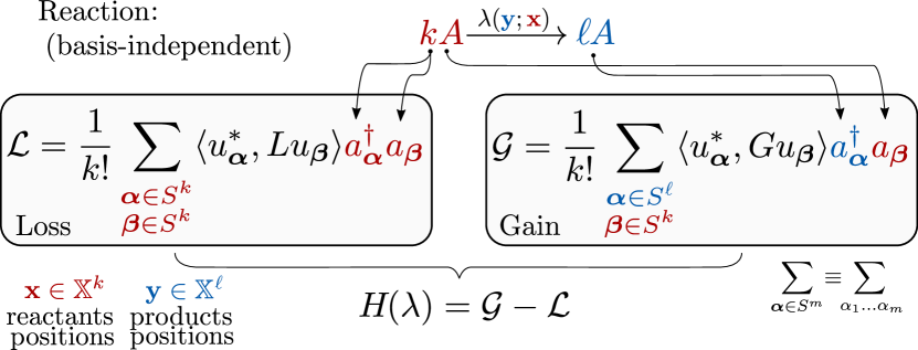
Figure 4: Diagram illustrating how to construct the generator for a system with a general one species reaction with rate function $\lambda(\mathbf{y};\mathbf{x})$ for the basis-independent case. Note this case takes into account the spatial dynamics in continuous space, so it generalizes the diagram presented for the well-mixed case, (Fig. 2).

Degradation and creation reactions

As special cases, we can write the generators for degradation and creation reactions. Let us first consider a degradation reaction $A\rightarrow\emptyset$ that occurs with spatially-dependent rate function $\lambda_{d}(x)$. The loss and gain per reaction are special cases of Eq. 165

$$\begin{aligned} \left(L_{d}u\right)(x)&=u(x)\lambda_{d}(x),\\ \left(G_{d}u\right)&=\int_{\mathbb{X}}u(y)\lambda_{d}(y)dy.\end{aligned}$$ (167)

Analogously, the loss and gain operators acting on the whole system (the Fock space) are special cases of Eq. 166, and thus the full system reaction operator due to a degradation reaction is given by $H_{d}(\lambda_{d})=\mathcal{G}_{d}-\mathcal{L}_{d}$, i.e.

$$H_{d}(\lambda_{d})=\sum_{\beta}\langle 1,G_{d}u_{\beta}\rangle a_{\beta}-\sum_{\alpha,\beta}\langle u_{\alpha}^{*},L_{d}u_{\beta}\rangle a^{\dagger}_{\alpha}a_{\beta}.$$ (168)

where $\langle 1,G_{d}u_{\beta}\rangle=G_{d}u_{\beta}$.

Analogously, we can consider the creation reaction $\emptyset\rightarrow A$ with spatially-dependent rate $\lambda_{c}(x)$. The loss and gain operators per reaction are

$$L_{c}=\int_{\mathbb{X}}\lambda_{c}(y)dy,\qquad G_{c}=\lambda_{c}(y),$$ (169)

such that the generator for the creation reaction is

$$H_{c}(\lambda_{c})=\sum_{\alpha}\langle u_{\alpha}^{*},G_{c}1\rangle a^{\dagger}_{\alpha}-L_{c}.$$ (170)

IV.4 Extension to multiple species

The extension of this formalism to systems with multiple chemical species in straightforward, however, the notation can become cumbersome. So instead of presenting the most general case, we focus on a simple bimolecular reaction

$$A+B\rightarrow C,$$ (171)

with rate function $\lambda(y_{c};x_{a},x_{b})$, where $x_{a}$ and $x_{b}$ are the locations of the reactants and $y_{c}$ is the location of the product. The key to write the corresponding generator is to use different creation and annihilation operators for each species. The creation and annihilation operators for each species are denoted by the corresponding lower case letter. Analogously to Eq. 165, the loss and gain operators per reaction are given in terms of the rate function $\lambda$ as

$$\begin{aligned} \big{(}Lu_{\bm{\beta}}\big{)}(x_{a},x_{b})&:=u_{\bm{\beta}}(x_{a},x_{b})\int_{\mathbb{X}}\lambda(y_{c};x_{a},x_{b})dy_{c},\\ \big{(}Gu_{\bm{\beta}}\big{)}(y_{c})&:=\int_{\mathbb{X}^{2}}u_{\bm{\beta}}(x_{a},x_{b})\lambda(y_{c};x_{a},x_{b})dx_{a}dx_{b},\end{aligned}$$ (172)

with $u_{\bm{\beta}}=u_{\beta_{1}}\otimes u_{\beta_{2}}$ to shorten notation. Analogously to the previous sections, the total loss and gain terms take the following expansions [179]:

$$\mathcal{L} =\frac{1}{2}\sum_{\begin{subarray}{c}\alpha_{1},\alpha_{2}\\ \beta_{1},\beta_{2}\end{subarray}}\left\langle u_{\alpha_{1}}^{*}\otimes u_{\alpha_{2}}^{*},L(u_{\beta_{1}}\otimes u_{\beta_{2}})\right\rangle a^{\dagger}_{\alpha_{1}}b^{\dagger}_{\alpha_{2}}a_{\beta_{1}}b_{\beta_{2}},$$

$$\mathcal{G} =\frac{1}{2}\sum_{\begin{subarray}{c}\alpha\\ \beta_{1},\beta_{2}\end{subarray}}\left\langle u_{\alpha}^{*},G(u_{\beta_{1}}\otimes u_{\beta_{2}})\right\rangle c^{\dagger}_{\alpha}a_{\beta_{1}}b_{\beta_{2}},$$ (173)

where $a^{\dagger},b^{\dagger},c^{\dagger},a,b,c$ correspond to creation and annihilation of particles of type $A,B$ and $C$ correspondingly. If these are from different species, they commute; if not, they follow the usual commutation relations (Eq. 147). Once again the generator for the reaction is $H(\lambda)=\mathcal{G}-\mathcal{L}$, and the full generator includes the diffusion of each chemical species, thus

$$H=H_{0}(D_{A})+H_{0}(D_{B})+H_{0}(D_{C})+H(\lambda),$$ (174)

with $D_{A}$, $D_{B}$ and $D_{C}$ the diffusion coefficients of each species. This case and others were studied in detail in [182], where it is also shown how to recover the standard integro-differential form from this representation.

IV.5 Galerkin discretization: indicator functions as basis

In Section IV.1, we introduced the basis-independent continuous formulation of stochastic reaction-diffusion processes. In this section, following the results from [179], we show that starting from the continuous formulation, we can not only consistently recover the second quantized representation of reaction-diffusion on the lattice used in Sections III.1 and III.2 but also derive any arbitrary discretization in the field theory representation, yielding the second quantized Galerkin discretization from Fig. 1. The probability distribution $\rho$ (Eq. 139) is a high-dimensional object; it depends on all the possible number of particles and all their positions. The goal of discretizing it is to simplify the problem by reducing its dimensionality and to make it accessible for numerical implementations.

We begin by applying a piecewise constant approximation on the whole space. Let us consider a partition of the full space where the particles reside in $M$ non-overlapping subsets denoted by $\mathbb{X}_{i}$ with $i=1,\dots,M$ (in the lattice case, each $\mathbb{X}_{i}$ corresponds to a voxel). The indicator function $\mathbb{1}_{\mathbb{X}_{i}}$ has value $1$ in $\mathbb{X}_{i}$ and $0$ elsewhere. These indicator functions form a basis of a subspace of $L^{1}$ —the space of integrable functions that are piecewise constant on all $\mathbb{X}_{i}$’s. For convenience, we use the normalized indicator functions as a basis of the discretized space

$$\xi_{i}=\frac{\mathbb{1}_{\mathbb{X}_{i}}}{||\mathbb{1}_{\mathbb{X}_{i}}||},$$ (175)

where $||\mathbb{1}_{\mathbb{X}_{i}}||$ is the volume of $\mathbb{X}_{i}$. Thus, the space integral of $\xi_{i}$ is always one. We further denote $\xi_{j}^{*}$ as the dual of the basis $\xi_{j}$, which corresponds to $\xi_{j}^{*}=\mathbb{1}_{\mathbb{X}_{j}}$, so the orthonormality condition is satisfied $\langle\xi_{i}^{*}|\xi_{j}\rangle=\delta_{ij}$.

Based on the expressions from Section IV.2, we obtain the creation and annihilation operators $a_{i}^{\dagger}$ and $a_{j}$, which correspond to creating or annihilating a particle on set/region $\mathbb{X}_{i}$ by their action on the corresponding basis elements

$$a_{i}^{\dagger}:=a^{\dagger}\{\xi_{i}\}\qquad a_{j}:=a\{\xi_{j}^{*}\}.$$ (176)

The copy number representation is analogous to Eq. 151, with the main difference that the basis is finite:

$$\begin{split}|\mathbf{n}\rangle:&=|n_{1},...,n_{M}\rangle\\ &=(a^{\dagger}_{1})^{n_{1}}...(a^{\dagger}_{M})^{n_{M}}|0\rangle\,.\end{split}$$ (177)

Hence, there are $n_{i}$ particles in region $\mathbb{X}_{i}$. The action of the creation and annihilation operators on these states follows from Eq. 146

$$\begin{split}a^{\dagger}_{i}|\mathbf{n}\rangle&=|n_{1},..,n_{i}+1,..,n_{M}\rangle\,,\\ a_{j}|\mathbf{n}\rangle&=n_{j}\ |n_{1},..,n_{j}-1,..,n_{M}\rangle\,.\end{split}$$ (178)

These expressions are similar to Eqs. 11 and 10, with the difference that here we do not distinguish the species, but its location in discretized space. An expression for the discretized density $\hat{\rho}$ is analogous to Eq. 141

$$\hat{\rho}=\sum_{\mathbf{n}}p_{\mathbf{n}}|\mathbf{n}\rangle,\$$ (179)

where $p_{\mathbf{n}}$ is simply the probability of configuration $\mathbf{n}=(n_{1},...,n_{M})$, i.e. the probability of having $n_{i}$ particles in set $\mathbb{X}_{i}$ for $i=1,...,M$. Next, we want to discretize the operators that act on the density by projecting into the discretized subspace. We start with the diffusion operator. Using Eq. 159, we substitute the basis $u_{\alpha}$ with the basis of the subspace $\xi_{i}$ and similarly for $u_{\beta}^{*}$

$$H_{0}(D)=\sum_{i,j=1}^{M}D_{ij}a^{\dagger}_{i}a_{j}\,,$$ (180)

with $D_{ij}=\langle\xi_{i}^{*},D\nabla^{2}\xi_{j}\rangle$. To compute $D_{ij}$ explicitly, one has to interpret it in the distributional sense. Lets calculate this explicitly in one dimension, such that $||\mathbb{1}_{\mathbb{X}_{i}}||=h$, and apply it to a test function, $\phi(x)$. For a fixed $i$, the sum over $j$ of these terms yields

$$\sum_{j=1}^{M}D_{ij}\phi(x)=\sum_{j=1}^{M}\langle\xi_{i}^{*},D\partial_{x}^{2}(\xi_{j}\phi(x))\rangle$$

$$\ =\sum_{j=1}^{M}\frac{D}{h}\int_{\mathbb{X}_{i}}\partial_{x}^{2}(\mathbb{1}_{\mathbb{X}_{j}}\phi(x))dx=\frac{D}{h}\partial_{x}(\mathbb{1}_{\mathbb{X}_{i}}\phi(x))\Big{|}_{x_{i-1/2}}^{x_{i+1/2}}$$

$$\ =\frac{D}{h}\left(\phi^{\prime}(x_{i+1/2})-\phi^{\prime}(x_{i-1/2})\right)$$

$$\ =\frac{D}{h^{2}}\left(\phi_{i+1}+\phi_{i-1}-2\phi_{i}\right)+O(h^{2}),$$ (181)

where in the last line, we used a piecewise constant discretization of the test function in the same lattice to approximate the derivatives. This shows that in a 1D lattice, we can interpret the coefficients as $D_{ii}=-2D/h^{2}$ and $D_{ij}$ will be $D/h^{2}$ for $j=i\pm 1$ and zero otherwise, similar to Eq. 70. One can extend the calculation to higher dimensions and non-lattice discretizations. In general, $D_{ij}$ will be non-zero only for $i,j$ nearest neighbors and $D_{ii}=-\sum_{i\neq j}D_{ji}$, such that $D$ is the graph Laplacian of the discretization. We can apply $H_{0}(D)$ to $\hat{\rho}$ by using Eq. 178,

$$H_{0}(D)\hat{\rho}=\sum_{i,j=1}^{M}D_{ij}a^{\dagger}_{i}a_{j}\sum_{\mathbf{n}}p_{\mathbf{n}}|\mathbf{n}\rangle$$

$$=\sum_{\mathbf{n}}\left(\sum_{\begin{subarray}{c}{i,j=1}\\ i\neq j\end{subarray}}^{M}D_{ij}n_{j}p_{\mathbf{n}}|\mathbf{n}_{i+1,j-1}\rangle+\sum_{i=1}^{M}D_{ii}n_{i}p_{\mathbf{n}}|\mathbf{n}\rangle\right)$$

$$=\sum_{\mathbf{n}}\left(\sum_{\begin{subarray}{c}{i,j=1}\\ i\neq j\end{subarray}}^{M}D_{ij}(n_{j}+1)p_{\mathbf{n}_{i-1,j+1}}+\sum_{i=1}^{M}D_{ii}n_{i}p_{\mathbf{n}}\right)|\mathbf{n}\rangle$$

$$=\sum_{\mathbf{n}}\tilde{H}_{0}(D)p_{\mathbf{n}}|\mathbf{n}\rangle$$ (182)

with $|\mathbf{n}_{i+1,j-1}\rangle:=|n_{1},..,n_{i}+1,..,n_{j}-1,..,n_{M}\rangle$ and $p_{\mathbf{n}_{i-1,j+1}}:=p_{n_{1},..,n_{i}-1,..,n_{j}+1,..,n_{M}}$ for compact notation and where $\tilde{H}_{0}(D)$ is the diffusion operator acting on the coefficients/probabilities $p_{\mathbf{n}}$, i.e.

$$\tilde{H}_{0}(D)p_{\mathbf{n}} =\sum_{\begin{subarray}{c}{i,j=1}\\ i\neq j\end{subarray}}^{M}\left(D_{ij}(n_{j}+1)p_{\mathbf{n}_{i-1,j+1}}-D_{ji}n_{i}p_{\mathbf{n}}\right).$$ (183)

Where we have used that $D_{ii}=-\sum_{i\neq j}D_{ji}$.

Applying this discretization process for the diffusion master equation, yields immediately a master equation for the discretized diffusion process in terms of the coefficients/probabilities $p_{\mathbf{n}}$,

$$\partial_{t}p_{\mathbf{n}}=\tilde{H}_{0}(D)p_{\mathbf{n}}.$$ (184)

In the case of a lattice, one recovers the usual finite difference discretization of the diffusion equation. Applying an analogous approach to the expansions for the loss and gain operators for the degradation reaction from Eq. 168, we also obtain the discretized operators acting directly on the coefficients/probabilities $p_{\mathbf{n}}$:

$$\tilde{H}_{d}(\lambda_{d})\ p_{\mathbf{n}}=\sum_{i=1}^{M}\lambda_{d}^{i}\left((n_{i}+1)p_{n_{1},..,n_{i}+1,..,n_{M}}-n_{i}p_{\mathbf{n}}\right)\,,$$ (185)

with $\lambda_{d}^{i}=\langle\xi_{i}^{*},L_{d}\xi_{i}\rangle=\langle 1,G_{d}\xi_{i}\rangle=\int\lambda_{d}(x)\xi_{i}(x)dx$. Analogously, the creation reaction from Eq. 170 becomes:

$$\tilde{H}_{c}(\lambda_{c})\ p_{\mathbf{n}} =\sum_{i=1}^{M}\lambda_{c}^{i}\left(p_{n_{1},..,n_{i}-1,..,n_{M}}-p_{\mathbf{n}}\right)\,,$$ (186)

with $\lambda_{c}^{i}=\langle\xi_{i}^{*},G_{c}1\rangle=\int\xi_{i}^{*}(x)\lambda_{c}(x)dx$. The master equation for discretized reaction-diffusion process with creation and degradation reactions is then

$$\partial_{t}p_{\mathbf{n}}=\left(\tilde{H}_{0}(D)+\tilde{H}_{d}(\lambda_{d})+\tilde{H}_{c}(\lambda_{c})\right)p_{\mathbf{n}},$$ (187)

which is the so-called reaction-diffusion master equation (a spatially discretized CDME). One can also discretize more complex reaction operators, including bimolecular reactions, whose rate function depend on the intermolecular distance or other non-linear parameters. In these cases, this discretization approach guarantee consistent and convergent results regardless of the chosen discretization (lattice/voxel size) [179, 114], see also Section IV.6. The discretized equations are suitable for numerical implementations, as implemented in many software packages (e.g. [17, 71]).

The field theory representation for the well-mixed case from Section II.2 is recovered when choosing a basis that covers the whole domain $\mathbb{X}$, e.g. $\mathbb{X}/||\mathbb{X}||$ (see Fig. 1). However, for nonlinear reactions, the effective rates in the well-mixed theory do not necessarily match the spatial dependent rates in the continuous theory. These relations are in general not trivial due to diffusion-influenced phenomena, see [177, 69] for a discussion on this topic.

Galerkin discretizations are not limited to this choice of basis functions nor to lattice discretizations. There are many other alternatives: one could choose overlapping basis functions or perhaps a subset of indicator functions as basis that only covers the metastable regions instead of the whole space $\mathbb{X}$ (recovering the so-called spatio-temporal master equation [224]). However, one must be careful as the choice of basis functions might have consequences in the normalization and positivity of the projected densities, an issue addressed in more detail in [179]. In the next section, we will show how one can construct the path integral formalism based on a generic Galerkin discretization.

IV.6 Path integrals for basis-independent discretizations

In this section, we integrate the Peliti path integral formalism into the basis-independent setting. We first apply the Galerkin method described in the previous section but without fixing a specific basis. This yields the second quantized Galerkin description in a basis-independent form. Then, we extend the path integral formalism from Section III.2 into this setting, which enables deriving a basis-independent discretized mean-field equation for the underlying stochastic process. The stochastic mesoscopic corrections can then be captured using diagrammatic techniques. However, since these are analogous to Sections III.3 and III.4, we will only hint to the computation of the propagator.

In Section IV.2, we defined annihilation and creation operators with respect to a general arbitrary basis of $L^{1}(X)$. Here we focus on a finite basis (a Galerkin discretization) such as the indicator functions in (175) but not limited to them. Let this finite basis be $\{\xi_{\alpha}\}_{\alpha\in S}$—a basis for a subspace of $L^{1}(X)$—where here $S$ is a finite set. Then, given that $||\xi_{\alpha}||_{1}=1$ and $\langle\xi_{\alpha}^{*},\xi_{\beta}\rangle=\delta_{\alpha\beta}$, the associated annihilation and creation operators satisfy the commutation relation $[a_{\alpha},a_{\beta}^{\dagger}]=\delta_{\alpha\beta}$. Similarly to the previous derivation of the path integral, we introduce coherent states, now for discretized space, let $\mathbf{z}\in\mathbb{C}^{S}$, then

$$|\mathbf{z}\rangle=\exp\left(\sum_{\alpha\in S}z_{\alpha}a^{\dagger}_{\alpha}\right)|\mathbf{0}\rangle\;,$$ (188)

as in (153). These coherent states satisfy the completeness relation

$$\frac{1}{\pi^{|S|}}\int_{\mathbb{C}^{S}}d\bar{\mathbf{z}}d\mathbf{z}\;e^{-\bar{\mathbf{z}}\mathbf{z}}|\mathbf{z}\rangle\langle\mathbf{z}|=1\;,$$ (189)

where $|S|$ is the cardinality of $S$. From here on, the derivation of the path integral action follows Section III.2, the main difference being that space is already discretized, hence the continuum limit is only applied to the temporal discretization introduced by the procedure. The loss and gain operators for the Galerkin approximation of the general one species reaction $kA\to\ell A$ can be written completely analogously to (166) with the difference that $S$ is now a finite set. Hence we obtain

$$\begin{split}\mathcal{G}&=\sum_{\begin{subarray}{c}\bm{\alpha}\in S^{\ell}\\ \bm{\beta}\in S^{k}\end{subarray}}G^{(\ell,k)}_{\bm{\alpha}\bm{\beta}}a_{\bm{\alpha}}^{\dagger}a_{\bm{\beta}},\quad\text{with}\quad G^{(\ell,k)}_{\bm{\alpha}\bm{\beta}}=\frac{1}{k!}\langle\xi_{\bm{\alpha}}^{*},G\xi_{\bm{\beta}}\rangle,\\ \mathcal{L}&=\sum_{\begin{subarray}{c}\bm{\alpha}\in S^{k}\\ \bm{\beta}\in S^{k}\end{subarray}}L^{(k)}_{\bm{\alpha}\bm{\beta}}\ a_{\bm{\alpha}}^{\dagger}a_{\bm{\beta}},\quad\ \text{with}\quad\ L^{(k)}_{\bm{\alpha}\bm{\beta}}=\frac{1}{k!}\langle\xi_{\bm{\alpha}}^{*},L\xi_{\bm{\beta}}\rangle,\end{split}$$ (190)

where we introduced the compact notation $G^{(\ell,k)}_{\bm{\alpha}\bm{\beta}}$ and $\ L^{(k)}_{\bm{\alpha}\bm{\beta}}$ that facilitates calculations later on. Note these expressions describe how the rate function inside $G$ and $L$ (Eq. 165) is discretized for any chosen finite basis, ensuring consistency across different discretizations. The reaction operator is

$$H(\lambda)=\mathcal{G}-\mathcal{L}.$$ (191)

The infinitesimal stochasticity of the reaction operator after the discretization can be expressed as

$$0=\langle\mathbf{1}|H=\langle\mathbf{1}|\sum_{\bm{\beta}\in S^{k}}a_{\bm{\beta}}\left(\sum_{\bm{\alpha}\in S^{\ell}}G^{(\ell,k)}_{\bm{\alpha}\bm{\beta}}-\sum_{\bm{\alpha}\in S^{k}}L^{(k)}_{\bm{\alpha}\bm{\beta}}\right),$$ (192)

which implies that for each $\bm{\beta}\in S^{k}$ the expression in the brackets vanishes. The same condition on the diffusion operator reads as

$$0=\langle\mathbf{1}|H_{0}(D)=\langle\mathbf{1}|\sum_{\beta\in S}a_{\beta}\left(\sum_{\alpha\in S}D_{\alpha\beta}\right),$$ (193)

implying that the finite matrix with elements $D_{\alpha\beta}$ should be infinitesimally stochastic. Thus, from the above equations, the conservation of probability implies

$$0 =\sum_{\bm{\alpha}\in S^{\ell}}G^{(\ell,k)}_{\bm{\alpha}\bm{\beta}}-\sum_{\bm{\alpha}\in S^{k}}L^{(k)}_{\bm{\alpha}\bm{\beta}},\quad\text{and}$$ (194)

$$0 =\sum_{\alpha\in S}D_{\alpha\beta},$$ (195)

since all vectors $\langle 1|a_{\bm{\beta}}$ in Eq. 192 and $\langle 1|a_{\beta}$ in Eq. 193 are linearly independent. This will be used later to simplify the path integral action after performing the Doi shift. The path integral action, similar to (III.3), now reads

$$\begin{split}S[\bar{\bm{\phi}},\bm{\phi}]&=\int dt\;s(\bar{\bm{\phi}},\bm{\phi},\partial_{t}\bm{\phi})\\ &=\int dt\;\bigl{[}\bar{\bm{\phi}}(\partial_{t}-\mathbb{D})\bm{\phi}-s_{\mathcal{R}}(\bar{\bm{\phi}},\bm{\phi})\bigr{]},\end{split}$$ (196)

where $\mathbb{D}$ is the matrix/operator with elements $D_{\alpha\beta}$ and $\bar{\bm{\phi}},\bm{\phi}:\mathbb{R}\to\mathbb{C}^{S}$, and $s_{\mathcal{R}}(\bar{\bm{\phi}},\bm{\phi})$ is obtained from $H$ with the substitution

$$a_{\beta} \mapsto\phi_{\beta},$$ (197)

$$a^{\dagger}_{\beta} \mapsto\bar{\phi}_{\beta}+1.$$ (198)

Here the shift in the second line is the Doi shift. Note that we have omitted in (196) the boundary term in the last line of (III.3), since that term will not contribute to the derivation of the mean-field equations. The form of $s_{\mathcal{R}}(\bar{\bm{\phi}},\bm{\phi})$ for the reaction $kA\to\ell A$ can be expressed in terms of the elementary symmetric polynomials in the variables $x_{j}$ for $j\in\{1,...,n\}$

$$e^{(n)}_{q}(\mathbf{x}) :=\sum_{1\leq j_{1}<\dots<j_{q}\leq n}x_{j_{1}}\dots x_{j_{k}},$$ (199)

$$e^{(n)}_{0}(\mathbf{x}) =1,$$ (200)

yielding an expression for the action

$$\begin{split}s_{\mathcal{R}}(\bar{\bm{\phi}},\bm{\phi})&=\sum_{\begin{subarray}{c}\bm{\alpha}\in S^{\ell}\\ \bm{\beta}\in S^{k}\end{subarray}}G^{(\ell,k)}_{\bm{\alpha}\bm{\beta}}\sum_{q=1}^{\ell}e^{(\ell)}_{q}(\bar{\phi}_{\bm{\alpha}})\phi_{\bm{\beta}}\\ &-\sum_{\begin{subarray}{c}\bm{\alpha}\in S^{k}\\ \bm{\beta}\in S^{k}\end{subarray}}L^{(k)}_{\bm{\alpha}\bm{\beta}}\sum_{q=1}^{k}e^{(k)}_{q}(\bar{\phi}_{\bm{\alpha}})\phi_{\bm{\beta}},\end{split}$$ (201)

where the term proportional to $e^{(\ell)}_{0}=e^{(k)}_{0}$ vanishes because of (194). We define the symmetrically contracted reaction operators to be:

$$\begin{split}G^{(\ell|q,k)}_{\bm{\alpha}\bm{\beta}}&:=\frac{\ell!}{q!(\ell-q)!}\sum_{\alpha_{q+1},...,\alpha_{\ell}}G^{(\ell,k)}_{\bm{\alpha},\alpha_{q+1},...,\alpha_{\ell};\bm{\beta}},\\ L^{(k|q)}_{\bm{\alpha}\bm{\beta}}&:=\frac{k!}{q!(k-q)!}\sum_{\alpha_{q+1},...,\alpha_{k}}L^{(k)}_{\bm{\alpha},\alpha_{q+1},...,\alpha_{k};\bm{\beta}}\end{split}$$ (202)

with $\bm{\alpha}\in S^{q}$. Note that for the gain $q\leq l$ and $G^{(\ell|\ell,k)}_{\bm{\alpha}\bm{\beta}}\equiv G^{(\ell,k)}_{\bm{\alpha}\bm{\beta}}$ and for the loss $q\leq k$ and $L^{(k|k)}_{\bm{\alpha}\bm{\beta}}\equiv L^{(k)}_{\bm{\alpha}\bm{\beta}}$. If $q=1$, we contract all indices except one, and we obtain $G^{(\ell|1,k)}_{\alpha\bm{\beta}}$ and $L^{(k|1)}_{\alpha\bm{\beta}}$ with $\alpha\in S$. Recalling that the reaction operators are symmetric in permutations of $\bm{\alpha}$ and $\bm{\beta}$, we can rewrite the terms in Eq. 201 as

$$\sum_{q=1}^{\ell}\sum_{\begin{subarray}{c}\bm{\alpha}\in S^{\ell}\\ \bm{\beta}\in S^{k}\end{subarray}}G_{\bm{\alpha}\bm{\beta}}^{(\ell,k)}e^{(\ell)}_{q}(\bar{\phi}_{\bm{\alpha}})\phi_{\bm{\beta}} =\sum_{q=1}^{\ell}\sum_{\begin{subarray}{c}\bm{\alpha}\in S^{q}\\ \bm{\beta}\in S^{k}\end{subarray}}G_{\bm{\alpha}\bm{\beta}}^{(\ell|q,k)}\bar{\phi}_{\bm{\alpha}}\phi_{\bm{\beta}},$$ (203)

$$\sum_{q=1}^{k}\sum_{\begin{subarray}{c}\bm{\alpha}\in S^{k}\\ \bm{\beta}\in S^{k}\end{subarray}}L_{\bm{\alpha}\bm{\beta}}^{(k)}e^{(k)}_{q}(\bar{\phi}_{\bm{\alpha}})\phi_{\bm{\beta}} =\sum_{q=1}^{k}\sum_{\begin{subarray}{c}\bm{\alpha}\in S^{q}\\ \bm{\beta}\in S^{k}\end{subarray}}L_{\bm{\alpha}\bm{\beta}}^{(k|q)}\bar{\phi}_{\bm{\alpha}}\phi_{\bm{\beta}}.$$ (204)

This simplifies the expression of the reaction part of the action, as in (III.4) , to

$$s_{\mathcal{R}}(\bar{\bm{\phi}},\bm{\phi})=\sum_{q=1}^{\ell}\sum_{\begin{subarray}{c}\bm{\alpha}\in S^{q}\\ \bm{\beta}\in S^{k}\end{subarray}}G_{\bm{\alpha}\bm{\beta}}^{(\ell|q,k)}\bar{\phi}_{\bm{\alpha}}\phi_{\bm{\beta}}-\sum_{q=1}^{k}\sum_{\begin{subarray}{c}\bm{\alpha}\in S^{q}\\ \bm{\beta}\in S^{k}\end{subarray}}L_{\bm{\alpha}\bm{\beta}}^{(k|q)}\bar{\phi}_{\bm{\alpha}}\phi_{\bm{\beta}}.$$ (205)

This action is the starting point for the perturbation theory in terms of Feynman diagrams prescribed in Section III.4. This result brings together the usual field theory techniques and spatial discretizations that will be required for numerical simulations. In order to derive the reaction-diffusion equation of the reaction above, we look at the extremum of the action given by:

$$\frac{\delta}{\delta\bm{\phi}}S[\bar{\bm{\phi}},\bm{\phi}]=0,\quad\frac{\delta}{\delta\bar{\bm{\phi}}}S[\bar{\bm{\phi}},\bm{\phi}]=0,$$ (206)

which yields the Euler-Lagrange equations of motion. All elementary symmetric polynomials for $k\neq 0$ vanish at $\bar{\bm{\phi}}=\mathbf{0}$, which results from the conservation of probability enforced on the generator of the Markov process. We can then cast the reaction-diffusion equation as

$$\frac{\partial}{\partial\bar{\phi}_{\alpha}}s(\bar{\bm{\phi}},\bm{\phi},\partial_{t}\bm{\phi})\bigg{|}_{\bar{\bm{\phi}}=\mathbf{0}}=0.$$ (207)

For the reaction given by (191), the above equation involves only the terms proportional to $G_{\alpha;\bm{\beta}}^{(\ell|1,k)}$ and $L_{\alpha;\bm{\beta}}^{(k|1)}$ with $\alpha\in S$. Reorganizing the previous results, the reaction-diffusion equation for (191) are

$$\partial_{t}\phi_{\alpha}=\sum_{\beta\in S}D_{\alpha\beta}\phi_{\beta}+\sum_{\bm{\gamma}\in S^{k}}\biggl{(}G_{\alpha\bm{\gamma}}^{(\ell|1,k)}-L_{\alpha\bm{\gamma}}^{(k|1)}\biggr{)}\phi_{\bm{\gamma}}\,,$$ (208)

where $G_{\alpha\bm{\gamma}}^{(\ell|1,k)}$ and $L_{\alpha\bm{\gamma}}^{(k|1)}$ correspond to the contracted operators from Eq. 202 for $q=1$. This reaction-diffusion equation is hence determined by the operators $D_{\alpha\beta},G_{\alpha\bm{\beta}}^{(\ell|1,k)}$ and $L_{\alpha\bm{\beta}}^{(k|1)}$, which depend on the choice of basis functions, of a rate function and a particular diffusion operator. Eq. 208 is effectively a discretization of the reaction-diffusion partial differential equation. The complex field $\phi_{\alpha}$ satisfies the same equation as the concentrations corresponding to the basis function indexed by $\alpha$ (e.g. in the voxel labelled by $\alpha$ in the case of a lattice discretization).

To summarize the procedure, the chosen basis corresponds to a specific discretization, ranging from full space partitions to ones focusing only on specific regions of interest. Applying this basis, results in a master equation for the projected stochastic dynamics. Then we define a path integral action for the master equation. The saddle points of this action correspond to the mean-field behavior, which yields a discretized basis-independent reaction-diffusion PDE for the concentrations (Fig. 1).

This description also enables the use of diagrammatic techniques. Although these are likely not easy to handle analytically, they could be implemented numerically as contractions of tensors of the type appearing in the reaction part of the action. In simple cases, the propagator for the reaction under consideration is given by the diffusive (bilinear) part of the action.

In the case of lattice-like indicator functions as basis, the diffusive operator $D$ is precisely the lattice Laplacian as shown in Eq. 181. Laplacian operators on graphs are always diagonalizable, which implies that there exists a matrix $U$ and a diagonal matrix $\Lambda$ such that $UDU^{-1}=\Lambda$. The propagator for a diagonalizable diffusion operator can then be written in terms of the eigenbasis as the time dependent matrix

$$G(t-t^{\prime})=\frac{1}{2\pi}\int d\omega\;e^{i\omega(t-t^{\prime})}U^{-1}(i\omega-\mathbb{D}\Lambda)^{-1}U,$$ (209)

necessary for diagrammatic calculations as in Eq. 99. In order to perform such calculation we need to reinstate the boundary terms omitted above (similar to the last line of Section III.4), which accounts for the initial conditions. Expressions for the tree level quantities can be derived as in Eqs. 117 and 119. From such tree level quantities, more complicated diagrams can be constructed as convolution of smaller blocks. Once the process is discretized such convolutions will be translated to tensor contractions involving the propagator in Eq. 209 without spoiling the applicability of the method.

V Doi formulation and alternative representations

We can obtain special cases of the theory by specifying an explicit basis in the basis-independent representation introduced in Section IV. These special cases enable alternative representations that can be more convenient for either analytical, numerical, or physical analysis. As an example, in Sections IV.5 and IV.6, we used bases that only approximate the underlying space, effectively yielding a coarse-grained model. Moreover, this model can be understood as a discretization of the underlying dynamics, which is ideal for numerical implementations.

We begin this section with a special limiting case that results from using a degenerate basis. Although it is not mathematically rigorous, it yields accurate results in calculations with the striking advantage that full spatial resolution is maintained. We refer to this as the Doi formulation (Fig. 1) as it was first presented in Doi’s seminal paper [68]. Based on Doi’s formulation, we can express the equations and generators in terms of physical quantities, such as fluxes and stochastic concentrations, yielding alternative representations that can be more insightful for specific applications. We also show how mean-field equations emerge by calculating expectation values and/or second moments of the underlying equations. Although these approaches are also possible using the basis-independent representation directly, the Doi formulation facilitates some of the notation and calculations.

We first present the Doi formulation as a special limiting case of the basis-independent representation. Based on this, we then formulate a few useful alternative representations and derive emergent models of the theory in the large copy number limit. Although many of the results here are based on previous publications, there are many results that have not been covered with the same attention to detail in existing literature.

V.1 Doi formulation: Dirac deltas instead of basis

In this section, we obtain a special limiting case of the basis-independent formalism from Sections IV.1 and IV.2 by using Dirac deltas as a “basis”, recovering the Doi formulation [68], see Fig. 1. Nonetheless, it yields correct equations, and in some cases, it is convenient and calculations are more manageable. The Dirac deltas constitute a singular limit of a chosen approximate basis; for instance, the approximate basis of indicator functions on the lattice from Section IV.5 converges to Dirac deltas as the lattice volume goes to zero. Although mathematical rigour is lost due to Dirac deltas not constituting formally a basis, the beauty of this limiting case is that we maintain full-spatial resolution. This section follows the results in [182].

We first consider the creation and annihilation operators from Section IV.2. Instead of using a generic basis $u_{\alpha}(x)$, we use Dirac deltas: $u_{\alpha}(x)\rightarrow\delta_{y}(x)$, where $\delta_{y}(x)\equiv\delta(x-y)$. We use $y$ instead of $\alpha$ since the index variable of the “basis” is now continuous and not discrete. We do the same for the dual basis $u_{\beta}^{*}(x)$ since Dirac deltas can be interpreted both as distributions and as rates. We employ a short-hand notation for these operators: $a^{\dagger}(y):=a^{\dagger}(\{\delta_{y}(x)\}$ and $a(y):=a(\{\delta_{y}(x)\})$, which based on Eq. 145 yields

$$a^{\dagger}(y)|\rho_{n}\rangle =\frac{1}{n+1}\sum_{j=1}^{n+1}\delta(x_{j}-y)\ |\rho_{n}(\mathbf{x}_{\setminus\{j\}})\rangle\,,\quad\mathbf{x}\in\mathbb{X}^{n+1}$$ (210a)

$$a(y)|\rho_{n}\rangle =n\,|\rho_{n}(\mathbf{x},y)\rangle\,,\quad\mathbf{x}\in\mathbb{X}^{n-1}.$$ (210b)

The creation operator $a^{\dagger}(y)$ adds one particle at position $y$, and the annihilation operator $a(y)$ removes one particle at position $y$, both in a way that preserves the symmetry over permutations. We will sometimes write $x^{(n)}$ as $\mathbf{x}$ if clear from the context to simplify the notation. The commutation relations from Eq. 147 simplify to

$$\begin{aligned} \left[a(y_{1}),a^{\dagger}(y_{2})\right]&=\delta(y_{1}-y_{2}),\\ \left[a(y_{1}),a(y_{2})\right]&=\left[a^{\dagger}(y_{1}),a^{\dagger}(y_{2})\right]=0,\end{aligned}$$ (211)

which one can also prove independently by direct substitution of Eq. 210. The vacuum state $|0\rangle$ satisfies Eq. 150, i.e.

$$\langle 0|a^{\dagger}(y)=0,\qquad a(y)|0\rangle=0,\qquad\langle 0|0\rangle=1.$$ (212)

Analogously, the copy number representation from Eq. 138 and its dual can be written as

$$|x^{n}\rangle=a^{\dagger}(x^{(n)})|0\rangle,\qquad\langle x^{(n)}|=\langle 0|\frac{1}{n!}a(x^{(n)}),$$ (213)

where $a^{\dagger}(x^{(n)})=a^{\dagger}(x_{1})\dots a^{\dagger}(x_{n})$, also denoted $a^{\dagger}(\mathbf{x})$ if the dimension is clear from context. The $|x^{n}\rangle$ represents the state of the system with $n$ particles at positions $x^{(n)}$, and the bra $\langle x^{n}|$ represents its dual, where the factorial factor comes directly from Eq. 151 and takes into account all the possible ways of removing $n$ particles. The creation and annihilation operators act on the states $|x^{n}\rangle$ as

$$\begin{aligned} a^{\dagger}(y)|x^{n}\rangle&=a^{\dagger}(y)a^{\dagger}(x^{(n)})|0\rangle\\ a(y)|x^{n}\rangle&=n\delta(y-x_{1})a^{\dagger}(x^{(n)}_{\setminus\{1\}})|0\rangle,\end{aligned}$$ (214)

where $x_{j}$ is the $j$th component of $x^{(n)}$ and $x^{(n)}_{\setminus\{j\}}$ means the $j$th component is excluded from $x^{(n)}$. Using the vacuum properties Eq. 212, the commutation relations Eqs. 211 and 223 and the symmetry of the densities, we can show by direct substitution that the states are orthonormal (analogous to Eq. 152)

$$\langle y^{m}|x^{n}\rangle=\delta_{m,n}\ \delta(x^{(n)}-y^{(m)}).$$ (215)

We can now write the state of the whole system as a linear combination of all the possible states $|y^{m}\rangle$, weighted by the probability density $\rho_{m}(y^{(m)})$ of observing any of these states. This is denoted in bra-ket notation as

$$|\rho\rangle=\sum_{m\geq 0}\int_{\mathbb{X}^{m}}dy^{(m)}\ \rho_{m}(y^{(m)})\ |y^{m}\rangle,$$ (216)

which is the analog of Eq. 143, where the sum over the discrete basis must become an integral over continuous space when using deltas. Using the orthonormality (Eq. 215), we can apply $\langle x^{n}|$ on the left to obtain

$$\rho_{n}(x^{(n)})=\langle x^{n}|\rho\rangle,$$ (217)

which establishes a precise connection between the bra-ket notation and the probability densities. As special cases, we also have

$$|\rho_{n}\rangle=\int_{\mathbb{X}^{n}}dy^{(n)}\rho_{n}(y^{(n)})\ |y^{n}\rangle\quad\text{and}\quad\rho_{n}(x^{(n)})=\langle x^{n}|\rho_{n}\rangle.$$ (218)

The coherent states and their duals are obtained by applying the analogous process to Eq. 153,

$$\begin{aligned} |z\rangle&=\exp\left(\int_{\mathbb{X}}dx\ z(x)a^{\dagger}(x)\right)|0\rangle,\\ \langle z|&=\langle 0|\exp\left(\int_{\mathbb{X}}dx\ z(x)a(x)\right).\end{aligned}$$ (219)

Once again they are eigenstates of the creation and annihilation operators: $a(x)|z\rangle=z(x)|z\rangle$ and $\langle z|a^{\dagger}(x)=\langle z|z(x)$, which is a generalized version of the coherent states presented in [68]. In analogy to Section IV.3.1, we can expand generic operators in terms of creation and annihilation operators. A single particle operator $A$ is obtained by substituting the basis functions in Eq. 158 with delta functions and replacing the sum over basis indices by integrals, yielding

$$F_{A}=\int_{\mathbb{X}^{2}}dxdy\ a^{\dagger}(x)\tilde{A}(x;y)a(y)$$ (220)

where $\tilde{A}(x;y)=\langle\delta_{x},A\delta_{y}\rangle$ with $\delta_{x}(z)=\delta(x-z)$. More generally for an operator $Z$ acting on $k$ particles at a time, the representation is

$$F_{Z}=\int_{\mathbb{X}^{k}\times\mathbb{X}^{k}}\mathbf{dx}\mathbf{dy}\ a^{\dagger}(\mathbf{x})\tilde{Z}(\mathbf{x};\mathbf{y})a(\mathbf{y}),$$ (221)

where $\mathbf{x},\mathbf{y}\in\mathbb{X}^{k}$ and $\tilde{Z}(\mathbf{x};\mathbf{y})=\langle\delta_{\mathbf{x}},Z\delta_{\mathbf{y}}\rangle$. This is analogous to Eq. 161. For diagonal operators $Z$, it simplifies to

$$F_{Z}=\int_{\mathbb{X}^{k}}\mathbf{dx}\ a^{\dagger}(\mathbf{x})\tilde{Z}(\mathbf{x})a(\mathbf{x}).$$ (222)

Analogous results hold for the reaction operators from Section IV.3.2, as we will explore in Section V.2. This formalism corresponds to the one in [68] except for minor deviations on the choice of normalization and dual states, which are mathematically justified in the basis-independent representation.

V.1.1 Additional relations based on commutators

If is often helpful for calculations to compute more relations based on commutators. We will need these expressions for the flux formulation in Section V.4. Using Eq. 212 along with the commutation relations Eq. 211, we can show the following relations hold

$$\begin{aligned} \left[a(y),a^{\dagger}(x^{(n)})\right]&=n\delta(y-x_{1})a^{\dagger}(x^{(n)}_{\setminus\{1\}}),\\ \left[a(y^{(n)}),a^{\dagger}(x)\right]&=n\delta(x-y_{1})a(y^{(n)}_{\setminus\{1\}}).\end{aligned}$$ (223)

Based on these relations, we can further compute the following relations

$$\left[a(y^{(n)}),a^{\dagger}(x^{(n)})\right]|0\rangle =n!\ \delta(y^{(n)}-x^{(n)})\,|0\rangle,$$ (224)

$$\langle 0|\left[a(y^{(n)}),a^{\dagger}(x^{(n)})\right] =\langle 0|\,n!\ \delta(y^{(n)}-x^{(n)}).$$ (225)

where we used that $x^{(n)}_{\nu_{1},\dots,\nu_{n}}$ is just a reshuffling of the indices of $x^{(n)}$, and there is only one possible reshuffling within the ordered sum: $\nu_{1},...,\nu_{n}=1,...,n$. To simplify notation, from now onwards, we will denote sums over ordered indices as

$$\sum_{\bm{\nu}\in S^{(m)}_{n}}\equiv\sum_{{1\leq\nu_{1}<\dots<\nu_{m}\leq n}},$$ (226)

with $\bm{\nu}=\nu_{1},\dots,\nu_{m}$ and where $S_{n}$ simply corresponds to the countable set $\{1,\dots,n\}$. The parenthesis in $(m)$ is to note the $m$ tuples are ordered. In the same manner as before, we can even generalize these relations for arbitrary $n$ and $m$:

$$\left[a(y^{(m)}),a^{\dagger}(x^{(n)})\right]|0\rangle$$ (227)

$$=\begin{cases}m!\displaystyle{\sum_{\bm{\nu}\in S^{(m)}_{n}}}\delta\left(y^{(m)}-x^{(n)}_{\bm{\nu}}\right)a^{\dagger}\left(x^{(n)}_{\setminus\{\bm{\nu}\}}\right)|0\rangle\quad\text{if}\quad n\geq m\\ 0\quad\text{otherwise}\end{cases}$$

and

$$\langle 0|\left[a(y^{(m)}),a^{\dagger}(x^{(n)})\right]$$ (228)

$$=\begin{cases}\langle 0|\ n!\displaystyle{\sum_{\bm{\nu}\in S^{(n)}_{m}}}\delta\left(x^{(n)}-y^{(m)}_{\bm{\nu}}\right)a\left(y^{(m)}_{\setminus\{\bm{\nu}\}}\right)\quad\text{if}\quad m\geq n\\ 0\quad\text{otherwise},\end{cases}$$

where we used that $x^{(n)}_{\bm{\nu}}$ picks the $\bm{\nu}$ indices of $x^{(n)}$ and $x^{(n)}_{\setminus\{\bm{\nu}\}}$ excludes the entries with indices $\bm{\nu}$ from $x^{(n)}$. Similar relations can be found for the general basis case from Section IV.2. Note that the number of terms in an ordered sum over $\bm{\nu}\in S^{(m)}_{n}$ is simply the binomial coefficient $n!/((n-m)!m!)$. If $n=m$, the coefficient is $1$ since clearly there is only one possible ordering.

V.2 General one species reaction using deltas

Using the Doi formulation, we can reformulate the loss and gain operators for the general one species reaction $kA\rightarrow\ell A$ with rate $\lambda(\mathbf{y};\mathbf{x})$ with $\mathbf{x}\in\mathbb{X}^{k}$ the reactants positions and $\mathbf{y}\in\mathbb{X}^{\ell}$ the products positions. To compress notation we denote $\Delta:=\ell-k$ The diffusion operator is expanded using Eq. 220 and after the integration over the Dirac deltas in the distributional sense [182], it simplifies to

$$H_{0}(D)=\int_{\mathbb{X}}dx\ a^{\dagger}(x)\,D\nabla_{x}^{2}\,a(x)\ .$$ (229)

For the reaction operator $H(\lambda)=\mathcal{G}-\mathcal{L}$, we again substitute the basis functions with delta functions and sums over basis indices by integrals; we apply this to Eq. 166 resulting in the expressions

$$\mathcal{L} =\frac{1}{k!}\int_{\mathbb{X}^{k}\times\mathbb{X}^{k}}\mathbf{dx}\mathbf{dz}\ a^{\dagger}(\mathbf{z})\,\tilde{L}(\mathbf{z};\mathbf{x})\,a(\mathbf{x})\,,$$ (230)

$$\mathcal{G} =\frac{1}{k!}\int_{\mathbb{X}^{k}\times\mathbb{X}^{\ell}}\mathbf{dx}\mathbf{dy}\ a^{\dagger}(\mathbf{y})\,\tilde{G}(\mathbf{y};\mathbf{x})\,a(\mathbf{x})\,.$$ (231)

where $\mathbf{z},\mathbf{x}\in\mathbb{X}^{k}$ and $\mathbf{y}\in\mathbb{X}^{\ell}$. The coefficient functions are calculated from the definitions of the loss and gain operators per reaction from Eq. 165,

$$\tilde{L}(\mathbf{z};\mathbf{x}) :=\langle\delta_{\mathbf{z}},L\delta_{\mathbf{x}}\rangle=\delta(\mathbf{z}-\mathbf{x})\int_{\mathbb{X}^{\ell}}\mathbf{dy}\,\lambda(\mathbf{y};\mathbf{x})\,,$$ (232)

$$\tilde{G}(\mathbf{y};\mathbf{x}) :=\langle\delta_{\mathbf{x}},G\delta_{\mathbf{y}}\rangle=\lambda(\mathbf{y};\mathbf{x})\,,$$ (233)

These equations together with Eqs. 230 and 231 yield the loss and gain expressed explicitly in terms of the reaction rates

$$\mathcal{L} =\frac{1}{k!}\int_{\mathbb{X}^{k}\times\mathbb{X}^{\ell}}\mathbf{dx}\mathbf{dy}\ a^{\dagger}(\mathbf{x})\,\lambda(\mathbf{y};\mathbf{x})\,a(\mathbf{x})\,,$$ (234)

$$\mathcal{G} =\frac{1}{k!}\int_{\mathbb{X}^{k}\times\mathbb{X}^{\ell}}\mathbf{dx}\mathbf{dy}\ a^{\dagger}(\mathbf{y})\,\lambda(\mathbf{y};\mathbf{x})\,a(\mathbf{x})\ .$$ (235)

The form of these integrals correspond to the results of [68]. The CDME is then $\partial_{t}|\rho\rangle=H|\rho\rangle$ with the generator $H=H_{0}(D)+H(\lambda)$. The systematic construction of the infinitesimal generator for the reaction part is illustrated in Fig. 5.

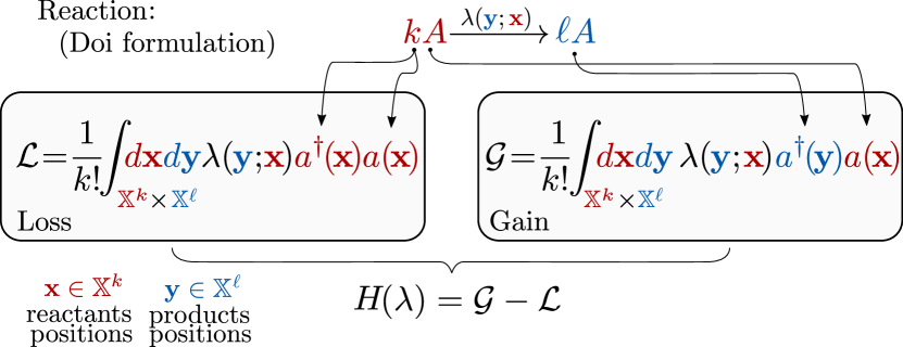
Figure 5: Diagram illustrating how to construct the generator for a system with a general one species reaction with rate function $\lambda(\mathbf{y};\mathbf{x})$ for the Doi formulation. This case takes into account the spatial dynamics in continuous space, and it is a special case of the basis-independent case presented in Fig. 4.

V.3 Representation in terms of scalar probability densities

In some cases, it might be helpful to work with an alternative representation of the CDME. For instance, some physical chemists and applied mathematicians might not be familiar with the bra-ket notation, so we could write the CDME directly in terms of the densities $\rho_{m}(x^{(n)})$. From Eq. 217, we know these densities are $\rho_{n}(x^{(n)})=\langle x^{n}|\rho\rangle$. We apply this to the example from Section V.2 (reaction $kA\rightarrow\ell A$). We begin by multiplying the CDME $\partial_{t}|\rho\rangle=H|\rho\rangle$ by $\langle x^{n}|$ on the left,

$$\partial_{t}\rho_{n}(x^{(n)})=\langle x^{n}|H|\rho\rangle.$$ (236)

The time derivative on the left hand side commutes, so it can be written directly in terms of the density. The right hand side can be written in terms of $\rho_{n}(x^{(n)})$ as well, but it requires careful consideration. We substitute the copy number representation of $|\rho\rangle$ (Eq. 216),

$$\langle x^{n}|H|\rho\rangle=\sum_{m\geq 0}\int_{\mathbb{X}^{m}}\ \langle x^{n}|H|y^{m}\rangle\ \rho_{m}(y^{(m)})dy^{(m)},$$ (237)

so we only need to calculate the term $\langle x^{n}|H|y^{m}\rangle$. We can further split this term into the diffusion and reaction components components: $\langle x^{n}|H|y^{m}\rangle=\langle x^{n}|H_{0}(D)|y^{m}\rangle+\langle x^{n}|H(\lambda)|y^{m}\rangle$. We begin with the diffusion part, the quantity $\langle x^{n}|H_{0}(D)|y^{m}\rangle$ can be simplified by using the expansion of the diffusion coefficient (Eq. 229) and of the bras and kets (Eq. 213),

$$\langle x^{n}|H_{0}(D)|y^{m}\rangle$$ (238)

$$=\frac{1}{n!}\int_{\mathbb{X}}dz\ \langle 0|a(x^{(n)})\ a^{\dagger}(z)\,D\nabla_{z}^{2}\,a(z)\ a^{\dagger}(y^{(m)})|0\rangle$$

$$=\frac{nm}{n!}\int_{\mathbb{X}}dz\delta_{z}(x_{1})D\nabla_{z}^{2}\delta_{z}(y_{1})\ \langle 0|a(x^{(n)}_{\setminus\{1\}})a^{\dagger}(y^{(m)}_{\setminus\{1\}})|0\rangle$$

$$=m\int_{\mathbb{X}}dz\ \delta_{z}(x_{1})\,D\nabla_{z}^{2}\,\delta_{z}(y_{1})\delta_{n,m}\delta(y^{(n)}_{\setminus\{1\}}-x^{(n)}_{\setminus\{1\}})$$

$$=\delta_{n,m}m\,D\nabla_{x_{1}}^{2}\,\delta(y^{(n)}-x^{(n)})$$

where we used the compact notation for Dirac deltas: $\delta_{y}(x)\equiv\delta(x-y)$. To obtain this result, we used Eqs. 224 and 225 to simplify the equations in the third line and Eqs. 227 and 228 to obtain the fourth line. The vacuum properties Eq. 212 were used to eliminate all the additional terms. Incorporating this into the form of Eq. 237, we obtain

$$\langle x^{n}|H_{0}(D)|\rho\rangle =nD\nabla_{x_{1}}^{2}\rho_{n}(x^{(n)})$$ (239)

$$=\sum_{i=1}^{n}D\nabla_{x_{i}}^{2}\rho_{n}(x^{(n)}),$$

where in the last line we used the symmetry of the density to express it in a more familiar form as the sum over the diffusion applied to each particle. Similar expressions are obtained analogously for the reaction operator $H(\lambda)=\mathcal{G}-\mathcal{L}$. We first calculate

$$\langle x^{n}|\ \mathcal{G}\ |y^{m}\rangle =$$ (240)

$$\delta_{n,m-k+\ell} \frac{m!\ \ell!}{n!\ k!}\sum_{\bm{\nu}\in S_{n}^{(\ell)}}\lambda\left(x^{(n)}_{\bm{\nu}};y^{(m)}_{[k]}\right)\delta\left(y^{(m)}_{\setminus[k]}-x^{(n)}_{\setminus\{\bm{\nu}\}}\right),$$

and

$$\langle x^{n}|\ \mathcal{L}\ |y^{m}\rangle =$$ (241)

$$\delta_{n,m} \sum_{\bm{\nu}\in S_{n}^{(k)}}\int_{\mathbb{X}^{\ell}}\lambda\left(\mathbf{z};x^{(n)}_{\bm{\nu}}\right)\delta(y^{(n)}-x^{(n)})\mathbf{dz}.$$

with $[k]=1,\dots,k$ and the ordered sums follows Eq. 226. Based on Eq. 237, we use these expressions to obtain the final form

$$\langle x^{n}|\ \mathcal{G}\ |\rho\rangle=\frac{(n-\Delta)!\ \ell!}{n!\ k!}$$ (242)

$$\qquad\times\int_{\mathbb{X}^{k}}\sum_{\bm{\nu}\in S_{n}^{(\ell)}}\lambda\left(x^{(n)}_{\bm{\nu}};\mathbf{z}\right)\rho_{n-\Delta}(\mathbf{z},x^{(n)}_{\setminus\{\bm{\nu}\}})\,\mathbf{dz}$$

$$={n\choose\ell}^{-1}{n-\Delta\choose k}$$ (243)

$$\qquad\times\sum_{\bm{\nu}\in S_{n}^{(\ell)}}\int_{\mathbb{X}^{k}}\lambda\left(x^{(n)}_{\bm{\nu}};\mathbf{z}\right)\rho_{n-\Delta}\left(\mathbf{z},x^{(n)}_{\setminus\{\bm{\nu}\}}\right)\,\mathbf{dz},$$

with $\Delta:=\ell-k$, and similarly for the loss

$$\langle x^{n}|\ \mathcal{L}\ |\rho\rangle =\sum_{\bm{\nu}\in S_{n}^{(k)}}\rho_{n}(x^{n})\int_{\mathbb{X}^{\ell}}\lambda\left(\mathbf{z};x^{(n)}_{\bm{\nu}}\right)\mathbf{dz}.$$ (244)

Now all the terms in Eq. 236 are expressed uniquely in terms of the densities:

$$\partial_{t}\rho_{n}(x^{(n)})=\langle x^{n}|H_{0}(D)|\rho\rangle+\langle x^{n}|\mathcal{G}|\rho\rangle-\langle x^{n}|\mathcal{L}|\rho\rangle.$$ (245)

The results obtained are consistent with the expected results previously obtained in [182]. A similar calculation can also be performed using the basis-independent representation.

V.4 Fluxes and many-particle propensities

It is often useful for practitioners to write the CDME in terms of probability fluxes, for instance when studying nonequilibrium processes and their driving forces [175, 173, 19] or more generally stochastic thermodynamics [110, 35]. For simplicity, we present this formulation based on the Doi formulation from Section V.1, but the general basis-independent case from Section IV follows the same logic.

We again assume a system with one reaction given by the general one species chemical reaction ($kA\rightarrow\ell A$ with $\Delta:=\ell-k$) following Section V.2, and we define two fluxes: the influx $J^{+}_{n}$ from any particle state into the current state with $n-$particles, and the outflux $J^{-}_{n}$ from the current $n-$particle state to any other state. The influx operator applied to the density ket $|\rho\rangle$ should yield the probability flux into state $|x^{n}\rangle$ from $\rho_{n}$ due to the corresponding reaction. We can calculate this expression explicitly from the gain operator as

$$\begin{split}J^{+}_{n}(x^{(n)})&=\langle x^{n}|\ \mathcal{G}\ |\rho\rangle\\ &=\sum_{m\geq 0}\int_{\mathbb{X}^{m}}\langle x^{n}|\ \mathcal{G}\ |y^{m}\rangle\langle y^{m}|\rho\rangle dy^{(m)}\\ &=\sum_{m\geq 0}\int_{\mathbb{X}^{m}}\langle x^{n}|\ \mathcal{G}\ |y^{m}\rangle\rho_{m}(y^{(m)})dy^{(m)},\\ &=\int_{\mathbb{X}^{n-\Delta}}\langle x^{n}|\ \mathcal{G}\ |y^{n-\Delta}\rangle\rho_{n-\Delta}(y^{(n-\Delta)})dy^{(n-\Delta)},\end{split}$$ (246)

since it is only non-zero for $m=n-\Delta$. Similarly for the outflux, we use the loss operator

$$\begin{split}J^{-}_{n}(x^{(n)})&=\langle x^{n}|\ \mathcal{L}\ |\rho\rangle\\ &=\sum_{m\geq 0}\int_{\mathbb{X}^{m}}\langle x^{n}|\ \mathcal{L}\ |y^{m}\rangle\rho_{m}(y^{(m)})dy^{(m)},\\ &=\int_{\mathbb{X}^{n}}\langle x^{n}|\ \mathcal{L}\ |y^{n}\rangle\rho_{n}(y^{(n)})dy^{(n)},\end{split}$$ (247)

since it yields $0$ for $m\neq n$. Thus, analogous to Eq. 245, we can write the CDME as

$$\partial_{t}\rho_{n}(x^{(n)})=D\nabla^{2}\rho_{n}(x^{(n)})+J^{+}_{n}(x^{(n)})-J^{-}_{n}(x^{(n)}).$$ (248)

Note we already computed these expressions explicitly in Section V.3. We can further rewrite the equations in terms of the many-particle propensities $\Lambda_{n}$ introduced in [182],

$$\Lambda_{n-\Delta}\left(x^{(n)};y^{(n-\Delta)}\right):=\langle x^{n}|\ \mathcal{G}\ |y^{n-\Delta}\rangle,$$ (249)

which denotes the transfer of probability density from the $n-\Delta$ to the $n$ state per unit time for the corresponding reaction. The influx (gain) and outflux (loss) are expressed as

$$J^{+}_{n}(x^{(n)}) =\int_{\mathbb{X}^{n-\Delta}}\Lambda_{n-\Delta}\left(x^{(n)};\bm{z}\right)\rho_{n-\Delta}(\bm{z})d\bm{z}$$ (250)

$$J^{-}_{n}(x^{(n)}) =\rho_{n}(x^{(n)})\int_{\mathbb{X}^{n+\Delta}}\Lambda_{n}\left(\bm{z};x^{(n)}\right)d\bm{z},$$ (251)

yielding an alternative way to write the CDME, which perhaps is more intuitive for some applications. The first equation is exactly the same than Eq. 246. Although not as trivial, the second one is analogously equal to Eq. 247, which can be proven by direct substitution of Eq. 249 and Eqs. 241 and 240.

For an arbitrary system of $R$ reactions involving one species, one can write the total fluxes in terms of the sums of losses and gain over the reactions

$$J^{+}_{n}(x^{(n)})=\sum_{r=1}^{R}\langle x^{n}|\mathcal{G}^{(r)}|\rho\rangle\ ,\quad J^{-}_{n}(x^{(n)})=\sum_{r=1}^{R}\langle x^{n}|\mathcal{L}^{(r)}|\rho\rangle.$$ (252)

Alternatively, one can also write them in terms of the propensity functions $\Lambda_{m}\left(x^{(n)};y^{(m)}\right):=\sum_{r=1}^{R}\langle x^{n}|\ \mathcal{G}^{(r)}\ |y^{m}\rangle,$ as

$$J^{+}_{n}(x^{(n)}) =\sum_{\begin{subarray}{c}m\geq 0\\ m\neq n\end{subarray}}\int_{\mathbb{X}^{m}}\Lambda_{m}\left(x^{(n)};\bm{z}\right)\rho_{m}(\bm{z})d\bm{z}$$ (253)

$$J^{-}_{n}(x^{(n)}) =\sum_{\begin{subarray}{c}m\geq 0\\ m\neq n\end{subarray}}\rho_{n}(x^{(n)})\int_{\mathbb{X}^{m}}\Lambda_{n}\left(\bm{z};x^{(n)}\right)d\bm{z},$$ (254)

The general equation with multiple species will have the same form, but the notation needs to keep track of the species numbers and positions for each species.

V.5 Stochastic concentrations

The family of densities (Eq. 139) yields the probability distribution of finding $n$ particles at locations $x^{(n)}$ for all $n$. On the other hand, suppose we want to know the distribution of finding $n$ particles in some delimited region in space at time $t$, or more precisely the stochastic concentration of particles at some point $(x,t)$ in space and time . For this purpose, we introduce the density/concentration operator

$$\mathcal{C}_{x}=a^{\dagger}(x)a(x),$$ (255)

when applying it to $|\rho\rangle$ from Eq. 216, it yields the stochastic concentration $|C(x)\rangle$

$$\begin{split}|C(x)\rangle&=\mathcal{C}_{x}|\rho\rangle\\ &=a^{\dagger}(x)a(x)\sum_{m\geq 0}\int_{\mathbb{X}^{m}}dz^{(m)}\rho_{m}(z^{(m)})|z^{m}\rangle\\ &=\sum_{m\geq 0}\int_{\mathbb{X}^{m}}dz^{(m)}\rho_{m}(z^{(m)})a^{\dagger}(x)a(x)a^{\dagger}(z^{m})|0\rangle\\ &=\sum_{m\geq 1}m\int_{\mathbb{X}^{m-1}}dz^{(m-1)}\rho_{m}(x,z^{(m-1)})|z^{m-1}\rangle,\end{split}$$ (256)

where we used Eq. 223 to simplify. This corresponds to the concentration as one recovers the same expression when calculating the number of molecules in a region divided by the volume and taking the limit as the volume goes to zero [179]. We can also apply it to the diffusion generator, $\mathcal{C}_{x}H_{0}(D)$,

$$\begin{split}\mathcal{C}_{x}H_{0}(D)&=a^{\dagger}(x)a(x)\int_{\mathbb{X}}dz\ a^{\dagger}(z)\,D\nabla_{z}^{2}\,a(z)\\ &\quad=\int_{\mathbb{X}}dz\ \Big{(}\ a^{\dagger}(z)\,D\nabla_{z}^{2}\,a(z)a^{\dagger}(x)a(x)\\ &\qquad\qquad+a^{\dagger}(x)\nabla_{x}^{2}a(x)-\nabla_{x}^{2}(a^{\dagger}(x))a(x)\ \Big{)}\\ &\quad=H_{0}(D)\mathcal{C}_{x}+a^{\dagger}(x)\nabla_{x}^{2}a(x)-\nabla_{x}^{2}(a^{\dagger}(x))a(x),\end{split}$$ (257)

which is proven with the commutation relations Eq. 211 and by integration by parts. Note that to commute with the differential operator, we need to write the diffusion operator in the form of Eq. 220 and apply the Dirac delta integrals in the distributional sense after commuting with the creation and annihilation operators. This yields the following commutation relation: $[\mathcal{C}_{x},H_{0}(D)]=a^{\dagger}(x)\nabla_{x}^{2}a(x)-\nabla_{x}^{2}(a^{\dagger}(x))a(x)$.

One can apply the density operator to an arbitrary CDME $\partial_{t}|\rho\rangle=H|\rho\rangle$ to yield the equation for the stochastic concentrations

$$\begin{split}\partial_{t}|C(x)\rangle&=\mathcal{C}_{x}H|\rho\rangle\\ &=\left[\mathcal{C}_{x},H\right]|\rho\rangle+H\mathcal{C}_{x}|\rho\rangle\\ &=\left[\mathcal{C}_{x},H\right]|\rho\rangle+H|C(x)\rangle,\end{split}$$ (258)

written in terms of the commutator. As we observed for the diffusion generator, the term $\left[\mathcal{C}_{x},H\right]|\rho\rangle$ is in general not trivial. In specific cases, especially when taking the expectation value or mean-field approximation, the calculations simplify, as in the specific example covered below in Section V.6. In other cases, this term might be helpful to calculate fluctuations around the mean-field since it is related to higher-order moments.

Note that one can define the particle number operator similarly as integrals of the density/concentration operator,

$$\mathcal{N}=\int_{\mathbb{X}}dx\ a^{\dagger}(x)a(x),\quad\mathcal{N}_{\Omega}=\int_{\Omega}dx\ a^{\dagger}(x)a(x),$$ (259)

such that $\mathcal{N}|\rho\rangle=N|\rho\rangle$ yields the stochastic number of particles in the whole domain $\mathbb{X}$ and $\mathcal{N}_{\Omega}|\rho\rangle$ the same but in a subdomain $\Omega$, analogous to Eq. 155. If we repeat the calculations from Eq. 257 for the particle number operator, the commutator is zero $\left[\mathcal{N},H_{0}(D)\right]=0$, which means the diffusion process alone does not change the total number of particles. Applying $\mathcal{N}$ to the CDME removes the spatial dependence and yields the chemical master equation from Section II.3. However, this is not necessarily trivial to calculate explicitly for systems with nonlinear reactions due to diffusion-influenced processes [69, 177].

V.6 Emergence of macroscopic reaction-diffusion equations

In the same spirit as in Section II.4, we want to obtain the mean-field equations with space dependence, see Fig. 1. To do this, we first show some of the properties of the flat state $\langle 1|$ in the spatially dependent setting. The flat state is simply the dual coherent state from Eq. 219 with $z=1$. Analogous to Eq. 19, the first property is $\langle 1|=\langle 1|a^{\dagger}(x)$. Next, we apply the flat state to the density from Eq. 216

$$\langle 1|\rho\rangle=1,$$

which we verify by simply expanding $\langle 1|$ and $|\rho\rangle$, using the orthonormal property (Eq. 215) and that the distribution is normalized. In fact, applying $\langle 1|$ corresponds to summing over the whole phase space [68]

$$\langle 1|=\sum_{m\geq 0}\int_{\mathbb{X}^{m}}dx^{(m)}\cdots.$$ (260)

Similarly one can show that $\langle 1|y^{m}\rangle=1$ since $\langle 1|y^{m}\rangle=\langle 1|a^{\dagger}(y^{(m)})|0\rangle=\langle 1|0\rangle=1$.

As we are interested in the mean-field evolution of specific observables, we first need to apply an operator such as the density operator $\mathcal{C}_{x}=a^{\dagger}(x)a(x)$, and then take the expectation. Thus we are interested in the action of $\langle 1|\mathcal{C}_{x}$. Applying this to the density we obtain

$$\langle 1|\mathcal{C}_{x}|\rho\rangle =\langle 1|\sum_{m\geq 1}m\int_{\mathbb{X}^{m-1}}dz^{(m-1)}\rho_{m}(x,z^{(m-1)})|z^{m-1}\rangle$$

$$=\sum_{m\geq 1}m\int_{\mathbb{X}^{m-1}}\mathbf{dz}\,\rho_{m}(x,\mathbf{z}),$$ (261)

where we used Eq. 256 and the properties of the flat state derived above. This equation corresponds exactly to the equation for the expected value of the concentration at a point $x$ derived in [179], showing consistency between the different approaches. This equation hints to two possible pathways to calculate the expectation values for the concentrations: the left hand side using the bra-ket notation with creation and annihilation operators and the right hand side using the integrals. We follow the first one and apply it to the master equation for a diffusion process $\partial_{t}|\rho\rangle=H_{0}(D)|\rho\rangle$

$$\langle 1|\mathcal{C}_{x}\partial_{t}|\rho\rangle=\langle 1|\mathcal{C}_{x}H_{0}(D)|\rho\rangle,$$ (262)

which simplifies to

$$\partial_{t}c(x)=\langle 1|\mathcal{C}_{x}H_{0}(D)|\rho\rangle$$ (263)

with $c(x)=\mathrm{E}[C(x)]=\langle 1|\mathcal{C}_{x}|\rho\rangle$ the expected concentration at $x$. We can simplify further the right hand side

$$\begin{split}&\langle 1|\mathcal{C}_{x}H_{0}(D)|\rho\rangle=\langle 1|a^{\dagger}(x)a(x)\int_{\mathbb{X}}dz\ a^{\dagger}(z)D\nabla^{2}a(z)|\rho\rangle\\ &\quad=D\nabla_{x}^{2}c(x)+\langle 1|H_{0}(D)a(x)|\rho\rangle\\ &\quad=D\nabla_{x}^{2}c(x),\end{split}$$ (264)

where we used the commutation relations from Eq. 211, and we used the properties of the flat state: $\langle 1|a^{\dagger}(x)=\langle 1|$ and $\langle 1|H=0$, where $H$ is any probability conserving infinitesimal generator, as shown in Eq. 27. This recovers the macroscopic diffusion equation $\partial_{t}c(x)=D\nabla^{2}c(x)$. To cover more interesting cases, now we explore reactions in spatially-dependent domains.

To showcase the power of the method, we focus directly on a nonlinear/bimolecular reaction-diffusion system: mutual annihilation $A+A\rightarrow\emptyset$ with rate function $\lambda(z_{1},z_{2})$, where $z_{1}$ and $z_{2}$ are the positions of the two reactants. We will often simplify notation to $\bm{z}=(z_{1},z_{2})$. Following the formulas for the loss and gain for a general one-species reaction from Eq. 234 and Eq. 235, by using $k=2$ and $l=0$, we obtain the loss and gain generators for the mutual annihilation reaction

$$\begin{aligned} \mathcal{L}&=\frac{1}{2}\int_{\mathbb{X}^{2}}d\bm{z}a^{\dagger}(\bm{z})\lambda(\bm{z})a(\bm{z}),\\ \mathcal{G}&=\frac{1}{2}\int_{\mathbb{X}^{2}}d\bm{z}\lambda(\bm{z})a(\bm{z}).\end{aligned}$$ (265)

The probability conserving infinitesimal generator for the mutual annihilation reaction is $H_{m}(\lambda)=\mathcal{G}-\mathcal{L}$. Analogous to the diffusion case, we obtain the mean-field equations by calculating

$$\begin{split}\langle 1|\mathcal{C}_{x}H_{m}(\lambda)|\rho\rangle&=\langle 1|a^{\dagger}(x)a(x)(\mathcal{G}-\mathcal{L})|\rho\rangle\\ &=\langle 1|a(x)\mathcal{G}|\rho\rangle-\langle 1|a(x)\mathcal{L}|\rho\rangle\end{split}$$ (266)

Because the operators commute (Eq. 211), the first term is simply

$$\begin{split}\langle 1|a(x)\mathcal{G}|\rho\rangle&=\langle 1|a(x)\frac{1}{2}\int_{\mathbb{X}^{2}}d\bm{z}\lambda(\bm{z})a(\bm{z})|\rho\rangle\\ &=\langle 1|\frac{1}{2}\int_{\mathbb{X}^{2}}d\bm{z}\lambda(\bm{z})a(\bm{z})a(x)|\rho\rangle.\end{split}$$ (267)

Similarly, the second term is computed with the same commutation relations, with the relations from Eq. 223 and with the properties of the flat state,

$$\langle 1|a(x)\mathcal{L}|\rho\rangle=\langle 1|\frac{1}{2}\int_{\mathbb{X}^{2}}d\bm{z}\ a(x)a^{\dagger}(\bm{z})\lambda(\bm{z})a(\bm{z})|\rho\rangle$$

$$\quad=\langle 1|\int_{\mathbb{X}^{2}}d\bm{z}\ \lambda(\bm{z})\delta(x-z_{1})a^{\dagger}(z_{2})a(\bm{z})|\rho\rangle$$

$$\qquad+\langle 1|\frac{1}{2}\int_{\mathbb{X}^{2}}d\bm{z}\lambda(\bm{z})a(\bm{z})a(x)|\rho\rangle,$$ (268)

with $\bm{z}=(z_{1},z_{2})$. Gathering the loss and gain terms, two terms cancel and only one integral survives

$$\langle 1|\mathcal{C}_{x}H_{m}(\lambda)|\rho\rangle =\langle 1|\int_{\mathbb{X}^{2}}d\bm{z}\lambda(\bm{z})\delta(x-z_{1})a^{\dagger}(z_{2})a(\bm{z})|\rho\rangle$$

$$=\langle 1|\int_{\mathbb{X}}dz\ \lambda(x,z)a(x)a(z)|\rho\rangle$$

$$=\int_{\mathbb{X}}dz\ \lambda(x,z)\ \langle 1|a(x)a(z)|\rho\rangle.$$ (269)

We recognize that the term $\langle 1|a(x)a(z)|\rho\rangle$ corresponds to the expectation of the second-order particle number/density operator, i.e. $\mathrm{E}[C(z)C(x)]=\langle 1|\mathcal{C}_{z}\mathcal{C}_{x}|\rho\rangle$. In general $\mathrm{E}[C(z)C(x)]=\mathrm{E}[C(z)]\mathrm{E}[C(x)]+\mathrm{Cov}(C(z),C(x))$, thus

$$\langle 1|\mathcal{C}_{x}H_{m}(\lambda)|\rho\rangle =\int_{\mathbb{X}}\lambda(x,z)\ c(x)c(z)dz$$ (270)

$$\qquad+\int_{\mathbb{X}}\ \lambda(x,z)\mathrm{Cov}(C(z),C(x))dz.$$

To obtain a closed equation, we need to choose the form of the rate function $\lambda(x,z)$. We choose a simple indicator function $\lambda(x,z)=\kappa\mathbb{1}_{|x-z|\leq\sigma}$, which corresponds with particle reacting with constant rate $\kappa$ if their relative distance is less or equal to $\sigma$ [69]. Moreover, if the number of particles is large enough, the covariance is negligible in comparison with the product of the means due to the law of large numbers [5, 135]. Thus, assuming large copy numbers, then $\mathrm{Cov}(C(z),C(x))\rightarrow 0$ [177], and we are left with

$$\begin{split}\langle 1|\mathcal{C}_{x}H_{m}(\lambda)|\rho\rangle&\approx\int_{\mathbb{X}}\kappa\mathbb{1}_{|x-z|\leq\sigma}\ c(x)c(z)\ dz\\ &\approx\kappa\int_{\mathbb{X}}\mathbb{1}_{|x-z|\leq\sigma}\ c(x)^{2}\ dz\\ &=\kappa\frac{4\pi}{3}\sigma^{3}c(x)^{2},\\ \end{split}$$ (271)

where we further assumed the region sigma is small enough, so we can approximate $c(z)$ by its center value $c(x)$ in this region. Thus the emerging reaction-diffusion master equation for the mutual annihilation reaction is

$$\partial_{t}c(x)=D\nabla^{2}c(x)-rc(x)^{2}\quad\text{with}\quad r=\kappa\frac{4\pi}{3}\sigma^{3},$$ (272)

where $r$ is the macroscopic rate given in terms of the microscopic parameters $\sigma$ and $\kappa$. This result is consistent with previous results based on the corresponding convergent RDME [135] and also more recently on the CDME using standard methods [177] and proven rigorously in [115]. This derivation can be generalized by taking into account the covariance, or base the results on more complex rate functions, yielding novel meso- and macroscopic equations.

VI Concluding remarks and future scope

We presented a unified and structured general framework for field theory representations of reaction-diffusion processes. Throughout this process, we reviewed a large body of previous work and placed this within the general framework (Fig. 1). In particular, from the basis-independent representation with continuous spatial resolution, we obtained various other field theory representations as special and/or limiting cases. We further exposed the relationships with well-known chemical physics models, and we showed how to obtain numerical discretizations, as well as meso- and/or macroscopic emerging models using field theory techniques. In addition, we provided an overview of the path-integral representations, which combined with the Galerkin discretization, yields an approach to obtain discretized meso/macroscopic models directly from the formulation at the particle level. To spark the interest of the reader, we delved briefly into some advanced topics of interest as large deviation theory, perturbation theory, renormalization group methods, and master equations for stochastic concentrations.

The framework is presented in the context of reaction-diffusion, partly to keep the presentation simple and also due to the extensive applicability of reaction-diffusion processes. However, with a few modifications, one can extend the framework to a larger class of systems, while preserving the structure presented in Fig. 1. For instance, it is possible to take inertia into account by incorporating velocities into the dynamics. The diffusion terms would then model the Newtonian mechanics in the form of Liouville equations. If noise in the form of a thermostat is included, it transforms into Langevin dynamics whose probabilistic description is given by the Klein-Kramers equation [181, 68, 213]. On the other hand, the reaction part is not limited to model reactions; for instance, it could also model the addition or removal of particle due to interactions with a reservoir. We can thus extend the framework for these and other systems, as already partly explored for specific cases [181, 177, 69, 95]. From a dynamical systems point of view, we can take it one step beyond. We can, in principle, apply it to any Markovian dynamical system—deterministic or stochastic—with variable particle numbers. Thus, this is a very general approach to handle classical dynamical systems with varying particle numbers and could be expanded to non-Markovian dynamics.

In the context of general dynamical systems, the application scope broadens considerably. The methods presented comprise a unified toolkit to operate on the probabilistic dynamics of particle or agent-based models with varying numbers: one can perform calculations, discretizations and derive emergent models at multiple scales without handling the combinatorics explicitly. Each of the different representations, such as the basis-independent, the Doi formulation or the Galerkin discretization, prove to be useful in different contexts and aid in establishing connections between the models at different scales. Using these methods and representations, it is possible to create mathematical bridges between particle or agent-based models of complex systems and their meso- and macroscopic descriptions. These bridges constitute the scaffolding to construct consistent numerical methods of complex systems across scales, as already shown for reaction-diffusion systems in specific settings [77, 126, 135, 178, 177, 200, 225].

In particular, in the context of emerging models, we developed a consistent methodology to obtain meso- and macroscopic models using field theory techniques. The coarser descriptions emerge from specific limits or mean-field approximation of the finer levels. For instance, using the stochastic concentration description from Section V.5, we can take the expectations by applying the flat state on the left, yielding a macroscopic PDE. Moreover, it is also possible to construct a stochastic PDE based on the stochastic concentration description itself. For instance, one could calculate the equations for the second and/or higher moments and characterize the features of the space-time noise term. Research on stochastic PDEs has been increasing considerably in the last decades [100, 101, 165], specially in the context of multiscale modeling [1, 103, 15, 104, 219], and it is a promising field of application for the techniques presented in this work.

There are several relevant extensions of the techniques presented here in connection with other fields. Of particular interest is in the context of open driven (stochastic) quantum systems [199] and their thermodynamics [56, 134], which are often modeled with master equations of the Lindblad type [143]. There is on-going research on the correct form of this equation to model material exchange with reservoirs [56, 60], and it might be possible to reformulate the framework presented here in this setting. Another interesting extension is in the direction of stochastic thermodynamics [172, 35, 230], which has not been fully established in the context of reaction-diffusion processes due to their inherent complexity. The formulations presented here provide an accessible framework for this development. In connection with mathematics, the groundbreaking theory of regularity structures [101] provides an algebraic framework that gives a mathematically rigorous meaning to many stochastic PDEs. This theory was partly inspired by the mathematical analysis of field theories, so it is of interest to explore its connections with the work presented here. This could make the results of the theory accessible and applicable to a broader audience. Additional extensions consist of incorporating the Kolmogorov backward equations in the general setting by following [218], as well as making the link between the generic field theory and large deviation theory more robust, see for instance [201, 10, 138, 33].

Taking all this into consideration, we envision applications to multi-scale modeling and simulation of complex systems in a diverse range of domains. Especially interesting are those which cross the boundaries of existing disciplines, such as the use of stochastic predator-prey systems to model the onset of turbulence [198], or the renormalization group analysis of swarms of active particles [53]. We also foresee possible applications in enzyme kinetics and cascades [137], cellular and molecular biology [76, 31], tumor migration models [63], bacterial dynamics [209], stochastic population dynamics [10], gene expression models [32], actin filament and microtubule growth [164] and neurological applications from molecular transport and firing in neurons, to cognitive phenonema such as decision making [54]. Ultimately, the methods described here could also be useful in multiscale modeling of socio-economical phenomena such as segregation [197], polarization, opinion and voter dynamics [104, 183] and economic inequality. With such a great potential for diverse applications, we hope that this work helps to connect communities from different disciplines working on mathematically similar systems, as it demonstrates how existing applications in diverse fields are connected in a single unifying formalism.

References

- Abdulle and Pavliotis [2012] Abdulle, Assyr, and Grigorios A Pavliotis (2012), “Numerical methods for stochastic partial differential equations with multiple scales,” Journal of Computational Physics 231 (6), 2482–2497.
- Abrikosov et al. [1975] Abrikosov, AA, L.P. Gorkov, and I.E. Dzyaloshinski (1975), Methods of quantum field theory in statistical physics, Dover Books on Physics (Dover Publications, Mineola, NY).
- Agazzi et al. [2018] Agazzi, Andrea, Amir Dembo, and Jean-Pierre Eckmann (2018), “Large deviations theory for markov jump models of chemical reaction networks,” The Annals of Applied Probability 28 (3), 1821–1855.
- Anderson et al. [2010] Anderson, David F, Gheorghe Craciun, and Thomas G Kurtz (2010), “Product-form stationary distributions for deficiency zero chemical reaction networks,” Bulletin of mathematical biology 72, 1947–1970.
- Anderson and Kurtz [2015] Anderson, David F, and Thomas G Kurtz (2015), Stochastic analysis of biochemical systems, Vol. 674 (Springer).
- Andreanov et al. [2006] Andreanov, Alexei, Giulio Biroli, Jean-Philippe Bouchaud, and Alexandre Lefevre (2006), “Field theories and exact stochastic equations for interacting particle systems,” Physical Review E 74 (3), 030101.
- Antal and Schütz [2000] Antal, T, and G. M. Schütz (2000), “Asymmetric exclusion process with next-nearest-neighbor interaction: Some comments on traffic flow and a nonequilibrium reentrance transition,” Physical Review E 62 (1), 83.
- Araújo et al. [2020] Araújo, HA, MO Lukin, MGE da Luz, GM Viswanathan, FAN Santos, and EP Raposo (2020), “Revisiting lévy flights on bounded domains: a fock space approach,” Journal of Statistical Mechanics: Theory and Experiment 2020 (8), 083202.
- Armas et al. [2023] Armas, Jay, Wout Merbis, Janusz Meylahn, Soroush Rafiee Rad, and Mauricio J. del Razo (2023), “Risk aversion promotes cooperation,” 10.48550/ARXIV.2306.05971.
- Assaf and Meerson [2017] Assaf, Michael, and Baruch Meerson (2017), “WKB theory of large deviations in stochastic populations,” Journal of Physics A: Mathematical and Theoretical 50 (26), 263001.
- Baez and Biamonte [2017] Baez, John, and Jacob D Biamonte (2017), Quantum Techniques in Stochastic Mechanics (WORLD SCIENTIFIC).
- Baez [2018] Baez, John C (2018), “Quantum techniques for reaction networks,” Advances in Mathematical Physics 2018 (1), 7676309.
- Baez and Fong [2013] Baez, John C, and Brendan Fong (2013), “A Noether theorem for Markov processes,” Journal of Mathematical Physics 54 (1).
- Baez and Fong [2015] Baez, John C, and Brendan Fong (2015), “Quantum techniques for studying equilibrium in reaction networks,” Journal of Complex Networks 3 (1), 22–34.
- Baish and Vollmayr-Lee [2024] Baish, Andrew J, and Benjamin P Vollmayr-Lee (2024), “Fock space and field theoretic description of nonequilibrium work relations,” arXiv preprint arXiv:2405.02552 .
- Baras and Mansour [1996] Baras, Florence, and M Malek Mansour (1996), “Reaction-diffusion master equation: A comparison with microscopic simulations,” Physical Review E 54 (6), 6139.
- Bartmanski and Baker [2020] Bartmanski, Bartosz J, and Ruth E Baker (2020), “StoSpa2: A C++ software package for stochastic simulations of spatially extended systems,” Journal of Open Source Software 5 (50).
- Bausch et al. [1976] Bausch, R, Hans-Karl Janssen, and Ho Wagner (1976), “Renormalized field theory of critical dynamics,” Zeitschrift fur Physik B Condensed Matter 24 (1), 113–127.
- Beard and Qian [2007] Beard, Daniel A, and Hong Qian (2007), “Relationship between thermodynamic driving force and one-way fluxes in reversible processes,” PloS one 2 (1), e144.
- Beard and Qian [2008] Beard, Daniel A, and Hong Qian (2008), Chemical biophysics: quantitative analysis of cellular systems, Vol. 126 (Cambridge University Press Cambridge).
- Behr et al. [2016] Behr, Nicolas, Vincent Danos, and Ilias Garnier (2016), “Stochastic mechanics of graph rewriting,” in Proceedings of the 31st Annual ACM/IEEE Symposium on Logic in Computer Science, pp. 46–55.
- Behr et al. [2017] Behr, Nicolas, Gerard HE Duchamp, and Karol A Penson (2017), “Combinatorics of chemical reaction systems,” arXiv preprint arXiv:1712.06575 .
- Bell et al. [1994] Bell, John, Marsha Berger, Jeff Saltzman, and Mike Welcome (1994), “Three-dimensional adaptive mesh refinement for hyperbolic conservation laws,” SIAM Journal on Scientific Computing 15 (1), 127–138.
- Benitez et al. [2016] Benitez, Federico, Charlie Duclut, Hugues Chaté, Bertrand Delamotte, Ivan Dornic, and Miguel A Muñoz (2016), “Langevin equations for reaction-diffusion processes,” Physical Review Letters 117 (10), 100601.
- Bettelheim et al. [2001] Bettelheim, Eldad, Oded Agam, and Nadav M Shnerb (2001), ““quantum phase transitions” in classical nonequilibrium processes,” Physica E: Low-dimensional Systems and Nanostructures 9 (3), 600–608.
- Bleher and Bleher [2024] Bleher, Johannes, and Michael Bleher (2024), “An algebraic framework for the modeling of limit order books,” arXiv preprint arXiv:2406.04969 .
- Bleher et al. [2020] Bleher, Johannes, Michael Bleher, and Thomas Dimpfl (2020), “From orders to prices: A stochastic description of the limit order book to forecast intraday returns,” arXiv preprint arXiv:2004.11953 .
- Bothe and Pruessner [2021] Bothe, Marius, and Gunnar Pruessner (2021), “Doi-peliti field theory of free active ornstein-uhlenbeck particles,” Physical Review E 103 (6), 062105.
- Bramson and Lebowitz [1991] Bramson, Maury, and Joel L Lebowitz (1991), “Spatial structure in diffusion-limited two-particle reactions,” Journal of statistical physics 65, 941–951.
- Bressloff [2010] Bressloff, Paul C (2010), “Stochastic neural field theory and the system-size expansion,” SIAM Journal on Applied Mathematics 70 (5), 1488–1521.
- Bressloff [2014] Bressloff, Paul C (2014), Stochastic processes in cell biology, Vol. 41 (Springer).
- Bressloff [2017] Bressloff, Paul C (2017), “Stochastic switching in biology: from genotype to phenotype,” Journal of Physics A: Mathematical and Theoretical 50 (13), 133001.
- Bressloff [2021] Bressloff, Paul C (2021), “Coherent spin states and stochastic hybrid path integrals,” Journal of Statistical Mechanics: Theory and Experiment 2021 (4), 043207.
- Bressloff and Newby [2014] Bressloff, Paul C, and Jay M Newby (2014), “Path integrals and large deviations in stochastic hybrid systems,” Physical Review E 89 (4), 042701.
- Van den Broeck [2013] Van den Broeck, Christian (2013), “Stochastic thermodynamics: A brief introduction,” in Physics of Complex Colloids (IOS Press) pp. 155–193.
- Buice and Chow [2007] Buice, Michael A, and Carson C Chow (2007), “Correlations, fluctuations, and stability of a finite-size network of coupled oscillators,” Physical Review E—Statistical, Nonlinear, and Soft Matter Physics 76 (3), 031118.
- Buice and Chow [2013] Buice, Michael A, and Carson C Chow (2013), “Dynamic finite size effects in spiking neural networks,” PLoS computational biology 9 (1), e1002872.
- Buice and Cowan [2007] Buice, Michael A, and Jack D Cowan (2007), “Field-theoretic approach to fluctuation effects in neural networks,” Physical Review E 75 (5), 051919.
- Buice and Cowan [2009] Buice, Michael A, and Jack D Cowan (2009), “Statistical mechanics of the neocortex,” Progress in biophysics and molecular biology 99 (2-3), 53–86.
- Buice et al. [2010] Buice, Michael A, Jack D Cowan, and Carson C Chow (2010), “Systematic fluctuation expansion for neural network activity equations,” Neural computation 22 (2), 377–426.
- Burioni and Cassi [2005] Burioni, Raffaella, and Davide Cassi (2005), “Random walks on graphs: ideas, techniques and results,” Journal of Physics A: Mathematical and General 38 (8), R45.
- Butler and Goldenfeld [2009] Butler, Thomas, and Nigel Goldenfeld (2009), “Robust ecological pattern formation induced by demographic noise,” Physical Review E 80 (3), 030902.
- Butler and Goldenfeld [2011] Butler, Thomas, and Nigel Goldenfeld (2011), “Fluctuation-driven turing patterns,” Physical Review E 84 (1), 011112.
- Butler and Reynolds [2009] Butler, Thomas, and David Reynolds (2009), “Predator-prey quasicycles from a path-integral formalism,” Physical Review E 79 (3), 032901.
- Calisto and Tirapegui [1993] Calisto, H, and E Tirapegui (1993), “-expansion of van kampen through functional integrals,” Journal of statistical physics 71, 683–703.
- Cardy [1996] Cardy, John (1996), “Renormalisation group approach to reaction-diffusion problems,” arXiv preprint cond-mat/9607163 .
- Cardy [1999] Cardy, John (1999), “Field theory and nonequilibrium statistical mechanics,” Lectures Presented at the Troisieme Cycle de la Suisse Romande , 14.
- Cardy and Täuber [1996] Cardy, John, and Uwe C Täuber (1996), “Theory of branching and annihilating random walks,” Physical review letters 77 (23), 4780.
- Cardy and Grassberger [1985] Cardy, John L, and Peter Grassberger (1985), “Epidemic models and percolation,” Journal of Physics A: Mathematical and General 18 (6), L267.
- Cardy and Sugar [1980] Cardy, John L, and RL Sugar (1980), “Directed percolation and reggeon field theory,” Journal of Physics A: Mathematical and General 13 (12), L423.
- Cardy and Täuber [1998] Cardy, John L, and Uwe C Täuber (1998), “Field theory of branching and annihilating random walks,” Journal of statistical physics 90, 1–56.
- Castellano et al. [2009] Castellano, Claudio, Santo Fortunato, and Vittorio Loreto (2009), “Statistical physics of social dynamics,” Reviews of modern physics 81 (2), 591.
- Cavagna et al. [2023] Cavagna, Andrea, Luca Di Carlo, Irene Giardina, Tomás S Grigera, Stefania Melillo, Leonardo Parisi, Giulia Pisegna, and Mattia Scandolo (2023), “Natural swarms in 3.99 dimensions,” Nature Physics 19 (7), 1043–1049.
- Chow and Buice [2015] Chow, Carson C, and Michael A Buice (2015), “Path integral methods for stochastic differential equations,” The Journal of Mathematical Neuroscience (JMN) 5, 1–35.
- Dal Cengio et al. [2023] Dal Cengio, Sara, Vivien Lecomte, and Matteo Polettini (2023), “Geometry of nonequilibrium reaction networks,” Physical Review X 13 (2), 021040.
- Dann and Kosloff [2021] Dann, Roie, and Ronnie Kosloff (2021), “Quantum thermo-dynamical construction for driven open quantum systems,” Quantum 5, 590.
- Dawson et al. [1993] Dawson, Donald A, Bernard Maisonneuve, Joel Spencer, and Donald Dawson (1993), Measure-valued Markov processes (Springer).
- De Giuli and Scalliet [2022] De Giuli, Eric, and Camille Scalliet (2022), “Dynamical mean-field theory: from ecosystems to reaction networks,” Journal of Physics A: Mathematical and Theoretical 55 (47), 474002.
- Dechenaux et al. [2022] Dechenaux, Benjamin, Thomas Delcambre, and Eric Dumonteil (2022), “Percolation properties of the neutron population in nuclear reactors,” Physical Review E 106 (6), 064126.
- Delle Site and Djurdjevac [2024] Delle Site, Luigi, and Ana Djurdjevac (2024), “An effective hamiltonian for the simulation of open quantum molecular systems,” Journal of Physics A: Mathematical and Theoretical 10.1088/1751-8121/ad5088.
- Deloubriere et al. [2002a] Deloubriere, O, L Frachebourg, HJ Hilhorst, and K Kitahara (2002a), “Imaginary noise and parity conservation in the reaction ,” Physica A: Statistical Mechanics and its Applications 308 (1-4), 135–147.
- Deloubriere et al. [2002b] Deloubriere, Olivier, Henk J Hilhorst, and Uwe C Täuber (2002b), “Multispecies pair annihilation reactions,” Physical review letters 89 (25), 250601.
- Deroulers et al. [2009] Deroulers, Christophe, Marine Aubert, Mathilde Badoual, and Basil Grammaticos (2009), “Modeling tumor cell migration: from microscopic to macroscopic models,” Physical Review E 79 (3), 031917.
- Deroulers and Monasson [2004] Deroulers, Christophe, and Rémi Monasson (2004), “Field-theoretic approach to metastability in the contact process,” Physical Review E 69 (1), 016126.
- Dibak et al. [2019] Dibak, Manuel, Christoph Fröhner, Frank Noé, and Felix Höfling (2019), “Diffusion-influenced reaction rates in the presence of pair interactions,” The Journal of Chemical Physics 151 (16), 10.1063/1.5124728.
- Dirac [1939] Dirac, P A M (1939), “A new notation for quantum mechanics,” Mathematical Proceedings of the Cambridge Philosophical Society 35 (3), 416–418.
- Dirac [1929] Dirac, Paul Adrien Maurice (1929), “Quantum mechanics of many-electron systems,” Proceedings of the Royal Society of London. Series A, Containing Papers of a Mathematical and Physical Character 123 (792), 714–733.
- Doi [1976a] Doi, Masao (1976a), “Second quantization representation for classical many-particle system,” Journal of Physics A: Mathematical and General 9 (9), 1465.
- Doi [1976b] Doi, Masao (1976b), “Stochastic theory of diffusion-controlled reaction,” Journal of Physics A: Mathematical and General 9 (9), 1479.
- Dominicis [1976] Dominicis, C de (1976), “Techniques de renormalisation de la théorie des champs et dynamique des phénomenes critiques,” in J. Phys., Colloq, Vol. 37, p. 247.
- Drawert et al. [2012] Drawert, Brian, Stefan Engblom, and Andreas Hellander (2012), “URDME: a modular framework for stochastic simulation of reaction-transport processes in complex geometries,” BMC systems biology 6 (1), 76.
- Droz and McKane [1994] Droz, M, and A McKane (1994), “Equivalence between poisson representation and fock space formalism for birth-death processes,” Journal of Physics A: Mathematical and General 27 (13), L467.
- Duarte-Filho et al. [2020] Duarte-Filho, Gerson C, Fernando AN Santos, and Eamonn A Gaffney (2020), “Fock-space methods for diffusion: Capturing volume exclusion via fermionic statistics,” Physical Review E 102 (5), 052101.
- Elderfield [1985] Elderfield, David (1985), “Field theories for kinetic growth models,” Journal of Physics A: Mathematical and General 18 (13), L773.
- Engblom et al. [2009] Engblom, Stefan, Lars Ferm, Andreas Hellander, and Per Lötstedt (2009), “Simulation of stochastic reaction-diffusion processes on unstructured meshes,” SIAM Journal on Scientific Computing 31 (3), 1774–1797.
- Erban and Chapman [2009] Erban, Radek, and S Jonathan Chapman (2009), “Stochastic modelling of reaction–diffusion processes: algorithms for bimolecular reactions,” Physical biology 6 (4), 046001.
- Erban and Winkelmann [2024] Erban, Radek, and Stefanie Winkelmann (2024), “Multi-grid reaction-diffusion master equation: applications to morphogen gradient modelling,” arXiv preprint arXiv:2405.02117 .
- Fange et al. [2010] Fange, David, Otto G Berg, Paul Sjöberg, and Johan Elf (2010), “Stochastic reaction-diffusion kinetics in the microscopic limit,” Proceedings of the National Academy of Sciences 107 (46), 19820–19825.
- Feinberg [1972] Feinberg, Martin (1972), “Complex balancing in general kinetic systems,” Archive for rational mechanics and analysis 49 (3), 187–194.
- Feinberg [2019] Feinberg, Martin (2019), Foundations of Chemical Reaction Network Theory (Springer International Publishing).
- Felderhof [1971] Felderhof, BU (1971), “Spin relaxation of the ising chain,” Reports on Mathematical Physics 1 (3), 215–234.
- Feller [1957] Feller, William (1957), “On boundaries and lateral conditions for the kolmogorov differential equations,” Annals of Mathematics 65 (3), 527–570.
- Fock [1932] Fock, V (1932), “Konfigurationsraum und zweite quantelung,” Zeitschrift für Physik 75 (9–10), 622–647.
- Gagrani and Smith [2023] Gagrani, Praful, and Eric Smith (2023), “Action functional gradient descent algorithm for estimating escape paths in stochastic chemical reaction networks,” Physical Review E 107 (3), 034305.
- Garcia-Millan [2020] Garcia-Millan, Rosalba (2020), “The concealed voter model is in the voter model universality class,” Journal of Statistical Mechanics: Theory and Experiment 2020 (5), 053201.
- Garcia-Millan et al. [2018] Garcia-Millan, Rosalba, Johannes Pausch, Benjamin Walter, and Gunnar Pruessner (2018), “Field-theoretic approach to the universality of branching processes,” Physical Review E 98 (6), 062107.
- Garcia-Millan and Pruessner [2021] Garcia-Millan, Rosalba, and Gunnar Pruessner (2021), “Run-and-tumble motion in a harmonic potential: field theory and entropy production,” Journal of Statistical Mechanics: Theory and Experiment 2021 (6), 063203.
- Gardiner and Chaturvedi [1977] Gardiner, Crispin W, and S Chaturvedi (1977), “The Poisson representation. i. a new technique for chemical master equations,” Journal of Statistical Physics 17, 429–468.
- Garrahan [2018] Garrahan, Juan P (2018), “Aspects of non-equilibrium in classical and quantum systems: Slow relaxation and glasses, dynamical large deviations, quantum non-ergodicity, and open quantum dynamics,” Physica A: Statistical Mechanics and its Applications 504, 130–154.
- Garrahan et al. [2007] Garrahan, Juan P, Robert L Jack, Vivien Lecomte, Estelle Pitard, Kristina van Duijvendijk, and Frédéric van Wijland (2007), “Dynamical first-order phase transition in kinetically constrained models of glasses,” Physical review letters 98 (19), 195702.
- Garrahan et al. [2009] Garrahan, Juan P, Robert L Jack, Vivien Lecomte, Estelle Pitard, Kristina van Duijvendijk, and Frédéric van Wijland (2009), “First-order dynamical phase transition in models of glasses: an approach based on ensembles of histories,” Journal of Physics A: Mathematical and Theoretical 42 (7), 075007.
- Gillespie [1992] Gillespie, Daniel T (1992), “A rigorous derivation of the chemical master equation,” Physica A: Statistical Mechanics and its Applications 188 (1-3), 404–425.
- Goldenfeld [1984] Goldenfeld, Nigel (1984), “Kinetics of a model for nucleation-controlled polymer crystal growth,” Journal of Physics A: Mathematical and General 17 (14), 2807.
- Grassberger [1981] Grassberger, Peter (1981), “On phase transitions in schlögl’s second model,” in Nonlinear Phenomena in Chemical Dynamics: Proceedings of an International Conference, Bordeaux, France, September 7–11, 1981 (Springer) pp. 262–262.
- Grassberger and Scheunert [1980] Grassberger, Peter, and M Scheunert (1980), “Fock-space methods for identical classical objects,” Fortschritte der Physik 28 (10), 547–578.
- Grassberger and de la Torre [1979] Grassberger, Peter, and Alberto de la Torre (1979), “Reggeon field theory (schlögl’s first model) on a lattice: Monte carlo calculations of critical behaviour,” Annals of Physics 122 (2), 373–396.
- Gredat et al. [2011] Gredat, D, I Dornic, and JM Luck (2011), “On an imaginary exponential functional of brownian motion,” Journal of Physics A: Mathematical and Theoretical 44 (17), 175003.
- Greenman [2018] Greenman, Chris D (2018), “Doi–peliti path integral methods for stochastic systems with partial exclusion,” Physica A: Statistical Mechanics and its Applications 505, 211–221.
- Grima et al. [2012] Grima, Ramon, Deena R Schmidt, and Timothy J Newman (2012), “Steady-state fluctuations of a genetic feedback loop: An exact solution,” The Journal of chemical physics 137 (3).
- Hairer [2009] Hairer, Martin (2009), “An introduction to stochastic pdes,” arXiv preprint arXiv:0907.4178 .
- Hairer [2014] Hairer, Martin (2014), “A theory of regularity structures,” Inventiones mathematicae 198 (2), 269–504.
- Helbing [2001] Helbing, Dirk (2001), “Traffic and related self-driven many-particle systems,” Reviews of modern physics 73 (4), 1067.
- Helfmann et al. [2021] Helfmann, Luzie, Nataša Djurdjevac Conrad, Ana Djurdjevac, Stefanie Winkelmann, and Christof Schütte (2021), “From interacting agents to density-based modeling with stochastic pdes,” Communications in Applied Mathematics and Computational Science 16 (1), 1–32.
- Helfmann et al. [2023] Helfmann, Luzie, Nataša Djurdjevac Conrad, Philipp Lorenz-Spreen, and Christof Schütte (2023), “Modelling opinion dynamics under the impact of influencer and media strategies,” Scientific Reports 13 (1), 19375.
- Hellander and Hellander [2020] Hellander, Stefan, and Andreas Hellander (2020), “Hierarchical algorithm for the reaction-diffusion master equation,” The Journal of Chemical Physics 152 (3).
- Hernández-García and López [2004] Hernández-García, Emilio, and Cristóbal López (2004), “Clustering, advection, and patterns in a model of population dynamics with neighborhood-dependent rates,” Physical Review E 70 (1), 016216.
- Hilhorst et al. [2004] Hilhorst, Henk J, Olivier Deloubrière, Mark J Washenberger, and Uwe C Täuber (2004), “Segregation in diffusion-limited multispecies pair annihilation,” Journal of Physics A: Mathematical and General 37 (28), 7063.
- Hinrichsen [2000] Hinrichsen, Haye (2000), “Non-equilibrium critical phenomena and phase transitions into absorbing states,” Advances in physics 49 (7), 815–958.
- Hirono and Hanai [2023] Hirono, Yuji, and Ryo Hanai (2023), “Squeezing stationary distributions of stochastic chemical reaction systems,” Journal of Statistical Physics 190 (4), 86.
- Hong and Qian [2021] Hong, Liu, and Hong Qian (2021), “Stochastic dynamics, large deviation principle, and nonequilibrium thermodynamics,” Physical Review E 104 (4), 044113.
- Horn and Jackson [1972] Horn, Fritz, and Roy Jackson (1972), “General mass action kinetics,” Archive for rational mechanics and analysis 47, 81–116.
- Howard and Täuber [1997] Howard, Martin J, and Uwe C Täuber (1997), “‘real’ versus ‘imaginary’ noise in diffusion-limited reactions,” Journal of Physics A: Mathematical and General 30 (22), 7721.
- Hughes [1995] Hughes, Barry D (1995), Random walks and random environments: random walks, Vol. 1 (Oxford University Press).
- Isaacson [2013] Isaacson, Samuel A (2013), “A convergent reaction-diffusion master equation,” The Journal of chemical physics 139 (5).
- Isaacson et al. [2021] Isaacson, Samuel A, Jingwei Ma, and Konstantinos Spiliopoulos (2021), “How reaction-diffusion pdes approximate the large-population limit of stochastic particle models,” SIAM Journal on Applied Mathematics 81 (6), 2622–2657.
- Isaacson et al. [2022] Isaacson, Samuel A, Jingwei Ma, and Konstantinos Spiliopoulos (2022), “Mean field limits of particle-based stochastic reaction-diffusion models,” SIAM Journal on Mathematical Analysis 54 (1), 453–511.
- Itakura et al. [2010] Itakura, Kazunori, Jun Ohkubo, and Shin-ichi Sasa (2010), “Two langevin equations in the doi–peliti formalism,” Journal of Physics A: Mathematical and Theoretical 43 (12), 125001.
- Jahnke and Huisinga [2007] Jahnke, Tobias, and Wilhelm Huisinga (2007), “Solving the chemical master equation for monomolecular reaction systems analytically,” Journal of mathematical biology 54, 1–26.
- Janssen [1976] Janssen, Hans-Karl (1976), “On a lagrangean for classical field dynamics and renormalization group calculations of dynamical critical properties,” Zeitschrift für Physik B Condensed Matter 23 (4), 377–380.
- Janssen [1981] Janssen, Hans-Karl (1981), “On the nonequilibrium phase transition in reaction-diffusion systems with an absorbing stationary state,” Zeitschrift für Physik B Condensed Matter 42 (2), 151–154.
- Janssen [2005] Janssen, Hans-Karl (2005), “Survival and percolation probabilities in the field theory of growth models,” Journal of Physics: Condensed Matter 17 (20), S1973.
- Janssen and Stenull [2016] Janssen, Hans-Karl, and Olaf Stenull (2016), “Directed percolation with a conserved field and the depinning transition,” Physical Review E 94 (4), 042138.
- Janssen and Täuber [2005] Janssen, Hans-Karl, and Uwe C Täuber (2005), “The field theory approach to percolation processes,” Annals of Physics 315 (1), 147–192.
- Kac [1949] Kac, Mark (1949), “On distributions of certain wiener functionals,” Transactions of the American Mathematical Society 65 (1), 1–13.
- Kadanoff and Swift [1968] Kadanoff, Leo P, and Jack Swift (1968), “Transport coefficients near the critical point: A master-equation approach,” Physical Review 165 (1), 310.
- Kang and Erban [2019] Kang, Hye-Won, and Radek Erban (2019), “Multiscale stochastic reaction–diffusion algorithms combining markov chain models with stochastic partial differential equations,” Bulletin of mathematical biology 81 (8), 3185–3213.
- Kang and Redner [1984a] Kang, K, and S Redner (1984a), “Fluctuation effects in smoluchowski reaction kinetics,” Physical Review A 30 (5), 2833.
- Kang and Redner [1984b] Kang, K, and S Redner (1984b), “Scaling approach for the kinetics of recombination processes,” Physical review letters 52 (12), 955.
- Kang and Redner [1985] Kang, Kiho, and S Redner (1985), “Fluctuation-dominated kinetics in diffusion-controlled reactions,” Physical Review A 32 (1), 435.
- Keener and Sneyd [2009] Keener, James, and James Sneyd (2009), Mathematical physiology: I: Cellular physiology (Springer).
- Klus et al. [2018] Klus, Stefan, Feliks Nüske, Péter Koltai, Hao Wu, Ioannis Kevrekidis, Christof Schütte, and Frank Noé (2018), “Data-driven model reduction and transfer operator approximation,” Journal of Nonlinear Science 28, 985–1010.
- Kolmogoroff [1931] Kolmogoroff, Andrei (1931), “Über die analytischen methoden in der wahrscheinlichkeitsrechnung,” Mathematische Annalen 104, 415–458.
- Kolokoltsov [2010] Kolokoltsov, Vassili N (2010), Nonlinear Markov processes and kinetic equations, Vol. 182 (Cambridge University Press).
- Kosloff [2019] Kosloff, Ronnie (2019), “Quantum thermodynamics and open-systems modeling,” The Journal of chemical physics 150 (20), 10.1063/1.5096173.
- Kostré et al. [2021] Kostré, Margarita, Christof Schütte, Frank Noé, and Mauricio J del Razo (2021), “Coupling particle-based reaction-diffusion simulations with reservoirs mediated by reaction-diffusion pdes,” Multiscale Modeling & Simulation 19 (4), 1659–1683.
- Krapivsky et al. [2010] Krapivsky, PL, S. Redner, and E. Ben Naim (2010), A Kinetic View of Statistical Physics (Cambridge University Press).
- Lan et al. [2006] Lan, Yueheng, Peter G Wolynes, and Garegin A Papoian (2006), “A variational approach to the stochastic aspects of cellular signal transduction,” The Journal of chemical physics 125 (12).
- Lazarescu et al. [2019] Lazarescu, Alexandre, Tommaso Cossetto, Gianmaria Falasco, and Massimiliano Esposito (2019), “Large deviations and dynamical phase transitions in stochastic chemical networks,” The Journal of Chemical Physics 151 (6).
- Lee [1994] Lee, Benjamin P (1994), “Renormalization group calculation for the reaction ,” Journal of Physics A: Mathematical and General 27 (8), 2633.
- Lee and Cardy [1994] Lee, Benjamin P, and John Cardy (1994), “Scaling of reaction zones in the diffusion-limited reaction,” Physical Review E 50 (5), R3287.
- Lee and Cardy [1995] Lee, Benjamin P, and John Cardy (1995), “Renormalization group study of the diffusion-limited reaction,” Journal of statistical physics 80, 971–1007.
- Liggett [1975] Liggett, Thomas M (1975), “Ergodic theorems for the asymmetric simple exclusion process,” Transactions of the American Mathematical Society 213, 237–261.
- Manzano [2020] Manzano, Daniel (2020), “A short introduction to the Lindblad master equation,” AIP Advances 10 (2), 10.1063/1.5115323.
- Martin et al. [1973] Martin, Paul Cecil, ED Siggia, and HA Rose (1973), “Statistical dynamics of classical systems,” Physical Review A 8 (1), 423.
- Mattis and Glasser [1998] Mattis, Daniel C, and M Lawrence Glasser (1998), “The uses of quantum field theory in diffusion-limited reactions,” Reviews of Modern Physics 70 (3), 979.
- Merbis [2021] Merbis, Wout (2021), “Exact epidemic models from a tensor product formulation,” arXiv:2102.11708 .
- Merbis and de Domenico [2023] Merbis, Wout, and Manlio de Domenico (2023), “Emergent information dynamics in many-body interconnected systems,” Physical Review E 108 (1), 014312.
- Merbis and Lodato [2022] Merbis, Wout, and Ivano Lodato (2022), “Logistic growth on networks: Exact solutions for the susceptible-infected model,” Physical Review E 105 (4), 044303.
- Mikhailov [1981a] Mikhailov, AS (1981a), “Path integrals in chemical kinetics I,” Physics letters A 85 (4), 214–216.
- Mikhailov [1981b] Mikhailov, AS (1981b), “Path integrals in chemical kinetics ii,” Physics letters A 85 (8-9), 427–429.
- Mobilia et al. [2006] Mobilia, Mauro, Ivan T Georgiev, and Uwe C Täuber (2006), “Fluctuations and correlations in lattice models for predator-prey interaction,” Physical Review E—Statistical, Nonlinear, and Soft Matter Physics 73 (4), 040903.
- Mobilia et al. [2007] Mobilia, Mauro, Ivan T Georgiev, and Uwe C Täuber (2007), “Phase transitions and spatio-temporal fluctuations in stochastic lattice lotka–volterra models,” Journal of Statistical Physics 128, 447–483.
- Moloney and Dickman [2006] Moloney, Nicholas R, and Ronald Dickman (2006), “Functional-integral based perturbation theory for the malthus-verhulst process,” Brazilian journal of physics 36, 1238–1249.
- Muñoz [1998] Muñoz, Miguel A (1998), “Nature of different types of absorbing states,” Physical Review E 57 (2), 1377.
- Munsky and Khammash [2006] Munsky, Brian, and Mustafa Khammash (2006), “The finite state projection algorithm for the solution of the chemical master equation,” The Journal of chemical physics 124 (4).
- Murray [2003] Murray, J D (2003), Mathematical Biology, Vol. 1,2 (Springer, Berlin).
- Nekovar and Pruessner [2016] Nekovar, Stefan, and Gunnar Pruessner (2016), “A field-theoretic approach to the wiener sausage,” Journal of Statistical Physics 163, 604–641.
- Newman [2018] Newman, Mark (2018), Networks (Oxford university press).
- Ohkubo [2012] Ohkubo, Jun (2012), “One-parameter extension of the doi-peliti formalism and its relation with orthogonal polynomials,” Physical Review E—Statistical, Nonlinear, and Soft Matter Physics 86 (4), 042102.
- Onsager and Machlup [1953] Onsager, Lars, and Stefan Machlup (1953), “Fluctuations and irreversible processes,” Physical Review 91 (6), 1505.
- Ovchinnikov and Zeldovich [1978] Ovchinnikov, AA, and Ya B Zeldovich (1978), “Role of density fluctuations in bimolecular reaction kinetics,” Chemical Physics 28 (1-2), 215–218.
- Parisi and Yi-Cheng [1985] Parisi, Giorgio, and Zhang Yi-Cheng (1985), “Field theories and growth models,” Journal of statistical physics 41, 1–16.
- Pausch et al. [2020] Pausch, Johannes, Rosalba Garcia-Millan, and Gunnar Pruessner (2020), “Time-dependent branching processes: a model of oscillating neuronal avalanches,” Scientific Reports 10 (1), 10.1038/s41598-020-69705-5.
- Pausch and Pruessner [2019] Pausch, Johannes, and Gunnar Pruessner (2019), “Is actin filament and microtubule growth reaction-or diffusion-limited?” Journal of Statistical Mechanics: Theory and Experiment 2019 (5), 053501.
- Pavliotis et al. [2008] Pavliotis, Grigorios A, Andrew M Stuart, Grigorios A Pavliotis, and Andrew M Stuart (2008), “Stochastic differential equations,” Multiscale Methods: Averaging and Homogenization , 85–101.
- Peliti [1986] Peliti, L (1986), “Renormalisation of fluctuation effects in the a+ a to a reaction,” Journal of Physics A: Mathematical and General 19 (6), L365.
- Peliti [1985] Peliti, Luca (1985), “Path integral approach to birth-death processes on a lattice,” Journal de Physique 46 (9), 1469–1483.
- Peliti and Zhang [1985] Peliti, Luca, and Yi-Cheng Zhang (1985), “Field theory approach to the eden model and diffusion-limited aggregation,” Journal de Physique Lettres 46 (24), 1151–1157.
- Peskin and Schroeder [1995] Peskin, Michael E, and Daniel V Schroeder (1995), An introduction to quantum field theory (Westview press).
- Polovnikov et al. [2022] Polovnikov, Borislav, Patrick Wilke, and Erwin Frey (2022), “Subdiffusive activity spreading in the diffusive epidemic process,” Physical Review Letters 128 (7), 078302.
- Prinz et al. [2011] Prinz, Jan-Hendrik, Hao Wu, Marco Sarich, Bettina Keller, Martin Senne, Martin Held, John D Chodera, Christof Schütte, and Frank Noé (2011), “Markov models of molecular kinetics: Generation and validation,” The Journal of chemical physics 134 (17).
- Pruessner and Garcia-Millan [2022] Pruessner, Gunnar, and Rosalba Garcia-Millan (2022), “Field theories of active particle systems and their entropy production,” arXiv preprint arXiv:2211.11906 .
- Qian [2006] Qian, Hong (2006), “Open-system nonequilibrium steady state: statistical thermodynamics, fluctuations, and chemical oscillations,” .
- Qian [2007] Qian, Hong (2007), “Phosphorylation energy hypothesis: open chemical systems and their biological functions,” Annu. Rev. Phys. Chem. 58, 113–142.
- Qian et al. [2003] Qian, Hong, Daniel A Beard, and Shou-dan Liang (2003), “Stoichiometric network theory for nonequilibrium biochemical systems,” European Journal of Biochemistry 270 (3), 415–421.
- Qian and Bishop [2010] Qian, Hong, and Lisa M Bishop (2010), “The chemical master equation approach to nonequilibrium steady-state of open biochemical systems: Linear single-molecule enzyme kinetics and nonlinear biochemical reaction networks,” International journal of molecular sciences 11 (9), 3472–3500.
- del Razo [2024] del Razo, Mauricio J (2024), “Open reaction-diffusion systems: bridging probabilistic theory across scales,” arXiv preprint arXiv:2404.07119 .
- del Razo et al. [2021] del Razo, Mauricio J, Manuel Dibak, Christof Schütte, and Frank Noé (2021), “Multiscale molecular kinetics by coupling markov state models and reaction-diffusion dynamics,” The Journal of Chemical Physics 155 (12).
- del Razo et al. [2022] del Razo, Mauricio J, Daniela Frömberg, Arthur V. Straube, Christof Schütte, Felix Höfling, and Stefanie Winkelmann (2022), “A probabilistic framework for particle-based reaction-diffusion dynamics using classical Fock space representations,” Lett. Math. Phys. 112 (3), Paper No. 49, 59.
- del Razo et al. [2018] del Razo, Mauricio J, Hong Qian, and Frank Noé (2018), “Grand canonical diffusion-influenced reactions: A stochastic theory with applications to multiscale reaction-diffusion simulations,” The Journal of chemical physics 149 (4).
- del Razo and delle Site [2024] del Razo, Mauricio J, and Luigi delle Site (2024), “Dynamics of systems with varying number of particles: from liouville equations to general master equations for open systems,” arXiv preprint arXiv:2403.14517 .
- del Razo et al. [2023] del Razo, Mauricio J, Stefanie Winkelmann, Rupert Klein, and Felix Höfling (2023), “Chemical diffusion master equation: Formulations of reaction–diffusion processes on the molecular level,” J. Math. Phys. 64 (1), 013304.
- Redner [2019] Redner, Sidney (2019), “Reality-inspired voter models: A mini-review,” Comptes Rendus Physique 20 (4), 275–292.
- Ritort and Sollich [2003] Ritort, Felix, and Peter Sollich (2003), “Glassy dynamics of kinetically constrained models,” Advances in physics 52 (4), 219–342.
- Rudavets [1993] Rudavets, MG (1993), “The phase transition for the aggregation model in the effective-medium approach,” Journal of Physics: Condensed Matter 5 (8), 1039.
- Sandow and Trimper [1993] Sandow, S, and S Trimper (1993), “Aggregation processes in a master-equation approach,” Europhysics Letters 21 (8), 799.
- Santos et al. [2015] Santos, Fernando AN, Hermes Gadêlha, and Eamonn A Gaffney (2015), “Fock space, symbolic algebra, and analytical solutions for small stochastic systems,” Physical Review E 92 (6), 062714.
- Sasai and Wolynes [2003] Sasai, Masaki, and Peter G Wolynes (2003), “Stochastic gene expression as a many-body problem,” Proceedings of the National Academy of Sciences 100 (5), 2374–2379.
- Sasamoto and Wadati [1998] Sasamoto, Tomohiro, and Miki Wadati (1998), “Exact results for one-dimensional totally asymmetric diffusion models,” Journal of Physics A: Mathematical and General 31 (28), 6057.
- Scandolo et al. [2023] Scandolo, Mattia, Johannes Pausch, and Michael E Cates (2023), “Active ising models of flocking: a field-theoretic approach,” The European Physical Journal E 46 (10), 103.
- Schnoerr et al. [2017] Schnoerr, David, Guido Sanguinetti, and Ramon Grima (2017), “Approximation and inference methods for stochastic biochemical kinetics—a tutorial review,” Journal of Physics A: Mathematical and Theoretical 50 (9), 093001.
- Schönberg [1952] Schönberg, M (1952), “Application of second quantization methods to the classical statistical mechanics,” Il Nuovo Cimento (1943-1954) 9 (12), 1139–1182.
- Schönberg [1953] Schönberg, M (1953), “Application of second quantization methods to the classical statistical mechanics (ii),” Il Nuovo Cimento (1943-1954) 10, 419–472.
- Schulz and Trimper [1997] Schulz, Michael, and Steffen Trimper (1997), “An analytical approach to the fredrickson–andersen model in one dimension,” International Journal of Modern Physics B 11 (24), 2927–2940.
- Schütte and Sarich [2015] Schütte, Christof, and Marco Sarich (2015), “A critical appraisal of markov state models,” The European Physical Journal Special Topics 224 (12), 2445–2462.
- Schütz [2001] Schütz, Gunter M (2001), “Exactly solvable models for many-body systems far from equilibrium,” in Phase transitions and critical phenomena, Vol. 19 (Elsevier) pp. 1–251.
- Seara et al. [2023] Seara, Daniel S, Jonathan Colen, Michel Fruchart, Yael Avni, David Martin, and Vincenzo Vitelli (2023), “Sociohydrodynamics: data-driven modelling of social behavior,” arXiv preprint arXiv:2312.17627 .
- Shih et al. [2016] Shih, Hong-Yan, Tsung-Lin Hsieh, and Nigel Goldenfeld (2016), “Ecological collapse and the emergence of travelling waves at the onset of shear turbulence,” Nature Physics 12 (3), 245–248.
- Sieberer et al. [2016] Sieberer, Lukas M, Michael Buchhold, and Sebastian Diehl (2016), “Keldysh field theory for driven open quantum systems,” Reports on Progress in Physics 79 (9), 096001.
- Smith and Yates [2018] Smith, Cameron A, and Christian A Yates (2018), “Spatially extended hybrid methods: a review,” Journal of the Royal Society Interface 15 (139), 20170931.
- Smith [2011] Smith, Eric (2011), “Large-deviation principles, stochastic effective actions, path entropies, and the structure and meaning of thermodynamic descriptions,” Reports on Progress in Physics 74 (4), 046601.
- Smith and Krishnamurthy [2017] Smith, Eric, and Supriya Krishnamurthy (2017), “Flows, scaling, and the control of moment hierarchies for stochastic chemical reaction networks,” Physical Review E 96 (6), 062102.
- de Souza et al. [2022] de Souza, Danillo B, Hugo A Araújo, Gerson C Duarte-Filho, Eamonn A Gaffney, Fernando AN Santos, and Ernesto P Raposo (2022), “Fock-space approach to stochastic susceptible-infected-recovered models,” Physical Review E 106 (1), 014136.
- Tarpin et al. [2017] Tarpin, Malo, Federico Benitez, Léonie Canet, and Nicolás Wschebor (2017), “Nonperturbative renormalization group for the diffusive epidemic process,” Physical Review E 96 (2), 022137.
- Täuber [2012] Täuber, Uwe C (2012), “Population oscillations in spatial stochastic lotka–volterra models: a field-theoretic perturbational analysis,” Journal of Physics A: Mathematical and Theoretical 45 (40), 405002.
- Täuber [2014] Täuber, Uwe C (2014), Critical dynamics: a field theory approach to equilibrium and non-equilibrium scaling behavior (Cambridge University Press).
- Täuber et al. [2005] Täuber, Uwe C, Martin Howard, and Benjamin P Vollmayr-Lee (2005), “Applications of field-theoretic renormalization group methods to reaction–diffusion problems,” Journal of Physics A: Mathematical and General 38 (17), R79.
- Thomas et al. [2014] Thomas, Philipp, Christian Fleck, Ramon Grima, and Nikola Popović (2014), “System size expansion using feynman rules and diagrams,” Journal of Physics A: Mathematical and Theoretical 47 (45), 455007.
- Thompson et al. [2011] Thompson, Alasdair G, Julien Tailleur, Michael E Cates, and Richard A Blythe (2011), “Lattice models of nonequilibrium bacterial dynamics,” Journal of Statistical Mechanics: Theory and Experiment 2011 (02), P02029.
- Touchette [2009] Touchette, Hugo (2009), “The large deviation approach to statistical mechanics,” Physics Reports 478 (1-3), 1–69.
- Toussaint and Wilczek [1983] Toussaint, Doug, and Frank Wilczek (1983), “Particle–antiparticle annihilation in diffusive motion,” The Journal of Chemical Physics 78 (5), 2642–2647.
- Van Kampen [1976] Van Kampen, Nicolaas G (1976), “The expansion of the master equation,” Advances in chemical physics 34, 245–309.
- Van Kampen [1992] Van Kampen, Nicolaas Godfried (1992), Stochastic processes in physics and chemistry, Vol. 1 (Elsevier).
- Van Wijland et al. [1998] Van Wijland, F, K Oerding, and HJ Hilhorst (1998), “Wilson renormalization of a reaction–diffusion process,” Physica A: Statistical Mechanics and its Applications 251 (1-2), 179–201.
- Vastola [2021] Vastola, John J (2021), “Solving the chemical master equation for monomolecular reaction systems and beyond: a doi-peliti path integral view,” Journal of Mathematical Biology 83 (5), 48.
- Vastola et al. [2021] Vastola, John J, Gennady Gorin, Lior Pachter, and William R Holmes (2021), “Analytic solution of chemical master equations involving gene switching. i: Representation theory and diagrammatic approach to exact solution,” arXiv preprint arXiv:2103.10992 .
- Walczak et al. [2005] Walczak, Aleksandra M, Masaki Sasai, and Peter G Wolynes (2005), “Self-consistent proteomic field theory of stochastic gene switches,” Biophysical journal 88 (2), 828–850.
- Weber and Frey [2017] Weber, Markus F, and Erwin Frey (2017), “Master equations and the theory of stochastic path integrals,” Reports on Progress in Physics 80 (4), 046601.
- Wehlitz et al. [2024] Wehlitz, Nathalie, Mohsen Sadeghi, Alberto Montefusco, Christof Schütte, Grigorios A Pavliotis, and Stefanie Winkelmann (2024), “Approximating particle-based clustering dynamics by stochastic pdes,” arXiv preprint arXiv:2407.18952 10.48550/arXiv.2407.18952.
- Whitelam et al. [2004] Whitelam, Stephen, Ludovic Berthier, and Juan P Garrahan (2004), “Dynamic criticality in glass-forming liquids,” Physical review letters 92 (18), 185705.
- Wiese [2016] Wiese, Kay Jörg (2016), “Coherent-state path integral versus coarse-grained effective stochastic equation of motion: From reaction diffusion to stochastic sandpiles,” Physical Review E 93 (4), 042117.
- Wiese [2022] Wiese, Kay Jörg (2022), “Theory and experiments for disordered elastic manifolds, depinning, avalanches, and sandpiles,” Reports on Progress in Physics 85 (8), 086502.
- Windischhofer and Riegler [2021] Windischhofer, Philipp, and Werner Riegler (2021), “The statistics of electron–hole avalanches,” Nuclear Instruments and Methods in Physics Research Section A: Accelerators, Spectrometers, Detectors and Associated Equipment 1003, 165327.
- Winkelmann and Schütte [2016] Winkelmann, Stefanie, and Christof Schütte (2016), “The spatiotemporal master equation: Approximation of reaction-diffusion dynamics via markov state modeling,” The Journal of Chemical Physics 145 (21).
- Winkelmann and Schütte [2020] Winkelmann, Stefanie, and Christof Schütte (2020), Stochastic dynamics in computational biology, Vol. 645 (Springer).
- Winkler and Frey [2012] Winkler, Anton A, and Erwin Frey (2012), “Validity of the law of mass action in three-dimensional coagulation processes,” Physical Review Letters 108 (10), 108301.
- Zegeling and Kok [2004] Zegeling, PA, and H.P. Kok (2004), “Adaptive moving mesh computations for reaction–diffusion systems,” Journal of Computational and Applied Mathematics 168 (1), 519–528, selected Papers from the Second International Conference on Advanced Computational Methods in Engineering (ACOMEN 2002).
- Zel’Dovich and Ovchinnikov [1978] Zel’Dovich, Ya B, and A Ovchinnikov (1978), “The mass action law and the kinetics of chemical reactions with allowance for thermodynamic fluctuations of the density,” Z Eksp Teor Fiz 74, 1588–98.
- Zhang and Wolynes [2014] Zhang, Bin, and Peter G Wolynes (2014), “Stem cell differentiation as a many-body problem,” Proceedings of the National Academy of Sciences 111 (28), 10185–10190.
- Zhang et al. [2023] Zhang, Ziluo, Rosalba Garcia-Millan, et al. (2023), “Entropy production of nonreciprocal interactions,” Physical Review Research 5 (2), L022033.
- Zinn-Justin [2021] Zinn-Justin, Jean (2021), Quantum field theory and critical phenomena, Vol. 171 (Oxford university press).