Interpret the Predictions of Deep Networks via Re-Label Distillation
Abstract
Interpreting the predictions of a black-box deep network can facilitate the reliability of its deployment. In this work, we propose a re-label distillation approach to learn a direct map from the input to the prediction in a self-supervision manner. The image is projected into a VAE subspace to generate some synthetic images by randomly perturbing its latent vector. Then, these synthetic images can be annotated into one of two classes by identifying whether their labels shift. After that, using the labels annotated by the deep network as teacher, a linear student model is trained to approximate the annotations by mapping these synthetic images to the classes. In this manner, these re-labeled synthetic images can well describe the local classification mechanism of the deep network, and the learned student can provide a more intuitive explanation towards the predictions. Extensive experiments verify the effectiveness of our approach qualitatively and quantitatively.
Index Terms— Deep neural network, interpretability, knowledge distillation
1 Introduction
Deep neural networks (DNNs) have proven their excellent capabilities on a variety of tasks. The complex nonlinearity of deep models promotes extremely high accuracy, but also leads to the opacity and incomprehensibility [1]. In particular, it is hard to understand and reason the predictions of DNNs from the perspective of human. These black-box models could cause serious security issues, such as the inability to effectively distinguish and track some errors, which diminishes the credibility of them. Therefore, it is of great significance to understand the decision-making process of DNNs and improve their interpretability to users.
The interpretability of deep models has already attracted an increasing attention in recent years [2]. According to the scope of interpretability, it can be divided into global interpretability and local interpretability [3]. Global interpretability is based on the relationship between dependent and predictor variables to understand the predictions in the entire data set, that is, to establish the relationship between the output and input of deep models [4]. While local interpretability focuses on a single point and the local sub-region in the feature space around this point, and tries to understand the predictions based on the local region. Usually, local interpretability and global interpretability are used together to jointly explain the decision-making process of deep networks.

In order to address this issue, many methods have been proposed and validated to meet this need for interpretability. In terms of the interpretability, there are three main areas based on the purpose of these studies: 1) the first aims to make the components of deep networks more transparent, which is mainly achieved through visualization technology [5]; 2) the second is achieved by learning a semantic graph [6]. The implicit knowledge of these deep models can be characterized in an interpretable manner; 3) the last one is to generate a post-hoc explanation. For example, we can manipulate some interpretable models to explain the predictions afterwards [7]. Nonetheless, these traditional methods [8] still need some improvements, such as the effect of explanation does not ensure that human can totally understand deep networks, and the universality of these explanation methods is limited by the specific model structure. More importantly, a pre-trained deep network still can not explain the prediction of a specific image. This is a crucial issue to interpret the predictions of deep networks for image classification.
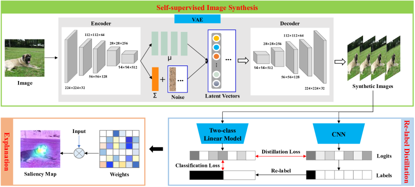
To this end, we propose a re-label distillation approach to interpret the prediction of deep networks. As shown in Fig. 1, we first generate some synthetic images to characterize the feature distribution of the image, and then re-label these synthetic images through a pre-trained DNN to capture the local classification knowledge near the image [9]. In this way, we can transfer the decision boundary knowledge into these re-labeled synthetic images. The interpretation of the prediction can be easily achieved by learning the deconstructed boundary knowledge in an understandable way. Based on this, we train an interpretable model in low-dimensional space with these re-labeled images by distilling the boundary knowledge of DNN [10]. The trained student model learns a direct map from the image to the prediction, which can mark the important features contributed to its prediction. Therefore, the proposed re-label distillation approach can interpret the predictions of deep networks. To validate the effectiveness of our approach, we conduct experiments through qualitative and quantitative evaluations and our re-label distillation approach performs impressively for explanations.
To summarize, the main contributions are as follows: 1) This paper proposes a re-label distillation approach to interpret the predictions of deep networks by distilling into an interpretable model in low-dimensional space; 2) The proposed approach designs an algorithm to train a two-class linear model for explanation. We first generate some synthetic images to represent the classification knowledge of DNN with a VAE. And then we re-label them by identifying whether their predictions shift, which could transfer the boundary knowledge of DNN into them. Finally, we train a two-class linear model through distillation with these re-labeled synthetic images; 3) The experimental results verify the effectiveness of our proposed interpretable approach qualitatively and quantitatively.
2 Approach
The overview of our interpretable approach is illustrated in Fig. 2. In the following subsections, we will analyse the proposed re-label distillation approach in details.
2.1 Problem Formulation
Inspired by transfer learning, we can not only transfer the model structure, but also transfer the interpretability of deep networks. Through some interpretable models, such as linear models or decision trees, deep networks can be reconstructed by distilling their hidden knowledge into these interpretable models. We train an interpretable model to learn the output of the black-box model, so that we can establish an interpretable relationship between the input and output of the black-box model and achieve the interpretability of the predictions.
However, there are two fundamental problems: 1) The nonlinearity of DNN makes it hard to find a perfect interpretable model to capture the entire classification mechanism; 2) Traditional knowledge distillation leads to the loss of a lot of effective information and seriously affects the performance of the student. In order to solve the problems, we generate some synthetic images to represent the classification knowledge of deep networks, and then transfer the local boundary knowledge of the input into an interpretable model. Therefore, we could understand and reason the predictions of DNN.
The foundation of our interpretable approach is mainly to train an interpretable student model to interpret the prediction of a pre-trained DNN with respect to a given image . The student model can learn a direct map from the image to the prediction ,
| (1) |
where can mark the location of the effective features contributed to its prediction. Therefore, we use the parameters of the student as the weight of the features contributed to its prediction, which can be achieved by learning a student to imitate the DNN. In this way, we need some synthetic images to capture the informative classification knowledge towards the DNN. A generator can reconstruct the image to generate some synthetic images for the training of the student.
To formalize the idea of matching the outputs between the student model and the teacher model, we minimize an objective function to match the probability distributions and the outputs of the student with that of the teacher. The loss function for the training of student can be defined as,
| (2) |
where is the cross-entropy classification loss, denotes the student’s prediction distribution with the training parameter , and denotes the teacher’s distribution. Therefore, we can train an interpretable model with some synthetic images to interpret the predictions of deep networks.
2.2 Self-supervised Image Synthesis
In our interpretable framework, the role of the synthetic images is to characterize the classification mechanism of the deep network. The clarity of the synthetic images is not our focus, and we prefer to generate semantically meaningful images of different categories. So we use variational autoencoder (VAE) [11] as this generator. A VAE comprises two sub-networks of an encoder and a decoder . The aim of encoder is to learn a latent representation that describes each latent attribute in probabilistic terms. To generate the synthetic images , we add some random noise to the latent vector,
| (3) |
where and are the mean and standard deviation towards the learned representation of the encoder. The input of our decoder model can be generated by randomly sampling from each latent representation, and the reconstructed output of the decoder is,
| (4) |
where is the training parameter of the decoder .
When training a VAE, we expect the decoder to be able to reconstruct the given input as accurately as possible for any sampling of the latent distributions. Therefore, the values that are close to each other in the latent space should correspond to very similar reconstructions. The training process of a VAE can be formulated as,
| (5) |
where is the parameter of the encoder, measures the similarity between the learned latent distribution and the true prior distribution . The training of VAE is regularised to avoid over-fitting and ensure that the latent space has good properties to enable generative process.
2.3 Re-label Distillation
In order to understand and reason the predictions of deep networks, we use knowledge distillation [19] to train an interpretable model by deconstructing the hidden knowledge inside the teacher, which could achieve an interpretable prediction for a given image. Based on the above analysis, we apply a VAE to generate some synthetic images regarding a specific image and transfer the classification knowledge of deep networks into them. Therefore, we propose the re-label distillation approach to interpret its prediction.
The mathematical description of the re-label distillation will be described below. We feed these re-labeled synthetic images to a pre-trained deep network and re-label them into two class by identifying whether their predictions shift. The predictions of these synthetic images from the teacher are referred as their true labels. In this way, these reconstructed labels include the classification boundary knowledge of the deep network and can be seen as the relation of these predicted labels with respect to the synthetic images. And the synthetic images are re-labeled by
| (6) |
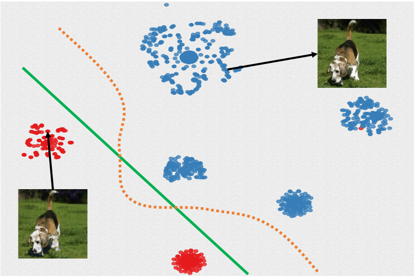
As shown in Fig. 3, these synthetic images can be classified based on the t-SNE [12] plots on ResNet50, which means the classification boundary knowledge of DNN has been transferred to these re-labeled synthetic images. Then, we train a two-class linear model with these re-labeled synthetic images by distilling the soft knowledge of the deep network.
The loss of our proposed re-label distillation to train the student model can be defined as,
| (7) | ||||
where denotes the weights of the linear model, and are the weight coefficients, denotes the prediction of the student model. The trained linear model establishes an interpretable relation between the prediction and the input. The weights could measure the significance of different pixels contributed to its prediction. Therefore, we could obtain an explanation by locating the salient features onto the image.
| Metrics | Methods | Grad-CAM [16] | Sliding Window [18] | LIME [20] | RISE [13] | FGVis [21] | Our method |
|---|---|---|---|---|---|---|---|
| Deletion | ResNet50 | 0.1421 | 0.1232 | 0.1217 | 0.1076 | 0.0644 | 0.0627 |
| VGG16 | 0.1158 | 0.1087 | 0.1014 | 0.0980 | 0.0636 | 0.0513 | |
| Insertion | ResNet50 | 0.6766 | 0.6618 | 0.6940 | 0.7267 | - | 0.7190 |
| VGG16 | 0.6149 | 0.5917 | 0.6167 | 0.6663 | - | 0.7981 |
3 Experiments
To evaluate our re-label distillation approach, we compare with 8 state-of-the-art interpretable approaches in 2 typical deep networks (ResNet50 and VGG16 trained on ImageNet), including RISE [13], Excitation backprop [14], Extremal perturbations [15], Grad-CAM [16], Score-CAM [17], Occlusion sensitivity [18], LIME [20], and FGVis [21].
3.1 Experiment Settings
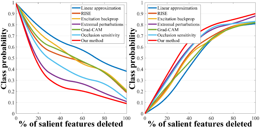
We provide a comprehensive evaluation for our approach qualitatively and quantitatively. The images of ImageNet are preprocessed to 224 224 3 to train our interpretable framework. We use a VAE of 500D latent space to generate 1000 synthetic images for each input by perturbing the latent vector with some random noise. And the coefficients of the re-label distillation loss and are set to 0.7 and 0.3 in Eq.(7). Qualitative evaluation is mainly carried out through the visualization of saliency maps, which present the important features contributed to the predictions. And quantitative evaluation uses the metrics of deletion and insertion [13]. The deletion metric measures the decrease of the prediction probability as more and more salient features are removed from the image, while the insertion measures the increase of the prediction probability as more and more features are inserted.
3.2 Qualitative Results
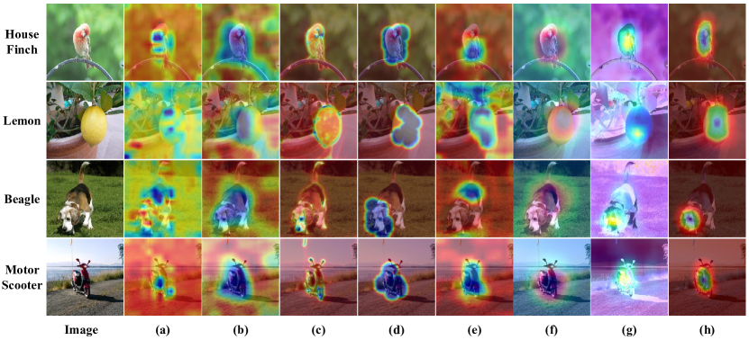
We could explain the decision-making process of deep networks by generating a saliency map, which colors each pixel according to its importance to the prediction. Based on this, we use the weight parameters of the trained linear model to generate the feature-importance maps for qualitative evaluation. As shown in Fig. 4, our re-label distillation approach can mark the significant regions contributed and ignore some irrelevant background information. And compared with other state-of-the-art methods, our saliency map could mark the more accurate target area. Although extremal perturbations [15] could generate an accurate saliency map, our method also shows the importance of these salient features more clearly. By visualizing the saliency map, we can observe the important pixels of the image contributed to its prediction and build an interpretable relationship between them. Therefore, our proposed re-label distillation approach has a better performance in explaining the predictions of deep networks.
3.3 Quantitative Results
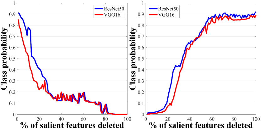
To conduct the quantitative experiments, we use the deletion and insertion metrics to evaluate the saliency maps generated with re-label distillation, and also compare the results with other interpretable approaches. As shown in Fig. 5, the obvious change of the class probability indicates the significance of the salient features towards the predictions of ResNet50 and VGG16. Fig. 6 presents the comparison results with other methods on ResNet50. From the graph above we can see that the class probability is more sensitive to the changes (deletion and insertion) of the salient features under our method. Tab. 1 provides the comparison results of the deletion and insertion metrics averaged on the ImageNet validation dataset. The baseline results are taken from [13]. We use the AUC (area under curve) to measure these two metrics, which means the lower deletion and the higher insertion represent a better explanation. The table above illustrates that our deletion metric is 0.0627 on ResNet50 and 0.0513 on VGG16, and our insertion metric is 0.7190 on ResNet50 and 0.7981 on VGG16. We have achieved significantly better results, and there is only a small gap compared with RISE [13] on the insertion of VGG16. Our saliency map has a greater impact on the prediction probability from deep networks, which confirms that the re-label distillation approach could generate a more accurate explanation than others. Therefore, the re-label distillation generally outperforms these interpretable methods.
4 Conclusion
In this paper, we propose a re-label distillation approach to interpret the predictions of deep networks. We first apply a VAE to generate some synthetic images. Then, we feed these synthetic images into deep networks for the reconstructed labels which are annotated by identifying whether they shift. Finally, we train a two-class linear model on these re-labeled synthetic images by distilling the soft logits and the hard labels. Therefore, the trained linear model learns a direct map to locate the salient features of the input towards its corresponding prediction. The experiments demonstrate that our approach can interpret the predictions of deep networks better. And this work also provides research ideas for the future development of explainable artificial intelligence.
References
- [1] Seyran Khademi, Xiangwei Shi, Tino Mager, Ronald Siebes, Carola Hein, Victor de Boer, and Jan van Gemert, “Sight-seeing in the eyes of deep neural networks,” IEEE International Conference on e-Science, pp. 407–408, 2018.
- [2] A B Arrieta, Natalia Díaz-Rodríguez, Javier Del Ser, A Bennetot, and F Herrera, “Explainable Artificial Intelligence (XAI): Concepts, Taxonomies, Opportunities and Challenges toward Responsible AI,” Information Fusion, vol. 58, pp. 82–115, 2020.
- [3] Christoph Molnar, Giuseppe Casalicchio, and Bernd Bischl, “Interpretable Machine Learning – A Brief History, State-of-the-Art and Challenges,” European Conference on Machine Learning and Principles and Practice of Knowledge Discovery in Databases Workshops, pp. 417–431, 2020.
- [4] Gabriëlle Ras, Marcel van Gerven, and Pim Haselager, “Explanation Methods in Deep Learning: Users, Values, Concerns and Challenges,” Explainable and Interpretable Models in Computer Vision and Machine Learning, pp. 19–36, 2018.
- [5] Quan shi Zhang and Song chun Zhu, “Visual interpretability for deep learning: a survey,” Frontiers of Information Technology and Electronic Engineering, vol. 19, pp. 27–39, 2018.
- [6] Cher B, Mariana da S, Carole H. Sudre, Petru-Daniel T, Stephen M. S, and Emma C. R, “ICAM: Interpretable Classification via Disentangled Representations and Feature Attribution Mapping,” Advances in Neural Information Processing Systems, vol. 33, pp. 7697–7709, 2020.
- [7] Katherine G, Daniel R, and Joshua Z, “Explaining Neural Network Predictions for Functional Data Using Principal Component Analysis and Feature Importance,” arXiv:2010.12063, 2020.
- [8] Yu Zhang, Peter Tiño, Ales Leonardis, and Ke Tang, “A Survey on Neural Network Interpretability,” arXiv: 2012.14261, 2020.
- [9] Junpeng Wang, Liang Gou, Wei Zhang, Hao Yang, and Han Wei Shen, “DeepVID: deep visual interpretation and diagnosis for image classifiers via knowledge distillation,” IEEE Transactions on Visualization and Computer Graphics, vol. 25, pp. 2168–2180, 2019.
- [10] X Liu, Xiaoguang Wang, and S Matwin, “Improving the interpretability of deep neural networks with knowledge distillation,” International Conference on Data Mining Workshops, pp. 905–912, 2019.
- [11] Matt J Kusner, Brooks Paige, and Jose Miguel Hernandezlobato, “Grammar variational autoencoder,” International Conference on Machine Learning, pp. 1945–1954, 2017.
- [12] Laurens van der Maaten and Geoffrey Hinton, “Visualizing data using t-sne,” Journal of Machine Learning Research, vol. 9, pp. 2579–2605, 2008.
- [13] Vitali Petsiuk, Abir Das, and Kate Saenko, “RISE: Randomized Input Sampling for Explanation of Black-box Models,” British Machine Vision Conference, p. 151, 2018.
- [14] Jianming Zhang, Zhe L. Lin, Jonathan Brandt, Xiaohui Shen, and Stan Sclaroff, “Top-Down Neural Attention by Excitation Backprop,” International Journal of Computer Vision, vol. 126, no. 10, pp. 1084–1102, 2018.
- [15] Ruth Fong, Mandela Patrick, and Andrea Vedaldi, “Understanding Deep Networks via Extremal Perturbations and Smooth Masks,” IEEE International Conference on Computer Vision, pp. 2950–2958, 2019.
- [16] Ramprasaath R. Selvaraju, Michael Cogswell, Abhishek Das, Ramakrishna Vedantam, Devi Parikh, and Dhruv Batra, “Grad-CAM: Visual Explanations from Deep Networks via Gradient-Based Localization,” International Journal of Computer Vision, vol. 128, no. 2, pp. 336–359, 2020.
- [17] Haofan Wang, Zifan Wang, Mengnan Du, Fan Yang, and Xia Hu, “Score-CAM: Score-Weighted Visual Explanations for Convolutional Neural Networks,” IEEE Conference on Computer Vision and Pattern Recognition Workshops, pp. 111–119, 2020.
- [18] Matthew D. Zeiler and Rob Fergus, “Visualizing and Understanding Convolutional Networks,” European Conference on Computer Vision, pp. 818–833, 2014.
- [19] G. Hinton, O. Vinyals, and J. Dean, “Distilling the knowledge in a neural network,” Advances in Neural Information Processing Systems Workshop, pp. 1–9, 2014.
- [20] Marco Tulio R, S Singh, and C Guestrin, “’Why Should I Trust You?’: Explaining the Predictions of Any Classifier,” ACM SIGKDD International Conference on Knowledge Discovery and Data Mining, pp. 1135–1144, 2016.
- [21] Jorg Wagner, Jan Mathias Kohler, Tobias Gindele, Leon Hetzel, Jakob Thaddaus Wiedemer, and Sven Behnke, “Interpretable and Fine-Grained Visual Explanations for Convolutional Neural Networks,” IEEE Conference on Computer Vision and Pattern Recognition, pp. 9097–9107, 2019.