The Scuti stars of the Cep–Her Complex. I: Pulsator fraction, rotation, asteroseismic large spacings, and the relation
Abstract
We identify delta Scuti pulsators amongst members of the recently-discovered Cep–Her Complex using light curves from the Transiting Exoplanet Survey Satellite (TESS). We use Gaia colours and magnitudes to isolate a subsample of provisional Cep–Her members that are located in a narrow band on the colour–magnitude diagram compatible with the zero-age main sequence. The Sct pulsator fraction amongst these stars peaks at 100% and we describe a trend of higher pulsator fractions for younger stellar associations. We use four methods to measure the frequency of maximum amplitude or power, , to minimise methodological bias and we demonstrate their sound performance. The measurements display a correlation with effective temperature, but with scatter that is too large for the relation to be useful. We find two ridges in the – diagram, one of which appears to be the result of rapid rotation causing stars to pulsate in low-order modes. We measure the values of Sct stars in four other clusters or associations of similar age (Trumpler 10, the Pleiades, NGC 2516, and Praesepe) and find similar behaviour with . Using échelle diagrams we measure the asteroseismic large spacing, , for 70 stars, and find a correlation between , rotation, and luminosity that allows rapid rotators seen at low inclinations to be distinguished from slow rotators. We find that rapid rotators are more likely than slow rotators to pulsate, but they do so with less regular pulsation patterns. We also investigate the reliability of Gaia’s vbroad measurement for A-type stars, finding that it is mostly accurate but underestimates for slow rotators ( km s-1) by 10–15%.
keywords:
asteroseismology – stars: evolution – stars: fundamental parameters – open clusters and associations: individual: Cep–Her – stars: variables: Scuti1 Introduction
Asteroseismology of star clusters has long held great promise. The idea is simple: with ensemble asteroseismology, one aims to use multiple stars to achieve the same modelling goal, most commonly a cluster age measurement (Basu et al., 2011). Historically, the motivation arose from it being much easier to measure distances to clusters than to lone stars (Breger, 2000). Now, with Gaia (Gaia Collaboration et al., 2023), we can measure distances to individual stars accurately (Bailer-Jones et al., 2021),111Incidentally, those distances can be verified asteroseismically for red giants, e.g. Zinn et al. (2018); Khan et al. (2023). and also use those distances and kinematics to establish cluster membership (Pang et al., 2022; Hunt & Reffert, 2023; Kerr et al., 2023). In addition, clusters can now be treated with hierarchical Bayesian modelling, where not only are the stars assumed to have the same target distribution in age and metallicity, but each individual star also contributes to the overall prior (Olivares et al., 2018; Lyttle et al., 2021).
Cluster asteroseismology has delivered several significant results in recent years, especially from the study of red giants (RGs). Brogaard et al. (2023) found empirical evidence for the long-standing expectation that rotational mixing and core overshooting affect main-sequence lifetimes, and hence cluster age measurements, via the study of RGs in NGC 6866 (see also Hidalgo et al. 2018). It is widely known that ancient globular clusters have subpopulations or have had multiple generations of star formation (see the review by Bastian & Lardo 2018), and asteroseismic evidence of this has been found in the globular clusters M4 (Tailo et al., 2022) and M80 (Howell et al., 2024), as well as in some massive open clusters (Sandquist et al., 2020). Clusters have also been used to verify the asteroseismic scaling relations for RGs (e.g. Brogaard et al., 2016), while asteroseismology has been able to identify former (escaped) members of open clusters (Brogaard et al. 2021; see also Heyl et al. 2022; Bedding et al. 2023).
The pulsations of intermediate-mass main-sequence members of star clusters have been somewhat less studied, except perhaps for the broad attention historically given to blue stragglers (Bailyn, 1995; Pych et al., 2001; Templeton et al., 2002; Jeon et al., 2004; Poretti et al., 2008; McNamara, 2011; Stȩpień et al., 2017). With the Transiting Exoplanet Survey Satellite (TESS) collecting photometry of most of the sky, asteroseismology of A stars on or near the main-sequence ( Sct stars) in clusters has undergone a renaissance, most notably for the Pleiades, but also for Praesepe, Per, and others (Kerr et al., 2022a, b; Murphy et al., 2022; Bedding et al., 2023; Pamos Ortega et al., 2022; Pamos Ortega et al., 2023). This is no surprise, given that clusters might hold the answers to important questions that are especially pertinent to A-type stars, such as the origin and efficiency of angular momentum transport in stars (Aerts et al., 2019; den Hartogh et al., 2020), the origin and prevalence of chemical peculiarities with age (Palla & Stahler, 2000; Stȩpień, 2000; Gray & Corbally, 2002; Fossati et al., 2007; Smalley et al., 2017), and how the Sct pulsator fraction changes with age (Murphy et al., 2019; Bedding et al., 2023). The latter is a topic we address in this work.
In this work we also study the – relation for Sct stars. It has long been known that hotter Sct stars tend to pulsate in higher radial overtones (Breger & Bregman, 1975). While a relation is well-tested and widely exploited in solar-like oscillators (e.g. Stello et al., 2009; Coelho et al., 2015; Yu et al., 2018), such a relation for Sct stars has so far produced correlations with large scatter (Bowman & Kurtz, 2018; Barceló Forteza et al., 2018, 2020; Hasanzadeh et al., 2021). Those studies focussed on analysing large datasets of Kepler and TESS photometry for heterogeneous samples of stars, so it remains unclear whether the scatter is a consequence of the broad range of encompassed physical parameters (most notably metallicity and age), or from idiosyncrasies of the driving and damping of pulsations in Sct stars, which might pose a fundamental limit on the available precision of the relation. A recent change in direction has been to study a homogeneous sample, such as that offered by 36 Sct stars in the Pleiades star cluster (Bedding et al., 2023), for which a scaling relation seems doubtful, and 35 Sct stars in NGC 2516 (Li et al., 2023), wherein a relation appears for about a dozen stars within a narrow colour range. In this work, we use 195 Sct stars in the Cep–Her association to isolate a homogeneous sample in metallicity and age with which to revisit the question of whether a – relation exists for Sct stars.
Cep–Her contains at least four kinematically distinct associations or subgroups (Kerr et al., submitted), and is sometimes referred to as the Cep–Her Complex. We use the latter term only when the scope of different subgroups is relevant. All subgroups within the Complex are younger than 100 Myr (Kerr et al.; and Sec. 2.1 below). There are no red giants or other viable solar-like oscillators with which to determine asteroseismic ages. The stars are also younger than the empirical limit of gyrochronology (Bouma et al., 2023; Lu et al., 2023). Existing age solutions in Cep-Her are computed almost entirely using isochronal ages, which can vary by more than a factor of two depending on the choice of model (Herczeg & Hillenbrand 2015; Kerr et al., submitted). As such, new methods with more reliable absolute scaling are necessary to better constrain the ages of the many substructures in Cep-Her. Independent asteroseismic ages for these subgroups would be valuable, and will be the topic of Paper II. In this work, we identify the Cep–Her members that pulsate as Sct stars, collate their physical parameters, and measure their asteroseismic large spacing where possible.
2 Methodology
2.1 Stellar parameters and association membership
Our stellar sample is based on the Kerr et al. (2023) Cep–Her membership list. This catalogue includes basic stellar properties for all candidate members including Gaia photometry, distances from Bailer-Jones et al. (2021), reddening estimates derived from the Lallement et al. (2019) reddening maps, and membership probability estimates based on the relative populations of nearby photometrically young and old stars. We required , removing probable non-members from the sample. The photometry, distances, and reddening can be combined to produce absolute values of Gaia colour and absolute magnitude. We required de-reddened Gaia colour , as well as Gaia absolute magnitude , limiting the population to the range of temperatures where pulsators are typically found, while using the cut on to remove dim stars with poor photometry, as well as any white dwarfs. From a list of 986 Gaia targets after these cuts, we successfully cross-matched TIC numbers for 958 stars, constituting our final sample. The other 28 stars had been resolved into duplicated TIC numbers.
The Cep–Her Complex has recently been found to contain four sub-components with distinct dynamics and ages: Cinyras, Orpheus, Cupavo, and Roslund 6 (Kerr et al., submitted). The Cinyras and Orpheus Associations have PARSEC isochronal ages that span 28-43 Myr and 25-40 Myr, respectively, while while Cupavo has ages between 54 and 80 Myr and Roslund 6 may be older than 100 Myr. Of the stars in this sample, 205 lie in Cinyras, 478 are in Orpheus, 249 are in Cupavo, and 54 are in Roslund 6. The sample therefore spans only a small range of ages corresponding to 5% of the main-sequence lifetime.
We used the Gaia DR3 IDs to extract the Renormalised Unit Weight Error (ruwe) from the Gaia DR3 catalogue (Gaia Collaboration et al., 2023). High ruwe values are indicative of unresolved binaries (Evans, 2018; Rizzuto et al., 2018; Belokurov et al., 2020; Stassun & Torres, 2021; Penoyre et al., 2022), but not with 100% reliability (Gallenne et al. 2023; Dholakia et al. in prep.). We also note that circumstellar disk material can inflate ruwe values for single stars (Fitton et al., 2022), so ruwe values for stars in young associations might be inflated on average when compared to older populations, even after accounting for the dynamical evaporation of binary systems on timescales of hundreds of Myr (Fujii et al., 2012). We therefore stopped short of assigning a binarity flag based on ruwe values, but we did consider ruwe values as approximate indicators of binarity in conjunction with other observations where appropriate.
Also from Gaia DR3, we extracted the vbroad and vbroad_error values where available. Since A stars often rotate rapidly, with a mean in excess of 100 km s-1 (Royer et al., 2007), the total line broadening is dominated by rotation. Hence, rapid rotators in our sample will have large values of vbroad (unless seen from low inclinations) and slow rotators will not (see also Gootkin et al. 2024). Rotation causes a deformation that scales as the square of the angular rotation frequency, (). The resulting decrease in stellar density has two consequences important to this work: firstly, it means that rotating models are required to model these Sct stars (see discussion in Murphy et al. 2022); and secondly, the corresponding decrease in effective temperature pushes rapid rotators to the right (and sometimes up, depending on inclination) on the colour-magnitude diagram (Pérez Hernández et al., 1999; Bedding et al., 2023). We evaluate the reliability of vbroad for Sct stars in Sec. 5.2.
Stellar effective temperatures () and their uncertainties were taken from the TESS Input Catalogue (TIC; Stassun et al. 2019). The TIC temperatures were calculated from spectroscopy originating from nine catalogues covering over 3 million sources, and were supplemented with photometry where required (see Stassun et al. 2019 for details). For our targets, the median uncertainty is 156 K, which is rather low compared to the calibration of the scale with interferometry (Casagrande et al., 2014; White et al., 2018). However, these uncertainties are merely indicative and do not underpin our analysis. Note that we did not use Gaia DR3 gspphot temperatures because 19 per cent of our sample had no available values in this catalogue. The situation was worse for gspspec temperatures (90 per cent missing). Instead, we used both TIC and de-reddened Gaia colour, and we provide them with other stellar parameters online and in the Appendix (Table A) for the subset of stars analysed in detail in this work (sample selection is described in Sec. 2.3 and Sec. 2.6). The Gaia colour is a reliable and widely-available temperature proxy.
2.2 Downloading TESS lightcurves
We used light curves from the Transiting Exoplanet Survey Satellite (TESS; Ricker et al. 2015). These lightcurves are now available in a variety of cadences. During the first two years of the TESS mission, stars were observed either in 2-min cadence, or were available through custom lightcurves created from Full Frame Images (FFIs) taken at 30-min cadence. In the first extended mission, the FFI cadence reduced to 10-min (Bell, 2020), and these light curves are now available for many stars as official data products made by the Science Processing Operations Centre (SPOC; Jenkins et al. 2016). The FFI cadence was reduced again to 200 s in the second extended mission. A 20-s cadence is also available for a smaller number of stars.
In this work, we used 2-min cadence light curves when available, and the 10-min FFI light curves otherwise, using the SPOC light curves in both cases. We did not mix cadences for any individual target, did not create any custom lightcuves, and used neither the 20-s nor the 200-s cadences as there were comparatively few Cep–Her targets available in these cadences. Where multiple sectors were available for a given star at the same cadence, we combined those sectors without any adjustment of the times (Bedding & Kjeldsen, 2022). Most of the light curves we collated have data from one sector (24%) or two sectors (69%), with a minority having three (1%) or four (5%) sectors. All lightcurves were retrieved with the lightkurve package (Lightkurve Collaboration et al., 2018).
2.3 Identifying variable stars
To identify Sct variables in the association, we calculated the amplitude spectrum for each light curve with the Lomb–Scargle periodogram (Lomb, 1976; Scargle, 1982) implemented in astropy (Astropy Collaboration et al., 2022). For stars with only 10-min FFIs we used the Nyquist frequency (72 d-1) as the upper frequency limit of the calculation, whereas for the 2-min lightcurves we used 90 d-1. In both cases the lower limit was 10 d-1 and the frequency resolution was set as , where is the timespan of the data. The lower limit was justified via both the Period–Luminosity relation and stellar models, which indicate the fundamental radial mode should lie above about 15 d-1 (Ziaali et al., 2019; Barac et al., 2022; Murphy et al., 2023).
Stars whose amplitude spectra have high skewness are most likely pulsators (Murphy et al., 2019; Barbara et al., 2022; Read et al., 2024), whereas low skewness is suggestive of white noise. We measured the skewness of the amplitude array at frequencies above 15 d-1. Given the potential for spectral leakage or harmonics, this lower limit in frequency was necessary to distinguish Sct stars from other classes whose variability is found at lower frequencies, such as SPB stars, Dor stars, and eclipsing binaries. We found the distribution of the resulting skewness values was bimodal, comprising non-variables with , and Sct stars with (Fig. 1). We automatically assigned a ‘dSct’ flag to all 188 stars with , but visually checked the 88 stars with and reassigned any misclassifications (16 additional stars given ‘dSct’ flag, 9 stars had their flag removed). Ambiguous cases were left with their original (automated) assignations. The result was 195 stars labelled as ‘dSct’.
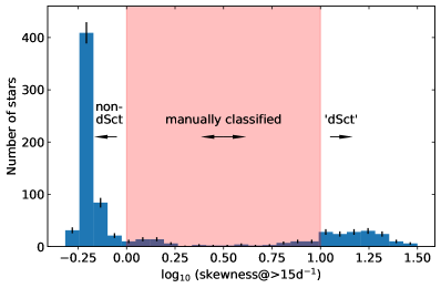
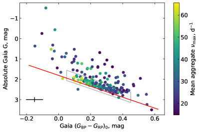
Fig. 2 shows the colour–magnitude diagram of Cep–Her with the Sct stars identified. The bottom panel reveals that most of the Sct stars form a tight group, which could be interpreted as young stars immediately after the ZAMS that have just started fusing hydrogen. This ZAMS group, as we shall refer to it, is tighter in de-reddened colour than in TIC , hence we continue to use colour in our analysis. We define the ZAMS group explicitly in Sec. 2.6.
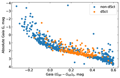
Within the ZAMS group, the small spread in brightness for a given colour is attributable to small age differences, or differences in rotation rate and the corresponding oblateness thus imposed. There is also a contribution from observational uncertainty: the pulsators have median uncertainties on and of 0.051 mag and 0.098 mag, respectively, mostly originating from unknown extinction and associated reddening, although the uncertainties are dominated by systematic rather than random effects. The fact that the formal uncertainties in Fig. 4 are larger than the apparent scatter perhaps indicates that the extinction map uncertainties are overestimated.
Beyond the bright (upper) end of the ZAMS group lie many stars with high ruwe, which are easily explained as binaries. There are many other stars that are around 1 mag brighter than the ZAMS group, which do not have high ruwe values. If their parallaxes are correct, these are probably not binaries, but Gaia is known to underestimate parallaxes (overestimate distances) to unresolved binaries in some cases (e.g. Lee, 2021), giving the impression they are much brighter than they are. It probable that many of these stars do not belong to Cep–Her. To avoid them affecting our statistics, we focus our analyses on the ZAMS group.
2.4 Extracting mode frequencies
For the Sct stars, we determined mode frequencies via iterative prewhitening in a custom-written script,222https://github.com/gautam-404/pre-whiten which iteratively fits sinusoids corresponding to peaks in the amplitude spectrum. Starting with the highest peak, the function fits for its frequency, amplitude, and phase, then subtracts it from the light curve. Iterations continue until a specified Signal-to-Noise Ratio (SNR) threshold is reached. The SNR is the ratio of the maximum amplitude in a given iteration to the median Fourier amplitude at that iteration.
Key thresholds and parameters incorporated within this module include:
-
•
snr_threshold: Dictates the SNR threshold for terminating iterations: if the -th peak has a SNR below this threshold, iterations cease and the -th peak is discarded. We used the default value of 5.
-
•
nearby_tolerance: Specifies the permissible proximity between two frequencies before they are deemed overlapping. Ideally, i.e. in the case of a finite uninterrupted time-series of high signal-to-noise, this tolerance should be approximately the Rayleigh resolution (), where is the observational time span. Our TESS light curves have T ranging from 27 d to over 1000 d, but for consistency we adopted a criterion of 0.01 d-1 as our nearby_tolerance. No peaks were sought at a frequency separation less than this from an existing peak.
-
•
harmonic_tolerance: Determines the proximity between the frequency of a trial peak and an integer multiple of a different frequency, below which the trial peak would be deemed a harmonic. This tolerance is often set to a small frequency difference (typically smaller than , e.g. Uzundag et al. 2023), or a small fraction (say 1%) of combination peak’s frequency. This ensures that if, for example, one frequency is approximately twice (within 1% deviation) another frequency, it is considered its harmonic and flagged as such. Since we were primarily interested in variability and not the relationship between peaks, we did not use this option.
-
•
max_iterations: The maximum number of allowed iterations. We used the default value of 100.
The full documentation can be found in the readme.
2.5 Measuring
By analogy with solar-like oscillations (Kjeldsen & Bedding, 1995), we use to characterize the central frequency of the oscillations. It is important to keep in mind that there is no single definition of , even for solar-like oscillations (Hekker, 2020; Sreenivas et al., 2024), and the situation is even more ambiguous for Sct stars because of their uneven distribution of peak heights. We measured in a variety of ways to compare approaches and to ascertain a methodological uncertainty. The random uncertainty on each method is very small, because the modes of Sct stars are mostly coherent and of fairly constant amplitude (Murphy et al., 2014; Bowman et al., 2016). However, the way in which is determined can lead to differences of 10 per cent. The simplest definition is to use the strongest peak, but Sct stars can have modes excited at several radial orders (Antoci et al., 2011; Murphy et al., 2023), and the strongest peak seldom lies at the centre of the envelope of excited peaks (e.g. Bedding et al., 2023). One can use a number of peaks to calculate an average, either in power or amplitude.
We have measured in five different ways. The first, which we refer to as , is simply the frequency of the strongest peak. Note that is the same in amplitude and in power. We refer to the other four methods as ‘aggregate’ methods because they use all significant peaks. These aggregate methods all used 10 d-1 as the lower frequency limit.
The second method calculates the moment of the extracted mode frequencies, , weighted by their amplitudes, (measured in Sec. 2.4):
| (1) |
This is the method used by Barceló Forteza et al. (2018). The third method is identical to the second, except that it is calculated using power () instead of amplitude. The use of power is physically motivated, because the energy contained within a given mode is proportional to the power, rather than the amplitude.
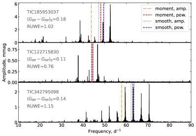
The fourth and fifth approaches were to heavily smooth the amplitude and power spectra by convolving with a broad Gaussian and measuring the peak of the resulting envelope. In studies of solar-like oscillations in main-sequence stars, a Gaussian of width is typically used (Kjeldsen et al., 2005, 2008). Here, we used a width of 30 d-1, being about four times the of the high-frequency Sct stars in the association.333Convolution can be done with astropy.convolve_fft on a Gaussian1DKernel. The fft algorithm is much faster than convolve for larger smoothing windows. This approach requires the white noise to be subtracted first, lest the result be dominated by a spectrum of mostly noise in low-amplitude pulsators. For this, we measured the mean amplitude at each end of the Fourier data, and d-1, and took the lesser of these two values as the mean noise for each star separately. We subtracted this from each element of the amplitude array, allowing negative amplitudes. Naturally, in both the moment and the smoothing method, the use of power will tend to bias the result towards the strongest peaks rather than a plethora of small ones. An example is provided in Fig. 3.
Values of resulting from all five methods are given in Table A. For some stars, all four aggregate methods agree well (as tightly as 0.06 d-1), whereas for others there is substantial spread (up to 13.76 d-1). The standard deviations of the aggregate methods around their collective mean are 1.90 (moment method in amplitude), 1.21 (moment method in power), 2.48 (smoothing method in amplitude), and 1.95 d-1 (smoothing method in power). (For the frequency of maximum amplitude, the standard deviation is 4.49 d-1.) We adopted the mean of the four aggregate methods hereafter.
2.6 Defining the ZAMS group
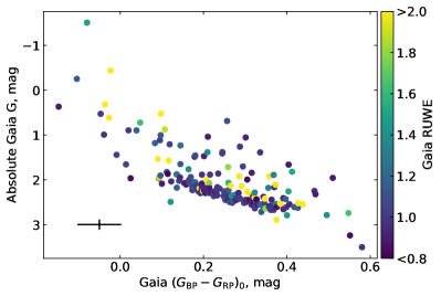
In Fig. 4 we show as measured by the moment (amplitude) method across the colour–magnitude diagram. Amongst the ZAMS group, but not outside it, there is an apparent trend of higher at bluer temperatures, that is, an apparent – relation. We defined the ZAMS group numerically for further analysis, based on their height above the ZAMS, as follows. We first defined a line that roughly locates the ZAMS, by tracing the minimum luminosity of the ZAMS group (red line in Fig. 4), which has the equation
| (2) |
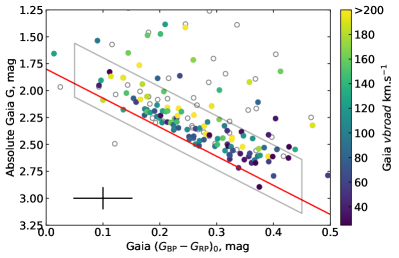
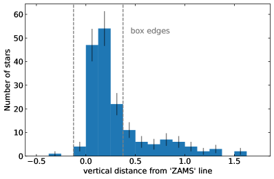
The grey box surrounding it constrains the sample to colours of , which emerged as the natural edge of the population. The vertical height of the box is 0.5 mag, and extends 0.125 mag below the ZAMS to capture slightly fainter stars, such as those that might be partially obscured by circumstellar disks or might have been shifted down by larger-than-average parallax uncertainties. The choice of box height excluded several binaries identified by their ruwe values in Sec. 2.3. The histogram in Fig. 5 shows the vertical distance of stars from the ZAMS line and justifies the edge of the ZAMS group drawn in this manner: above the drawn box, the number of stars per bin falls to a background level, within the uncertainties. We also note the clear tendency of rapid rotators in Fig. 4 to lie farther above the ZAMS line than the slow rotators, as expected. The parameters of the 126 ZAMS-group Sct stars are given in Table A. We investigate their – relation in the next section.
3 The – scaling relation
Solar-like oscillators exhibit a power excess in a roughly Gaussian envelope, inside which all eigenmodes are excited. The observational challenge is to obtain a time-series of sufficient precision, duration and cadence to see them. The centre of this envelope is called and follows one of the asteroseismic scaling relations (Brown et al., 1991; Kjeldsen & Bedding, 1995),
| (3) |
where is the surface gravity (typically measured in solar units). Main-sequence stars, subgiants, and red giants follow this relation quite closely (e.g. Chaplin & Miglio, 2013; Hekker, 2020; Li et al., 2021).
The Sct stars, on the other hand, typically have complex and seemingly disordered amplitude spectra that are not usually contained within a roughly Gaussian envelope (e.g. Guzik, 2021; Ramón-Ballesta et al., 2021). In fact, it only appears to be young Sct stars that provide an exception to this, where comb-like patterns of pulsation modes are sometimes seen (Suárez et al., 2014; Paparó et al., 2016; Michel et al., 2017; Bedding et al., 2020; Murphy et al., 2021, 2022; Steindl et al., 2022; Bedding et al., 2023; Scutt et al., 2023; Murphy et al., 2023). As detailed by Murphy et al. (2023), the reasons for this are becoming understood, which are principally that older stars feature greater interaction between the p and g modes (Christensen-Dalsgaard, 2000; Lignières & Georgeot, 2009; Aerts et al., 2010) and older stars have sharp molecular weight gradients at the edge of the convective core (Reese et al., 2017; Dornan & Lovekin, 2022), both of which spoil regular patterns. But even in these young Sct stars, a true envelope is seldom apparent: Bedding et al. (2023) showed that the distribution of peaks in the amplitude spectra of Sct stars in the Pleiades cluster is not very ordered, even though a correlation is expected between photometric colour (or ) and the excitation of pulsation modes of higher radial orders (Dziembowski, 1997; Pamyatnykh, 2000).
Conversely, studies of large numbers of Sct stars do find the expected correlation between and (Bowman & Kurtz, 2018; Barceló Forteza et al., 2018, 2020; Hasanzadeh et al., 2021). In the open cluster NGC 2516, which has an age of about 100 Myr, Li et al. (2023) found a clear relation between pulsation frequency and colour for a subset of stars in a narrow colour range. We have already shown that there is a correlation in the Cep–Her sample in Sec. 2.6. In this section, we investigate whether differences in method (i.e. systematic uncertainties) might play a role in hiding the correlation, and whether the correlation is useful for estimating stellar properties.
3.1 Systematic uncertainties in measuring
By analysing only stars in the ZAMS group (Sec. 2.3 and 2.6), we have a homogeneous sample in terms of metallicity, surface gravity, and age (within a few tens of Myr). Our sample selection will have preferentially excluded binaries, especially those in which the Sct star is the secondary. Hence, any binaries that remain in the sample should have similar colours to the Sct component they contain, and should not strongly affect any – relation.
In Fig. 6 we show our four aggregate methods (Sec. 2.5) for measuring (omitting the measurement that uses only a single peak) as a function of colour. The figure shows an upper envelope: high values are not found for redder stars, though some blue stars do have low . The linear least-squares fit in the top panel of Fig. 6 is clearly a poor fit to the data. This cannot be explained by sample inhomogeneity, or by measurement uncertainty, because we have been generous in applying different methodologies for measuring and none of these methods has large random uncertainties. At face value, it seems the relation is weak.
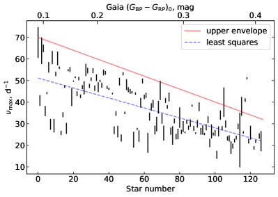
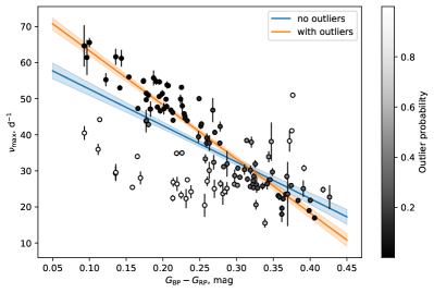
In the middle panel of Fig. 6 we take a more statistical approach. We assume that there is a – relation that is obscured by ‘outlier’ stars that for some unknown reason do not fit the relation. Thus, we generated a mixture model of two populations: those that fit the relation, and those that do not. We used colour as the independent variable, and we used the mean and standard deviation of the four aggregate methods for the data and their uncertainties, respectively.444For the purpose of minimising uncertainty in the modelling process, the data were reparametrized to have a mean of zero in both and , and were transformed back afterwards. The mixture model presumed some stars to follow a – relation modelled with a linear fit whose slope and intercept were free parameters. The background population was modelled as a colour-independent Gaussian in whose mean and standard deviation were free parameters. We also added a jitter term to account for the scatter of points around the relation, which is much larger than the error bars on the data. This was preferred over rescaling the error bars because visual inspection showed that the values and their uncertainties were well determined (see Fig. 3). Finally, we added one additional variable which was the probability of each point being an outlier. We ran this mixture model using a No U-Turns Sampler (NUTS) in numpyro with jax. The sampler used two chains, had 3500 effective samples, and we checked for convergence with the Gelman–Rubin (r̂) statistic using the arviz package. The resulting -colour relation is
| (4) |
which is shown as the orange line in the middle panel of Fig. 6.
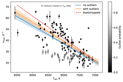
We note that the same model cannot be applied when the independent variable is instead of colour (Fig. 6, bottom) because the distribution of ‘outlier’ stars maps across differently. Specifically, we found that in -space a Gaussian was not a good representation of a background population – it becomes too heavily skewed towards the group of stars with near 25 d-1. Since there is no physically-motivated reason to prefer some other functional form for ‘outliers’, we used the middle panel of Fig. 6 to identify stars with 85% probability of lying on the relation, and used their TIC values to calculate a – relation. From this we found
| (5) |
which is shown as the ‘bootstrapped’ line in the bottom panel of Fig. 6. Note that we did not include a surface gravity term for two reasons. First, unlike solar-like oscillators, Sct stars do not pulsate at frequencies near the acoustic cut-off frequency, and the reason for their pulsation frequencies to depend on is entirely different from solar-like oscillators. Second, our sample is so tightly confined in the colour–magnitude diagram already that no data would be attainable with sufficient accuracy and precision to tighten this relation further.
The origin of the temperature-independent ‘outliers’ remains unclear. We inspected their amplitude spectra to determine whether they were unusual, and to reaffirm that the automated methods to determine had worked correctly. Specifically, we considered the stars with that have a mean d-1. The outliers were unremarkable, and the methods had worked as intended. The examples we showed in Fig. 3 illustrate this well. The top and middle panels show stars that might be considered outliers: they have and d-1, but look like ordinary Sct stars. One of these (middle panel) has all four methods agreeing on the value, whereas the other (top panel) has a wider range of values, but all are reasonable approximations to the centre of the variability. Contrasting the star in the bottom panel of Fig. 3 with the one in the middle panel, we see two stars with low ruwe (presumably single stars) with similar colours (0.14 vs 0.11 mag) but vastly different amplitude spectra.
3.2 Is the – relation useful?
In the TESS era where most Sct stars have light curves available, either from FFIs or otherwise, it would be convenient to be able to use the amplitude spectrum to estimate . This would obviate some of the issues with using colour as a proxy, such as unknown reddening, and might provide tighter and/or more accurate constraints on asteroseismic modelling. This approach has been used to model Sct stars in the open clusters Per (Pamos Ortega et al., 2022), Trumpler 10 and Praesepe (Pamos Ortega et al., 2023). However, we can see that even for stars in the Cep–Her ZAMS group, which represent a homogeneous sample, there can be large outliers in , and stars lying just outside the ZAMS group present an even bigger problem (contrast the of stars inside with those just above the box in Fig. 4).
The standard deviation of points around the – relation of eq. 5 when outliers are excluded is 372 K. (Equivalently, in it is 7.4 d-1.) At 8000 K, which is the median of the sample, this is a 4.7% uncertainty. By comparison, the scale is calibrated by interferometry at the 2% level (Casagrande et al. 2014; White et al. 2018; cf. Miller et al. 2020; Miller et al. 2022), and spectroscopic uncertainties for A stars are typically around 250 K, i.e. 3 per cent, or smaller (e.g. Niemczura et al., 2017; Kahraman Aliçavuş et al., 2020). In this sense, the relation in eq. 5 might offer a useful approximation when no better alternative exists. However, the much larger concern is the presence of the temperature-independent ‘outlier’ population. It is not possible to know to which population a random field star belongs.
Moreover, the 372-K uncertainty corresponded to our careful analysis with robust ‘outlier’ treatment. Suppose that one were to treat the ZAMS group stars as a single population instead, fitting a single linear relation like the dashed-blue line in the top panel of Fig. 6. The scatter (1 standard deviation) would then be 705 K. And if all stars in our initial Cep–Her membership list with and with between 000 K are fitted instead (i.e. temporarily disbanding the ZAMS group), the scatter would equal 1065 K. The instability strip itself is only 2000 K wide (Dupret et al., 2005; Murphy et al., 2019). Hence, we are forced to conclude that although the and of some Sct stars in Cep–Her are correlated, there is no useful relation between them.
3.3 The – relation in other clusters
A handful of clusters have now been studied for evidence of a – relation. Most of these are the same age: Cep–Her spans ages 25–80 Myr, Trumpler-10 has an age of 50 Myr (Kerr et al., 2023), NGC 2516 is around 100-Myr old (Li et al., 2023), and the Pleiades cluster has an age of roughly 125 Myr. Praesepe has also attracted attention, but is substantially older at several hundred Myr. We compare their members’ and values here.
Data were obtained and analysed as uniformly as possible, in the same manner as for Cep–Her. Specifically, we gathered TIC numbers of Sct members and corresponding TIC temperatures from the relevant studies, namely, for 36 stars in the Pleiades from Bedding et al. (2023), for 33 stars in NGC 2516 from Li et al. (2023), and for both 6 stars in Praesepe and 5 stars in Trumpler 10 from Pamos Ortega et al. (2023). With the exception of NGC 2516, for which we requested the custom FFI light curves from the authors, we downloaded 2-min and 10-min TESS light curves in that order of preference as we did for Cep–Her. The four aggregate methods for measuring were applied identically across all clusters. We show the distributions of and TIC in Fig. 7.
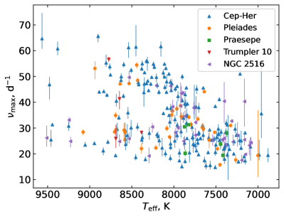
Unlike in Fig. 6, where we focussed on only those stars in the ZAMS group, here all Cep–Her stars in the shown range are plotted, since the membership lists of other clusters were not curated in the same way as the ZAMS group. The – relation is shown in Fig. 7 and some interesting structure is evident. Specifically, very few stars lie in the upper-right portion of the diagram, and stars hotter than K appear to fall on either one of a pair of (non-parallel) ridges.
Briefly, we might explain this as follows: for young clusters like those in Fig. 7, the typical is around 7 d-1 (we show this in Sec. 5.4 for Cep–Her stars), and the fundamental radial mode frequency lies at roughly 3 (Murphy et al., 2023), hence the horizontal (temperature-independent) band of points comprises stars dominated by the fundamental mode. Although the figure covers stars of a wide range of masses, it appears that ZAMS densities of Sct stars are mass-independent (Murphy et al., 2023), unless modified by rotation, hence their values and fundamental mode frequencies are similar across a range of temperatures (masses). Since the fundamental radial mode is the p mode of lowest frequency, modes of the same radial order but different degree as well as modes at the next radial order () will have slightly higher frequencies, which explains why this ridge in the figure constitutes a broadened band between 20 and 30 d-1. The stars that lie on the diagonal band in Fig. 7, whose exhibits temperature dependence, would necessarily oscillate in modes of higher radial order.
The question is then why do some hot Sct stars pulsate predominantly in low radial orders (around the fundamental radial mode) while others pulsate at higher orders? The same question, incidentally, might be applied to the so-called second ridge in the Period–Luminosity relation (Ziaali et al., 2019; Barac et al., 2022). One can speculate that the answer is connected to the different driving mechanisms behind Sct pulsations (Houdek 2000; Antoci et al. 2014; Murphy et al. 2020b), but that only shifts the question to why the same available mechanisms drive oscillations of higher radial orders in some stars of the same temperature than in others.
An answer might be found in studies of roAp stars, for which models whose surface layers are depleted in helium have unstable p modes at higher frequencies than those without helium depletion (Cunha et al., 2013). In other words, the level of helium depletion affects . Suppose this also applies to Sct stars without the (typically strong) magnetic fields seen in roAp stars, which appears to be the case (M. Cunha, private communication). In that case, two predictions follow: (i) unless a substantial amount of helium settling can occur soon after the fully-convective pre-MS phase is over, then older stars (i.e. older clusters) should behave differently from younger ones; and (ii) rapid rotators should behave differently from slow rotators, since helium settling is ineffective in the former due to large scale interior flows (meridional circulation).
The first prediction is unfortunately not addressed by the Praesepe members in Fig. 7. Praesepe is much older than the other clusters but its Sct members are all cooler than 8000 K, hence they do not lie in the part of the diagram where we see two ridges. Another intermediate-age cluster (0.2–0.5 Gyr) is required to evaluate this hypothesis, noting that older clusters will have fewer hot Sct stars (they evolve to cooler ). We could find none with readily available data, and a full analysis of another cluster is beyond the current scope.
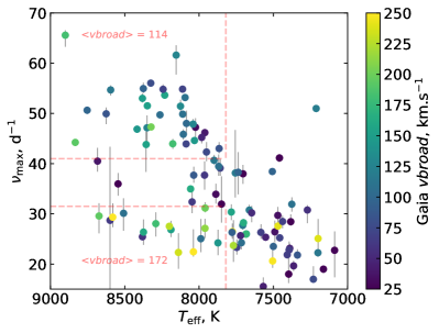
The second prediction can be evaluated with our current data. Using the Cep–Her stars in the ZAMS group that have Gaia vbroad measurements, we observe some dependence on vbroad (Fig. 8). Specifically, the most rapid rotators appear to lie on the bottom ridge. By dividing the plot into areas containing stars that are unambiguously bottom-ridge or top-ridge stars, we see substantial differences in their mean vbroad values, at 172 and 114 km s-1, respectively. The standard deviation around the former mean is 65 km s-1, hence this is only a 1 result. We can say only that there is weak evidence that rapid rotation causes Sct stars to pulsate in low- modes.
4 The Sct pulsator fraction in Cep–Her
Using the ‘dSct’ flag assigned in Sec. 2.3, and evaluating stars within the box containing the ZAMS group on the HRD (Sec. 2.6), we calculated a histogram of the number of pulsators and of the total number of stars () as a function of dereddened colour (Fig. 9). We also show the pulsator fraction, , as the quotient of those quantities. The uncertainty on that quotient is calculated for the -th bin by assuming the measurements comprise a set of binomial trials (also called Bernoulli trials), in which the star is either pulsating or it is not (e.g. Taylor 2022):
| (6) |
We found that the pulsator fraction rises monotonically to its peak in the bin , where it reaches 100%. In , this bin corresponds to K.
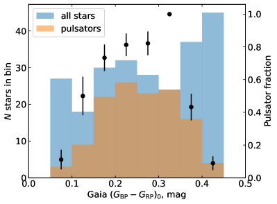
The emerging trend is that younger populations have a higher fraction of Sct stars. The Kepler Sct population from Murphy et al. (2019) comprised over 2000 stars that were slightly out of the Galactic plane, and the distance from the Galactic plane was generally larger for the more distant stars. Their average age is presumably several hundred Myr. Murphy et al. (2019) measured their pulsator fraction as 50–60 per cent in the middle of the instability strip. The 120-Myr Pleiades sample from Bedding et al. (2023) was much smaller (36 Sct stars) and yielded a markedly higher pulsator fraction: per cent in middle of the instability strip []. While the Cep–Her sample is not as well characterised as the Pleiades, it is larger. There are as many Cep–Her Sct stars in individual 0.05-mag bins as in the entire Pleiades sample. It shows a temperature dependence in the pulsator fraction, as did the Kepler sample, and it peaks at 100 per cent (=25). This is the first detection of a ‘pure’ Sct instability strip in any sample. The result is hardly an artefact of binning: shifting the bin edges by half a bin results in 24 of 25 stars being pulsators for a pulsator fraction of per cent. The age range of the stars in this diverse star complex (25–80 Myr) is broader and systematically younger than the Pleiades.
Why does the pulsator fraction decrease with age? The answer must depend on the ratio of pulsational driving and damping, and how this changes as the star evolves. The evolution itself influences both: as A-type stars evolve, their radii increase and their surfaces become cooler. There is stronger convection at the surface, and the He ii partial ionization zone, which is the primary driver of pulsations via the mechanism, moves deeper in the star. However, these changes in driving and damping are not necessarily the strongest factors. As foreshadowed in Sec. 3.3, a more important factor appears to be the fact that in slow rotators helium gravitationally sinks out of the driving zone (Baglin et al., 1973). The lack of rotational mixing (e.g. Michaud et al., 1983) also manifests as deeper metal lines in the spectra (Titus & Morgan, 1940), from elements radiatively levitated towards the surface (e.g. Théado et al., 2009; Deal et al., 2020). These are the metallic-lined (Am) stars, and they appear to have a lower pulsator fraction than chemically normal stars (Dürfeldt-Pedros et al. submitted). Importantly, the onset of helium depletion is quite fast: even though helium continues to deplete across 1000 Myr in a 1.6-M⊙ star, 50% of that depletion has occurred by 100 Myr and 80% has occurred by 500 Myr (Théado et al., 2005).555The Théado et al. (2005) models include magnetic fields, but a similar result is found by Deal et al. (2016) without magnetic fields and including more microscopic processes such as thermohaline convection, which can have macroscopic effects. The latter study quotes only the mean molecular weight, rather than helium abundance directly, hence the former study is more readily interpretable. By comparison, the detectable accumulation of heavier elements, such as iron, near the surface seems to take a little longer, having time-scales of hundreds of Myr (Deal et al., 2016). The time-scales for helium depletion are consistent with the observed pattern of a higher pulsator fraction in Cep–Her (and in the Pleiades) than in the Kepler sample.
Similarly relevant are the Ap and the Boo stars. Convective mixing is suppressed by strong global—and, presumably, dipolar—magnetic fields in the Ap stars (Theado & Cunha, 2006). This not only facilitates helium sinking from the He ii driving zone but also changes the work integrals, resulting in suppression of Sct-like pressure modes (Saio, 2005). Yet most observed Ap stars are old, suggesting that these processes take some time, and young stars might be scarcely affected. In other words, the mechanisms producing the peculiarities of both the Am and Ap stars are expected to preferentially reduce the pulsator fraction of older stars, even if neither suppresses pressure-modes completely (Smalley et al., 2014; Murphy et al., 2020b). The Boo stars show the opposite effect. They are hypothesized to have extra helium in their He ii partial ionization zones because of recent accretion of circumstellar gas (Kama et al., 2015), and they tend to have young ages (Folsom et al., 2012; Murphy & Paunzen, 2017). The pulsator fraction of Boo stars has been measured to be significantly higher than for normal stars (Murphy et al., 2020a), which is consistent with our observations here that younger stars have a higher pulsator fraction. Indeed, one might expect many of the Sct stars in Cep–Her to have the Boo abundance pattern.
Also relevant to this discussion is the all-sky sample of TESS Sct stars in the middle of the instability strip (, not de-reddened) studied by Read et al. (2024). This population spans a range of masses, ages, and metallicities like the Kepler sample did. Still, its stars have brighter apparent magnitudes on average, so they are generally nearby and hence confined to the Galactic thin disk. They should be slightly younger than the average star in the Kepler sample. The pulsator fraction of the Read et al. (2024) stars peaks at %, i.e. at a slightly higher fraction than the Kepler sample. This supports the observation that younger populations of Sct stars have higher pulsator fractions.
5 Discussion
5.1 Measuring
As noted by Murphy et al. (2023), Sct stars of a given metallicity have very similar densities near the ZAMS, and hence similar values of , despite their spread in mass. We therefore expect stars in an association like Cep–Her to have similar densities, although there are several effects that would produce a spread. The most obvious of these is rotation. Centrifugal deformation produces a marked reduction in stellar density, which has been recently demonstrated through measurements with K2 and TESS data of the Pleiades (Murphy et al., 2022; Bedding et al., 2023). Another factor relevant to the discussion is binarity. Stars can appear over-luminous on the H–R diagram because they have unresolved binary companions, and a star’s can indicate that the true stellar density is higher than the H–R diagram position would suggest.
We again focus on the ZAMS group, since these stars are better characterised and can be assumed to members of the association. We also examined stars that lie above the ZAMS group, but found that very few of these stars had regular patterns that would permit a measurement of . We attempted to measure for all 126 stars in the ZAMS group by constructing échelle diagrams following the method of Bedding et al. (2020), namely, adjusting until vertical ridges of modes are found in the échelles. During this process, and for this purpose only, we smoothed the Fourier data to a FHWM of 0.05 d-1, because different stars otherwise have different frequency resolutions depending on how much TESS data they have. This target resolution was chosen to equal the approximate precision attainable on a best-case basis ( d-1). Unlike the Bedding et al. (2020) sample, the Cep–Her stars do not all have regular patterns (the ridges more often have gaps), hence we estimated our precision to be slightly lower, at d-1, which is still adequate for our purposes. Of those 126 stars, 70 had measurable values, 34 had too few peaks to produce vertical ridges in the échelles, and 22 had many peaks but no discernible (Table A).
5.2 Evaluating the reliability of Gaia vbroad
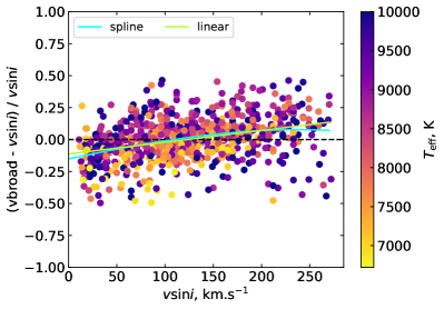
In order to distinguish evolutionary effects from rotational ones, we need reliable measurements of the stellar rotation. For this, we used the Gaia vbroad parameter, which is a measure of the total line broadening, hence is a projected quantity along the line of sight, like . In this subsection, we evaluate whether vbroad is a suitable substitute for .
The Gaia Team has already characterised the vbroad parameter available in DR3 in detail (Frémat et al., 2023). That study characterised vbroad for a range of stellar temperatures and brightnesses and explored the parameter’s technical details. Specifically, it examined behaviour either side of a temperature reference point of 7500 K, which happens to be near the middle of our range of interest. Here, we focus just on the A/F stars to estimate the reliability of vbroad for Sct pulsators.
The vbroad parameter is not a direct measurement of rotation, but rather all the line broadening present in the calcium triplet located within the 846–870 nm spectral range of the RVS spectrograph (Cropper et al., 2018; Frémat et al., 2023). As noted in Sec. 2, Sct stars are typically rapid rotators so rotation is expected to be the dominant contributor, but the instrumental broadening (, 26 km s-1) should not be forgotten. Micro- and macroturbulence should be insignificant for most Sct stars (Aerts et al., 2009; Landstreet et al., 2009; Doyle et al., 2014; Grassitelli et al., 2015) and, in any case, no macroturbulence is accounted for in the template spectra used in the vbroad calculation (Frémat et al., 2023). Especially for hot stars, the overall accuracy is sensitive to the quality of the match of those template spectra, and inaccuracies of 500 K in the template spectrum can have large detrimental effects on the resulting vbroad fit (see Frémat et al. 2023 for further details).666We note, therefore, that -derived temperatures would be insufficiently accurate for applications such as this.
We evaluated the Gaia vbroad measurements against a benchmark sample of rotational velocities for B/A/F stars (Zorec & Royer, 2012), catalogued from measurements made by Royer et al. (2007) wherein the details of their method for determining can be found. From this sample, we removed stars they had flagged as close binaries, so as not to bias results. We note that the Gaia team also removed vbroad measurements for stars detected as SB2s (Katz et al., 2023). After cross-matching the HD numbers from the Zorec & Royer (2012) catalogue with Gaia IDs with astroquery.simbad, we used astroquery.gaia to obtain phot_mean_g_mag, colour, ruwe, vbroad, and vbroad_error. We removed from the sample any stars without vbroad measurements. Since we are more interested in any systematic biases than in random errors, we also removed stars with fractional errors (vbroad_error/vbroad) greater than 10%. We note that too few stars had Gaia vsiniesphs for a useful comparison to be drawn, so our focus remained on vbroad.
Fig. 10 shows that vbroad tends to be 10–15% smaller than when the star is a slow rotator ( km s-1), performs well between 75 and 200 km s-1, but overestimates rotation velocities for rapid rotators ( km s-1). It also shows no strong temperature dependence, but the scatter is larger for stars near or above 10,000 K. The Sct instability strip blue edge lies at around 9000 K (Dupret et al., 2005; Xiong et al., 2016; Murphy et al., 2019), hence this should be unimportant for Sct stars generally. In conclusion, vbroad is a reliable indicator of rotation velocities for Sct stars, but underestimates the rotation velocity of slow rotators ( km s-1) by 10–15%.
5.3 The rotation distribution of stars in the ZAMS group
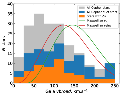
Having established that vbroad is sufficiently reliable, we consider the distribution of rotation velocities of stars in the ZAMS group of Cep–Her. We are interested in any dependence of pulsation properties on rotation velocity, so we defined three phenomenological groups: (i) the full ZAMS-group sample of Cep–Her stars; (ii) the subset of group (i) that pulsate; and (iii) the subset of group (ii) that have measurable . To limit mass-dependent effects on the vbroad distribution, we limit all three groups to the colour range where most pulsators are found, namely . We show their vbroad distribution in Fig. 11.
It appears that more rapid rotators are more likely to pulsate as Sct stars, consistent with the recent finding by Gootkin et al. (2024) who used an all-sky sample of TESS Scuti stars. We find it is possible to infer for approximately half of the Sct stars with vbroad 150 km s-1. Above this velocity, is only apparent for around 1 in 4. Hence, while more rapid rotators are more likely to pulsate, there is less order (regularity) to their mode frequencies.
Overall, the observed vbroad distribution of stars in CepHer is slower than expected from observations of field stars from Zorec & Royer (2012). An explanation for this is lacking – the systematic underestimation of by the vbroad parameter is only 10–15% and vanishes by km s-1 (Sec. 5.2), hence some other explanation is required.
5.4 The effect of rotation on pulsation
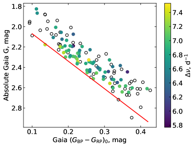
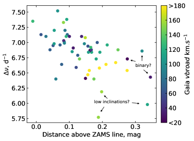
The values measured in Sec. 5.1 are tabulated in Table A and shown in Fig. 12 (top), wherein two trends are apparent. Firstly, stars with the lowest densities (lowest ) tend to lie farther above the ZAMS, as expected. We will attempt to separate the causes of those low densities shortly. Secondly, stars without a clear are preferentially those farther from the ZAMS line. We found that 40% of those are rapid rotators (vbroad in excess of 100 km s-1), confirming the oft-stated speculation that rapid rotation spoils the regular patterns (Sec. 3 and references therein).
Fig. 12 (bottom) shows that, as Gaia vbroad increases, the distance above the ZAMS line generally increases and generally decreases. There are a few noteworthy exceptions. Three stars at the bottom of the diagram, having the lowest , lie far above the ZAMS yet have only moderately high vbroad. These stars are TIC 17372709, TIC 158216795, and TIC 171884646. They are probably rapid rotators that are seen at low or moderate inclinations. There are also three stars on the right, lying particularly far above the ZAMS line, with moderate and low vbroad (TIC 27978717, TIC 135412676, and TIC 322497193 with vbroad = 22, 97, and 31 km s-1, respectively). They are unlikely to be rapid rotators seen at low inclination because they do not lie towards the bottom of the diagram (lower density). The obvious explanation is a binary companion that would cause these stars to appear brighter without being less dense. Hence, even with relatively simple asteroseismic data () we can infer when stars are rapid rotators seen pole on, and can potentially flag binaries that might be missed in other data (e.g. Gaia ruwe).
6 Summary
We have studied the Sct stars in the Cep–Her association to compare its pulsator fraction to that of associations or clusters of different ages, to evaluate the scaling relation on a statistically significant homogenous sample, and to study the interplay between pulsation and rotation. We collated stellar properties from Gaia and from the TESS Input Catalogue, and found that there is a subsample of Cep–Her stars that form a tight pack (‘the ZAMS group’) in a colour-magnitude diagram. That subsample should be free of large metallicity or age variations, and we analysed its stars in detail.
We employed four different methods to measure , thereby minimising any methodological (systematic) bias in the measurements. We found a correlation between dereddened Gaia colour and , whether examined as the range of measured values for each star, or as their mean. However, we found substantial scatter in that relation of 372 K at , even after an extensive outlier removal effort. This scatter is much larger (1000 K) if we do not exclude outliers or restrict our sample to the ZAMS group. Given that the instability strip is 2000 K wide, we surmise that the relation is of little practical use.
Nonetheless, by combining measurements from multiple clusters we observed some structure in the – diagram. Specifically, we found two ridges that bear similarity to those in the Period–luminosity diagram. A closer analysis of Gaia vbroad values along the ridges suggests (though only at 1) that rapid rotation causes stars to pulsate in lower radial orders, explaining the temperature-independent ridge of the young stars comprising our sample.
The pulsator fraction in Cep–Her peaks at 100%, at = 0.30–0.35 mag, corresponding to K. This is the first such measurement for an association or cluster younger than 100 Myr, and forms part of a continuing effort to better characterise the fraction of stars in the instability strip that pulsate. That effort began with Kepler and has continued with clusters of different ages observed by TESS. The emerging trend is that the pulsator fraction is higher for younger Sct stars, which we attribute to the onset of helium settling in young main-sequence A stars even before 100 Myr.
We evaluated the Gaia vbroad parameter against for an independent sample of A stars and concluded that vbroad is a reliable estimator of rotation velocities for Sct stars generally, but underestimates the rotation velocities of slow rotators ( km s-1) by 10–15%. We found that more rapid rotators in the instability strip are more likely to pulsate as Sct stars, albeit with less regular pulsation patterns, and that Cep–Her contains an unexplained excess of slow rotators.
We were able to measure the asteroseismic large spacing, , for 70 of the 126 stars in the ZAMS group via the échelle method. We observed that the pulsators for which could not be measured were preferentially the stars farthest from the ZAMS (i.e. stars of the lowest density). At least 40% of these were rapid rotators (high vbroad), hence our conclusion that rapid rotation does indeed spoil the regular patterns of modes in Sct stars. We also showed that a correlation between and rotation (via the proxy quantity ‘distance above the ZAMS’ in magnitudes), allows rapid rotators seen at low inclinations to be distinguished from slow rotators, and may assist with the identification of unresolved binaries.
Future work will include mode identification and the application of rotating models to determine asteroseismic ages for different subgroups in the Cep–Her Complex. Spectroscopic observations are ongoing, which will offer a narrow metallicity prior to hone the results. We expect to apply hierarchical Bayesian modelling to a dozen or so members of the Complex in this manner, refining both relative and absolute ages of the subgroups of Cep–Her.
Acknowledgements
We thank Daniel Foreman-Mackey for expanding on his numpyro tutorial and helping to apply it to the data analysed in Fig. 6. SJM was supported by the Australian Research Council (ARC) through Future Fellowship FT210100485. TRB was also supported by the ARC, through DP210103119 and FL220100117.
Software
Data Availability
We make our stellar parameters table (Table A) available online as a csv file accompanying this article. The table of the five strongest pulsation peaks (Table 4) is similarly available as a csv, and we provide a separate repository of all peaks (not just the first five) for each star. TESS data are publicly available online via the Mikulski Archive for Space Telescopes (MAST), and are readily accessible via the lightkurve package.
References
- Aerts et al. (2009) Aerts C., Puls J., Godart M., Dupret M.-A., 2009, A&A, 508, 409
- Aerts et al. (2010) Aerts C., Christensen-Dalsgaard J., Kurtz D. W., 2010, Asteroseismology. Springer-Verlag, Berlin
- Aerts et al. (2019) Aerts C., Mathis S., Rogers T. M., 2019, ARA&A, 57, 35
- Antoci et al. (2011) Antoci V., et al., 2011, Nature, 477, 570
- Antoci et al. (2014) Antoci V., et al., 2014, ApJ, 796, 118
- Astropy Collaboration et al. (2022) Astropy Collaboration et al., 2022, ApJ, 935, 167
- Baglin et al. (1973) Baglin A., Breger M., Chevalier C., Hauck B., Le Contel J. M., Sareyan J. P., Valtier J. C., 1973, A&A, 23, 221
- Bailer-Jones et al. (2021) Bailer-Jones C. A. L., Rybizki J., Fouesneau M., Demleitner M., Andrae R., 2021, AJ, 161, 147
- Bailyn (1995) Bailyn C. D., 1995, ARA&A, 33, 133
- Barac et al. (2022) Barac N., Bedding T. R., Murphy S. J., Hey D. R., 2022, MNRAS, 516, 2080
- Barbara et al. (2022) Barbara N. H., Bedding T. R., Fulcher B. D., Murphy S. J., Van Reeth T., 2022, MNRAS, 514, 2793
- Barceló Forteza et al. (2018) Barceló Forteza S., Roca Cortés T., García R. A., 2018, A&A, 614, A46
- Barceló Forteza et al. (2020) Barceló Forteza S., Moya A., Barrado D., Solano E., Martín-Ruiz S., Suárez J. C., García Hernández A., 2020, A&A, 638, A59
- Bastian & Lardo (2018) Bastian N., Lardo C., 2018, ARA&A, 56, 83
- Basu et al. (2011) Basu S., et al., 2011, ApJ, 729, L10
- Bedding & Kjeldsen (2022) Bedding T. R., Kjeldsen H., 2022, Research Notes of the American Astronomical Society, 6, 202
- Bedding et al. (2020) Bedding T. R., et al., 2020, Nature, 581, 147
- Bedding et al. (2023) Bedding T. R., et al., 2023, ApJ, 946, L10
- Bell (2020) Bell K. J., 2020, Research Notes of the American Astronomical Society, 4, 19
- Belokurov et al. (2020) Belokurov V., et al., 2020, MNRAS, 496, 1922
- Bingham et al. (2019) Bingham E., et al., 2019, J. Mach. Learn. Res., 20, 28:1
- Bouma et al. (2023) Bouma L. G., Palumbo E. K., Hillenbrand L. A., 2023, ApJ, 947, L3
- Bowman & Kurtz (2018) Bowman D. M., Kurtz D. W., 2018, MNRAS, 476, 3169
- Bowman et al. (2016) Bowman D. M., Kurtz D. W., Breger M., Murphy S. J., Holdsworth D. L., 2016, MNRAS, 460, 1970
- Bradbury et al. (2018) Bradbury J., et al., 2018, JAX: composable transformations of Python+NumPy programs, http://github.com/google/jax
- Breger (2000) Breger M., 2000, in M. Breger & M. Montgomery ed., Astronomical Society of the Pacific Conference Series Vol. 210, Delta Scuti and Related Stars. pp 3–+
- Breger & Bregman (1975) Breger M., Bregman J. N., 1975, ApJ, 200, 343
- Brogaard et al. (2016) Brogaard K., et al., 2016, Astronomische Nachrichten, 337, 793
- Brogaard et al. (2021) Brogaard K., Arentoft T., Jessen-Hansen J., Miglio A., 2021, MNRAS, 507, 496
- Brogaard et al. (2023) Brogaard K., et al., 2023, A&A, 679, A23
- Brown et al. (1991) Brown T. M., Gilliland R. L., Noyes R. W., Ramsey L. W., 1991, ApJ, 368, 599
- Casagrande et al. (2014) Casagrande L., et al., 2014, MNRAS, 439, 2060
- Chaplin & Miglio (2013) Chaplin W. J., Miglio A., 2013, ARA&A, 51, 353
- Christensen-Dalsgaard (2000) Christensen-Dalsgaard J., 2000, in Breger M., Montgomery M., eds, Astronomical Society of the Pacific Conference Series Vol. 210, Delta Scuti and Related Stars. p. 187
- Coelho et al. (2015) Coelho H. R., Chaplin W. J., Basu S., Serenelli A., Miglio A., Reese D. R., 2015, MNRAS, 451, 3011
- Cropper et al. (2018) Cropper M., et al., 2018, A&A, 616, A5
- Cunha et al. (2013) Cunha M. S., Alentiev D., Brandão I. M., Perraut K., 2013, MNRAS, 436, 1639
- Deal et al. (2016) Deal M., Richard O., Vauclair S., 2016, A&A, 589, A140
- Deal et al. (2020) Deal M., Goupil M. J., Marques J. P., Reese D. R., Lebreton Y., 2020, A&A, 633, A23
- Dornan & Lovekin (2022) Dornan V., Lovekin C. C., 2022, ApJ, 924, 130
- Doyle et al. (2014) Doyle A. P., Davies G. R., Smalley B., Chaplin W. J., Elsworth Y., 2014, MNRAS, 444, 3592
- Dupret et al. (2005) Dupret M., Grigahcène A., Garrido R., Gabriel M., Scuflaire R., 2005, A&A, 435, 927
- Dziembowski (1997) Dziembowski W., 1997, in Provost J., Schmider F.-X., eds, Vol. 181, Sounding Solar and Stellar Interiors. p. ISBN0792348389
- Evans (2018) Evans D. F., 2018, Research Notes of the American Astronomical Society, 2, 20
- Fitton et al. (2022) Fitton S., Tofflemire B. M., Kraus A. L., 2022, Research Notes of the American Astronomical Society, 6, 18
- Folsom et al. (2012) Folsom C. P., Bagnulo S., Wade G. A., Alecian E., Landstreet J. D., Marsden S. C., Waite I. A., 2012, MNRAS, 422, 2072
- Fossati et al. (2007) Fossati L., Bagnulo S., Monier R., Khan S. A., Kochukhov O., Landstreet J., Wade G., Weiss W., 2007, A&A, 476, 911
- Frémat et al. (2023) Frémat Y., et al., 2023, A&A, 674, A8
- Fujii et al. (2012) Fujii M. S., Saitoh T. R., Portegies Zwart S. F., 2012, ApJ, 753, 85
- Gaia Collaboration et al. (2023) Gaia Collaboration et al., 2023, A&A, 674, A1
- Gallenne et al. (2023) Gallenne A., Mérand A., Kervella P., Graczyk D., Pietrzyński G., Gieren W., Pilecki B., 2023, A&A, 672, A119
- Ginsburg et al. (2019) Ginsburg A., et al., 2019, AJ, 157, 98
- Gootkin et al. (2024) Gootkin K., Hon M., Huber D., Hey D. R., Bedding T. R., Murphy S. J., 2024, arXiv e-prints, p. arXiv:2405.19388
- Grassitelli et al. (2015) Grassitelli L., Fossati L., Langer N., Miglio A., Istrate A. G., Sanyal D., 2015, A&A, 584, L2
- Gray & Corbally (2002) Gray R. O., Corbally C. J., 2002, AJ, 124, 989
- Guzik (2021) Guzik J. A., 2021, Frontiers in Astronomy and Space Sciences, 8, 55
- Hasanzadeh et al. (2021) Hasanzadeh A., Safari H., Ghasemi H., 2021, MNRAS, 505, 1476
- Hekker (2020) Hekker S., 2020, Frontiers in Astronomy and Space Sciences, 7, 3
- Herczeg & Hillenbrand (2015) Herczeg G. J., Hillenbrand L. A., 2015, ApJ, 808, 23
- Heyl et al. (2022) Heyl J., Caiazzo I., Richer H. B., 2022, ApJ, 926, 132
- Hidalgo et al. (2018) Hidalgo S. L., et al., 2018, ApJ, 856, 125
- Houdek (2000) Houdek G., 2000, in Breger M., Montgomery M., eds, Astronomical Society of the Pacific Conference Series Vol. 210, Delta Scuti and Related Stars. p. 454
- Howell et al. (2024) Howell M., Campbell S. W., Stello D., De Silva G. M., 2024, MNRAS, 527, 7974
- Hunt & Reffert (2023) Hunt E. L., Reffert S., 2023, A&A, 673, A114
- Jenkins et al. (2016) Jenkins J. M., et al., 2016, in Proc. SPIE. p. 99133E, doi:10.1117/12.2233418
- Jeon et al. (2004) Jeon Y.-B., Lee M. G., Kim S.-L., Lee H., 2004, AJ, 128, 287
- Kahraman Aliçavuş et al. (2020) Kahraman Aliçavuş F., Poretti E., Catanzaro G., Smalley B., Niemczura E., Rainer M., Handler G., 2020, MNRAS, 493, 4518
- Kama et al. (2015) Kama M., Folsom C. P., Pinilla P., 2015, A&A, 582, L10
- Katz et al. (2023) Katz D., et al., 2023, A&A, 674, A5
- Kerr et al. (2022a) Kerr R., Kraus A. L., Murphy S. J., Krolikowski D. M., Offner S. S. R., Tofflemire B. M., Rizzuto A. C., 2022a, ApJ, 941, 49
- Kerr et al. (2022b) Kerr R., Kraus A. L., Murphy S. J., Krolikowski D. M., Bedding T. R., Rizzuto A. C., 2022b, ApJ, 941, 143
- Kerr et al. (2023) Kerr R., Kraus A. L., Rizzuto A. C., 2023, ApJ, 954, 134
- Kerr et al. (tted) Kerr R., Kraus A. L., Krolikowski D., Bouma L., submitted, ApJ
- Khan et al. (2023) Khan S., et al., 2023, A&A, 677, A21
- Kjeldsen & Bedding (1995) Kjeldsen H., Bedding T. R., 1995, A&A, 293, 87
- Kjeldsen et al. (2005) Kjeldsen H., et al., 2005, ApJ, 635, 1281
- Kjeldsen et al. (2008) Kjeldsen H., et al., 2008, ApJ, 682, 1370
- Kumar et al. (2019) Kumar R., Carroll C., Hartikainen A., Martin O., 2019, Journal of Open Source Software, 4, 1143
- Lallement et al. (2019) Lallement R., Babusiaux C., Vergely J. L., Katz D., Arenou F., Valette B., Hottier C., Capitanio L., 2019, A&A, 625, A135
- Landstreet et al. (2009) Landstreet J. D., Kupka F., Ford H. A., Officer T., Sigut T. A. A., Silaj J., Strasser S., Townshend A., 2009, A&A, 503, 973
- Lee (2021) Lee J. W., 2021, PASJ, 73, 809
- Li et al. (2021) Li Y., Bedding T. R., Stello D., Sharma S., Huber D., Murphy S. J., 2021, MNRAS, 501, 3162
- Li et al. (2023) Li G., et al., 2023, arXiv e-prints, p. arXiv:2311.16991
- Lightkurve Collaboration et al. (2018) Lightkurve Collaboration et al., 2018, Lightkurve: Kepler and TESS time series analysis in Python, Astrophysics Source Code Library (ascl:1812.013)
- Lignières & Georgeot (2009) Lignières F., Georgeot B., 2009, A&A, 500, 1173
- Lomb (1976) Lomb N. R., 1976, Ap&SS, 39, 447
- Lu et al. (2023) Lu Y., Angus R., Foreman-Mackey D., Hattori S., 2023, arXiv e-prints, p. arXiv:2310.14990
- Lyttle et al. (2021) Lyttle A. J., et al., 2021, MNRAS, 505, 2427
- McNamara (2011) McNamara D. H., 2011, AJ, 142, 110
- Michaud et al. (1983) Michaud G., Tarasick D., Charland Y., Pelletier C., 1983, ApJ, 269, 239
- Michel et al. (2017) Michel E., et al., 2017, in European Physical Journal Web of Conferences. p. 03001 (arXiv:1705.03721), doi:10.1051/epjconf/201716003001
- Miller et al. (2020) Miller N. J., Maxted P. F. L., Smalley B., 2020, MNRAS, 497, 2899
- Miller et al. (2022) Miller N. J., Maxted P. F. L., Graczyk D., Tan T. G., Southworth J., 2022, MNRAS, 517, 5129
- Murphy & Paunzen (2017) Murphy S. J., Paunzen E., 2017, MNRAS, 466, 546
- Murphy et al. (2014) Murphy S. J., Bedding T. R., Shibahashi H., Kurtz D. W., Kjeldsen H., 2014, MNRAS, 441, 2515
- Murphy et al. (2019) Murphy S. J., Hey D., Van Reeth T., Bedding T. R., 2019, MNRAS, 485, 2380
- Murphy et al. (2020a) Murphy S. J., Paunzen E., Bedding T. R., Walczak P., Huber D., 2020a, MNRAS, 495, 1888
- Murphy et al. (2020b) Murphy S. J., Saio H., Takada-Hidai M., Kurtz D. W., Shibahashi H., Takata M., Hey D. R., 2020b, MNRAS, 498, 4272
- Murphy et al. (2021) Murphy S. J., Joyce M., Bedding T. R., White T. R., Kama M., 2021, MNRAS, 502, 1633
- Murphy et al. (2022) Murphy S. J., Bedding T. R., White T. R., Li Y., Hey D., Reese D., Joyce M., 2022, MNRAS, 511, 5718
- Murphy et al. (2023) Murphy S. J., Bedding T. R., Gautam A., Joyce M., 2023, MNRAS,
- Niemczura et al. (2017) Niemczura E., et al., 2017, MNRAS, 470, 2870
- Olivares et al. (2018) Olivares J., et al., 2018, A&A, 617, A15
- Palla & Stahler (2000) Palla F., Stahler S. W., 2000, ApJ, 540, 255
- Pamos Ortega et al. (2022) Pamos Ortega D., García Hernández A., Suárez J. C., Pascual Granado J., Barceló Forteza S., Rodón J. R., 2022, MNRAS, 513, 374
- Pamos Ortega et al. (2023) Pamos Ortega D., Mirouh G. M., García Hernández A., Suárez Yanes J. C., Barceló Forteza S., 2023, A&A, 675, A167
- Pamyatnykh (2000) Pamyatnykh A. A., 2000, in Breger M., Montgomery M., eds, Astronomical Society of the Pacific Conference Series Vol. 210, Delta Scuti and Related Stars. p. 215 (arXiv:astro-ph/0005276)
- Pang et al. (2022) Pang X., et al., 2022, ApJ, 931, 156
- Paparó et al. (2016) Paparó M., Benkő J. M., Hareter M., Guzik J. A., 2016, ApJS, 224, 41
- Penoyre et al. (2022) Penoyre Z., Belokurov V., Evans N. W., 2022, MNRAS, 513, 5270
- Pérez Hernández et al. (1999) Pérez Hernández F., Claret A., Hernández M. M., Michel E., 1999, A&A, 346, 586
- Phan et al. (2019) Phan D., Pradhan N., Jankowiak M., 2019, arXiv preprint arXiv:1912.11554
- Poretti et al. (2008) Poretti E., et al., 2008, ApJ, 685, 947
- Pych et al. (2001) Pych W., Kaluzny J., Krzeminski W., Schwarzenberg-Czerny A., Thompson I. B., 2001, A&A, 367, 148
- Ramón-Ballesta et al. (2021) Ramón-Ballesta A., García Hernández A., Suárez J. C., Rodón J. R., Pascual-Granado J., Garrido R., 2021, MNRAS, 505, 6217
- Read et al. (2024) Read A. K., et al., 2024, MNRAS, 528, 2464
- Reese et al. (2017) Reese D. R., Lignières F., Ballot J., Dupret M.-A., Barban C., van’t Veer-Menneret C., MacGregor K. B., 2017, A&A, 601, A130
- Ricker et al. (2015) Ricker G. R., et al., 2015, Journal of Astronomical Telescopes, Instruments, and Systems, 1, 014003
- Rizzuto et al. (2018) Rizzuto A. C., Vanderburg A., Mann A. W., Kraus A. L., Dressing C. D., Agüeros M. A., Douglas S. T., Krolikowski D. M., 2018, AJ, 156, 195
- Royer et al. (2007) Royer F., Zorec J., Gómez A. E., 2007, A&A, 463, 671
- Saio (2005) Saio H., 2005, MNRAS, 360, 1022
- Sandquist et al. (2020) Sandquist E. L., et al., 2020, AJ, 159, 96
- Scargle (1982) Scargle J. D., 1982, ApJ, 263, 835
- Scutt et al. (2023) Scutt O. J., Murphy S. J., Nielsen M. B., Davies G. R., Bedding T. R., Lyttle A. J., 2023, MNRAS, 525, 5235
- Smalley et al. (2014) Smalley B., et al., 2014, A&A, 564, A69
- Smalley et al. (2017) Smalley B., et al., 2017, MNRAS, 465, 2662
- Sreenivas et al. (2024) Sreenivas K. R., Bedding T. R., Li Y., Huber D., Crawford C. L., Stello D., Yu J., 2024, MNRAS, 530, 3477
- Stassun & Torres (2021) Stassun K. G., Torres G., 2021, ApJ, 907, L33
- Stassun et al. (2019) Stassun K. G., et al., 2019, AJ, 158, 138
- Stȩpień (2000) Stȩpień K., 2000, A&A, 353, 227
- Stȩpień et al. (2017) Stȩpień K., Pamyatnykh A. A., Rozyczka M., 2017, A&A, 597, A87
- Steindl et al. (2022) Steindl T., Zwintz K., Müllner M., 2022, A&A, 664, A32
- Stello et al. (2009) Stello D., Chaplin W. J., Basu S., Elsworth Y., Bedding T. R., 2009, MNRAS, 400, L80
- Suárez et al. (2014) Suárez J. C., García Hernández A., Moya A., Rodrigo C., Solano E., Garrido R., Rodón J. R., 2014, A&A, 563, A7
- Tailo et al. (2022) Tailo M., et al., 2022, A&A, 662, L7
- Taylor (2022) Taylor J., 2022, Introduction to Error Analysis, the Study of Uncertainties in Physical Measurements, 3rd Edition. University Science Books; Melville, NY
- Templeton et al. (2002) Templeton M., Basu S., Demarque P., 2002, ApJ, 576, 963
- Theado & Cunha (2006) Theado S., Cunha M., 2006, Communications in Asteroseismology, 147, 101
- Théado et al. (2005) Théado S., Vauclair S., Cunha M. S., 2005, A&A, 443, 627
- Théado et al. (2009) Théado S., Vauclair S., Alecian G., Le Blanc F., 2009, ApJ, 704, 1262
- Titus & Morgan (1940) Titus J., Morgan W. W., 1940, ApJ, 92, 256
- Uzundag et al. (2023) Uzundag M., et al., 2023, MNRAS, 526, 2846
- White et al. (2018) White T. R., et al., 2018, MNRAS, 477, 4403
- Xiong et al. (2016) Xiong D. R., Deng L., Zhang C., Wang K., 2016, MNRAS, 457, 3163
- Yu et al. (2018) Yu J., Huber D., Bedding T. R., Stello D., Hon M., Murphy S. J., Khanna S., 2018, ApJS, 236, 42
- Ziaali et al. (2019) Ziaali E., Bedding T. R., Murphy S. J., Van Reeth T., Hey D. R., 2019, MNRAS, 486, 4348
- Zinn et al. (2018) Zinn J. C., Pinsonneault M. H., Huber D., Stello D., 2018, preprint, (arXiv:1805.02650)
- Zorec & Royer (2012) Zorec J., Royer F., 2012, A&A, 537, A120
- den Hartogh et al. (2020) den Hartogh J. W., Eggenberger P., Deheuvels S., 2020, A&A, 634, L16
Appendix A Data Tables
| (moment) | (smooth) | |||||||||||||||||
|---|---|---|---|---|---|---|---|---|---|---|---|---|---|---|---|---|---|---|
| TIC | HD | cadence | vert | e_ | ruwe | vbroad | e_vbroad | Amax | amp. | pow. | amp. | pow. | ||||||
| min | mag | mag | mag | mag | K | K | km s-1 | km s-1 | d-1 | ppt | d-1 | d-1 | d-1 | d-1 | d-1 | |||
| 7992735 | 348886 | 10 | 10.266 | 2.61 | 0.40 | 0.26 | 7163 | 174 | 0.99 | 26.04 | 4.35 | 19.27 | 1.091 | 18.91 | 19.37 | 18.24 | 19.43 | – |
| 8598196 | 349008 | 10 | 10.502 | 2.61 | 0.36 | 0.15 | 7390 | 191 | 1.32 | 47.30 | 4.14 | 21.112 | 0.544 | 24.00 | 22.48 | 23.23 | 22.82 | – |
| 11218613 | 228591 | 2 | 10.216 | 2.35 | 0.23 | 0.06 | 8085 | 188 | 1.01 | 102.08 | 20.25 | 35.672 | 1.275 | 49.21 | 46.49 | 50.49 | 45.81 | 7.52 |
| 11588737 | 228700 | 10 | 9.690 | 1.88 | 0.14 | 0.29 | 8673 | 206 | 1.29 | 194.54 | 14.39 | 32.819 | 4.574 | 26.20 | 31.52 | 28.53 | 32.03 | – |
| 11708996 | 228681 | 2 | 9.926 | 2.18 | 0.18 | 0.10 | 8356 | 123 | 0.82 | 154.88 | 12.89 | 44.398 | 2.144 | 38.41 | 45.08 | 45.40 | 46.31 | – |
| 12361752 | 228838 | 2 | 10.068 | 2.29 | 0.23 | 0.13 | 8031 | 155 | 0.87 | 145.81 | 14.02 | 44.871 | 1.216 | 44.15 | 44.82 | 44.58 | 44.86 | 6.73 |
| 13876477 | 229189 | 10 | 10.016 | 2.16 | 0.21 | 0.22 | 8038 | 139 | 0.92 | 282.78 | 19.20 | 22.112 | 1.318 | 23.26 | 22.09 | 23.31 | 21.57 | – |
| 15247229 | – | 2 | 9.997 | 2.18 | 0.18 | 0.10 | 8263 | 157 | 1.10 | 105.01 | 8.18 | 49.984 | 1.272 | 49.71 | 49.63 | 49.78 | 49.74 | – |
| 15478761 | – | 10 | 10.501 | 2.67 | 0.36 | 0.11 | 7397 | 158 | 1.10 | 22.94 | 5.91 | 19.29 | 0.126 | 16.83 | 17.18 | 16.28 | 21.67 | – |
| 16310676 | – | 10 | 9.633 | 1.95 | 0.09 | 0.10 | 8683 | 123 | 1.92 | 39.06 | 3.77 | 43.399 | 0.248 | 38.47 | 41.59 | 38.85 | 43.07 | – |
| 16621585 | – | 2 | 10.455 | 2.64 | 0.32 | 0.04 | 7552 | 147 | 0.94 | 46.25 | 9.40 | 27.964 | 0.775 | 25.30 | 25.55 | 24.93 | 25.58 | – |
| 16622862 | – | 2 | 10.494 | 2.72 | 0.34 | 0.00 | 7568 | 136 | 1.14 | 45.10 | 5.41 | 23.185 | 0.685 | 17.26 | 14.72 | 16.15 | 14.02 | – |
| 16739247 | – | 2 | 10.358 | 2.56 | 0.31 | 0.09 | 7706 | 178 | 0.99 | 115.74 | 14.11 | 22.909 | 1.563 | 28.79 | 26.93 | 28.16 | 26.95 | 7.38 |
| 17372709 | – | 2 | 10.040 | 2.19 | 0.21 | 0.19 | 8189 | 198 | 0.90 | 154.14 | 9.60 | 18.286 | 0.903 | 28.55 | 25.94 | 27.46 | 25.44 | 5.77 |
| 20774645 | – | 10 | 10.217 | 2.56 | 0.37 | 0.24 | 7356 | 134 | 1.01 | – | – | 28.404 | 0.11 | 24.17 | 25.30 | 10.00 | 34.92 | – |
| 20819550 | – | 2 | 10.508 | 2.45 | 0.25 | 0.03 | 7865 | 131 | 1.12 | 83.78 | 11.09 | 41.615 | 0.764 | 44.20 | 42.66 | 43.01 | 42.15 | 7.10 |
| 21150042 | – | 2 | 10.679 | 2.60 | 0.32 | 0.07 | 7584 | 143 | 0.87 | 68.31 | 8.42 | 22.508 | 1.061 | 27.84 | 25.12 | 26.92 | 25.36 | – |
| 27978717 | – | 10 | 9.846 | 1.83 | 0.11 | 0.28 | 8545 | 136 | 1.16 | 22.30 | 4.31 | 39.521 | 0.46 | 33.69 | 35.68 | 36.43 | 38.06 | 6.73 |
| 28397009 | – | 2 | 10.082 | 2.59 | 0.34 | 0.14 | 7490 | 126 | 1.23 | 36.34 | 3.45 | 21.595 | 1.129 | 28.60 | 25.70 | 26.96 | 24.38 | 7.10 |
| 28400691 | – | 10 | 10.355 | 2.53 | 0.38 | 0.31 | 7338 | 135 | 6.03 | 85.81 | 10.68 | 21.825 | 0.359 | 21.50 | 21.67 | 21.10 | 22.88 | – |
| 28679106 | – | 2 | 9.708 | 2.35 | 0.23 | 0.05 | 8094 | 145 | 1.06 | 109.90 | 7.08 | 50.842 | 1.584 | 52.57 | 53.32 | 53.06 | 53.70 | 7.20 |
| 29539591 | – | 10 | 9.896 | 2.01 | 0.21 | 0.35 | 8231 | 169 | 2.41 | 155.85 | 19.72 | 52.032 | 0.464 | 53.88 | 53.43 | 54.27 | 52.96 | – |
| 40485583 | 227470 | 2 | 9.770 | 1.95 | 0.14 | 0.24 | 8538 | 177 | 0.94 | – | – | 62.558 | 0.075 | 63.21 | 62.34 | 62.02 | 57.27 | – |
| 43795649 | – | 2 | 9.726 | 2.30 | 0.22 | 0.09 | 7839 | 129 | 0.98 | – | – | 38.535 | 1.094 | 33.90 | 34.90 | 35.07 | 35.61 | 7.07 |
| 63819901 | – | 2 | 10.183 | 2.50 | 0.26 | 0.01 | 8508 | 160 | 1.05 | 107.99 | 14.15 | 21.154 | 1.593 | 33.03 | 29.38 | 31.34 | 26.70 | – |
| 64050903 | – | 2 | 10.161 | 2.43 | 0.25 | 0.05 | 8599 | 351 | 1.04 | 64.04 | 5.52 | 50.16 | 0.42 | 41.59 | 43.28 | 15.82 | 14.12 | 6.95 |
| 66585916 | – | 2 | 9.945 | 2.24 | 0.19 | 0.08 | 8753 | 326 | 0.98 | 98.66 | 7.98 | 52.829 | 1.047 | 50.00 | 50.90 | 50.39 | 51.24 | 7.01 |
| 68757401 | – | 10 | 10.278 | 2.61 | 0.39 | 0.24 | 7199 | 129 | 3.54 | 238.96 | 15.02 | 21.767 | 0.126 | 24.43 | 24.16 | 22.85 | 28.88 | – |
| 68766561 | – | 2 | 9.598 | 2.26 | 0.20 | 0.08 | 8125 | 135 | 1.95 | 131.72 | 10.28 | 53.134 | 1.497 | 49.97 | 51.73 | 51.39 | 52.66 | – |
| 91212494 | 227853 | 2 | 10.069 | 2.45 | 0.30 | 0.17 | 7662 | 141 | 0.94 | 117.32 | 6.01 | 34.528 | 0.799 | 30.16 | 30.68 | 30.40 | 31.74 | 6.84 |
| 91825479 | 228034 | 2 | 9.702 | 2.07 | 0.21 | 0.30 | 8887 | 464 | 1.79 | – | – | 43.884 | 1.181 | 44.00 | 43.86 | 44.18 | 44.05 | 6.31 |
| 92428258 | 228216 | 2 | 9.613 | 2.01 | 0.17 | 0.24 | 8653 | 361 | 0.97 | – | – | 38.679 | 1.705 | 33.45 | 34.23 | 33.23 | 35.12 | 6.85 |
| 111560278 | – | 10 | 10.354 | 2.66 | 0.39 | 0.20 | 7271 | 332 | 0.95 | 57.35 | 6.24 | 23.301 | 0.738 | 28.22 | 28.95 | 31.65 | 29.87 | – |
| 120257786 | – | 2 | 10.090 | 2.35 | 0.27 | 0.18 | 7899 | 141 | 1.39 | 115.64 | 9.52 | 31.584 | 0.762 | 41.67 | 40.03 | 41.05 | 39.91 | 6.73 |
| 120361047 | – | 2 | 10.358 | 2.52 | 0.35 | 0.21 | 7469 | 122 | 1.06 | 240.67 | 9.07 | 29.878 | 0.593 | 28.65 | 27.14 | 27.31 | 27.15 | 6.64 |
| 120824631 | – | 10 | 10.295 | 2.64 | 0.37 | 0.15 | 7500 | 137 | 0.98 | 95.51 | 8.66 | 24.499 | 0.473 | 22.88 | 23.46 | 23.45 | 24.22 | 6.98 |
| 120827848 | – | 2 | 9.889 | 2.12 | 0.18 | 0.17 | 8274 | 151 | 1.00 | – | – | 48.041 | 1.585 | 46.20 | 47.48 | 47.20 | 47.64 | 6.42 |
| 121275246 | – | 2 | 10.193 | 2.44 | 0.26 | 0.06 | 8036 | 147 | 0.93 | 88.94 | 8.71 | 33.269 | 1.009 | 39.30 | 36.85 | 38.38 | 36.25 | 6.40 |
| 121537103 | – | 2 | 10.004 | 2.27 | 0.23 | 0.15 | 8106 | 136 | 0.84 | 105.50 | 6.01 | 48.192 | 0.821 | 44.84 | 45.92 | 45.83 | 46.74 | – |
| 121869336 | – | 2 | 10.316 | 2.35 | 0.26 | 0.16 | 7963 | 152 | 1.01 | 61.51 | 6.33 | 45.211 | 1.562 | 34.90 | 39.14 | 36.36 | 40.39 | 6.94 |
| TIC | ||||||||||
|---|---|---|---|---|---|---|---|---|---|---|
| d-1 | d-1 | d-1 | d-1 | d-1 | ppt | ppt | ppt | ppt | ppt | |