Backstepping Control of a Bicopter with Unknown Mass and Inertia

Globally Asymptotically Stable Adaptive Control of a
Bicopter with Unknown Mass and Inertia

Estimation inversion-free Adaptive Control of a
Bicopter with Unknown Mass and Inertia

Singularity-free Backstepping-based Adaptive Control of a
Bicopter with Unknown Mass and Inertia

Abstract

The paper develops a singularity-free backstepping-based adaptive control for stabilizing and tracking the trajectory of a bicopter system. In the bicopter system, the inertial parameters parameterize the input map. Since the classical adaptive backstepping technique requires the inversion of the input map, which contains the estimate of parameter estimates, the stability of the closed-loop system cannot be guaranteed due to the inversion of parameter estimates. This paper proposes a novel technique to circumvent the inversion of parameter estimates in the control law. The resulting controller requires only the sign of the unknown parameters. The proposed controller is validated in simulation for a smooth and nonsmooth trajectory-tracking problem.

keywords: adaptive backstepping control, dynamic extension, bicopter, multicopter.

I INTRODUCTION

Multicopters are extensively used in applications like precision agriculture [1], environmental surveys [2, 3], construction management [4], and load transportation [5]. Their growing popularity drives interest in enhancing their capabilities, but reliable control remains challenging due to nonlinear, time-varying dynamics and uncertain environments.

Common control techniques for multicopters [6, 7, 8] depend on accurate model parameters, making them sensitive to uncertainties [9, 10]. Adaptive methods like model reference adaptive control [11, 12], L1 adaptive control [13], adaptive sliding mode control [14, 15, 16], and retrospective cost adaptive control [17, 18] address some of these issues, but often lack stability guarantees or require pre-existing controllers. Conventional control architectures decompose multicopter dynamics into separate translational and rotational loops [19], simplifying design but not guaranteeing closed-loop stability. These approaches rely on the time separation principle, where successive loops are designed to be faster than the preceding loops.

This paper develops an adaptive controller for fully coupled nonlinear dynamics using a bicopter system, a simplified multicopter retaining key nonlinear dynamics. In particular, we develop an adaptive backstepping controller [20], overcoming the non-invertibility of the input map via dynamic extension [21]. A bicopter is a multicopter constrained to a vertical plane and thus is modeled by a 6th-order nonlinear instead of a 12th-order nonlinear system. Despite the lower dimension of the state space, the 6th-order bicopter retains the complexities of the nonlinear dynamics of an unconstrained multicopter.

As shown in our previous work reported in [22], the classical backstepping technique can not be used due to the non-invertibility of the input map. In a bicopter system, the input map is a tall matrix, and thus, the non-invertibility is structural rather than due to rank deficiency at a few points in the state space. As shown in [22], a dynamic extension of the equations of motion overcomes the structural non-invertibility of the input map. However, the new input map is still parameterized by the unknown parameters.

Unlike existing methods [23, 24, 25, 26], which apply to the systems with uncertainties in the dynamics map, the proposed technique is developed for systems with uncertainties in the input map. In the proposed method, the requirement of inversion of the input map is relaxed to the knowledge of the sign of the unknown parameters. This requirement is often benign since the sign of unknown parameters is known due to their physical interpretation. For example, inertial properties such as mass and inertia, which may be unknown, are positive. The key contribution of this paper is thus the extension of the backstepping framework to design an adaptive controller for a system with uncertainty in the input map, its application to design a control law with stability guarantee for a bicopter system, and validation in simulation.

The paper is organized as follows. Section II presents the equations of motion of the bicopter system. Section III describes the adaptive backstepping procedure to design the adaptive controller for the bicopter. Section IV presents the results of numerical simulations to validate the adaptive controller. Finally, the paper concludes with a discussion of results and future research directions in section V.

II Problem formulation

We consider the bicopter system shown in Figure 1. The derivation of the equations of motion and their dynamic extension is described in more detail in [27].

Figure 1: Bicopter configuration considered in this paper. The bicopter is constrained to the $\hat{\imath}_{\rm A}-\hat{\jmath}_{\rm A}$ plane and rotates about the $\hat{k}_{\rm A}$ axis of the inertial frame $\rm F_{A}.$ Note that $\overset{\rightharpoonup}{r}_{{\rm c}/w}=r_{1}\hat{\imath}_{\rm A}+r_{2}\hat{\jmath}_{\rm A}.$

The dynamically extended equations of motion are

$$\dot{x}_{1} =x_{2},$$ (1)

$$\dot{x}_{2} =f_{2}(x_{1},x_{2})+g_{2}(x_{3})\theta_{1},$$ (2)

$$\dot{x}_{3} =x_{4},$$ (3)

$$\dot{x}_{4} =g_{4}(\theta)u,$$ (4)

where

$$x_{1}\stackrel{{\scriptstyle\triangle}}{{=}}\begin{bmatrix}r_{1}\\ r_{2}\end{bmatrix},x_{2}\stackrel{{\scriptstyle\triangle}}{{=}}\begin{bmatrix}\dot{r}_{1}\\ \dot{r}_{2}\end{bmatrix},x_{3}\stackrel{{\scriptstyle\triangle}}{{=}}\begin{bmatrix}F\\ \phi\end{bmatrix},x_{4}\stackrel{{\scriptstyle\triangle}}{{=}}\begin{bmatrix}\dot{F}\\ \dot{\phi}\end{bmatrix},$$ (5)

and

$$u\stackrel{{\scriptstyle\triangle}}{{=}}\begin{bmatrix}\ddot{F}\\ M\end{bmatrix},\theta\stackrel{{\scriptstyle\triangle}}{{=}}\begin{bmatrix}m^{-1}\\ J^{-1}\end{bmatrix}.$$ (6)

$r_{1}$ and $r_{2}$ are the horizontal and vertical positions of the center of mass of the bicopter, $\dot{r}_{1}$ and $\dot{r}_{2}$ are the corresponding velocities, $\phi$ is the roll angle of the bicopter, $\dot{\phi}$ is the angular velocity of the bicopter, $F$ and $M$ are the total force and the total moment applied to the bicopter, respectively, and $m$ and $J$ are the mass and the moment of inertia of the bicopter, respectively. The functions

$$f_{2}(x_{1},x_{2}) \stackrel{{\scriptstyle\triangle}}{{=}}\begin{bmatrix}0\\ -g\end{bmatrix},$$ (7)

$$g_{2}(x_{3}) \stackrel{{\scriptstyle\triangle}}{{=}}\begin{bmatrix}-\sin(x_{3,2})x_{3,1}\\ \cos(x_{3,2})x_{3,1}\end{bmatrix},$$ (8)

$$g_{4}(\theta) \stackrel{{\scriptstyle\triangle}}{{=}}\begin{bmatrix}0&\theta_{2}\\ 1&0\end{bmatrix}.$$ (9)

Note that the system (1)-(4) is in pure feedback form since $x_{3}$ appears non-affinely in (2). Finally, since $g_{4}(\theta)$ is invertible, the backstepping framework can be applied to design a stabilizing controller.

III Adaptive Backstepping Control

In this section, we develop an adaptive controller based on the backstepping framework to stabilize the bicopter system. Unlike the controller designed in [22], the proposed controller does not require inversion of the parameter estimates.

Let $\xi_{1}\stackrel{{\scriptstyle\triangle}}{{=}}\begin{bmatrix}r_{{\rm d}1}&r_{{\rm d}2}\end{bmatrix}^{\rm T}\in{\mathbb{R}}^{2}$ denote the desired trajectory and define the tracking error $e_{1}\stackrel{{\scriptstyle\triangle}}{{=}}x_{1}-\xi_{1}.$

III-A $e_{1}$ stabilization

Consider the function

$$V_{1} \stackrel{{\scriptstyle\triangle}}{{=}}\dfrac{1}{2}e_{1}^{\rm T}e_{1}.$$ (10)

Differentiating (10) and using (1) yields $\dot{V}_{1}=e_{1}^{\rm T}\dot{x}_{1}=e_{1}^{\rm T}x_{2}.$ Note that if $x_{2}=-k_{1}e_{1},$ where $k_{1}>0,$ then $\dot{V}_{1}<0.$ However, $x_{2}$ is not the control signal and thus cannot be chosen arbitrarily. Instead, following the backstepping process, we design a control law that yields the desired $x_{2}$ response, as follows.

Define $e_{2}\stackrel{{\scriptstyle\triangle}}{{=}}x_{2}-\xi_{2},$ where

$$\xi_{2}\stackrel{{\scriptstyle\triangle}}{{=}}-k_{1}e_{1},$$ (11)

and $k_{1}>0$. Then, differentiating (10) yields

$$\dot{V}_{1} =-k_{1}e_{1}^{\rm T}e_{1}+e_{2}^{\rm T}e_{1}.$$ (12)

III-B $e_{2}$ stabilization

Define $p_{1}\stackrel{{\scriptstyle\triangle}}{{=}}\theta_{1}^{-1}$ and consider the function

$$V_{2} \stackrel{{\scriptstyle\triangle}}{{=}}V_{1}+\dfrac{1}{2}e_{2}^{\rm T}e_{2}+\dfrac{1}{2}\gamma_{1}^{-1}|\theta_{1}|\left(\hat{p}_{1}-p_{1}\right)^{2},$$ (13)

where $\gamma_{1}>0$ and $\hat{p}_{1}$ is an estimate of $p_{1}$. Differentiating (13) and using (12) yields $\dot{V}_{2}=-k_{1}e_{1}^{\rm T}e_{1}+e_{2}^{\rm T}\left(e_{1}+f_{2}+g_{2}(x_{3})\theta_{1}+k_{1}x_{2}\right)+\gamma_{1}^{-1}|\theta_{1}|\left(\hat{p}_{1}-p_{1}\right)\dot{\hat{p}}_{1}.$ However, $g(x_{3})$ is not the control signal and thus can not be chosen arbitrarily. Instead, following the backstepping process, we design a control law that yields the desired $g(x_{3})$ response, as follows.

Define $e_{3}\stackrel{{\scriptstyle\triangle}}{{=}}g(x_{3})-\xi_{3},$ where

$$\xi_{3}\stackrel{{\scriptstyle\triangle}}{{=}}-\hat{p}_{1}\left(e_{1}+f_{2}+k_{1}x_{2}\right)-k_{2}\sigma(\theta_{1})e_{2},$$ (14)

$\sigma(\theta_{1})$ is the sign of $\theta_{1},$ and $k_{2}>0$. Consider the parameter update law

$$\dot{\hat{p}}_{1}=\gamma_{1}\sigma(\theta_{1})e_{2}^{\rm T}\left(e_{1}+f_{2}+k_{1}x_{2}\right).$$ (15)

Then, differentiating (13) yields

$$\dot{V}_{2} =-k_{1}e_{1}^{\rm T}e_{1}-k_{2}|\theta_{1}|e_{2}^{\rm T}e_{2}+e_{3}^{\rm T}e_{2}\theta_{1}.$$ (16)

III-C $e_{3}$ stabilization

Consider the function

$$V_{3} \stackrel{{\scriptstyle\triangle}}{{=}}V_{2}+\dfrac{1}{2}e_{3}^{\rm T}e_{3}.$$ (17)

Differentiating (17) and using (16) yields $\dot{V}_{2}=-k_{1}e_{1}^{\rm T}e_{1}-k_{2}|\theta_{1}|e_{2}^{\rm T}e_{2}+e_{3}^{\rm T}(\theta_{1}e_{2}+\dfrac{\partial g(x_{3})}{\partial x_{3}}x_{4}+\dot{\hat{p}}_{1}\left(e_{1}+f_{2}+k_{1}x_{2}\right)+\hat{p}_{1}\left(x_{2}+k_{1}f_{2}\right)+k_{2}\sigma(\theta_{1})\left(f_{2}+k_{1}x_{2}\right)+\left(k_{1}\hat{p}_{1}+k_{2}\sigma(\theta_{1})\right)g_{2}(x_{3})\theta_{1}).$ However, $x_{4}$ is not the control signal and thus can not be chosen arbitrarily. Instead, following the backstepping process, we design a control law that yields the desired $x_{4}$ response, as follows.

Define $e_{4}\stackrel{{\scriptstyle\triangle}}{{=}}x_{4}-\xi_{4},$ where

$$\xi_{4} \stackrel{{\scriptstyle\triangle}}{{=}}{\mathcal{G}}_{2}^{-1}\Big{[}\dot{\hat{p}}_{1}\left(e_{1}+f_{2}+k_{1}x_{2}\right)+\hat{p}_{1}\left(x_{2}+k_{1}f_{2}\right)$$

$$\quad+k_{2}\sigma(\theta_{1})\left(f_{2}+k_{1}x_{2}\right)$$

$$\quad+\left(e_{2}+\left(k_{1}\hat{p}_{1}+k_{2}\sigma(\theta_{1})\right)g_{2}(x_{3})\right)\hat{\theta}_{1}+k_{3}e_{3}\Big{]},$$ (18)

$k_{3}>0$ and

$${\mathcal{G}}_{2}\stackrel{{\scriptstyle\triangle}}{{=}}\frac{\partial g_{2}}{\partial x_{3}}=\begin{bmatrix}-\cos(x_{3,2})x_{3,1}&-\sin(x_{3,2})\\ -\sin(x_{3,2})x_{3,1}&\cos(x_{3,2})\end{bmatrix}.$$ (19)

Then, differentiating (17) yields

$$\dot{V}_{3} =-k_{1}e_{1}^{\rm T}e_{1}-k_{2}|\theta_{1}|e_{2}^{\rm T}e_{2}-k_{3}e_{3}^{\rm T}e_{3}$$

$$\quad+e_{4}^{\rm T}{\mathcal{G}}_{2}^{\rm T}e_{3}+(\theta_{1}-\hat{\theta}_{1})e_{3}^{\rm T}(e_{2}$$

$$\quad+\left(k_{1}\hat{p}_{1}+k_{2}\sigma(\theta_{1})\right)g_{2}(x_{3})).$$ (20)

III-D $e_{4}$ stabilization

Define $p_{2}\stackrel{{\scriptstyle\triangle}}{{=}}\theta_{2}^{-1}$ and consider the function

$$V_{4} \stackrel{{\scriptstyle\triangle}}{{=}}V_{3}+\dfrac{1}{2}e_{4}^{\rm T}e_{4}+\dfrac{1}{2}\gamma_{2}^{-1}|\theta_{2}|\left(\hat{p}_{2}-p_{2}\right)^{2}$$

$$\quad+\dfrac{1}{2}\alpha_{1}^{-1}(\theta_{1}-\hat{\theta}_{1})^{2}+\dfrac{1}{2}\alpha_{2}^{-1}(\theta_{1}-\hat{\vartheta}_{1})^{2},$$ (21)

where $\gamma_{2}>0$, $\alpha_{1}>0$, $\alpha_{2}>0,$ $\hat{p}_{2}$ is an estimate of $p_{2}$, and $\hat{\theta}_{1}$ and $\hat{\vartheta}_{1}$ are estimates of $\theta_{1}$.

Differentiating (21) yields

$$\dot{V}_{4} =-k_{1}e_{1}^{\rm T}e_{1}-k_{2}|\theta_{1}|e_{2}^{\rm T}e_{2}-k_{3}e_{3}^{\rm T}e_{3}+$$

$$\quad(\theta_{1}-\hat{\theta}_{1})e_{3}^{\rm T}(e_{2}+\left(k_{1}\hat{p}_{1}+k_{2}\sigma(\theta_{1})\right)g_{2}(x_{3}))-$$

$$\quad(\theta_{1}-\hat{\theta}_{1})e_{3}^{\rm T}\alpha_{1}^{-1}\dot{\hat{\theta}}_{1}+$$

$$\quad e_{4}^{\rm T}(g_{4}(\theta)u+\Sigma+\Psi\theta_{1})+$$

$$\quad\gamma_{2}^{-1}|\theta_{2}|\left(\hat{p}_{2}-p_{2}\right)\dot{\hat{p}}_{2}-\alpha_{2}^{-1}(\theta_{1}-\hat{\vartheta}_{1})\dot{\hat{\vartheta}}_{1},$$ (22)

where

$$\Sigma \stackrel{{\scriptstyle\triangle}}{{=}}d_{t}\text{inv}{\mathcal{G}}_{2}\Bigg{[}\dot{\hat{p}}_{1}\left(e_{1}+k_{1}x_{2}+f_{2}\right)$$

$$\quad+\hat{p}_{1}\left(x_{2}+k_{1}f_{2}\right)+k_{2}\sigma(\theta_{1})\left(f_{2}+k_{1}x_{2}\right)$$

$$\quad+\hat{\theta}_{1}\left(e_{2}+k_{1}\hat{p}_{1}g_{2}(x_{3})+k_{2}\sigma(\theta_{1})g_{2}(x_{3})\right)+k_{3}e_{3}\Bigg{]}$$

$$\quad+{\mathcal{G}}_{2}^{-1}\Bigg{[}\gamma_{1}\sigma(\theta_{1})\Big{[}\left(f_{2}^{\rm T}+k_{1}x_{2}^{\rm T}\right)\left(e_{1}+k_{1}x_{2}+f_{2}\right)$$

$$\quad+e_{2}^{\rm T}\left(x_{2}+k_{1}f_{2}\right)\Big{]}\left(e_{1}+k_{1}x_{2}+f_{2}\right)$$

$$\quad+2\dot{\hat{p}}_{1}\left(x_{2}+k_{1}f_{2}\right)$$

$$\quad+2\hat{p}_{1}f_{2}+k_{2}\sigma(\theta_{1})k_{1}f_{2}+\dot{\hat{\theta}}_{1}\Big{(}e_{2}+k_{1}\hat{p}_{1}g_{2}(x_{3})$$

$$\quad+k_{2}\sigma(\theta_{1})g_{2}(x_{3})\Big{)}+\hat{\theta}_{1}\Big{(}f_{2}+k_{1}x_{2}+k_{1}\hat{p}_{1}g_{2}(x_{3})$$

$$\quad+k_{1}\hat{p}_{1}{\mathcal{G}}_{2}x_{4}+k_{2}\sigma(\theta_{1}){\mathcal{G}}_{2}x_{4}\Big{)}$$

$$\quad+k_{3}\Big{(}{\mathcal{G}}_{2}x_{4}+\dot{\hat{p}}_{1}\left(e_{1}+k_{1}x_{2}+f_{2}\right)+\hat{p}_{1}\left(x_{2}+k_{1}f_{2}\right)$$

$$\quad+k_{2}\sigma(\theta_{1})\left(f_{2}+k_{1}x_{2}\right)\Big{)}\Bigg{]}\in{\mathbb{R}}^{2},$$ (23)

$$\Psi \stackrel{{\scriptstyle\triangle}}{{=}}{\mathcal{G}}_{2}^{-1}\Bigg{[}\gamma_{1}\sigma(\theta_{1})(g_{2}(x_{3})^{\rm T}\Phi)\Phi+\dot{\hat{p}}_{1}k_{1}g_{2}(x_{3})$$

$$\quad+\hat{p}_{1}g_{2}(x_{3})+k_{1}k_{2}\sigma(\theta_{1})g_{2}(x_{3})+\hat{\theta}_{1}g_{2}(x_{3})$$

$$\quad+k_{1}k_{3}\hat{p}_{1}g_{2}(x_{3})+k_{2}k_{3}\sigma(\theta_{1})g_{2}(x_{3})\Bigg{]}\in{\mathbb{R}}^{2},$$ (24)

$$\Phi \stackrel{{\scriptstyle\triangle}}{{=}}e_{1}+k_{1}x_{2}+f_{2}\in{\mathbb{R}}^{2}.$$ (25)

Finally, consider the control law

$$u =-\left[\begin{bmatrix}0&1\\ \hat{p}_{2}&0\end{bmatrix}(\Sigma+\Psi\hat{\vartheta}_{1})+k_{4}\begin{bmatrix}0&1\\ \sigma(\theta_{2})&0\end{bmatrix}e_{4}\right],$$ (26)

where $k_{4}>0$ and the parameters update laws

$$\dot{\hat{p}}_{2} =\gamma_{2}\sigma(\theta_{2})\begin{bmatrix}1&0\end{bmatrix}e_{4}\begin{bmatrix}1&0\end{bmatrix}(\Sigma+\Psi\hat{\vartheta}_{1}),$$ (27)

$$\dot{\hat{\theta}}_{1} =\alpha_{1}e_{3}^{\rm T}\left(e_{2}+k_{1}\hat{p}_{1}g_{2}(x_{3})+k_{2}\sigma(\theta_{1})g_{2}(x_{3})\right),$$ (28)

$$\dot{\hat{\vartheta}}_{1} =\alpha_{2}\Sigma^{\rm T}e_{4}.$$ (29)

Substituting the control law and the parameter update laws above in (22) yields

$$\dot{V}_{4} =-k_{1}e_{1}^{\rm T}e_{1}-k_{2}|\theta_{1}|e_{2}^{\rm T}e_{2}$$

$$\quad-k_{3}e_{3}^{\rm T}e_{3}-k_{4}e_{4}^{\rm T}\begin{bmatrix}|\theta_{2}|&0\\ 0&1\end{bmatrix}e_{4}\leq 0.$$ (30)

III-E Stability Analysis

The following theorem uses the Barbashin-Krasovskii-LaSalle invariance principle to establish the asymptotic stability of the origin in the closed-loop system (1), (2), (3), (4), (26).

Theorem 1.

Consider the system (1), (2), (3), (4), the controller (26), and the parameter update laws (15), (27), (28), (29), where $\gamma_{1},\gamma_{2},\alpha_{1},\alpha_{2},\alpha_{3},k_{1},k_{2},k_{3},k_{4}>0.$ Then, the equilibrium point $(e_{1},e_{2},e_{3},e_{4})=(0,0,0,0)$ is asymptotically stable.

Proof.

Consider the function (21). Note that, for all $e_{1},e_{2},e_{3},e_{4}\in{\mathbb{R}}^{2},$ it follows from (22) that $\dot{V}_{4}\leq 0.$ Let $\ell>0$ and define

$$\Omega \stackrel{{\scriptstyle\triangle}}{{=}}\left\{e_{1},e_{2},e_{3},e_{4}\in\mathbb{R}^{2},\hat{p}_{1},\hat{p}_{2},\hat{\theta}_{1},\hat{\vartheta}_{1}\in\mathbb{R}:V_{4}\leq\ell\right\}.$$

Note that $\Omega$ is a compact set. Furthermore, since $\dot{V}_{4}\leq 0$ and $V_{4}>0,$ $\Omega$ is a invariant set.

Next, define $E\subset\Omega$ such that $e_{1}=e_{2}=e_{3}=e_{4}=0.$ Since $\dot{V_{4}}=0$ if and only if at $e_{1}=e_{2}=e_{3}=e_{4}=0,$ it follows that $E$ is the largest positively invariant set such that $\dot{V}_{4}=0.$ It thus follows from the Barbashin-Krasovskii-LaSalles’s invariance principle [28, p. 129] that $(e_{1},e_{2},e_{3},e_{4})=(0,0,0,0)$ is asymptotically stable. ∎

Remark 1.

Note that the control (26) requires the existence of $\Sigma$ and $\Psi$, which implies that ${\mathcal{G}}_{2}$ must be non-singular. If $F\neq 0,$ which is reasonably expected during the system’s operation, ${\mathcal{G}}_{2}$ is nonsingular.

IV Numerical Simulation

In this section, we apply the adaptive backstepping controller developed in the previous section to the trajectory tracking problem. In particular, the adaptive controller is used to follow an elliptical and a second-order Hilbert curve-based trajectory. Note that the adaptive controller is given by (26) with the parameter update laws (15), (27), (28), and (29). The control architecture is shown in Figure 2 and the estimation architecture is shown in Figure 3.

Figure 2: Singularity-free adaptive control architecture.

Figure 3: Parameter estimation architecture.

To simulate the bicopter, we assume that the mass of the bicopter $m$ is $1\ \rm kg$ and its moment of inertia $J$ is $0.2$ $\rm kgm^{2}.$ In the controller, we set $k_{1}=1$, $k_{2}=5$, $k_{3}=10$, and $k_{4}=20.$ In the adaptation laws presented in Figure 3, we set the estimator gains $\gamma_{1}=\gamma_{2}=\alpha_{1}=\alpha_{2}=0.1$, and the initial estimates $\hat{\theta}_{1}(0)=\hat{\vartheta}_{1}(0)=\hat{p}_{1}(0)=\hat{p}_{2}(0)=0.$

IV-A Elliptical Trajectory

The bicopter is commanded to follow an elliptical trajectory given by

$$r_{{\rm d}1}(t) =5\cos(\psi)-5\cos(\psi)\cos(\omega t)-3\sin(\psi)\sin(\omega t),$$ (31)

$$r_{{\rm d}2}(t) =5\sin(\psi)-5\sin(\psi)\cos(\omega t)+3\cos(\psi)\sin(\omega t),$$ (32)

where $\psi=45~{}\rm{deg}$ and $\omega=0.1\ \rm rad/s^{-1}.$ Figure 4 shows the trajectory-tracking response of the bicopter, where the desired trajectory is shown in black dashes, and the output trajectory response is shown in blue. Figure 5 shows the position $r_{1},r_{2}$ response, the roll angle $\phi$ response of the bicopter and the control $u$ generated by the adaptive backstepping controller (26).

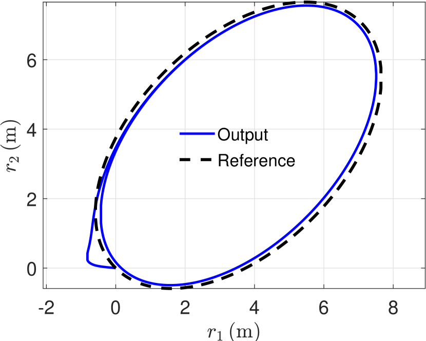
Figure 4: Elliptical trajectory. Tracking response of the bicopter with the adaptive backstepping controller. Note that the output trajectory is shown in solid blue, and the reference trajectory is in dashed black.

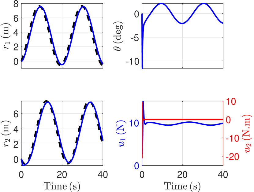
Figure 5: Elliptical trajectory. Position $(r_{1},r_{2})$, roll angle $\phi$ response and the input signal applied to the bicopter obtained with adaptive backstepping controller (26). Note that the references $r_{{\rm d}1},r_{{\rm d}2}$ is shown in black dashed lines

Figure 6 shows the estimates $\hat{\theta}_{1},\hat{\vartheta}_{1},$ and $\hat{p}_{1}$ of $\theta_{1}^{-1}$ and the estimate $\hat{p}_{2}$ of $\theta_{2}^{-1}.$ Note that the parameter estimates do not converge to their actual values. However, the non-convergence of the estimates is not due to persistency-related issues. In the adaptive controller design, since the parameter adaptation laws are chosen to cancel undesirable factors and not to estimate the parameters, the estimates do not necessarily need to converge.

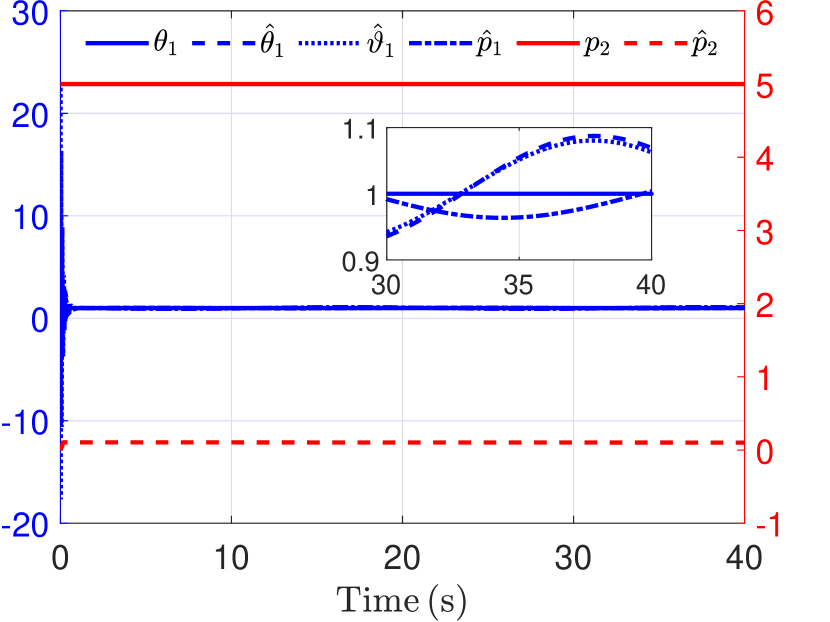
Figure 6: Elliptical trajectory. Estimates of $\theta_{1}$, $p_{1}=\theta_{1}^{-1}$, and $p_{2}=\theta_{2}^{-1}$ obtained with adaption laws (28), (29), (15), and (27).

Next, to improve the tracking performance, we increase the estimator gains by a factor of 10; that is, the gains are $\gamma_{1}=\gamma_{2}=\alpha_{1}=\alpha_{2}=1.$ Figures 7, 8, and 9 show the trajectory tracking response, input signals, and the parameter estimates with the larger estimator gains. Note that, although the trajectory tracking error improves, the required control effort also increases.

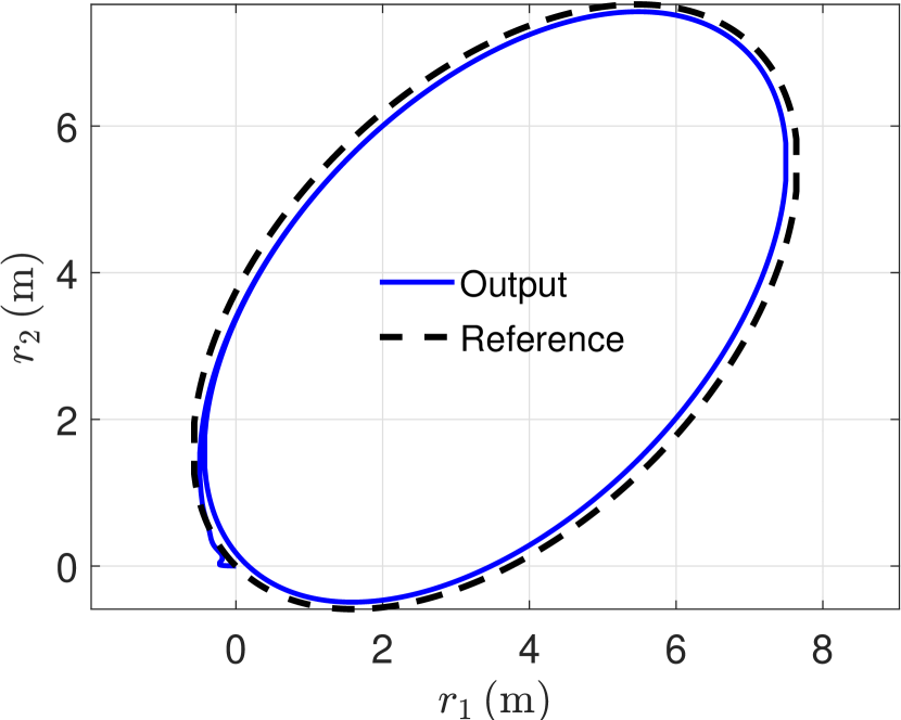
Figure 7: Elliptical trajectory. Tracking response of the bicopter with faster parameter estimation. Note that the output trajectory is shown in solid blue, and the reference trajectory is in dashed black.

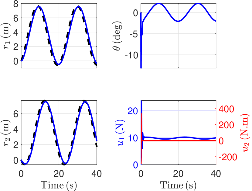
Figure 8: Elliptical trajectory. Position $(r_{1},r_{2})$ and roll angle $\phi$ response of the bicopter obtained with faster parameter estimation. Note that the references $r_{{\rm d}1},r_{{\rm d}2}$ is shown in black dashed lines

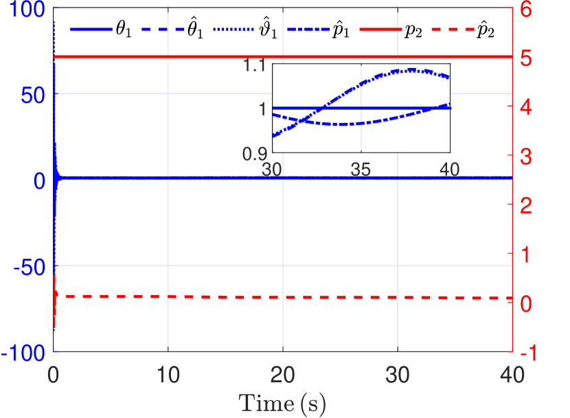
Figure 9: Elliptical trajectory. Estimates of $\theta_{1}$, $p_{1}=\theta_{1}^{-1}$, and $p_{2}=\theta_{2}^{-1}$ with larger parameter update gains

IV-B Hilbert trajectory

Next, the bicopter is commanded to follow a nonsmooth trajectory constructed using a second-order Hilbert curve. The trajectory is constructed using the algorithm described in Appendix A of [29] with a maximum velocity $v_{\rm max}=1\ \rm m/s$ and a maximum acceleration $a_{\rm max}=1\ \rm m/s^{2}.$ Figure 10 shows the trajectory-tracking response of the bicopter, where the desired trajectory is shown in black dashes, and the output trajectory response is shown in blue. Figure 11 shows the position $r_{1}$ and $r_{2}$ response, the roll angle $\phi$ response of the bicopter and the control $u$ generated by the adaptive backstepping controller (26).

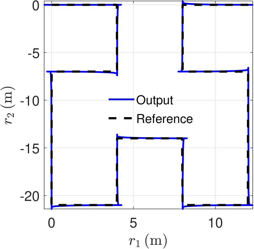
Figure 10: Hilbert trajectory. Tracking response of the bicopter with adaptive backstepping controller. Note that the output trajectory is in solid blue, and the desired trajectory is in dashed black.

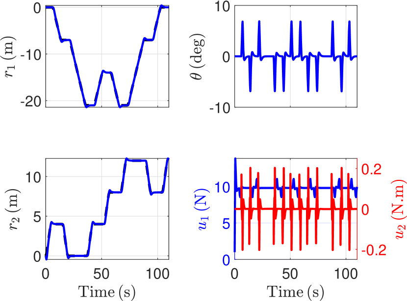
Figure 11: Hilbert trajectory. Positions $(r_{1},r_{2})$ and roll angle $\phi$ response of the bicopter with adaptive backstepping controller. Note that the references $r_{{\rm d}1},r_{{\rm d}2}$ is shown in black dashed lines

Figure 12 shows the estimates $\hat{\theta}_{1},\hat{\vartheta}_{1},$ and $\hat{p}_{1}$ of $\theta_{1}^{-1}$ and the estimate $\hat{p}_{2}$ of $\theta_{2}^{-1}.$ As in the previous case, note that the estimates do not converge to their actual values.

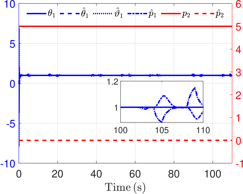
Figure 12: Hilbert trajectory. Estimates of $\theta_{1}$, $\theta_{1}^{-1}$, and $\theta_{2}^{-1}$ obtained with adaption laws (28), (29), (15), and (27).

Next, to improve the tracking performance, we increase the estimator gains by a factor of 10; that is, the gains are $\gamma_{1}=\gamma_{2}=\alpha_{1}=\alpha_{2}=1.$ Figures 13, 14, and 15 show the trajectory tracking response, input signals, and the parameter estimates with the larger estimator gains. Note that, although the trajectory tracking error improves, the required control effort also increases.

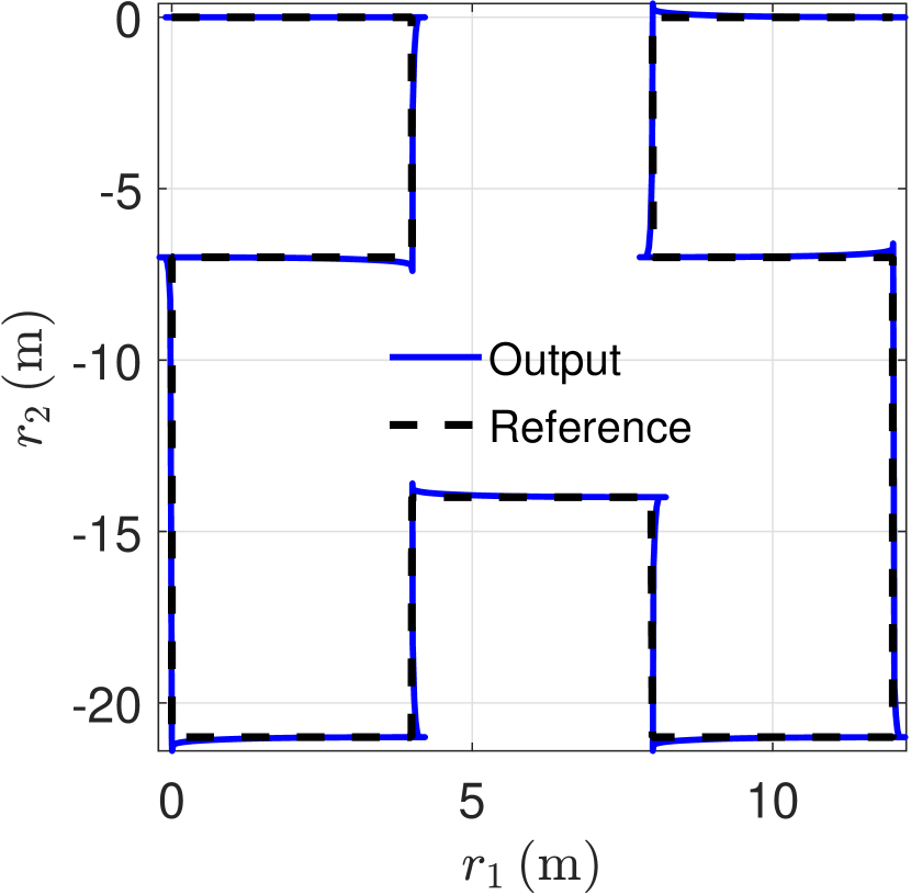
Figure 13: Hilbert trajectory. Tracking response of the bicopter with faster parameter estimation. Note that the output trajectory is shown in solid blue, and the reference trajectory is in dashed black.

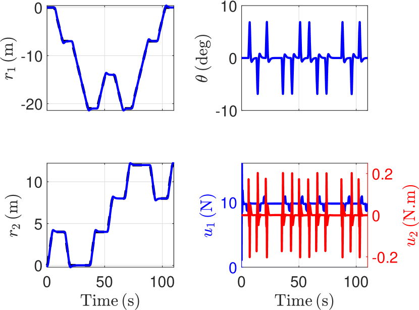
Figure 14: Hilbert trajectory. Position $(r_{1},r_{2})$ and roll angle $\phi$ response of the bicopter obtained with faster parameter estimation. Note that the references $r_{{\rm d}1},r_{{\rm d}2}$ is shown in black dashed lines

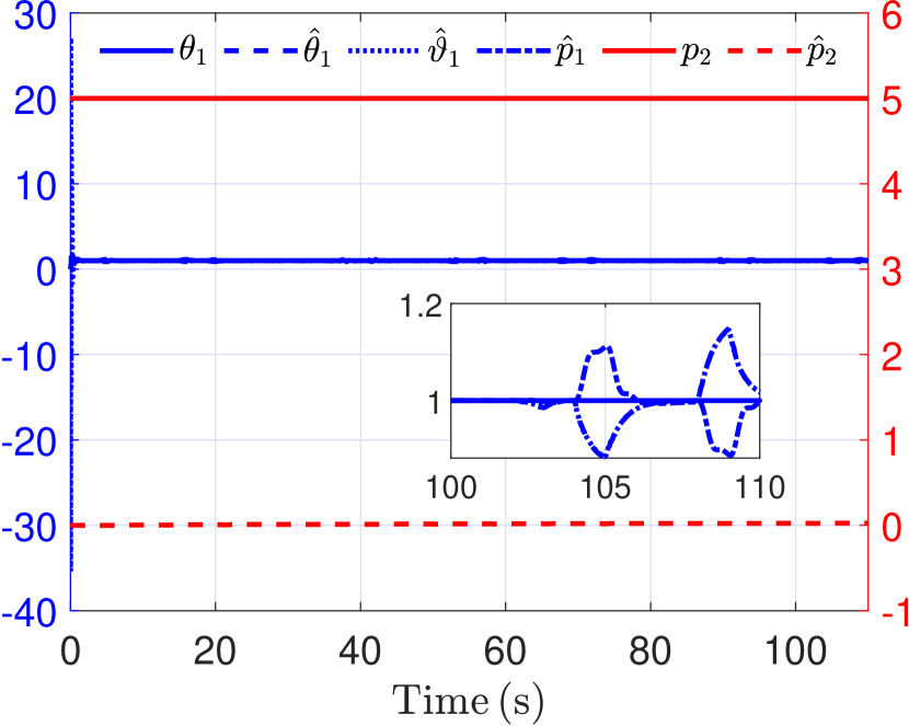
Figure 15: Hilbert trajectory. Estimates of $\theta_{1}$, $\theta_{1}^{-1}$, and $\theta_{2}$ with larger parameter update gains

V Conclusions

This paper presented an adaptive backstepping-based controller for the stabilization and tracking problem in a bicopter system. The adaptive controller and the parameter update laws are designed to circumvent the need to invert any system signal and only need the sign of the unknown mass and inertia, which are trivially known to be positive. The resulting closed-loop system is guaranteed to be stable and thus offers more flexibility in choosing gains to obtain any desired transient response. Numerical simulations show that the controller yields the desired tracking performance.

Future work will focus on extending the proposed technique to a full multicopter model. Furthermore, techniques to integrate state and control constraints to yield stronger performance guarantees will be investigated.

References

[1]Anandarup Mukherjee, Sudip Misra and Narendra Singh Raghuwanshi
“A survey of unmanned aerial sensing solutions in precision agriculture”
In J. Netw. Comput. Appl.148Elsevier, 2019, pp. 102461
[2]Arko Lucieer, Steven M de Jong and Darren Turner
“Mapping landslide displacements using Structure from Motion (SfM) and image correlation of multi-temporal UAV photography”
In Prog. Phys. Geogr.38.1Sage, 2014, pp. 97–116
[3]Victor V Klemas
“Coastal and environmental remote sensing from unmanned aerial vehicles: An overview”
In J. Coast. Res.31.5The Coastal EducationResearch Foundation, 2015, pp. 1260–1267
[4]Yan Li and Chunlu Liu
“Applications of multirotor drone technologies in construction management”
In Int. J. Constr. Manag.19.5Taylor & Francis, 2019, pp. 401–412
[5]Daniel KD Villa, Alexandre S Brandao and Mário Sarcinelli-Filho
“A survey on load transportation using multirotor UAVs”
In J. Intell. Robot. Syst.98Springer, 2020, pp. 267–296
[6]Tiago P Nascimento and Martin Saska
“Position and attitude control of multi-rotor aerial vehicles: A survey”
In Annu. Rev. Contr.48Elsevier, 2019, pp. 129–146
[7]Julius A Marshall, Wei Sun and Andrea L’Afflitto
“A survey of guidance, navigation, and control systems for autonomous multi-rotor small unmanned aerial systems”
In Annu. Rev. Contr.52Elsevier, 2021, pp. 390–427
[8]Pedro Castillo, Alejandro Dzul and Rogelio Lozano
“Real-time stabilization and tracking of a four-rotor mini rotorcraft”
In IEEE Trans. Contr. Sys. Tech.12.4IEEE, 2004, pp. 510–516
[9]Bara J Emran and Homayoun Najjaran
“A review of quadrotor: An underactuated mechanical system”
In Annu. Rev. Contr.46Elsevier, 2018, pp. 165–180
[10]Roohul Amin, Li Aijun and Shahaboddin Shamshirband
“A review of quadrotor UAV: control methodologies and performance evaluation”
In Int. J. Autom. Contr.10.2Inderscience Publishers (IEL), 2016, pp. 87–103
[11]Brian Whitehead and Stefan Bieniawski
“Model reference adaptive control of a quadrotor UAV”
In AIAA Guid. Nav. Contr. Conf. Ex., 2010, pp. 8148
[12]Zachary T Dydek, Anuradha M Annaswamy and Eugene Lavretsky
“Adaptive control of quadrotor UAVs: A design trade study with flight evaluations”
In IEEE Trans. Contr. Sys. Tech.21.4IEEE, 2012, pp. 1400–1406
[13]Zongyu Zuo and Pengkai Ru
“Augmented L1 adaptive tracking control of quad-rotor unmanned aircrafts”
In IEEE. Trans. Aerosp. Elec. Sys.50.4IEEE, 2014, pp. 3090–3101
[14]Tadeo Espinoza-Fraire et al.
“Trajectory tracking with adaptive robust control for quadrotor”
In Applied Sciences11.18MDPI, 2021, pp. 8571
[15]Zhuohuan Wu et al.
“L1 Adaptive Augmentation for Geometric Tracking Control of Quadrotors”
In 2022 International Conference on Robotics and Automation (ICRA), 2022, pp. 1329–1336
IEEE
[16]Omid Mofid and Saleh Mobayen
“Adaptive sliding mode control for finite-time stability of quad-rotor UAVs with parametric uncertainties”
In ISA trans.72Elsevier, 2018, pp. 1–14
[17]Ankit Goel et al.
“Experimental Implementation of an Adaptive Digital Autopilot”
In Proc. Amer. Contr. Conf., 2021, pp. 3737–3742
[18]John Spencer et al.
“An adaptive PID autotuner for multicopters with experimental results”
In Proc. Int. Conf. Rob. Autom., 2022, pp. 7846–7853
IEEE
[20]Miroslav Krstić, Petar V. Kokotović and Ioannis Kanellakopoulos
“Nonlinear and Adaptive Control Design”
John Wiley & Sons, 1995
[21]Jacques Descusse and Claude H Moog
“Decoupling with dynamic compensation for strong invertible affine non-linear systems”
In International Journal of Control42.6Taylor & Francis, 1985, pp. 1387–1398
[22]Jhon Manuel Portella Delgado, Mohammad Mirtaba and Ankit Goel
“Adaptive Backstepping Control of a Bicopter in Pure Feedback Form with Dynamic Extension”
In arXiv preprint arXiv:2402.03709, 2024
[23]Sheng Zhang and Wei-Qi Qian
“Dynamic backstepping control for pure-feedback nonlinear systems”
In Computing Research Repositoryabs/1706.08641, 2017
arXiv: http://arxiv.org/abs/1706.08641
[24]Frédéric Mazenc, Laurent Burlion and Michael Malisoff
“Backstepping Design for Output Feedback Stabilization for a Class of Uncertain Systems using Dynamic Extension”
In 2nd IFAC Conference on Modelling, Identification and Control of Nonlinear Systems, 2018, pp. 260–265
[25]Johann Reger and Lukas Triska
“Dynamic extensions for exact backstepping control of systems in pure feedback form”
In 58th IEEE Conference on Decision and Control, 2019, pp. 480–486
[26]Lukas Triska, Jhon Portella and Johann Reger
“Dynamic extension for adaptive backstepping control of uncertain pure-feedback systems”
In IFAC-PapersOnLine54.14Elsevier, 2021, pp. 307–312
[27]Jhon Manuel Portella Delgado, Mohammad Mirtaba and Ankit Goel
“Adaptive Backstepping Control of a Bicopter in Pure Feedback Form with Dynamic Extension”
In arXiv preprint arXiv:2402.03709, 2024
[28]Hassan K Khalil
“Nonlinear systems”
Prentice Hall, 2002
[29]John Spencer et al.
“An adaptive pid autotuner for multicopters with experimental results”
In 2022 International Conference on Robotics and Automation (ICRA), 2022, pp. 7846–7853
IEEE