Demons registration for 2D empirical wavelet transform: Application to texture segmentation

Demons registration for 2D empirical wavelet transform: Application to texture segmentation

Abstract

The empirical wavelet transform is a fully adaptive time-scale representation that has been widely used in the last decade. Inspired by the empirical mode decomposition, it consists of filter banks based on harmonic mode supports. Recently, it has been generalized to build the filter banks from any generating function using mappings. In practice, the harmonic mode supports can have low constrained shape in 2D, leading to numerical difficulties to compute the mappings and therefore the related wavelet filters. This work aims to propose an efficient numerical scheme to compute empirical wavelet coefficients using the demons registration algorithm. Results show that the proposed approach gives a numerically robust wavelet transform. An application to texture segmentation of scanning tunnelling microscope images is also presented.

Keywords: Empirical wavelet, adaptive representation, demons algorithm, texture segmentation.

1 Introduction

The empirical wavelet transform is a fully adaptive time-scale representation, introduced in [5], based on data-driven filter banks. Unlike the traditional wavelet transform, the wavelet filters are not designed on the basis of prescribed scales independent of the data under study, but on the basis of supports that contain the underlying harmonic modes. This approach is inspired by the empirical mode decomposition [13], but is based on solid theoretical foundations that the latter lacks. Due to its robust performance in decomposing images, it has led to many applications such as glaucoma detection [19, 21], hyperspectral image classification [20], cancer histopathological image classification [4], medical image fusion [23, 22] and texture segmentation [15]. Notably, it has been shown to outperform traditional wavelet transforms in extracting appropriate texture features from images [14, 16].

The last decade has seen an intensive development of the 2D empirical wavelet transform. The extraction of harmonic modes can be performed by scale-space representations [7] and several methods of separation of the harmonic modes in possibly low constrained shaped supports have been proposed, such as the Tensor [5], Ridgelet, Curvelet [16], Watershed [9] and Voronoi [6] methods. However, the design of filter banks has mainly long been limited to a specific generating function based on the Littlewood-Paley formulation. This formulation relies on a separable definition or the distance to the boundaries of the supports, which limits its extension to other generating functions. Recently, a general framework has been proposed to consider classic generating functions [18]. Deformations of a homogeneous or separable wavelet kernel are carried out by mappings between the data’s Fourier supports and the generating function’s Fourier support. In practice, this approach suffers from the difficulty to estimate the required mappings with constraints of invertibility, continuity and differentiability.

In this work, we propose a numerical implementation of the empirical wavelet transform based on the demons algorithm, widely used in image registration. We particularly compare different variants of the demons algorithm for the design of wavelet filters and the wavelet reconstruction from homogeneous and separable wavelet kernels. An application to the texture segmentation of scanning tunnelling microscope images is also considered for illustration. In Section 3, we recall the framework of empirical wavelet transform based on mappings, introduce specific band-pass wavelet filters and present different demons algorithms for mapping estimation. In Section 4, we compare numerically the mapping estimators for empirical wavelet transforms and show the application to texture segmentation. Finally, a discussion is provided in Section 5. A Matlab toolbox will be made publicly available at the time of publication.

2 Notations

We recall that an invertible function $\gamma$ is called a homeomorphism if it is continuous of inverse continuous and a diffeomorphism if it is infinitely differentiable of inverse infinitely differentiable. We consider that the space of square integrable functions $\mathrm{L}^{2}({\mathbb{R}}^{2})$ is endowed with the usual inner product

$$\langle f,g\rangle=\int_{{\mathbb{R}}^{2}}f(x)\overline{g(x)}\mathrm{d}x.$$

The Fourier transform $\widehat{f}$ of a function $f\in\mathrm{L}^{2}({\mathbb{R}}^{2})$ and its inverse are given by, respectively,

$$\widehat{f}(\xi)={\mathcal{F}}(f)(\xi)=\int_{{\mathbb{R}}^{2}}f(x)e^{-2\pi i(\xi\cdot x)}\mathrm{d}x,$$

$$f(x)={\mathcal{F}}^{-1}(\widehat{f})(x)=\int_{{\mathbb{R}}^{2}}\widehat{f}(\xi)e^{2\pi i(\xi\cdot x)}\mathrm{d}\xi,$$

where $\cdot$ stands for the dot product in ${\mathbb{R}}^{2}$.

3 Empirical wavelet transform

3.1 Empirical wavelet systems

The coonstruction of empirical wavelets relies on the partitioning of the Fourier domain $\Omega$. Technically, we consider a family of disjoint open sets $\{\Omega_{n}\}_{n\in\Upsilon}$, with $\Upsilon\subset{\mathbb{Z}}$, of closures $\overline{\Omega}_{n}$ covering the Fourier domain, i.e., $\Omega=\bigcup_{n\in\Upsilon}\overline{\Omega_{n}}$. In this work, we focus on real-valued images, which implies that the Fourier domain is symmetric, leading to consider a partition $\{\Omega_{n}\}_{n\in\Upsilon}$ that is symmetric, i.e., such that $\Omega_{-n}=\{-\xi\mid\xi\in\Omega_{n}\}$. To obtain such a partition, the modes of the Fourier spectrum are obtained by scale-space representation [7] and the Fourier domain is partitioned by the Watershed [16] or Voronoi [6] methods. Figure 1 shows an example of an image and the Watershed and Voronoi partitions of the logarithm of its Fourier spectrum using a scale-space step-size parameter set to $s_{0}=0.8$.

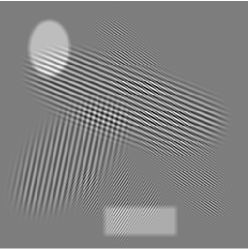
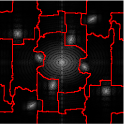
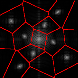
Figure 1: Fourier partitioning. Toy image of size $256\times 256$ along with the (middle) Watershed and (right) Voronoi partitions (overlapping in red) of the logarithm of their Fourier spectra.

Symmetric empirical wavelet systems are built as filters mostly supported on the sets $\Omega_{n}\cup\Omega_{-n}$ for $n\in\Upsilon^{+}=\{n\in\Upsilon\mid n\geq 0\}$ the subset of positive elements of $\Upsilon$. In [18], it has been proposed to build filters $\chi_{n}$ from a wavelet kernel $\psi$ using mappings $\gamma_{n}$ on ${\mathbb{R}}^{2}$. Let $\psi$ such that its Fourier trasnform $\widehat{\psi}$ is localized in frequency and compactly (or rapidly decaying) supported by a connected open subset $\Lambda$. Let $\gamma_{n}$ be mappings on ${\mathbb{R}}^{2}$ such that $\Lambda=\gamma_{n}(\Omega_{n})\textrm{ if }\Omega_{n}$ is bounded and $\Lambda\subsetneq\gamma_{n}(\Omega_{n})$ otherwise. Empirical wavelet systems $\psi_{n}$ and their symmetric counterparts $\chi_{n}$ are then defined as follows.

Definition 1 (Normalized empirical wavelet system).

Assume that the mappings $\gamma_{n}$ are diffeomorphisms. The symmetric empirical wavelet system $\{\chi_{n}\}_{n\in\Upsilon}$ corresponding to the partition $\{\Omega_{n}\}_{n\in\Upsilon}$ is defined by, for all $\xi\in{\mathbb{R}}^{2}$,

$$\widehat{\chi}_{0}(\xi)=\widehat{\psi}_{0}(\xi)\quad\textrm{ and }\quad\forall n\in\Upsilon\setminus\{0\},\quad\widehat{\chi}_{n}(\xi)=\frac{1}{\sqrt{2}}\left(\widehat{\psi}_{n}(\xi)+\widehat{\psi}_{-n}(\xi)\right),$$

where, for every $n\in\Upsilon$,

$$\widehat{\psi}_{n}(\xi)=\frac{1}{\sqrt{a_{n}(\xi)}}\;\widehat{\psi}\circ\gamma_{n}(\xi),\qquad\textrm{with }\quad a_{n}(\xi)=\frac{1}{|\mathrm{det}\;J_{\gamma_{n}}(\xi)|},$$

with $\gamma_{-n}:\xi\mapsto-\gamma_{n}(-\xi)$ and $J_{\gamma_{n}}$ being the Jacobian of the mapping $\gamma_{n}$.

The symmetry of the filter $\widehat{\chi}_{n}$ has to be understood with respect to the Fourier support $n$, i.e. $\widehat{\chi}_{n}=\widehat{\chi}_{-n}$. The normalization coefficient $a_{n}(\xi)$ ensures that

$$\int_{\Omega_{n}}|\widehat{\chi}_{n}(\xi)|^{2}\mathrm{d}\xi=\int_{\Lambda}|\widehat{\psi}(\xi)|^{2}\mathrm{d}\xi,$$ (1)

in most cases (see [18] for more details). If $\gamma_{n}$ is not a diffeomorphism, the substitution theorem ensuring the energy conservation (1) is not valid despite the use of the normalization coefficient $a_{n}(\xi)$. However, in practice, estimating diffeomorphisms is a difficult and computationally expensive task. Since an intervertible continuous function is a homeopmorphism if and only if it is an open map, i.e., a map for which the preimage of an open set is an open set, the existence of homeomorphisms is a milder assumption and their estimation is less difficult. We thus propose an unnormalized definition for the case when $\gamma_{n}$ is only a homeomorphism by removing the Jacobian determinant from Definition 1 as follows.

Definition 2 (Unnormalized empirical wavelet system).

Assume that the mapping $\gamma_{n}$ is a homeomorphism. The unnormalized symmetric empirical wavelet system $\{\chi_{n}\}_{n\in\Upsilon}$ corresponding to the partition $\{\Omega_{n}\}_{n\in\Upsilon}$ is defined by, for all $\xi\in{\mathbb{R}}^{2}$,

$$\widehat{\chi}_{0}(\xi)=\widehat{\psi}_{0}(\xi)\quad\textrm{ and }\quad\forall n\in\Upsilon\setminus\{0\},\quad\widehat{\chi}_{n}(\xi)=\widehat{\psi}_{n}(\xi)+\widehat{\psi}_{-n}(\xi),$$

where $\widehat{\psi}_{n}=\widehat{\psi}\circ\gamma_{n}$ and $\gamma_{-n}:\xi\mapsto-\gamma_{n}(-\xi)$.

The empirical wavelet transform consists of a filtering process from a normalized or unnormalized empirical wavelet system, as follows.

Definition 3 (Empirical wavelet transform).

The symmetric empirical wavelet transform is defined by, for all $n\in\Upsilon$,

$${\mathcal{E}}_{\chi}^{f}(\cdot,n)={\mathcal{F}}^{-1}\left(\widehat{f}.\overline{\widehat{\chi}_{n}}\right),$$

where ${\mathcal{F}}$ denotes the inverse Fourier transform.

Figure 2 shows an example of unnormalized wavelet filter’s Fourier transforms $\widehat{\chi}_{n}$ and the resulting wavelet coefficients ${\mathcal{E}}_{\chi}^{f}(\cdot,n)$ for the toy image in Figure 1 (left) and the Watershed partition of its Fourier spectrum given in Figure 1 (middle).

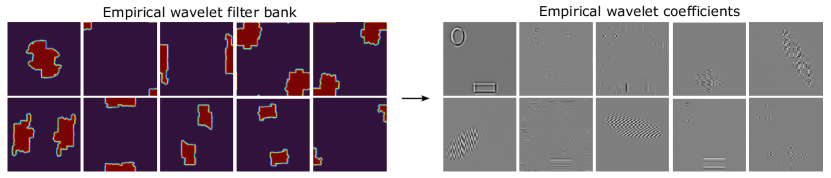
Figure 2: Empirical wavelet filtering. Example of unnormalized symmetric empirical wavelet filters $\chi_{n}$ in the Fourier domain (left) and resulting wavelet coefficients ${\mathcal{E}}_{\chi}^{f}(\cdot,n)$ (right), for $n=1,\ldots,10$, associated with the toy image using the Watershed partitioning.

The reconstruction of a real-valued image $f$ from its symmetric empirical wavelet transform ${\mathcal{E}}_{\chi}^{f}$ is guaranteed by Theorem 4.3 in [18], recalled hereafter.

Theorem 1 (Reconstruction).

Let $\Upsilon^{+}=\{n\in\Upsilon:n\geq 0\}$. Let assume that, for $a.e.\,\xi\in{\mathbb{R}}^{2}$, $0<\sum_{n\in\Upsilon^{+}}\left|\widehat{\psi}_{n}(\xi)\right|^{2}<\infty$ and $\sum_{n\in\Upsilon^{+}\setminus\{0\}}\left|\widehat{\psi}_{n}(\xi)\right|\left|\widehat{\psi}_{-n}(\xi)\right|<\infty.$ Then

$$f=\sum_{n\in\Upsilon^{+}}{\mathcal{E}}_{\chi}^{f}(\cdot,n)\star{\mathcal{F}}^{-1}\left(\frac{\widehat{\chi}_{n}}{\displaystyle\sum_{m\in\Upsilon^{+}}\left|\widehat{\chi}_{m}\right|^{2}}\right),$$ (2)

where $\star$ denotes the convolution of functions and ${\mathcal{F}}^{-1}$ denotes the inverse Fourier transform.

3.2 Band-pass empirical wavelets

For the study of the numerical behavior of the empirical wavelet transform, it is more convenient to consider band-pass filters. Therefore, we propose in this section to define homogeneous or separable 2D wavelet band-pass filters. The band-pass wavelet filters proposed in [16, 5] relie on the semi-Euclidean distance to the boundaries of the supports, which is equivalent to a discrete mapping. In 1D, this wavelet kernel can be adapted to the continuous framework as follows.

Definition 4 (1D band-pass wavelet).

The 1D band-pass wavelet, mostly supported by the segment $\Lambda=[-\frac{1}{2},\frac{1}{2}]$, is defined by, for every $\xi\in{\mathbb{R}}$,

$$\widehat{\psi}_{\tau}^{\rm 1D}(\xi)=\begin{cases}1&\textrm{if }|\xi|<\frac{1}{2}-\tau,\\ \displaystyle\cos\frac{\pi}{2}\beta\left(\frac{\tau-\frac{1}{2}+|\xi|}{2\tau}\right)&\textrm{if }\frac{1}{2}-\tau\leq|\xi|\leq\frac{1}{2}+\tau,\\ 0&\textrm{otherwise},\end{cases}$$

where $0<\tau<\frac{1}{2}$ is a transition width and $\beta$ is a continuous function on $[0,1]$ such that $\beta(0)=0$, $\beta(1)=1$ and $\beta(x)+\beta(1-x)=1$ for every $x\in[0,1]$.

The function $\beta$ is usually chosen as $\beta(x)=x^{4}(35-84x+70x^{2}-20x^{3})$. The 1D band-pass wavelet can be extended to 2D in a homogeneous or separable way, as proposed in the following definitions.

Definition 5 (Disk band-pass wavelet).

The disk band-pass wavelet, mostly supported by the disk $\Lambda=\mathrm{B}(0,\frac{1}{2})$, is defined by, for every $\xi\in{\mathbb{R}}^{2}$,

$$\widehat{\psi}^{\mathrm{D}}_{\tau}(\xi)=\begin{cases}1&\textrm{if }\|\xi\|_{2}<\frac{1}{2}-\tau,\\ \displaystyle\cos\frac{\pi}{2}\beta\left(\frac{\tau-\frac{1}{2}+\|\xi\|_{2}}{2\tau}\right)&\textrm{if }\frac{1}{2}-\tau\leq\|\xi\|_{2}\leq\frac{1}{2}+\tau,\\ 0&\textrm{otherwise},\end{cases}$$

where $0<\tau<\frac{1}{2}$ is a transition width and $\beta$ is a continuous function on $[0,1]$ such that $\beta(0)=0$, $\beta(1)=1$ and $\beta(x)+\beta(1-x)=1$ for every $x\in[0,1]$.

             

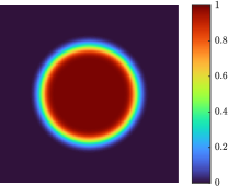
Figure 3: Band-pass wavelet. Disk (left) and square (right) band-pass wavelet with transition width $\tau=0.2$.

Definition 6 (Square band-pass wavelet).

The square band-pass wavelet, mostly supported by the square $\Lambda=[-\frac{1}{2},\frac{1}{2}]\times[-\frac{1}{2},\frac{1}{2}]$, is defined by, for every $\xi=(\xi_{1},\xi_{2})\in{\mathbb{R}}^{2}$,

$$\widehat{\psi}^{\mathrm{S}}_{\tau}(\xi)=\widehat{\psi}_{\tau}^{\rm 1D}(\xi_{1})\;\widehat{\psi}_{\tau}^{\rm 1D}(\xi_{2}),$$

where $0<\tau<\frac{1}{2}$ is a transition width.

Figure 3 show examples of disk and square band-pass wavelet filters.

Theorem 2.

Let $\chi^{\mathrm{D},\tau}_{n}=\chi^{\mathrm{D}}_{\tau}\circ\gamma_{n}$ and $\chi^{\mathrm{S},\tau}_{n}=\chi^{\mathrm{S}}_{\tau}\circ\gamma_{n}$ the (normalized or unnormalized) symmetric wavelet systems resulting from the disk and square band-pass wavelets $\widehat{\psi}_{\tau}^{D}$ and $\widehat{\psi}_{\tau}^{S}$, respectively, for every $n\in\Upsilon$. The reconstruction formula (2) holds for the normalized and unnormalized systems $\{\chi^{\mathrm{D},\tau}_{n}\}_{n\in\Upsilon}$ and $\{\chi^{\mathrm{S},\tau}_{n}\}_{n\in\Upsilon}$.

Proof.

Let $\widehat{\psi}_{\tau}$ be either $\widehat{\psi}_{\tau}=\widehat{\psi}_{\tau}^{D}$ or $\widehat{\psi}_{\tau}=\widehat{\psi}_{\tau}^{S}$. We set $\Lambda_{\tau}=\mathrm{B}(0,\frac{1}{2}+\tau)$ if $\widehat{\psi}_{\tau}=\widehat{\psi}_{\tau}^{D}$ and $\Lambda_{\tau}=[-\frac{1}{2}-\tau,\frac{1}{2}+\tau]\times[-\frac{1}{2}-\tau,\frac{1}{2}+\tau]$ if $\widehat{\psi}_{\tau}=\widehat{\psi}_{\tau}^{S}$. Let $\xi\in\Omega_{m}$. Since there exists a finite number of $\gamma_{n}$ such that $\gamma_{n}(\xi)\in\Lambda_{\tau}$, we have

$$\sum_{n\in\Upsilon^{+}}\left|\widehat{\psi}_{n}(\xi)\right|^{2}=\sum_{n\in\Upsilon^{+}}\left|\frac{1}{a_{n}(\xi)}\right|\left|\widehat{\psi}_{\tau}(\gamma_{n}(\xi))\right|^{2}=\sum_{n\in\Upsilon_{m}^{+}}\left|\frac{1}{a_{n}(\xi)}\right|\left|\widehat{\psi}_{\tau}(\gamma_{n}(\xi))\right|^{2}<+\infty,$$

where $\Upsilon_{m}^{+}=\{n\in\Upsilon^{+}:\gamma_{n}(\xi)\in\Lambda_{\tau}\}$ and $a_{n}(\xi)=1$ or $a_{n}(\xi)=1/|\mathrm{det}\;J_{\gamma_{n}}(\xi)|$ for the normalized or unnormalized empirical walet system, respectively. Moreover, since $\widehat{\psi}_{\tau}(\gamma_{m}(\xi))\neq 0$ and $a_{n}(\xi)>0$ for every $n\in\Upsilon$, we have $0<\sum_{n\in\Upsilon^{+}}|\widehat{\psi}_{n}(\xi)|^{2}$. Similarly, we can show that $\sum_{n\in\Upsilon^{+}}|\widehat{\psi}_{n}(\xi)\widehat{\psi}_{-n}(\xi)|<+\infty$. Hence the reconstruction formula (2) for $\{\chi^{\mathrm{D},\tau}_{n}\}_{n\in\Upsilon}$ and $\{\chi^{\mathrm{S},\tau}_{n}\}_{n\in\Upsilon}$ holds by Theorem 1. ∎

3.3 Mapping estimation

In practice, the mappings $\gamma_{n}$ in Definition LABEL:def:norm_system,def:unnorm_system have to be estimated. The Thirion’s demons algorithm [24] is a mapping estimation scheme inspired by a diffusion process in which the targeted mapping is represented by a displacement field $\gamma$. This method alternates between solving the flow equations and regularization. To give a theoretical justification to this method, [25] revisited it as the following optimisation problem:

$$\underset{\gamma,c\in{\mathcal{F}}({\mathbb{R}}^{2})}{\mathrm{minimize}}\quad\|\Lambda-\Omega\circ c\|_{2}^{2}+\frac{1}{\sigma_{x}^{2}}\|\gamma-c\|_{2}^{2}+\mathcal{R}(\gamma),$$ (3)

where $\Lambda$ and $\Omega$ are considered as functions from ${\mathbb{R}}^{2}$ to ${\mathbb{R}}$, ${\mathcal{F}}({\mathbb{R}}^{2})$ denotes the set of mappings on ${\mathbb{R}}^{2}$, $c$ is an intermediate mapping to account for noisy data, $\sigma_{x}$ controls the spatial uncertainty on the mappings and $\mathcal{R}(\gamma)$ is a regularization term.

The additive demons proposed in [3] consists of estimating the minimum $s$ of Equation 3 using an intermediate displacement field $u$ such that $c=\gamma+u$ and alternate

$$\displaystyle\underset{u\in{\mathcal{F}}({\mathbb{R}}^{2})}{\mathrm{minimize}}\quad\|\Lambda-\Omega\circ(\gamma+u)\|_{2}^{2}+\frac{1}{\sigma_{x}^{2}}\|u\|_{2}^{2}:=E(u),$$ (4)

$$\displaystyle\underset{\gamma\in{\mathcal{F}}({\mathbb{R}}^{2})}{\mathrm{minimize}}\quad\frac{1}{\sigma_{x}^{2}}\|\gamma-c\|_{2}^{2}+\mathcal{R}(\gamma).$$ (5)

The displacement field $u$ minimizing Equation 4 is approximated by, for every position $p\in R^{N}$,

$$u(p)\approx\frac{\Lambda(p)-\Omega\circ\gamma(p)}{\displaystyle\|\nabla(\Omega\circ\gamma)(p)\|_{2}^{2}-\frac{\sigma_{i}^{2}}{\sigma_{x}^{2}}|\Lambda(p)-\Omega\circ\gamma(p)|^{2}}\nabla\Omega^{\top},$$ (6)

where $\nabla$ denotes the gradient of functions. This implies that $\sigma_{x}$ controls the maximum step length: $\|u(p)\|_{2}\leq\sigma_{x}/2$ for every $p\in{\mathbb{R}}^{2}$. As for the minimization of Equation 5 with a regularization term $\mathcal{R}(\gamma)=\|\nabla\gamma\|_{2}^{2}/\sigma_{d}^{2}$, it corresponds to a convolution with a Gaussian kernel $G_{\rm diff}(\sigma_{d})$ of standard deviation $\sigma_{d}$. This regularization $\mathcal{R}(\gamma)$ has been modified by [3] in order to add a fluid-like regularization $G_{\rm fluid}(\sigma_{f})$ of standard deviation $\sigma_{f}$. To ensure the mapping $\gamma$ to be diffeomorphic, an alternative update of $c$ with an exponential field has been proposed in [25]: $c=s\circ\exp(u)$. The additive and diffeomorphic demons are summarized in Algotirhm 1.

1 Input: Sets $\Lambda$, $\Omega$.

2 Initialization: Displacement field $\gamma^{[0]}$.

3 $k=0$ ;

4 while $k\leq K$ and $|E(\gamma^{[k]})-E(\gamma^{[k-5]})|/E(\gamma^{[0]})>\epsilon$ do

5       $k\leftarrow k+1$ ;

6       Update $u^{[k]}$ from $\gamma^{[k-1]}$ using Equation 6 ;

7       Fluid-like regularization: $\gamma^{[k]}=G_{\rm fluid}(\sigma_{f})\star u^{[k]}$ ;

8       Either additive update $c^{[k]}=\gamma^{[k-1]}+u^{[k]}$

       or diffeomorphic update $c^{[k]}=\gamma^{[k-1]}\circ\exp(u^{[k]})$  ;

9       Diffusion-like regularization: $\gamma^{[k]}=G_{\rm diff}(\sigma_{d})\star c^{[k]}$ ;

10Output: Displacement field $\gamma^{[K]}$.

Algorithm 1 Vercauteren’s demons

For large deformations, a multiresolution scheme is necessary: the demons is performed iteratively from the lowest to the highest resolution. This scheme is summarized in Algotirhm 2.

1 Input: Sets $\Lambda$, $\Omega$.

2 Initialization: Displacement field $\gamma^{[0]}=\mathbf{0}$.

3 for $k=N_{\rm level},\ldots,1$ do

4       $\Lambda^{[k]},\Omega^{[k]},\gamma^{[k]}$ $\leftarrow$ Downsample $\Lambda$, $\Omega$ and $\gamma^{[k-1]}/2^{k}$ by $2^{k}$

5       $\gamma^{*}\leftarrow\textrm{Demons}(\Lambda^{[k]},\Omega^{[k]})$ initialized with $\gamma^{[k]}$     (Algotirhm 1)

6       $\gamma^{[k]}$ $\leftarrow$ Upsample $2^{k}\gamma^{*}$ by $2^{k}$

7Output: Displacement field $\gamma^{[N_{\rm level}]}$

Algorithm 2 Multiresolution demons

4 Numerical experiments

In this section, we compare the Thirion’s demons (Matlab function imregdemons) and the additive or diffeomorphic Vercauteren’s demons (Matlab toolbox available at https://www.mathworks.com/matlabcentral/fileexchange/39194-diffeomorphic-log-demons-image-registration) for the computation of estimates $\widetilde{\gamma}_{n}$ of the mappings $\gamma_{n}$. We consider the toy image and the sets $\Omega_{n}$ obtained by either Watershed or Voronoi partitioning presented in Figure 1.

4.1 Mapping estimation set-up

For the three demons, the diffusion-like parameter $\sigma_{d}$ and number of resolution levels $N_{\rm level}$ are selected by minimizing the quadratic risk $\|\Lambda-\Omega_{n}\circ\widetilde{\gamma}_{n}\|_{2}^{2}$ on the values $(\sigma_{d},N_{level})\in(0.3,0.31,\ldots,0.5)\times(n_{P}-1,n_{P})$, with $n_{P}$ the highest integer such that $2^{n_{P}}$ is smaller than each dimension of the image. For the Thirions’s demons, the numbers of iterations at the $N_{level}$ pyramid levels are set to $(2^{4},\ldots,2^{N_{level}+1})$ from the highest to the lowest pyramid level. For the Vercauteren’s demons, the maximum step length is set to $\sigma_{x}=5$, the fluid-like regularization is set to $\sigma_{f}=1$, the error threshold in the stop criterion is set to $\epsilon=10^{-3}$ and the maximum number of iterations is set to $K=500$.

4.2 Assessment measures

The accuracy of an estimate $\widetilde{\gamma}_{n}$ is measured using the Root Mean Squared Error defined as

$$\mathrm{RMSE}(\Lambda,\Omega_{n},\widetilde{\gamma}_{n})=\frac{1}{\sqrt{N_{\rm pixels}}}\|\Lambda-\Omega_{n}\circ\widetilde{\gamma}_{n}\|_{2},$$

where $N_{\rm pixels}$ is the number of pixels in the image $\Lambda$. The reconstruction $\widetilde{f}$ of the image $f$, with values in $[0,1]$, obtained by Equation 2 is assessed using the Peak Signal-to-Noise Ratio (PSNR) defined as

$$\mathrm{PSNR}(f,\widetilde{f})=-10\log_{10}\|\widetilde{f}-f\|_{2}^{2}.$$

4.3 Mapping estimation assessment

We assess the behavior of the different algorithms to map a partition to a generating function’s Fourier support which is usually a disk or a square. Table 1 reports the average RMSE of the estimated mappings $\widetilde{\gamma}_{n}$ from the sets $\Omega_{n}$ of the Watershed or Voronoi partition to the disk or square $\Lambda$ for the different demons algorithms. The additive and Thirion’s demons have similar average performance, but the additive one suffers from less variability, and both outperform the diffeomorphic demons due to the latter’s additional constraint on diffeomorphicity. In addition, the performance of all demons is better for the more shape-constrained Voronoi partition than for the Watershed partition, and better for the disk than for the square due to its irregularity.

Table 1: RMSE $\times 10^{-2}$ averaged over the sets $\Omega_{n}$ (with lowest and highest values) for the different demons algorithms, partitions $\{\Omega_{n}\}_{n\in\Upsilon}$ and sets $\Lambda$.

Demons	Watershed $\boldsymbol{\rightarrow}$ Disk	Watershed $\boldsymbol{\rightarrow}$ Square	Voronoi $\boldsymbol{\rightarrow}$ Disk	Voronoi $\boldsymbol{\rightarrow}$ Square
Thirion’s	$4.37\quad(0.82-18.43)$	$4.59\quad(0.31-20.03)$	$2.41\quad(0.58-13.71)$	$2.32\quad(0.32-6.80)$
Additive	$3.83\quad(2.13-5.13)$	$4.30\quad(2.47-7.23)$	$3.00\quad(2.14-4.17)$	$3.08\quad(2.23-4.14)$
Diffeomorphic	$5.64\quad(3.00-10.29)$	$7.35\quad(3.15-14.47)$	$4.03\quad(2.86-6.04)$	$6.41\quad(2.00-17.05)$

In addition, Table 2 reports the computtional time of the different demons algorithms for the Watershed and Voronoi partitions $\{\Omega_{n}\}_{n\in\Upsilon}$ and the disk and square sets $\Lambda$. The Thirion’s demons is the fastest algorithm and the diffeomorphic demons is much more computationally costly than the two other demons.

Table 2: Computational times ($h$:$min$:$sec$) of the demons algorithms for the different partitions $\{\Omega_{n}\}_{n\in\Upsilon}$ and sets $\Lambda$.

Demons	Watershed $\boldsymbol{\rightarrow}$ Disk	Watershed $\boldsymbol{\rightarrow}$ Square	Voronoi $\boldsymbol{\rightarrow}$ Disk	Voronoi $\boldsymbol{\rightarrow}$ Square
Thirion’s	$00:02:44$	$00:02:50$	$00:02:48$	$00:02:44$
Additive	$00:12:50$	$00:11:35$	$00:14:51$	$00:12:17$
Diffeomorphic	$01:43:22$	$01:32:25$	$01:27:53$	$01:44:40$

To assess the invertibility, continuity and diffeomorphicity of the mapping estimates, we explore the behavior of the resulting empirical wavelet coefficients expected to be concave and equal to one on most of each support $\Omega_{n}$. Figure 4 and Figure 5 show the disk band-pass empirical wavelet coefficients $\widehat{\chi}_{n}^{\mathrm{D},\tau}$, where $\tau=0.2$, with and without normalization, respectively, for the Watershed partition and the different demons algorithms. The normalized coefficients are not concave for the additive and Thirion’s demons due to the discontinuity of the normalization coefficient while they are concave but very sparse for the diffeomorphic demons. The unnormalized wavelet coefficients are more satisfactory as they are continuous, concave and mostly equal to one for each $\Omega_{n}$. However, the coefficients obtained using the diffeomorphic demons are more spread out due to the additional constraint of differentiability. As for the Thirion’s demons, it can miss an important part of a filter (see the top right corner of Figure 5).

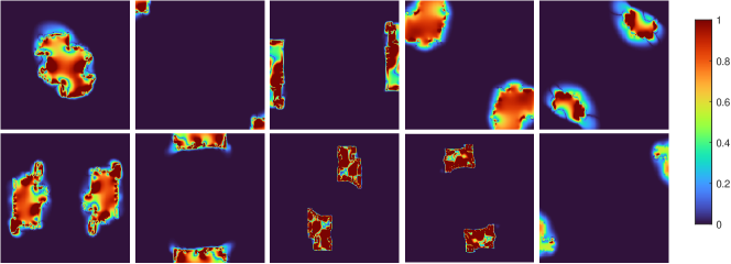
((a))

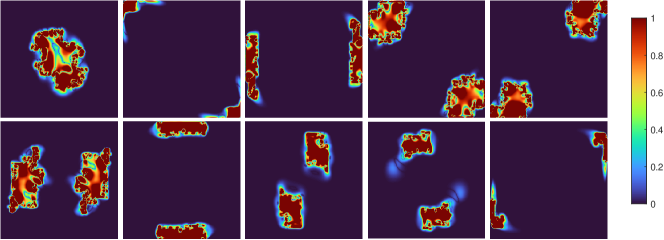
((b))

((c))

Figure 4: Normalized wavelet systems. Normalized disk band-pass empirical wavelet filters $\widehat{\chi}_{n}^{\mathrm{D},\tau}$ with $\tau=0.2$ for the Watershed partition and the different mapping estimators.

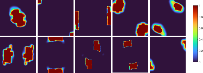
((a))

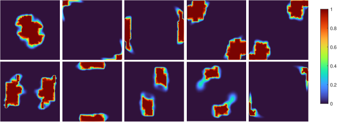
((b))

((c))

Figure 5: Unnormalized wavelet systems. Unnormalized disk band-pass empirical wavelet filters $\widehat{\chi}_{n}^{\mathrm{D},\tau}$ with $\tau=0.2$ for the Watershed partition and the different mapping estimators.

In conclusion, the additive demons provides accurate continuous mapping estimates to compute robust unnormalized empirical wavelet filters in a reasonable computation time. As for the diffeomorphic demons, it provides inaccurate diffeomorphic mapping estimates, leading to unsuitable normalized filters.

4.4 Reconstruction assessment

To assess the numerical behavior of the empirical wavelet transform, which is theoretically lossless for the disk and square band-pass filter according to Theorem 2, we examinate the quality of reconstruction. Table 3 reports the PSNR of the empirical wavelet reconstruction of the toy image for the disk and square band-pass filters with different transition widths $\tau$, the Watershed and Voronoi partitions and the different demons algorithms. The additive demons provides better or at least similar reconstruction than the other demons. Moreover, the normalization in the empirical wavelet filters has no impact on the reconstruction performance for the different demons.

Despite the accuracy of the mapping estimation obtained in Table 1, the related wavelet reconstruction can be corrupted when the estimated filter bank is not entirely covering the Fourier domain. Notably, the transition width $\tau=0.2$ permits to ensure a larger covering of the Fourier domain than the transition width $\tau=0.1$ by the filters in case of an inaccurate estimate of a mapping. In contrast, the transition width $\tau=0.3$ can lead to artefacts in a symmetric wavelet $\chi_{n}$ due to overlaps of paired wavelet filters $\widehat{\psi}_{n}$ and $\widehat{\psi}_{-n}$, as observed for the disk band-pass transform using the Watershed partition and a diffeomorphic demons.

Table 3: PSNR of the reconstructed images for the different demons algorithms, sets $\Lambda$, partitioning methods and transition widths $\tau$ for the normalized and unnormalized empirical wavelet transforms.

Demons	$\boldsymbol{\tau}$	Normalized				Unnormalized
		Watershed		Voronoi		Watershed		Voronoi
		Disk	Square	Disk	Square	Disk	Square	Disk	Square
Thirion’s	$0.1$	$76.21$	$\mathbf{79.67}$	$82.61$	$90.79$	$76.21$	$\mathbf{79.67}$	$82.63$	$90.79$
Additive		$\mathbf{96.08}$	$79.23$	$\mathbf{120.47}$	$\mathbf{305.64}$	$\mathbf{96.08}$	$79.23$	$\mathbf{120.47}$	$\mathbf{306.03}$
Diffeomorphic		$89.20$	$62.05$	$97.88$	$286.93$	$89.20$	$62.05$	$97.12$	$269.60$
Thirion’s	$0.2$	$78.22$	$87.21$	$85.34$	$297.90$	$78.22$	$87.22$	$85.34$	$302.70$
Additive		$\mathbf{112.78}$	$\mathbf{305.65}$	$\mathbf{305.47}$	$\mathbf{305.69}$	$\mathbf{112.78}$	$\mathbf{305.88}$	$\mathbf{306.37}$	$\mathbf{306.26}$
Diffeomorphic		$89.20$	$124.85$	$103.42$	$303.76$	$89.20$	$120.77$	$101.77$	$305.40$
Thirion’s	$0.3$	$85.02$	$180.79$	$89.32$	$305.10$	$84.82$	$183.43$	$89.32$	$305.39$
Additive		$\mathbf{124.41}$	$\mathbf{305.16}$	$\mathbf{305.78}$	$\mathbf{305.61}$	$\mathbf{124.41}$	$\mathbf{305.67}$	$\mathbf{306.00}$	$\mathbf{306.16}$
Diffeomorphic		$77.27$	$117.87$	$103.45$	$303.19$	$64.14$	$128.81$	$103.38$	$305.38$

4.5 Application to texture segmentation

Analyzing the structure and chemical properties of self-assembled monolayers of organic molecules is the core of many applications in nanoscience and nanotechnology [17, 10]. These properties result in variations in the textures that are crucial to identify. Recently, Empirical Curvelet Wavelet Transform (EWT-Curvelet), obtained by partitioning the Fourier domain in scales and angles [9], has shown to provide relevant texture features for scanning tunneling microscope images of self-assembled monolayers [11, 2]. In this section, we explore the relevance of the proposed Empirical Wavelet Transform for this task.

used the proposed approach to characterize patterns of cyanide molecules [11, 12]

We perform the texture segmentation according to the procedure of [14], which consists of the following steps. First, we extract the textural part of the images by performing a cartoon–texture decomposition [1, 8]. Next, we perform an empirical wavelet transform and compute the local energy of the obtained coeficients which is the average of the coefficients over a window of size $19\times 19$ at each pixel. Finally, segmentation is obtained by performing a pixel-wise k-means clustering with cityblock distance for preselected numbers of cluster $k$ on the local energy.

Figure 6 shows partitions of the Fourier spectrum of a scanning tunneling microscope image obtained by the Curvelet, Watershed and Voronoi methods with a scale-space step-size $s_{0}=0.8$ on the logarithm of the Fourier spectrum. The Curvelet method results in a large number of sets $\Omega_{n}$, namely $393$, while the Watershed and Voronoi methods extract as many sets $\Omega_{n}$ as detected harmonic modes, $17$ in this case.

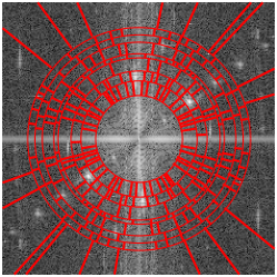
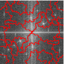
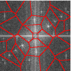
Figure 6: Examples of Fourier partitions. Fourier spectrum of a scanning tunnelling microscope image overlapped with partitions obtained by the Curvelet (left), Watershed (middle) and Voronoi (right) methods.

Figure 7 shows scanning tunneling microscope images, their corresponding texture parts, and their segmentation for the EWT-Curvelet and the proposed disk and square band-pass empirical wavelet transforms with $\tau=0.2$ for both Voronoi and Watershed partitioning. The proposed empirical wavelet transforms provide accurate and comparable texture masks for the different images. In all cases, the segmentation performance with the proposed approach is better than with the EWT-Curvelet, as can be clearly seen in the last two rows of Figure 7.

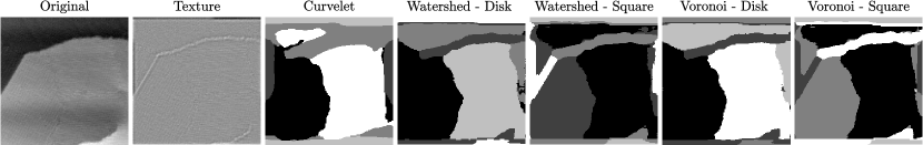
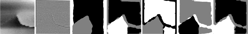
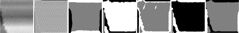
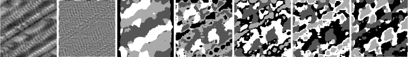
Figure 7: Texture segmentation. Original scanning tunneling microscope images, their textural parts and the segmentation obtained for the different empirical wavelet transforms with numbers of clusters $k$ set to $5$, $3$, $3$ and $4$ from top to bottom, respectively. Raw scanning tunneling microscope images of cyanide on Au$\{111\}$ have been reproduced from [11, 12] with permission. Images copyright American Chemical Society.

5 Discussion

The proposed numerical implementation based on the additive demons algorithm provides accurate continuous mappings suitable for the empirical wavelet transform. The results show that this approach has satisfactory performances for reconstruction and texture extraction. In contrast, diffeomorphic mapping estimates are harder and longer to obtain. This suggests to avoid in practice the use of normalization proposed in previous work [18].

The proposed algorithm applies for any homogeneous or separable wavelet kernel and any Fourier partition. However, the selection of the wavelet kernel’s support and the partitioning method is crucial to optimize the mapping estimation performance. The study conducted in the present work shows that a Voronoi partition and a wavelet kernel defined on a disk result in a better performance overall.

The proposed numerical procedure is ready for application on real-world data. In particular, it has shown to provide relevant texture features for scanning tunneling microscope images for the different studied wavelet kernels. In addition, the number of features resulting from the Voronoi or Watershed partitioning methods is reasonnable compared to the one obtained by the Curvelet transform used in [2].

Future work will include a thorough study of the stop criterion of the additive demons algorithm and the use of different wavelet kernels in applications.

6 Conclusions

This work proposed an efficient algorithm for the empirical wavelet transform from any wavelet kernel based on demons registration. Among the different meticulously compared demons algorithms, the additive one has shown to provide accurate numerical empirical wavelet systems with good properties of reconstruction, as validated for suitable wavelet kernels. The relevance of this approach for texture feature extraction has also been highlighted. A Matlab toolbox will be made publicly available at the time of publication.

7 Acknowledgement

This work was funded by the Air Force Office of Scientific Research, grant FA9550-21-1-0275.

References

- [1] Jean-François Aujol and Tony F Chan. Combining geometrical and textured information to perform image classification. Journal of Visual Communication and Image Representation, 17(5):1004–1023, 2006.
- [2] Kevin Bui, Jacob Fauman, David Kes, Leticia Torres Mandiola, Adina Ciomaga, Ricardo Salazar, Andrea L Bertozzi, Jérôme Gilles, Dominic P Goronzy, Andrew I Guttentag, and P.S. Weiss. Segmentation of scanning tunneling microscopy images using variational methods and empirical wavelets. Pattern Analysis and Applications, 23:625–651, 2020.
- [3] Pascal Cachier, Eric Bardinet, Didier Dormont, Xavier Pennec, and Nicholas Ayache. Iconic feature based nonrigid registration: the pasha algorithm. Computer vision and image understanding, 89(2-3):272–298, 2003.
- [4] Bhaswati Singha Deo, Mayukha Pal, Prasanta K Panigrahi, and Asima Pradhan. An ensemble deep learning model with empirical wavelet transform feature for oral cancer histopathological image classification. International Journal of Data Science and Analytics, pages 1–18, February 2024.
- [5] Jérôme Gilles. Empirical wavelet transform. IEEE Transactions on Signal Processing, 61(16):3999–4010, August 2013.
- [6] Jérôme Gilles. Empirical voronoi wavelets. Constructive Mathematical Analysis, 5(4):183–189, 2022.
- [7] Jérôme Gilles and Kathryn Heal. A parameterless scale-space approach to find meaningful modes in histograms - application to image and spectrum segmentation. International Journal of Wavelets, Multiresolution and Information Processing, 12(6):1450044, 2014.
- [8] Jérôme Gilles and Stanley Osher. Bregman implementation of meyer’s g-norm for cartoon+ textures decomposition. UCLA Cam Report, pages 11–73, 2011.
- [9] Jérôme Gilles, Giang Tran, and Stanley Osher. 2D Empirical transforms. Wavelets, Ridgelets and Curvelets Revisited. SIAM Journal on Imaging Sciences, 7(1):157–186, January 2014.
- [10] J Justin Gooding, Freya Mearns, Wenrong Yang, and Jingquan Liu. Self-assembled monolayers into the 21st century: recent advances and applications. Electroanalysis: An International Journal Devoted to Fundamental and Practical Aspects of Electroanalysis, 15(2):81–96, 2003.
- [11] Andrew I Guttentag, Kristopher K Barr, Tze-Bin Song, Kevin V Bui, Jacob N Fauman, Leticia F Torres, David D Kes, Adina Ciomaga, Jérôme Gilles, Nichole F Sullivan, et al. Hexagons to ribbons: Flipping cyanide on au 111. Journal of the American Chemical Society, 138(48):15580–15586, 2016.
- [12] Andrew I Guttentag, Tobias Wächter, Kristopher K Barr, John M Abendroth, Tze-Bin Song, Nichole F Sullivan, Yang Yang, David L Allara, Michael Zharnikov, and Paul S Weiss. Surface structure and electron transfer dynamics of the self-assembly of cyanide on au 111. The Journal of Physical Chemistry C, 120(47):26736–26746, 2016.
- [13] Norden E Huang, Zheng Shen, Steven R Long, Manli C Wu, Hsing H Shih, Quanan Zheng, Nai-Chyuan Yen, Chi Chao Tung, and Henry H Liu. The empirical mode decomposition and the hilbert spectrum for nonlinear and non-stationary time series analysis. Proceedings of the Royal Society of London. Series A: mathematical, physical and engineering sciences, 454(1971):903–995, 1998.
- [14] Yuan Huang, Valentin De Bortoli, Fugen Zhou, and Jérôme Gilles. Review of wavelet-based unsupervised texture segmentation, advantage of adaptive wavelets. IET Image Processing, 12(9):1626–1638, 2018.
- [15] Yuan Huang, Fugen Zhou, and Jérôme Gilles. Empirical curvelet based fully convolutional network for supervised texture image segmentation. Neurocomputing, 349:31–43, 2019.
- [16] Basile Hurat, Zariluz Alvarado, and Jérôme Gilles. The empirical watershed wavelet. Journal of Imaging, 6(12):140, 2020.
- [17] J Christopher Love, Lara A Estroff, Jennah K Kriebel, Ralph G Nuzzo, and George M Whitesides. Self-assembled monolayers of thiolates on metals as a form of nanotechnology. Chemical reviews, 105(4):1103–1170, 2005.
- [18] Charles-Gérard Lucas and Jérôme Gilles. Multidimensional empirical wavelet transform. arXiv preprint arXiv:2405.06188, 2024.
- [19] Shishir Maheshwari, Ram Bilas Pachori, and U Rajendra Acharya. Automated diagnosis of glaucoma using empirical wavelet transform and correntropy features extracted from fundus images. IEEE journal of biomedical and health informatics, 21(3):803–813, 2016.
- [20] T V Nidhin Prabhakar and P Geetha. Two-dimensional empirical wavelet transform based supervised hyperspectral image classification. ISPRS Journal of Photogrammetry and Remote Sensing, 133:37–45, November 2017.
- [21] Deepak Parashar and Dheeraj Kumar Agrawal. Automatic classification of glaucoma stages using two-dimensional tensor empirical wavelet transform. IEEE Signal Processing Letters, 28:66–70, 2020.
- [22] Srinivasu Polinati and Ravindra Dhuli. Multimodal medical image fusion using empirical wavelet decomposition and local energy maxima. Optik, 205:163947, March 2020.
- [23] K Joseph Abraham Sundar, Motepalli Jahnavi, and Konudula Lakshmisaritha. Multi-sensor image fusion based on empirical wavelet transform. In 2017 International Conference on Electrical, Electronics, Communication, Computer, and Optimization Techniques (ICEECCOT), pages 93–97. IEEE, 2017.
- [24] J-P Thirion. Image matching as a diffusion process: an analogy with Maxwell’s demons. Medical image analysis, 2(3):243–260, 1998.
- [25] Tom Vercauteren, Xavier Pennec, Aymeric Perchant, and Nicholas Ayache. Diffeomorphic demons: Efficient non-parametric image registration. NeuroImage, 45(1):S61–S72, 2009.