Analytic weak-signal approximation of the Bayes factor for continuous gravitational waves

Abstract

We generalize the targeted $\mathcal{B}$-statistic for continuous gravitational waves by modeling the $h_{0}$-prior as a half-Gaussian distribution with scale parameter $H$. This approach retains analytic tractability for two of the four amplitude marginalization integrals and recovers the standard $\mathcal{B}$-statistic in the strong-signal limit ($H\rightarrow\infty$). By Taylor-expanding the weak-signal regime ($H\rightarrow 0$), the new prior enables fully analytic amplitude marginalization, resulting in a simple, explicit statistic that is as computationally efficient as the maximum-likelihood $\mathcal{F}$-statistic, but significantly more robust. Numerical tests show that for day-long coherent searches, the weak-signal Bayes factor achieves sensitivities comparable to the $\mathcal{F}$-statistic, though marginally lower than the standard $\mathcal{B}$-statistic (and the Bero-Whelan approximation). In semi-coherent searches over short (compared to a day) segments, this approximation matches or outperforms the weighted dominant-response $\widehat{\mathcal{F}}_{\mathrm{ABw}}$-statistic and returns to the sensitivity of the (weighted) $\widehat{\mathcal{F}}_{\mathrm{w}}$-statistic for longer segments. Overall the new Bayes-factor approximation demonstrates state-of-the-art or improved sensitivity across a wide range of segment lengths we tested (from $900\text{\,}\mathrm{s}$ to $10\text{\,}\mathrm{d}\mathrm{a}\mathrm{y}\mathrm{s}$).

[2024-09-19 21:38:02 +0200; commitID: 5872a64-UNCLEAN]

1 Introduction

Continuous gravitational waves (CWs), expected to be emitted by spinning non-axisymmetric neutron stars in our galaxy, are one of the most anticipated but still undetected types of gravitational waves. Finding CWs will mark the culmination of decades of research aimed at refining search methods and applying them to data from ground-based detectors, such as LIGO Hanford (H1), Livingston (L1) [1], and Virgo (V1) [2]. For recent reviews, see, for example, [3, 4].

CW signals manifest in the detector data as amplitude-modulated quasi-sinusoidal waveforms with slowly varying (generally decreasing) frequency. These are long-lasting but extremely weak signals compared to the detector noise, and will therefore require combining months to years of data to become detectable. The signals are characterized by four amplitude parameters: the overall amplitude $h_{0}$, two polarization angles $\iota$ and $\psi$, and the initial phase $\phi_{0}$. An additional set of phase-evolution parameters, such as the frequency (and its time derivatives), sky position and binary-orbital parameters, is required to fully determine the signal, depending on the search space considered.

A key research focus for detecting CWs is the development of statistics that maximize the detection probability at a fixed false-alarm level, while being as computationally efficient as possible. A significant milestone in this area was the seminal work by Jaranowski, Królak, and Schutz [5] (henceforth “JKS”), demonstrating that the likelihood ratio can be analytically maximized over the four unknown amplitude parameters after a coordinate transformation. This results in the $\mathcal{F}$-statistic, which only requires explicit searches over phase-evolution parameters, thereby substantially reducing the computing cost. Another closely-related coherent statistic was constructed by different arguments within the “5-vector” formalism [6], equally dispensing with the amplitude parameters and resulting in very similar detection power.

Searle pointed out in [7] that for composite signal hypotheses (i.e., those with unknown parameters), the Neyman-Pearson lemma shows that the optimal statistic is the marginalized (rather than maximized) likelihood ratio, also known as the Bayes factor. This was illustrated in the CW context in [8], showing that marginalizing with more physical priors over the amplitude parameters resulted in a (slightly) more powerful statistic (referred to as the $\mathcal{B}$-statistic) than the $\mathcal{F}$-statistic. However, this statistic entails a substantially higher computing cost, given that only two of the four marginalization integrals have been solved analytically [9], while the remaining two need to be performed numerically. There have been a number of attempts [10, 11, 12, 13] to find usable solutions and approximations to these integrals, with the most successful fully-analytic approximation to date provided by Bero & Whelan [14].

On the other hand, recent work [15] on semi-coherent all-sky searches for neutron stars in unknown binary systems has revealed some unexpected weaknesses of the $\mathcal{F}$-statistic: the extreme computational cost of these searches requires using very short segments, of order $\mathcal{O}\left($100\text{\,}\mathrm{s}$\right)$. Surprisingly, the $\mathcal{F}$-statistics turns out to be quite sub-optimal for such short segments, and an empirically-constructed dominant-response statistic $\mathcal{F}_{\mathrm{AB}}$, effectively dropping two of the four amplitude degrees of freedom, was shown in [16] to beat the $\mathcal{F}$-statistic sensitivity by up to $\sim$19\text{\,}\mathrm{\char 37\relax}$$ in the short-segment limit. Furthermore, when signal power varies over segments, which can happen both due to varying (i) antenna-pattern response, and (ii) noise floors and duty factors, then an explicit segment-weighting scheme was shown in [17] to improve sensitivity over the conventional directly-summed semi-coherent $\widehat{\mathcal{F}}$- (or $\widehat{\mathcal{F}}_{\mathrm{AB}}$) statistics.

These empirical findings raise the question of how to understand and leverage them within the Bayesian framework. Given that three of the four amplitude parameters (namely $\iota,\psi,\phi_{0}$) have well-defined ignorance priors [8], the only remaining freedom left is the choice of $h_{0}$-prior. Previous works on the CW Bayes factor have all used a uniform $h_{0}$-prior, for simplicity and because it enables analytical marginalization. However, this is intrinsically a “strong-signal” prior, in the sense that it puts more probability weight on larger orders of magnitude compared to smaller ones.

Here we explore a new $h_{0}$-prior in the form of a half-Gaussian with scale parameter $H$, which is more “physical” in the sense of giving more weight to smaller $h_{0}$ amplitudes compared to larger ones. This contains the uniform prior in the asymptotic strong-signal limit ($H\rightarrow\infty$), while preserving the ability for analytic $h_{0}$ integration. In the “weak-signal” limit ($H\rightarrow 0$), we can Taylor-expand in small $H$ and obtain a fully analytic solution for all four Bayes- factor integrals. Used as a semi-coherent statistic, this performs as well and better than the weighted $\widehat{\mathcal{F}}_{\mathrm{ABw}}$ statistic for short segments and the weighted $\mathcal{F}$-statistic $\widehat{\mathcal{F}}_{\mathrm{w}}$ for long segments.

The plan of this paper is as follows: introduction to the $\mathcal{F}$-statistic formalism in Sec. 2, followed by a recap of the corresponding Bayesian formalism in Sec. 3 with $\mathcal{B}$-statistic and Bero&Whelan approximation. Derivation of the new generalized $\mathcal{B}$-statistic and analytic weak-signal approximation in Sec. 4. Derivation of the weak-signal statistic as a generalized $\chi^{2}$-distribution in Sec. 5, followed by numerical tests and results presented in Sec. 6, with conclusions in Sec. 7.

2 The $\mathcal{F}$-statistic formalism

2.1 Signal model

The signal depends on amplitude parameters $\mathcal{A}\equiv\{h_{0},\eta,\psi,\phi_{0}\}$, where $h_{0}$ is the overall amplitude, $\eta\equiv\cos\iota$ quantifies the degree of circular polarization in terms of the inclination angle $\iota$ of the neutron-star spin axis to the line of sight, $\psi$ describes the polarization in terms of its rotation angle on the sky, and $\phi_{0}$ is the signal phase at a reference time (see [9] for a more detailed discussion of the geometry). We refer to this parametrization as the physical amplitude coordinates.

The seminal paper [5] introduced a new set of amplitude coordinates $\{\mathcal{A}^{\mu}\}$, referred to as JKS coordinates, which are defined as

$$\eqalign{\mathcal{A}^{1}&\equiv\hskip 6.99997ptA_{+}\cos\phi_{0}\cos 2\psi-A_{\times}\sin\phi_{0}\sin 2\psi\,,\\ \mathcal{A}^{2}&\equiv\hskip 6.99997ptA_{+}\cos\phi_{0}\sin 2\psi+A_{\times}\sin\phi_{0}\cos 2\psi\,,\\ \mathcal{A}^{3}&\equiv-A_{+}\sin\phi_{0}\cos 2\psi-A_{\times}\cos\phi_{0}\sin 2\psi\,,\\ \mathcal{A}^{4}&\equiv-A_{+}\sin\phi_{0}\sin 2\psi+A_{\times}\cos\phi_{0}\cos 2\psi\,,}$$ (1)

in terms of the polarization amplitudes $A_{+}\equiv h_{0}\,(1+\eta^{2})/2$ and $A_{\times}\equiv h_{0}\,\eta$. Using these coordinates, the signal $h(t)$ in the detector frame takes the linear form

$$h(t;\mathcal{A},\lambda)=\mathcal{A}^{\mu}\,h_{\mu}(t;\lambda),$$ (2)

with automatic summation over repeated amplitude indices $\mu=1,\ldots,4$, and with four matched-filter basis functions $h_{\mu}(t;\lambda)$ defined as

$$\eqalign{h_{1}(t)&\equiv a(t)\,\cos\phi(t),\quad h_{2}(t)\equiv b(t)\,\cos\phi(t),\\ h_{3}(t)&\equiv a(t)\,\sin\phi(t),\quad h_{4}(t)\equiv b(t)\,\sin\phi(t),}$$ (3)

in terms of the signal phase $\phi(t;\lambda)$ at the detector with sky-direction dependent antenna-pattern functions $a(t;\vec{n}),\,b(t;\vec{n})$ (cf. [5, 18] for explicit expressions).

The phase-evolution parameters $\lambda$ include the remaining signal parameters, namely the sky-position $\vec{n}$, frequency $f$ and higher-order derivatives $\dot{f},\ddot{f},\ldots$ at some given reference time, describing the slowly-changing intrinsic signal frequency. For CW sources in binary systems $\lambda$ also includes the binary orbital parameters. The sky position $\vec{n}$ is most commonly specified in terms of the equatorial longitude $\alpha$ and latitude $\delta$, measured in radians.

Here we only consider the standard “mountain” emission model, where the gravitational-wave frequency $f=2\nu$ is twice the rotation frequency $\nu$ of the neutron star, with discussion of free-precession (with additional emission at $f\approx\nu$) and r-modes (with $f\approx{4\nu}/{3}$) postponed to future work.

2.2 Likelihood ratio

We want to construct the optimal detection statistic for distinguishing between the Gaussian-noise hypothesis $\mathcal{H}_{\mathrm{G}}:x(t)=n(t)$, when the data $x$ contains only Gaussian noise $n$, and the signal hypothesis $\mathcal{H}_{\mathrm{S}}:x(t)=n(t)+h(t;\mathcal{A},\lambda)$, when there is an additional signal $h(t;\mathcal{A},\lambda)$ of the form (2). Optimality of a statistic $S(x)$ is defined in terms of the Neyman-Pearson criterion of maximizing the detection probability $p_{\mathrm{det}}=P\left(S>S_{\mathrm{thr}}|\mathcal{H}_{\mathrm{S}}\right)$ at a fixed false-alarm probability $p_{\mathrm{fa}}\equiv P\left(S>S_{\mathrm{thr}}|\mathcal{H}_{\mathrm{G}}\right)$, parametrized in terms of a detection threshold $S_{\mathrm{thr}}$.

For two simple hypothesis, i.e., with no unknown parameters, the classic Neyman-Pearson lemma [19] proves that the optimal statistic is the likelihood ratio, namely

$$\mathcal{L}(x;\mathcal{A},\lambda)\equiv\frac{P\left(x|\mathcal{H}_{\mathrm{S}},\mathcal{A},\lambda\right)}{P\left(x|\mathcal{H}_{\mathrm{G}}\right)}=\exp\left[\left(x|h\right)-\frac{1}{2}\left(h|h\right)\right],$$ (4)

where the last expression holds for the specific hypotheses $\mathcal{H}_{\mathrm{G}},\mathcal{H}_{\mathrm{S}}$ being considered here, and we introduced the “matched-filter” scalar product $\left(x|y\right)$, see [20].

The scalar product for narrow-band signals (such as CWs) in a single detector with stationary noise floor and no gaps in the data, would simply be $\left(x|y\right)\equiv 2\mathcal{S}^{-1}\int_{0}^{T_{\mathrm{data}}}x(t)\,y(t)\,dt$, in terms of the (single-sided) noise power spectral density $\mathcal{S}(f)$ around the signal frequency $f$ and data duration $T_{\mathrm{data}}$. One can generalize this to several detectors, allowing for gaps in the data and non-stationary noise-floors (see B for the full expression), and still write it in the form

$$\left(x|y\right)\equiv 2\gamma\,\langle{x\,y}\rangle\,,$$ (5)

in terms of a (weighted) multi-detector average $\langle{\ldots}\rangle$ and a dimensionless data factor $\gamma$ [18, 16], which we define as

$$\gamma\equiv\mathcal{S}^{-1}\,T_{\mathrm{data}},$$ (6)

which can be understood as the product of the data “quality” (i.e., $\mathcal{S}^{-1}$) and “quantity”, $T_{\mathrm{data}}$. Note that this involves the non-stationary generalization of the overall noise floor $\mathcal{S}$ given in (95).

Substituting the JKS signal form (2), we can express the log-likelihood ratio as

$$\ln\mathcal{L}(x;\mathcal{A},\lambda)=\mathcal{A}^{\mu}x_{\mu}-\frac{1}{2}\mathcal{A}^{\mu}\mathcal{M}_{\mu\nu}\mathcal{A}^{\nu}\,,$$ (7)

where we defined

$$x_{\mu}\equiv\left(x|h_{\mu}\right),\quad\text{and}\quad\mathcal{M}_{\mu\nu}\equiv\left(h_{\mu}|h_{\nu}\right).$$ (8)

The four numbers $x_{\mu}$ are the scalar products of the data $x$ matched against the basis functions $h_{\mu}$ of (3), while the detector-response matrix $\mathcal{M}_{\mu\nu}$ can be expressed more explicitly as

$$\mathcal{M}=\gamma M=\gamma\left(\begin{array}[]{cc}m&0\\ 0&m\\ \end{array}\right),\quad\text{with}\quad m\equiv\left(\begin{array}[]{cc}A&C\\ C&B\\ \end{array}\right),$$ (9)

where $A=\langle{a^{2}}\rangle$, $B=\langle{b^{2}}\rangle$, and $C=\langle{a\,b}\rangle$ are the (sky-position dependent) averaged antenna-pattern coefficients. This expression shows two contributions to the detector response, namely the data factor $\gamma$ and a geometric antenna-pattern matrix $M$, encoding the detector sensitivity to a particular sky direction (integrated over the available observation time). We can express the determinant as

$$\det\mathcal{M}=\gamma^{4}\,D^{2}\,\quad\text{with}\quad D\equiv\det m=AB-C^{2}\,.$$ (10)

In practice the amplitude parameters $\mathcal{A}$ are (generally) unknown, and depending on the type of search, also some or all of the phase-evolution parameters. The signal hypothesis $\mathcal{H}_{\mathrm{S}}$ is therefore always a composite hypothesis involving unknown parameters. Therefore the likelihood ratio (4) is a function of these unknown parameters and cannot be directly used as a detection statistic.

2.3 The $\mathcal{F}$-statistic

A classic method for dealing with composite hypotheses is the maximum-likelihood approach, which consists of using the maximized likelihood ratio as a detection statistic. Applying this approach to (7), one can analytically maximize $\mathcal{L}$ over the JKS amplitude parameters $\mathcal{A}^{\mu}$ and obtain

$$\mathcal{F}(x;\lambda)\equiv\max_{\{\mathcal{A}^{\mu}\}}\ln\mathcal{L}(x;\mathcal{A},\lambda)=\frac{1}{2}x_{\mu}\left(\mathcal{M}^{-1}\right)^{\mu\nu}x_{\nu},$$ (11)

defining the $\mathcal{F}$-statistic [5], with the corresponding maximum-likelihood estimators $\hat{\mathcal{A}}^{\mu}$ for the amplitude parameters given by

$$\hat{\mathcal{A}}^{\mu}\equiv\left(\mathcal{M}^{-1}\right)^{\mu\nu}x_{\mu}\,.$$ (12)

This statistic can be shown [5] to follow a $\chi^{2}$-distribution with four degrees of freedom, and noncentrality parameter

$$\rho^{2}\equiv\left(h|h\right)=\mathcal{A}^{\mu}\mathcal{M}_{\mu\nu}\mathcal{A}^{\nu},$$ (13)

which we refer to as the signal power, also commonly known as the squared signal-to-noise ratio (SNR) in this context.

3 Bayesian detection framework

3.1 Bayes factor

Unlike the ad-hoc maximum-likelihood approach discussed earlier, the Bayesian framework offers a natural and unique method for handling unknown parameters, grounded in the three fundamental laws of probability [21].

The likelihood for a composite signal hypothesis $\mathcal{H}_{\mathrm{S}}$ can be directly obtained as

$$P\left(x|\mathcal{H}_{\mathrm{S}}\right)=\int P\left(x|\mathcal{H}_{\mathrm{S}},\mathcal{A},\lambda\right)\,P\left(\mathcal{A},\lambda|\mathcal{H}_{\mathrm{S}}\right)\,d\mathcal{A}\,d\lambda,$$ (14)

also referred to as the marginalized likelihood, which requires an explicit specification of the prior probabilities for the unknown signal parameters $\{\mathcal{A},\lambda\}$. Assuming for simplicity a Gaussian-noise hypothesis with known noise floor $\mathcal{S}$, this further leads to the marginalized likelihood ratio

$$B_{\mathrm{{\mathrm{S}}/{\mathrm{G}}}}(x)\equiv\frac{P\left(x|\mathcal{H}_{\mathrm{S}}\right)}{P\left(x|\mathcal{H}_{\mathrm{G}}\right)}=\int\mathcal{L}(x;\mathcal{A},\lambda)\,P\left(\mathcal{A},\lambda|\mathcal{H}_{\mathrm{S}}\right)\,d\mathcal{A}\,d\lambda,$$ (15)

commonly known as the Bayes factor between the signal and the Gaussian-noise hypothesis.

Here we focus exclusively on the marginalization over amplitude parameters $\mathcal{A}$, and therefore consider only a single phase-evolution point $\lambda$ in the following. This could be interpreted as a “targeted” search scenario, but could equally represent simply a single template step in a wide-parameter space search.

3.2 Rediscovering the $\mathcal{F}$-statistic

Building on the pioneering work [22, 23] in burst searches, [8] demonstrated that the $\mathcal{F}$-statistic can also be derived as a Bayes factor, assuming a (somewhat arbitrary) prior that is uniform in $\mathcal{A}^{\mu}$-space. Specifically, $P\left(\{\mathcal{A}^{\mu}\}|\mathcal{H}_{\mathrm{S}}\right)=k$, leading to a Gaussian integral that yields

$$B_{\mathrm{{\mathrm{S}}/{\mathrm{G}}}}(x;\lambda)=k\frac{4\pi^{2}}{\sqrt{\det\mathcal{M}}}e^{\mathcal{F}(x;\lambda)}\,.$$ (16)

The Jacobian for the coordinate transformation (1) between $\mathcal{A}^{\mu}$ and physical amplitude parameters can be obtained [8, 9] as

$$P\left(h_{0},\eta,\psi,\phi_{0}|\mathcal{H}_{\mathrm{S}}\right)=\frac{1}{4}h_{0}^{3}\left(1-\eta^{2}\right)^{3}P\left(\{\mathcal{A}^{\mu}\}|\mathcal{H}_{\mathrm{S}}\right)\,,$$ (17)

therefore a constant-$\mathcal{A}^{\mu}$ prior favors signals with large $h_{0}$ and linear polarization ($\eta\sim 0$) over circular polarization $\eta\sim\pm 1$, both of which are unphysical.

In order to be normalizable, this prior needs to be artificially truncated at some large-$\mathcal{A}^{\mu}$ surface. One can also use this to (arbitrarily) remove the prefactor by choosing an $\mathcal{M}$-dependent truncation surface, as discussed in [24], resulting in a $\mathcal{F}$-statistic Bayes factor of the form $B_{\mathrm{{\mathrm{S}}/{\mathrm{G}}}}(x;\lambda)=k^{\prime}\,e^{\mathcal{F}(x;\lambda)}$ instead, where the prefactor $k^{\prime}$ is now independent of the detector-response matrix $\mathcal{M}$. Empirically this form was found to result in better performance on transient-CW signals [24], and was also used as the basis for constructing extended “line-robust” Bayes factors in [25, 26].

3.3 Neyman-Pearson-Searle optimality

As Searle noted in [7], the Neyman-Pearson proof for the optimal detection statistic only requires the likelihoods for the two competing hypotheses. Since the Bayesian framework uniquely provides a marginalized likelihood (14) for the composite signal hypothesis, it follows that the marginalized likelihood ratio (7) (i.e., the Bayes factor) is the Neyman-Pearson optimal statistic, assuming the unknown signal parameters are drawn from the priors.

Thus, the somewhat unphysical prior of Sec. 3.2 implies that the $\mathcal{F}$-statistic is not optimal, and using more appropriate priors can lead to a more powerful detection statistic. This was demonstrated in [8], where an isotropic prior on the neutron star’s spin orientation (reflecting our ignorance of the spin axis) was used instead, namely

$$P\left(h_{0},\eta,\psi,\phi_{0}|\mathcal{H}_{\mathrm{S}}\right)=\frac{1}{2\pi^{2}}\,P\left(h_{0}|\mathcal{H}_{\mathrm{S}}\right)\,,$$ (18)

which is uniform in $\eta\in[-1,1]$, $\psi\in[-\pi/4,\pi/4]$ and $\phi_{0}\in[0,2\pi]$. We can therefore write the general form of the optimal Bayes factor as

$$B_{\mathrm{{\mathrm{S}}/{\mathrm{G}}}}(x;\lambda)\equiv\frac{1}{2\pi^{2}}\int\mathcal{L}(x;\lambda,\mathcal{A})\,P\left(h_{0}\right)\,dh_{0}\,d\eta\,d\psi\,d\phi_{0}\,.$$ (19)

The correct choice for an $h_{0}$-prior is less obvious and would ultimately have to be constructed from astrophysical arguments about the expected distance, rotation rate and deformation of neutron stars. Generally speaking, however, we expect a “physical” $h_{0}$-prior to favor weaker signals over stronger ones, contrary to the implicit $\mathcal{F}$-statistic prior $\propto h_{0}^{3}$ of (17).

3.4 Likelihood ratio in physical coordinates

In order to make progress on the Bayes-factor integral (19), it is useful to express the likelihood ratio $\mathcal{L}$ of (7) in terms of the physical amplitude parameters $\{h_{0},\eta,\psi,\phi_{0}\}$. This can be obtained [9] in the following form,

$$\ln\mathcal{L}(x;\mathcal{A})=h_{*}\,q(x;\eta,\psi)\,\cos\left(\phi_{0}-\varphi_{0}\right)-\frac{1}{2}h_{*}^{2}\,g^{2}(\eta,\psi),$$ (20)

where we defined the relative signal amplitude $h_{*}$ as

$$h_{*}\equiv h_{0}\sqrt{\gamma}=h_{0}\sqrt{\frac{T_{\mathrm{data}}}{\mathcal{S}}}\,,$$ (21)

and the geometric response function

$$g^{2}(\eta,\psi)\equiv\alpha_{1}\,A+\alpha_{2}\,B+2\alpha_{3}\,C\,,$$ (22)

in terms of the amplitude coefficients $\alpha_{i}(\eta,\psi)$:

$$\eqalign{\alpha_{1}(\eta,\psi)&\equiv\frac{(\mathcal{A}^{1})^{2}+(\mathcal{A}^{3})^{2}}{h_{0}^{2}}=\frac{1}{4}(1+\eta^{2})^{2}\,\cos^{2}2\psi+\eta^{2}\,\sin^{2}2\psi,\\ \alpha_{2}(\eta,\psi)&\equiv\frac{(\mathcal{A}^{2})^{2}+(\mathcal{A}^{4})^{2}}{h_{0}^{2}}=\frac{1}{4}(1+\eta^{2})^{2}\,\sin^{2}2\psi+\eta^{2}\,\cos^{2}2\psi,\\ \alpha_{3}(\eta,\psi)&\equiv\frac{\mathcal{A}^{1}\mathcal{A}^{2}+\mathcal{A}^{3}\mathcal{A}^{4}}{h_{0}^{2}}=\frac{1}{4}(1-\eta^{2})^{2}\,\sin 2\psi\cos 2\psi.}$$ (23)

This allows us to write the signal power $\rho^{2}$ of (13) as

$$\rho^{2}=h_{*}^{2}\,g^{2}(\eta,\psi)\,.$$ (24)

The explicit form for the phase offset $\varphi_{0}(x;\eta,\psi)$ in (20) will not be required in the following, but can be found in (99). The matched-filter response term $q(x;\eta,\psi)$ in (20) can be expressed as

$$q^{2}(x;\eta,\psi)\equiv 2\mathcal{F}_{\mathrm{A}}(x)\,\alpha_{1}A+2\mathcal{F}_{\mathrm{B}}(x)\,\alpha_{2}B+4\mathcal{F}_{\mathrm{C}}(x)\,\alpha_{3}C\,,$$ (25)

where we used the “partial” $\mathcal{F}$-statistics of [16], namely

$$2\mathcal{F}_{\mathrm{A}}(x)\equiv\frac{x_{1}^{2}+x_{3}^{2}}{\gamma A},\quad 2\mathcal{F}_{\mathrm{B}}(x)\equiv\frac{x_{2}^{2}+x_{4}^{2}}{\gamma B},\quad 2\mathcal{F}_{\mathrm{C}}(x)\equiv\frac{x_{1}\,x_{2}+x_{3}\,x_{4}}{\gamma C},$$ (26)

which can be used to write the $\mathcal{F}$-statistic (11) as

$$2\mathcal{F}(x)=\frac{2}{D}\left[AB(\mathcal{F}_{\mathrm{A}}(x)+\mathcal{F}_{\mathrm{B}}(x))-2C^{2}\mathcal{F}_{\mathrm{C}}(x)\right].$$ (27)

For data $x=n+s$ containing a signal $s$, one can show that

$$\eqalign{E\left[x_{\mu}\right]&=s_{\mu}\,\quad\text{with}\quad s_{\mu}\equiv\left(s|h_{\mu}\right),\quad\text{and}\\ E\left[x_{\mu}x_{\nu}\right]&=\mathcal{M}_{\mu\nu}+s_{\mu}s_{\nu},}$$ (28)

which allows one to show that

$$E\left[2\mathcal{F}_{\mathrm{A}}\right]=2+\rho_{\mathrm{A}}^{2},\quad E\left[2\mathcal{F}_{\mathrm{B}}\right]=2+\rho_{\mathrm{B}}^{2},\quad E\left[2\mathcal{F}_{\mathrm{C}}\right]=2+\rho_{\mathrm{C}}^{2}\,,$$ (29)

in terms of the respective “partial” signal powers

$$\rho_{\mathrm{A}}^{2}\equiv\frac{s_{1}^{2}+s_{3}^{2}}{\gamma A},\quad\rho_{\mathrm{B}}^{2}\equiv\frac{s_{2}^{2}+s_{4}^{2}}{\gamma B},\quad\rho_{\mathrm{C}}^{2}\equiv\frac{s_{1}s_{2}+s_{3}s_{4}}{\gamma C}\,.$$ (30)

As shown in [16], $2\mathcal{F}_{\mathrm{A}}$ and $2\mathcal{F}_{\mathrm{B}}$ are $\chi^{2}$-distributed with two degrees of freedom and non-centrality parameters $\rho^{2}_{\mathrm{A}}$ and $\rho^{2}_{\mathrm{B}}$, respectively.

3.5 The $\mathcal{B}$-statistic

With the likelihood ratio expressed in physical coordinates (20), the Bayes-factor integral (19) now takes the form

$$B_{\mathrm{{\mathrm{S}}/{\mathrm{G}}}}(x)=\frac{1}{2\pi^{2}}\int dh_{0}d\eta d\psi\,P\left(h_{0}\right)\,e^{-\frac{1}{2}h_{*}^{2}g^{2}}\int e^{h_{*}q\cos(\phi_{0}-\varphi_{0})}\,d\phi_{0}\,.$$ (31)

The $\phi_{0}$-integral can be performed analytically [9] using the Jacobi-Anger expansion, resulting in $\int_{0}^{2\pi}e^{x\,\cos\phi}\,d\phi=2\pi\,I_{0}(x)$ in terms of the modified Bessel function of the first kind $I_{0}(x)$, which yields

$$B_{\mathrm{{\mathrm{S}}/{\mathrm{G}}}}(x)=\frac{1}{\pi}\int\,e^{-\frac{1}{2}h_{*}^{2}g^{2}}\,I_{0}\left(h_{*}q\right)\,P\left(h_{0}\right)\,dh_{0}\,d\eta\,d\psi.$$ (32)

In [8] and all subsequent analyses of this Bayes factor, only the uniform $h_{0}$ prior, $P\left(h_{0}\right)=\kappa$ (for $h_{0}\in[0,h_{\max{}}]$), has been used. This simple choice allows for analytic integration over $h_{0}$, serving as a proof of principle by demonstrating that the resulting Bayes factor is more sensitive than the $\mathcal{F}$-statistic. The prior leads to a known integral [9] for $h_{0}$, specifically using Eq. 11.4.31 in Abramowitz & Stegun [29]:

$$\int_{0}^{\infty}e^{-a^{2}\,t^{2}}\,I_{0}(b\,t)\,dt=\frac{\pi^{\frac{1}{2}}}{2a}\,e^{\frac{b^{2}}{8a^{2}}}\,I_{0}\left(\frac{b^{2}}{8a^{2}}\right)\,,$$ (33)

and so we are left with a two-dimensional integral

$$\eqalign{\mathcal{B}(x)&\equiv\frac{\kappa}{\pi}\int\frac{1}{g}\,e^{\Theta}\,I_{0}(\Theta)\,d\eta\,d\psi,\quad\text{with}\\ \Theta(x;\eta,\psi)&\equiv\frac{q^{2}(x;\eta,\psi)}{4g^{2}(\eta,\psi)},}$$ (34)

defining the “$\mathcal{B}$-statistic”.

Several studies have investigated this statistic and its integral, exploring different amplitude coordinate systems and testing various approaches to derive useful analytical approximations [10, 9, 11, 12, 14]. Recently, a novel geometric approach to expressing the likelihood ratio and deriving the $\mathcal{F}$-statistic through marginalization was explored in [13]. In the next section we will discuss the approach of [14], which is the most effective analytic approximation to (34) found so far.

3.6 The Bero-Whelan approximation $\mathcal{B}{{}_{\mathrm{BW}}}(x)$

This approximation is expressed using circular-polarization-factored (CPF) amplitude coordinates $\mathcal{A}^{\check{\mu}}$, introduced in [9] as the linear combinations

$$\eqalign{\mathcal{A}^{\check{1}}\equiv\frac{1}{2}\left(\mathcal{A}^{1}+\mathcal{A}^{4}\right),&\quad\mathcal{A}^{\check{2}}\equiv\frac{1}{2}\left(\mathcal{A}^{2}-\mathcal{A}^{3}\right)\,,\\ \mathcal{A}^{\check{3}}\equiv\frac{1}{2}\left(\mathcal{A}^{1}-\mathcal{A}^{4}\right),&\quad\mathcal{A}^{\check{4}}\equiv\frac{1}{2}\left(-\mathcal{A}^{2}-\mathcal{A}^{3}\right)\,,}$$ (35)

with corresponding transformation of the detector-response matrix (9) into

$$\mathcal{M}_{\check{\mu}\check{\nu}}=\gamma\left(\begin{array}[]{cccc}I&0&L&-K\\ 0&I&K&L\\ L&K&J&0\\ -K&L&0&J\end{array}\right),$$ (36)

in terms of the CPF antenna-pattern coefficients

$$I=J=A+B,\quad K=2C,\quad L=A-B\,,$$ (37)

where we assumed the long-wavelength limit.

The Bayes-factor approximation follows from assuming small off-diagonal terms $K/I=2C/(A+B)$ and $L/I=(A-B)/(A+B)$, and Taylor-expanding to first order around a diagonal CPF antenna-pattern matrix, which eventually can be shown to result in the explicit solution

$$\ln\frac{\mathcal{B}{{}_{\mathrm{BW}}}(x)}{\mathcal{B}(0)}\equiv\ln b_{0}(\hat{y}_{\mathrm{R}})+\ln b_{0}(\hat{y}_{\mathrm{L}})+\hat{A}_{\mathrm{R}}\hat{A}_{\mathrm{L}}\gamma\left[K\sin 4\hat{\psi}+L\cos 4\hat{\psi}\right]$$

$$\times\left[\frac{1}{4}\frac{b_{1}(\hat{y}_{\mathrm{R}})}{b_{0}(\hat{y}_{\mathrm{R}})}+\frac{1}{4}\frac{b_{1}(\hat{y}_{\mathrm{L}})}{b_{0}(\hat{y}_{\mathrm{L}})}-\frac{1}{16}\frac{b_{1}(\hat{y}_{\mathrm{R}})}{b_{0}(\hat{y}_{\mathrm{R}})}\frac{b_{1}(\hat{y}_{\mathrm{L}})}{b_{0}(\hat{y}_{\mathrm{L}})}\right],$$ (38)

in terms of the functions

$$\eqalign{\ln b_{0}(y)\equiv\ln{}_{1}F_{1}\left(\frac{1}{4},1,y\right)\stackrel{{\scriptstyle y\gg 1}}{{\sim}}-\ln\Gamma\left(\frac{1}{4}\right)+y-\frac{3}{4}\ln y,\\ \ln b_{1}(y)\equiv\ln{}_{1}F_{1}\left(\frac{5}{4},2,y\right)\stackrel{{\scriptstyle y\gg 1}}{{\sim}}-\ln\Gamma\left(\frac{5}{4}\right)+y-\frac{3}{4}\ln y,}$$ (39)

where the asymptotic forms [14, 30] are used for $y>700$ to avoid numerical overflow. We further defined the shortcuts

$$\hat{y}_{\mathrm{R}}\equiv\frac{\gamma I\hat{A}_{\mathrm{R}}^{2}}{2},\quad\hat{y}_{\mathrm{L}}\equiv\frac{\gamma J\hat{A}_{\mathrm{L}}^{2}}{2}\,,$$ (40)

and the above expressions are evaluated at the maximum-likelihood amplitude estimators $\hat{\mathcal{A}}^{\mu}$ of (12), translated to polar CPF coordinates [9]

$$A_{\mathrm{R}}=\frac{A_{+}+A_{\times}}{2},\quad A_{\mathrm{L}}=\frac{A_{+}-A_{\times}}{2},$$ (41)

and polarization angle $\psi$, which can be obtained by inverting (1). The normalization $\mathcal{B}(0)\approx\frac{\kappa\Gamma(1/4)^{2}}{2^{5/2}(\gamma^{2}IJ)^{1/4}}$ represents a (sky-dependent) offset and does not affect the detection power of the statistic.

4 Generalized $\mathcal{B}$-statistic and weak-signal approximation

4.1 Motivation

Recent work [16] has revealed some surprising shortcomings of the $\mathcal{F}$-statistic for short coherence times $T\lesssim$1\text{\,}\mathrm{d}\mathrm{a}\mathrm{y}$$. In fact, it was explicitly shown that an empirically-constructed “dominant-response” statistic $\mathcal{F}_{\mathrm{AB}}$, defined as

$$\mathcal{F}_{\mathrm{AB}}(x)\equiv\left\{\mathcal{F}_{\mathrm{A}}(x)\quad\text{if}\;A\geq B,\quad\mathcal{F}_{\mathrm{B}}(x)\;\text{otherwise}\right\},$$ (42)

using the partial $\mathcal{F}$-statistics $\mathcal{F}_{\mathrm{A}}$ and $\mathcal{F}_{\mathrm{B}}$ of (26), can substantially improve upon the sensitivity of the $\mathcal{F}$-statistic for short coherence times, by up to $19\text{\,}\mathrm{\char 37\relax}$.

In the Bayesian framework there is no handle for encoding “short segments”, and in fact the only remaining freedom in the $\mathcal{B}$-statistic definition (32) is in the choice of $h_{0}$-prior, $P\left(h_{0}\right)$. However, considering that shorter coherence times will correspond to less signal power (24), motivates the idea of exploring an $h_{0}$-prior that allows for describing “weak signals”.

4.2 New $h_{0}$ prior: introducing an amplitude scale $H$

We consider a half-Gaussian prior on $h_{0}$ with scale parameter $H$, namely

$$P\left(h_{0}\right)=\frac{\sqrt{2}}{\sqrt{\pi}\,H}\,e^{-\frac{h_{0}^{2}}{2H^{2}}},\quad\text{for }h_{0}\geq 0.$$ (43)

This prior preserves the functional form of the integrand (32) and therefore still allows for analytic $h_{0}$ integration via (33) as with the uniform prior, resulting in the generalized $\mathcal{B}_{\mathrm{H}}$-statistic:

$$\eqalign{\mathcal{B}_{\mathrm{H}}(x)&\equiv\frac{1}{\pi}\int d\eta\,d\psi\frac{1}{\sqrt{1+H_{*}^{2}g^{2}}}\,e^{\Theta_{\mathrm{H}}}\,I_{0}(\Theta_{\mathrm{H}})\,,\quad\text{with}\\ \Theta_{\mathrm{H}}(x;\eta,\psi)&\equiv\frac{H_{*}^{2}\,q^{2}}{4(1+H_{*}^{2}\,g^{2})}\,,}$$ (44)

where we defined the relative scale $H_{*}$ in analogy to (21), as

$$H_{*}\equiv H\,\sqrt{\gamma}\,.$$ (45)

In the strong-signal limit ($H\rightarrow\infty$) this prior converges to a uniform prior, and we can also recover the standard $\mathcal{B}$-statistic of (34) in that limit, namely $\mathcal{B}_{\mathrm{H}}(x)\binrel@{\longrightarrow}\binrel@@{\mathop{\kern 0.0pt\longrightarrow}\limits^{H\rightarrow\infty}}\mathcal{B}(x)$. Furthermore, the half-Gaussian prior is more “physical” than the uniform one in two respects: (i) it favors weaker signals over stronger ones, as would be physically expected, and (ii) it is normalizable and therefore does not rely on an arbitrary cutoff at some large $h_{0}$ value.

From a practical point of view, the new prior does not help with analytically solving the remaining two marginalization integrals, and is therefore as computationally impractical as the $\mathcal{B}$-statistic. It does, however, open up a new limiting regime of weak signals, when $H\rightarrow 0$, which we will explore next.

4.3 Weak-signal approximation $\mathcal{B}_{\mathrm{weak}}(x)$

Assuming the weak-signal limit $H\rightarrow 0$ of the new $h_{0}$-prior (43), we can Taylor-expand the integrand (44) in terms of small $H_{*}\ll 1$, namely

$$\eqalign{\frac{1}{\sqrt{1+H_{*}^{2}g^{2}}}&=1-\frac{1}{2}H_{*}^{2}g^{2}+\mathcal{O}\left(H_{*}^{4}\right),\\ \Theta_{\mathrm{H}}(x;\eta,\psi)&=\frac{1}{4}H_{*}^{2}q^{2}+\mathcal{O}\left(H_{*}^{4}\right),\\ e^{\Theta_{\mathrm{H}}}&=1+\frac{1}{4}H_{*}^{2}q^{2}+\mathcal{O}\left(H_{*}^{4}\right),\\ I_{0}(\Theta_{\mathrm{H}})&=1+\mathcal{O}\left(H_{*}^{4}\right),}$$ (46)

and to leading order in $H_{*}$ the $\mathcal{B}_{\mathrm{H}}$-statistic now takes the form

$$\eqalign{\mathcal{B}_{\mathrm{H}}(x)&=\frac{1}{\pi}\int d\eta\,d\psi\left(1+\frac{1}{4}H_{*}^{2}\left(q^{2}-2g^{2}\right)\right)+\mathcal{O}\left(H_{*}^{4}\right)\\ &=1+\frac{H_{*}^{2}}{4}\langle{q^{2}-2g^{2}}\rangle_{\eta,\psi}+\mathcal{O}\left(H_{*}^{4}\right).}$$ (47)

Using the known $\eta,\psi$-averages of (23), namely $\langle{\alpha_{1}}\rangle_{\eta,\psi}=\langle{\alpha_{2}}\rangle_{\eta,\psi}=\frac{2}{5}$ and $\langle{\alpha_{3}}\rangle_{\eta,\psi}=0$, applied to (22) and (25), we find

$$\langle{g^{2}}\rangle_{\eta,\psi}=\frac{2}{5}\left(A+B\right),\quad\langle{q^{2}}\rangle_{\eta,\psi}=\frac{2}{5}\left(2\mathcal{F}_{\mathrm{A}}(x)\,A+2\mathcal{F}_{\mathrm{B}}(x)\,B\right),$$ (48)

resulting in the weak-signal Bayes-factor $\mathcal{B}_{\mathrm{weak}}$ defined as

$$\eqalign{\ln\mathcal{B}_{\mathrm{weak}}(x)&\equiv\frac{H^{2}}{10}\left[\gamma A\,\left(2\mathcal{F}_{\mathrm{A}}(x)-2\right)+\gamma B\,\left(2\mathcal{F}_{\mathrm{B}}(x)-2\right)\right]\\ &=\frac{H^{2}}{10}\left[\boldsymbol{x}^{2}-\mathrm{Tr}\mathcal{M}\right]\,,}$$ (49)

where boldface denotes a (column-) four-vector in amplitude space, i.e., $\{\boldsymbol{x}\}_{\mu}=x_{\mu}$, and $\boldsymbol{x}^{2}\equiv\boldsymbol{x}^{\mathrm{T}}\boldsymbol{x}=\sum_{\mu}x_{\mu}^{2}$. It will be useful to define a simpler but equivalent $\beta$-statistic as

$$\eqalign{\beta(\boldsymbol{x})&\equiv\frac{\boldsymbol{x}^{2}}{\gamma}=A\,2\mathcal{F}_{\mathrm{A}}(\boldsymbol{x})+B\,2\mathcal{F}_{\mathrm{B}}(\boldsymbol{x}),}$$ (50)

which is of order $\beta\sim\mathcal{O}\left(1\right)$ in the absence of a signal and is independent of the prior scale $H$. It is interesting to compare this to the $\mathcal{F}$-statistic expressions of (27) and (11), and we can further also write it as

$$2\mathcal{F}(x)=\frac{\boldsymbol{x}^{\mathrm{T}}M^{-1}\boldsymbol{x}}{\gamma}.$$ (51)

In terms of the $\beta$-statistic, the weak-signal Bayes factor (49) is now just

$$\ln\mathcal{B}_{\mathrm{weak}}(x)=\frac{H_{*}^{2}}{10}\,\left(\beta(\boldsymbol{x})-\mathrm{Tr}M\right)\,,$$ (52)

which is a monotonic function of $\beta$ and therefore an equivalent statistic.

We can further point out that the $\beta$-statistic is also equivalent to the (initial) 5-vector-method statistic constructed in [6], and further analyzed (in terms of its noise distribution) in [31]. However, as noted originally in [6] and more recently discussed in greater detail in [32], a different choice of weights in that framework can also lead to the $\mathcal{F}$-statistic instead.

4.4 Semi-coherent generalization

A semi-coherent Bayes factor can be derived [24] by relaxing the signal hypothesis to allow for independent amplitude parameters $\mathcal{A}_{\ell}$ for ever segment $\ell=1,\ldots,N_{\mathrm{seg}}$. The resulting semi-coherent Bayes factor is then given by the product of per-segment coherent Bayes factors, each marginalized over its per-segment amplitude parameters $\mathcal{A}_{\ell}$ independently. The resulting semi-coherent weak-signal Bayes factor is therefore

$$\eqalign{\ln\widehat{\mathcal{B}}_{\mathrm{weak}}(x)&\equiv\sum_{\ell=1}^{N_{\mathrm{seg}}}\ln\mathcal{B}_{\mathrm{weak}}{}_{,\ell}(x)\\ &=\frac{H^{2}}{10}\sum_{\ell}\left[\gamma_{\ell}A_{\ell}\left(2\mathcal{F}_{\mathrm{A,\ell}}(x)-2\right)+\gamma_{\ell}B_{\ell}\left(2\mathcal{F}_{\mathrm{B,\ell}}(x)-2\right)\right].}$$ (53)

This expression shows that each $\mathcal{F}_{\mathrm{A,\ell}}(x)$ and $\mathcal{F}_{\mathrm{B,\ell}}(x)$ contribution is naturally summed over segments with respective segment weights $(\gamma A)_{\ell}$ and $(\gamma B)_{\ell}$, which account for varying data-factors (i.e., different quality and/or quantity of available data) and antenna-pattern sensitivity (to a particular sky-direction $\boldsymbol{n}$) over segments. Only recently [17] has shown that applying segment weights of the form $\propto\gamma(A+B)$ to the $\mathcal{F}$-statistic (and similarly for the dominant-response statistic $\mathcal{F}_{\mathrm{AB}}$) improves their detection power, defining the weighted semi-coherent statistics as:

$$\eqalign{\widehat{\mathcal{F}}_{\mathrm{w}}(x)&\equiv\sum_{\ell}w^{\prime}_{\ell}\,\mathcal{F}_{\ell}(x)\,,\quad\text{with}\quad w^{\prime}_{\ell}\equiv K^{\prime}\gamma_{\ell}(A_{\ell}+B_{\ell})\,,\\ \widehat{\mathcal{F}}_{\mathrm{AB,w}}(x)&\equiv\sum_{\ell}w^{\prime\prime}_{\ell}\,\mathcal{F}_{\mathrm{AB,\ell}}(x)\quad\text{with}\quad w^{\prime\prime}_{\ell}\equiv K^{\prime\prime}\gamma_{\ell}\left(Q_{\ell}+\frac{C_{\ell}}{Q_{\ell}}\right),}$$ (54)

where $Q\equiv\max(A,B)$ and $K^{\prime},K^{\prime\prime}$ are weight normalizations, typically chosen to obtain unit mean over segments, i.e., $\langle{w}\rangle_{\ell}=1$.

Defining per-segment data weights as

$$w^{\ell}\equiv\frac{\gamma_{\ell}}{\overline{\gamma}},\quad\text{with}\quad\overline{\gamma}\equiv\frac{1}{N_{\mathrm{seg}}}\sum_{\ell}\gamma_{\ell}\,,$$ (55)

in terms of the average data factor $\overline{\gamma}$ over segments, such that $\sum_{\ell}w^{\ell}=N_{\mathrm{seg}}$, we can introduce a semi-coherent $\widehat{\beta}$-statistic as

$$\widehat{\beta}(\boldsymbol{x})\equiv\sum_{\ell}w^{\ell}\,\beta_{\ell}(\boldsymbol{x})=\sum_{\ell}\frac{\boldsymbol{x}_{\ell}^{2}}{\overline{\gamma}},$$ (56)

and with a corresponding average relative scale defined as $\overline{H_{*}^{2}}\equiv H^{2}\overline{\gamma}$, the semi-coherent Bayes factor now takes the form

$$\ln\widehat{\mathcal{B}}_{\mathrm{weak}}(x)=\frac{\overline{H_{*}^{2}}}{10}\,\left(\widehat{\beta}(\boldsymbol{x})-\mathrm{Tr}\widehat{M}\right),$$ (57)

in terms of the semi-coherent antenna-pattern matrix

$$\widehat{M}=\sum_{\ell}w^{\ell}M_{\ell}=\frac{\sum_{\ell}\mathcal{M}_{\ell}}{\overline{\gamma}}.$$ (58)

4.5 Do detectable signals falls into the weak-signal regime?

Using the simple (albeit slightly biased [27, 28]) sensitivity estimate of [33], we can express the weakest detectable signal amplitude as $h_{0}^{\prime}\sim 11.4\sqrt{\mathcal{S}/T_{\mathrm{data}}}$ at a false-alarm probability of $p_{\mathrm{fa}}=1\%$ and a detection probability of $p_{\mathrm{det}}=90\%$. This corresponds to a relative amplitude of $h_{*}^{\prime}=11.4$ for a typical well-detectable signal. Even for semi-coherent searches, assuming a rough $N_{\mathrm{seg}}^{1/4}$ sensitivity scaling in terms of the number of segments, this would only reach the weak-signal threshold of $h_{*}\sim 1$ over a single segment at around $N_{\mathrm{seg}}\sim\mathcal{O}\left(${10}^{4}$\right)$. This shows that for most typical searches, detectable signals would not actually be expected to fall into the “weak signal” regime $h_{*}\ll 1$. On the other hand, the half-Gaussian prior has no hard cutoff and does not intrinsically limit the sensitivity to stronger signals. In fact, looking at the resulting $\mathcal{B}_{\mathrm{weak}}$ and $\beta$ statistics, increased signal power always translates into higher detection-statistic values.

One could argue that this weak-signal prior is sensible, however, exactly because any real detectable CW signal will most likely come from the tail of the $h_{0}$ distribution, while most CW signals out there are in fact undetectably weak.

5 Distribution of the $\beta$-statistic

5.1 Decorrelating $\{x_{\mu}\}$

We see in (49) that $\beta(\boldsymbol{x})$ is a quadratic function of the four matched-filter scalar products $\{\boldsymbol{x}\}_{\mu}\equiv\left(x|h\right)$, similar to the $\mathcal{F}$-statistic (11). The four $x_{\mu}$ are Gaussian distributed with mean and covariance obtained from (28) as:

$$E\left[\boldsymbol{x}\right]=\boldsymbol{s}\,,\qquad\mathrm{cov}\left[\boldsymbol{x},\boldsymbol{x}\right]=\mathcal{M}\,,$$ (59)

We can decorrelate these variables by diagonalizing the detector response matrix $\mathcal{M}$ of (9) in the form

$$\mathcal{M}=\mathcal{R}\,\mathcal{W}\,\mathcal{R}^{\mathrm{T}},$$ (60)

in terms of the orthogonal rotation matrix

$$\mathcal{R}=\left(\begin{array}[]{cc}r&0\\ 0&r\\ \end{array}\right),\quad\text{with}\quad\left(\begin{array}[]{cc}\cos\theta&-\sin\theta\\ \sin\theta&\cos\theta\\ \end{array}\right),$$ (61)

with the rotation angle $\theta$ given by

$$\tan 2\theta=c,\quad\text{with}\quad c\equiv\frac{2C}{A-B}\,.$$ (62)

The resulting diagonal matrix is $\mathcal{W}=\gamma\,\mathrm{diag}\left(w^{+},w^{\times},w^{+},w^{\times}\right)$ in terms of the two unique eigenvalues

$$w^{+,\times}=\frac{1}{2}\left(A+B\pm(A-B)\sqrt{1+c^{2}}\right)\,.$$ (63)

The action of $\mathcal{R}$ on the amplitude-vector $\mathcal{A}^{\mu}$ can be shown to be

$$\boldsymbol{\mathcal{A}}^{\prime}\equiv\mathcal{R}^{\mathrm{T}}\boldsymbol{\mathcal{A}}=\left.\boldsymbol{\mathcal{A}}\right|_{2\psi\rightarrow 2\psi-\theta},$$ (64)

namely a rotation of the polarization axes in the sky plane by $\theta$, defining a new polarization angle $2\psi^{\prime}\equiv 2\psi-\theta$, defining search-specific “${+}$” and “${\times}$” polarizations. It is further useful to define the matrix

$$\mathcal{Q}\equiv\mathcal{R}\sqrt{\mathcal{W}},$$ (65)

such that

$$\mathcal{Q}\mathcal{Q}^{\mathrm{T}}=\mathcal{M},\quad\text{and}\quad\mathcal{Q}^{\mathrm{T}}\mathcal{Q}=\mathcal{W}\,.$$ (66)

This allows us to define the transformed matched-filter quantities $z_{\mu}=\{\boldsymbol{z}\}_{\mu}$ as

$$\boldsymbol{z}\equiv\mathcal{Q}^{-1}\boldsymbol{x},$$ (67)

with mean and covariance

$$\eqalign{E\left[\boldsymbol{z}\right]&=\mathcal{Q}^{-1}\boldsymbol{s}=\mathcal{Q}^{\mathrm{T}}\boldsymbol{\mathcal{A}}=\sqrt{\mathcal{W}}\,\boldsymbol{\mathcal{A}}^{\prime},\\ \mathrm{cov}\left[\boldsymbol{z},\boldsymbol{z}^{\mathrm{T}}\right]&=\mathcal{Q}^{-1}\mathcal{M}\mathcal{Q}^{-1}{}^{\mathrm{T}}=\mathbb{I}\,,}$$ (68)

i.e., the four $z_{\mu}$ are uncorrelated unit normal variates.

5.2 Coherent statistics

The $\beta$-statistic of (50) now reads as

$$\eqalign{\beta(\boldsymbol{x})&\equiv\frac{\boldsymbol{x}^{\mathrm{T}}\boldsymbol{x}}{\gamma}=\frac{\boldsymbol{z}^{\mathrm{T}}\mathcal{W}\boldsymbol{z}}{\gamma}=w^{+}\,2\mathcal{F}_{+}(\boldsymbol{x})+w^{\times}\,2\mathcal{F}_{\times}(\boldsymbol{x})\,,}$$ (69)

where we defined

$$2\mathcal{F}_{+}(\boldsymbol{x})\equiv z_{1}^{2}+z_{3}^{2}\,\qquad 2\mathcal{F}_{\times}(\boldsymbol{x})\equiv z_{2}^{2}+z_{4}^{2}\,,$$ (70)

which are two uncorrelated $\chi^{2}$-distributed statistics with two degrees of freedom and non-centrality parameters

$$\eqalign{\rho^{2}_{+}&\equiv\gamma w^{+}\left[\left(\mathcal{A}^{\prime 1}\right)^{2}+\left(\mathcal{A}^{\prime 3}\right)^{2}\right]=h_{*}^{2}\,w^{+}\,\alpha_{1}(\eta,\psi^{\prime}),\\ \rho^{2}_{\times}&\equiv\gamma w^{\times}\left[\left(\mathcal{A}^{\prime 2}\right)^{2}+\left(\mathcal{A}^{\prime 4}\right)^{2}\right]=h_{*}^{2}\,w^{\times}\,\alpha_{2}(\eta,\psi^{\prime}),}$$ (71)

respectively, in terms of the intrinsic (rotated) polarization angle $\psi^{\prime}$ introduced in the previous section. Thus $\beta(\boldsymbol{x})$ follows a generalized $\tilde{\chi}^{2}$-distribution [34, 35], which we denote as $\beta\sim\tilde{\chi}_{\vec{w},\vec{2},\vec{\rho^{2}}}$, with vectors of weights $\vec{w}=(w^{+},w^{\times})$, degrees of freedom $\vec{2}=(2,2)$ and non-centrality parameters $\vec{\rho^{2}}=(\rho^{2}_{+},\rho^{2}_{\times})$. This distribution has known mean and variance

$$\eqalign{E\left[\beta\right]&=\sum_{p=+,\times}w^{p}\left(2+\rho^{2}_{p}\right),\\ \mathrm{var}\left[\beta\right]&=2\sum_{p=+,\times}(w^{p})^{2}\left(2+2\rho^{2}_{p}\right)\,,}$$ (72)

as well as a known characteristic function, see [36].

It is interesting to note that the $\mathcal{F}$-statistic (11), which in these variables reads as

$$2\mathcal{F}(x)=\boldsymbol{x}^{\mathrm{T}}\mathcal{M}^{-1}\boldsymbol{x}=\boldsymbol{z}^{\mathrm{T}}\boldsymbol{z}=z_{1}^{2}+z_{2}^{2}+z_{3}^{2}+z_{4}^{2}\,,$$ (73)

and therefore follows a $\chi^{2}$-distribution with four degrees of freedom as first shown in [5], is simply an unweighted sum of the two partial statistics $2\mathcal{F}_{{+,\times}}$, namely

$$2\mathcal{F}(x)=2\mathcal{F}_{+}(\boldsymbol{x})+2\mathcal{F}_{\times}(\boldsymbol{x})\,,$$ (74)

with corresponding mean and variance

$$\eqalign{E\left[2\mathcal{F}\right]=4+\rho^{2}\,,\quad\mathrm{var}\left[2\mathcal{F}\right]=2(4+2\rho^{2})\,,}$$ (75)

in terms of the total signal power

$$\rho^{2}=\rho_{+}^{2}+\rho_{\times}^{2}\,.$$ (76)

This is effectively the unweighted special case $w^{+}=w^{\times}=1$ of the $\beta$-statistic.

5.3 Semicoherent $\widehat{\beta}$-statistic

The semi-coherent generalization of the $\beta$-statistic (56) can now be expressed as

$$\widehat{\beta}(x)\equiv\sum_{\ell=1}^{N_{\mathrm{seg}}}w^{\ell}\beta_{\ell}(x)=\sum_{\ell=1}^{N_{\mathrm{seg}}}\sum_{p=+,\times}w^{\ell{}p}\,2\mathcal{F}_{\ell{}p}(x),$$ (77)

in terms of $2N_{\mathrm{seg}}$ independent $\chi^{2}$-distributed statistics $2\mathcal{F}_{\ell{}p}$ with two degrees of freedom and non-centrality parameters $\rho^{2}_{\ell{}p}$, respectively, and per-segment weights $w^{\ell{}p}$ defined as

$$w^{\ell{}p}\equiv w^{\ell}w^{p}_{(\ell)}\,,$$ (78)

in terms of the polarization weights $w^{p}_{(\ell)}$ of (63) for segment $\ell$ and the data-weights $w^{\ell}$ of (55). Therefore we see that $\widehat{\beta}$ follows a generalized $\tilde{\chi}^{2}$-distribution $\tilde{\chi}^{2}_{\vec{w},\vec{2},\vec{\rho^{2}}}$, with length-$2N_{\mathrm{seg}}$ vectors

$$\eqalign{\vec{w}&=(w^{1{+}},w^{2{\times}},\ldots,w^{N_{\mathrm{seg}}{+}},w^{N_{\mathrm{seg}}{\times}}),\\ \vec{2}&=(2,2,\ldots,2,2),\\ \vec{\rho^{2}}&=(\rho^{2}_{1{+}},\rho^{2}_{1{\times}},\ldots,\rho^{2}_{N_{\mathrm{seg}}{+}},\rho^{2}_{N_{\mathrm{seg}}{\times}}),}$$ (79)

with resulting mean and variance

$$\eqalign{E\left[\widehat{\beta}\right]&=\sum_{\ell{}p}w^{\ell{}p}\left(2+\rho^{2}_{\ell{}p}\right),\\ \mathrm{var}\left[\widehat{\beta}\right]&=2\sum_{\ell{}p}(w^{\ell{}p})^{2}\,\left(2+2\rho_{\ell{}p}^{2}\right).}$$ (80)

5.4 Noise distribution and false-alarm probability

The mean and variance (80) for $\widehat{\beta}$ in the noise case can be made more explicit as

$$\eqalign{\left.E\left[\widehat{\beta}\right]\right._{h_{0}=0}&=2\sum_{\ell{}p}w^{\ell{}p}=\mathrm{Tr}\widehat{M},\\ \left.\mathrm{var}\left[\widehat{\beta}\right]\right._{h_{0}=0}&=4\sum_{\ell{}p}(w^{\ell{}p})^{2}=\frac{4}{\overline{\gamma}^{2}}\sum_{\ell}\gamma_{\ell}^{2}\left(A_{\ell}^{2}+B_{\ell}^{2}+2C_{\ell}^{2}\right),}$$ (81)

where we used the eigenvalue expressions of (63). Although the generalized $\tilde{\chi}^{2}$-distribution has a known characteristic function [36], obtaining a probability density function (pdf) or threshold-crossing probabilities generally requires either direct numerical approaches (e.g., see [34, 35]) or Monte-Carlo simulation.

Some more analytical progress can be made in the noise case $\mathcal{H}_{\mathrm{G}}:h_{0}=0$: the per-segment quantities $Z_{\ell{+}}\equiv\sqrt{w^{\ell{+}}}(z_{\ell 1}-iz_{\ell 3})$ and $Z_{\ell{\times}}\equiv\sqrt{w^{\ell{\times}}}(z_{\ell 2}-iz_{\ell 4})$ are then circularly-symmetric (centered) complex Gaussians with zero mean, $E\left[Z_{\ell{}p}\right]=0$, and variances $E\left[|Z_{\ell{}p}|^{2}\right]=2w^{\ell{}p}$, where $p\in\{+,\times\}$. We can write the semi-coherent $\widehat{\beta}$-statistic in these variables as

$$\widehat{\beta}(x)=\sum_{\ell{}p}|Z_{\ell{}p}|^{2},$$ (82)

and one can then show (cf. Eq. (19) in [37]) that the noise pdf is

$$P\left(\widehat{\beta}|\mathcal{H}_{\mathrm{G}}\right)=\sum_{\ell{}p}\frac{e^{-\frac{\widehat{\beta}}{2w^{\ell{}p}}}}{2w^{\ell{}p}\prod_{\ell^{\prime}p^{\prime}\not=\ell{}p}\left(1-\frac{w^{\ell^{\prime}p^{\prime}}}{w^{\ell{}p}}\right)}\,,$$ (83)

provided that all weights $w^{\ell{}p}$ are unique. In practice this expression will be problematic for numerical reasons, as any weights being too close to each other will lead to the denominator approaching zero.

Alternatively, in the limit of many segments, $N_{\mathrm{seg}}\gg 1$ one could use the central-limit Gaussian distribution with given mean and variance (80), which will likely yield a feasible approximation for many use cases, but testing and quantifying this approach left to future work.

In the coherent case we can write this as

$$P\left(\beta|\mathcal{H}_{\mathrm{G}}\right)=\frac{1}{2(w^{+}-w^{\times})}\left[e^{-\frac{\beta}{2w^{+}}}-e^{-\frac{\beta}{2w^{\times}}}\right],$$ (84)

and analytically integrate for the false-alarm probability

$$\eqalign{p_{\mathrm{fa}}(\beta_{\mathrm{thr}})&\equiv P\left(\beta>\beta_{\mathrm{thr}}|\mathcal{H}_{\mathrm{G}}\right)=\int_{\beta_{\mathrm{thr}}}^{\infty}P\left(\beta|\mathcal{H}_{\mathrm{G}}\right)\,d\beta\\ &=\frac{1}{w^{+}-w^{\times}}\left[w^{+}e^{-\frac{\beta_{\mathrm{thr}}}{2w^{+}}}-w^{\times}e^{-\frac{\beta_{\mathrm{thr}}}{2w^{\times}}}\right],}$$ (85)

in terms of the false-alarm threshold $\beta_{\mathrm{thr}}$. This result agrees with the analysis in [31] (see Eqs.(34) and (35)) for the classic 5-vector statistic, which is equivalent to $\beta$-statistic as mentioned in Sec. 4.3.

Contrary to the $\chi^{2}$-distributed statistics such as $2\mathcal{F}$ or the dominant-response statistics $\mathcal{F}_{\mathrm{AB}}$, the noise distribution (and therefore false-alarm probabilities) of the $\beta$-statistic depends on the sky position due to the antenna-pattern weights $w^{+,\times}$. The same is true for the weighted $\mathcal{F}_{\mathrm{w}}$ and $\mathcal{F}_{\mathrm{ABw}}$ statistics of (54). This sky-dependent false-alarm probability complicates the application of this statistic to all-sky searches and we postpone this topic to future work, focusing instead on searches in single phase-evolution points $\lambda$ instead. We have verified the qualitative robustness of all subsequent results by testing in different sky points (not shown).

The agreement between the theoretical noise distribution (84) and the measured distribution for $\beta$ will be tested in the next section.

6 Tests and numerical results

6.1 Synthesizing statistics and $\chi^{2}$ sensitivity estimates

Most of the following tests use synthesized statistics, a method first introduced in [8, 9], which consists of drawing samples for the 4-vectors $x_{\mu}$ from its 4-dimensional Gaussian distribution with mean $s_{\mu}=\left(s|h_{\mu}\right)=\mathcal{M}_{\mu\nu}\mathcal{A}^{\nu}$ and covariance $\mathcal{M}_{\mu\nu}$ for signal amplitude parameters $\mathcal{A}^{\mu}$. Given all the statistics tested here are functions of these four $x_{\mu}$, this allows us to efficiently generate samples for the corresponding statistics without requiring a full dataset $x$ or computing explicit matches $x_{\mu}=\left(x|h_{\mu}\right)$.

For the $\mathcal{F}$- and dominant-response $\mathcal{F}_{\mathrm{AB}}$ statistics, however, an even more efficient (and accurate) method consists in directly computing false-alarm and detection probabilities by numerically integrating the $\chi^{2}$-distributions governing these statistics, see [27, 28]. When using this $\chi^{2}$-based sensitivity estimation method, we denote the corresponding statistics as $\mathcal{F}{}_{\mathrm{\chi^{2}}}$ and $\mathcal{F}_{\mathrm{AB}}{}_{\mathrm{\chi^{2}}}$ in the legend, to distinguish them from the (default) synthesized sampling method.

For the following results with synthesized statistics, we use $N_{\mathrm{noise}}=${10}^{7}$$ noise samples (to estimate false-alarm thresholds), and $N_{\mathrm{signal}}=${10}^{6}$$ signal+noise samples for estimating the detection probabilities. When using the $\chi^{2}$-integration method instead, we use ${10}^{5}$ samples for $\rho^{2}$ at fixed $h_{0}$, histogrammed into $1000$ bins for the numerical sensitivity integrals.

While all following plots of detection probability show $90\%$ uncertainty bands, these tend to be smaller than the line-width and are therefore generally not visible.

6.2 Noise distribution of coherent $\beta$-statistic

Figure 1 shows the noise-distribution of the coherent $\beta$-statistic for two different sky positions $(\alpha,\delta)_{12}$ on a short segment of data $T_{\mathrm{seg}}=$900\text{\,}\mathrm{s}$$ from two detectors (H1 and L1). We see excellent agreement between the histogrammed synthesized $\beta$-values and the theoretical generalized-$\tilde{\chi}^{2}$ noise-distribution of (84).

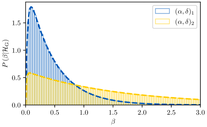
Figure 1: Noise distribution of coherent $\beta$ for $T_{\mathrm{seg}}=$900\text{\,}\mathrm{s}$$ (starting at GPS time $t_{0}=$1\,234\,567\,890\text{\,}\mathrm{s}$$, data from H1,L1), for two sky positions $(\alpha,\delta)_{1}=(5.16,0.78)\,$\mathrm{rad}$$, and $(\alpha,\delta)_{2}=(0.32,0.49)\,$\mathrm{rad}$$. The corresponding weights are $(w^{+},w^{\times})_{1}=(0.02,0.23)$ and $(w^{+},w^{\times})_{2}=(0.01,0.82)$, respectively. Dashed lines show the theoretical generalized $\tilde{\chi}^{2}$-distribution of (84), and the histograms are computed on $1\,000\,000$ synthesized values for $\beta$.

6.3 Coherent statistics

In Fig. 2 we present the same three coherent test cases used in [14], extended with the dominant-response $\mathcal{F}_{\mathrm{AB}}$-statistic (42) of [16], and the weak-signal Bayes-factor approximation $\beta$ of (50). All three cases use signals at fixed (relative) amplitude of $h_{*}=10$.

case (i) H1, $T_{\mathrm{seg}}=$25\text{\,}\mathrm{h}$$, $(\alpha,\delta)=(2,-0.5)\,$\mathrm{r}\mathrm{a}\mathrm{d}$$

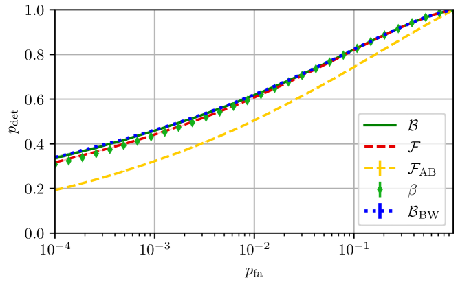
case (ii) H1, $T_{\mathrm{seg}}=$86\,164\text{\,}\mathrm{s}$$, $(\alpha,\delta)=(2,0)\,$\mathrm{r}\mathrm{a}\mathrm{d}$$

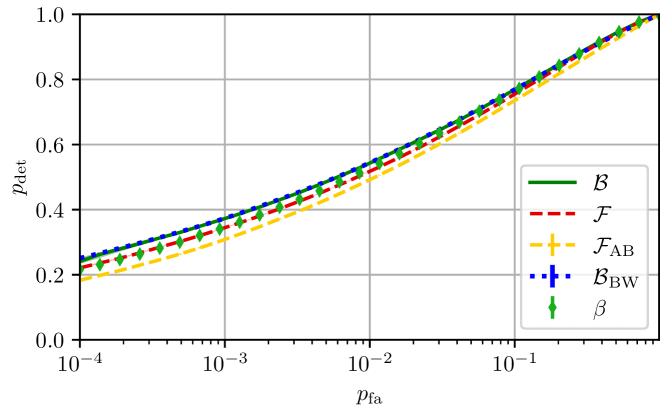
case (iii) H1+L1, $T_{\mathrm{seg}}=$100\text{\,}\mathrm{s}$$, $(\alpha,\delta)=(2,-0.5)\,$\mathrm{r}\mathrm{a}\mathrm{d}$$

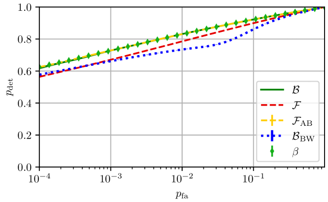
Figure 2: Detection probability as a function of false-alarm probability for the three different coherent test cases (i)-(iii) previously considered in [14]. In all cases the signal population has a fixed relative amplitude of $h_{*}=10$.

1. top panel: a coherent $T_{\mathrm{seg}}=$25\text{\,}\mathrm{h}$$ search on H1 data (starting at GPS time $756\,950\,413\text{\,}\mathrm{s}$) for sky-position $(\alpha,\delta)=(2,-0.5)\,$\mathrm{r}\mathrm{a}\mathrm{d}$$ (the original example from [8]). Here $\beta$ performs similarly to $\mathcal{F}$ and slightly worse than $\mathcal{B}{{}_{\mathrm{BW}}}$, which perfectly approximates the performance of $\mathcal{B}$. The dominant-response $\mathcal{F}_{\mathrm{AB}}$ performs worst as expected in this relatively long-segment case.

2. middle panel: a similar case with $T_{\mathrm{seg}}=$1\text{\,}\textrm{sidereal day}$$ ($86\,164\text{\,}\mathrm{s}$), same start-time as (i), for a single detector (H1) and sky-position at the equator $(\alpha,\delta)=(2,0)\,$\mathrm{r}\mathrm{a}\mathrm{d}$$, with qualitatively similar results case (i).

3. bottom panel: a short coherence length of $T_{\mathrm{seg}}=$100\text{\,}\mathrm{s}$$ for two detectors (H1 and L1), sky position $(\alpha,\delta)=(2,-0.5)\,$\mathrm{r}\mathrm{a}\mathrm{d}$$ at sidereal time $00:00$ (using GPS mid-time $756\,581\,823\text{\,}\mathrm{s}$). Here $\mathcal{B}{{}_{\mathrm{BW}}}$ performs worse or similar to $\mathcal{F}$ (reproducing the result of [14]), while both the dominant-response $\mathcal{F}_{\mathrm{AB}}$ as well as the weak-signal $\beta$-statistics perform as well as the full $\mathcal{B}$-statistic

6.4 Semi-coherent results

We consider semi-coherent searches with a fixed total duration of $T_{\mathrm{span}}=$10\text{\,}\mathrm{d}$$, with variable segment lengths spanning from a very short-segments at $T_{\mathrm{seg}}=$900\text{\,}\mathrm{s}$$ (with $N_{\mathrm{seg}}=960$ segments) to a fully-coherent search at $T_{\mathrm{span}}=$10\text{\,}\mathrm{d}$$. Here we ensure that all $N_{\mathrm{seg}}$ segments are of equal length $T_{\mathrm{seg}}$, in order to avoid confounding the results with the effect of varying data-factors shown and discussed in the next section.

The results of these simulations are shown in figure 3. We use a fixed false-alarm probability of $p_{\mathrm{fa}}=${10}^{-3}$$ and a sky position of $(\alpha,\delta)=(2,-0.5)\,$\mathrm{r}\mathrm{a}\mathrm{d}$$. Note that here we do not include a semi-coherent summed $\mathcal{B}$-statistic, as this requires numerical 2D integration for each sample and segment, making it impractical to obtain good sampling in a reasonable time. This is of course the same reason this statistic is not practical for any real searches in the first place.

The signal strength $h_{*}(T_{\mathrm{seg}})$ is determined for each $T_{\mathrm{seg}}$ by requiring a fixed detection probability of $p_{\mathrm{det}}(2\widehat{\mathcal{F}})=0.7$ for the standard semi-coherent $\widehat{\mathcal{F}}$-statistic, in order to operate in a relevant $p_{\mathrm{det}}$ range across all $T_{\mathrm{seg}}$ despite the greatly different sensitivities. This results in a range of $h_{*}(T_{\mathrm{seg}}=$900\text{\,}\mathrm{s}$)\sim 1.9$ to $h_{*}(T_{\mathrm{seg}}=$10\text{\,}\mathrm{d}$)\sim 13.9$ for the per-segment relative amplitude. As discussed in Sec. 4.5, even at the shortest segment length this relative signal amplitude does not fall into the “weak-signal” regime of $h_{*}\ll 1$.

The top panel in figure 3 shows the single-detector case for H1, the middle panel is for H1+L1 and bottom panel additionally includes Virgo V1, with qualitatively similar results in all three cases:

• the $\mathcal{B}{{}_{\mathrm{BW}}}$ approximation performs well at segment lengths $T_{\mathrm{seg}}\gtrsim$1\text{\,}\mathrm{d}$$, where it effectively equals the performance of the (weighted and unweighted) $\widehat{\mathcal{F}}$ statistics. This may seem surprising given Fig. 2, but at the larger $p_{\mathrm{det}}$ and $p_{\mathrm{fa}}$ values used here the differences become very small. As anticipated from the coherent results and the discussion in [14], $\mathcal{B}{{}_{\mathrm{BW}}}$ increasingly loses sensitivity at shorter segment lengths (and can run into similar numerical degeneracy issues with inverting $\mathcal{M}_{\mu\nu}$ (12) as the $\mathcal{F}$-statistic [16]).

• the dominant-response statistic $\widehat{\mathcal{F}}_{\mathrm{AB}}$ performs better than $\widehat{\mathcal{F}}$ at short $T_{\mathrm{seg}}$ and increasingly poorly at longer segments $T_{\mathrm{seg}}\gtrsim$19\text{\,}\mathrm{h}$$, as expected [16]. We can also confirm that the (empirical) weighting scheme (54) introduced in [17] further improves the short-segment performance, for both $\widehat{\mathcal{F}}_{\mathrm{w}}$ as well as $\widehat{\mathcal{F}}_{\mathrm{ABw}}$. This can be understood from the fact that the antenna-pattern sensitivity to a fixed sky position varies more strongly for short segments, which is where the segment weighting can gain more sensitivity.

  However, note that this Monte-Carlo simulation uses perfectly white Gaussian noise of constant noise floor and $100\text{\,}\mathrm{\char 37\relax}$ duty factor over all segments, which is why the contribution of the data factor $\gamma_{\ell}$ to the segment weights does not confer any benefits at longer segment durations $T_{\mathrm{seg}}\gtrsim$1\text{\,}\mathrm{d}$$ here, which will be discussed further in the next section.

• the semi-coherent weak-signal Bayes-factor approximation $\widehat{\beta}$ performs effectively “optimally” across both the short- and long-segment regimes, equalizing (and improving upon) the weighted dominant-response statistic $\widehat{\mathcal{F}}_{\mathrm{ABw}}$ at short segments, while converging to the $\widehat{\mathcal{F}}_{\mathrm{(w)}}$ and $\mathcal{B}{{}_{\mathrm{BW}}}$ performance at long segments (at least for equal-data-factor segments, see next section).

H1

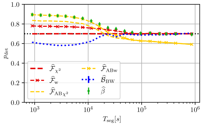
H1+L1

H1+L1+V1

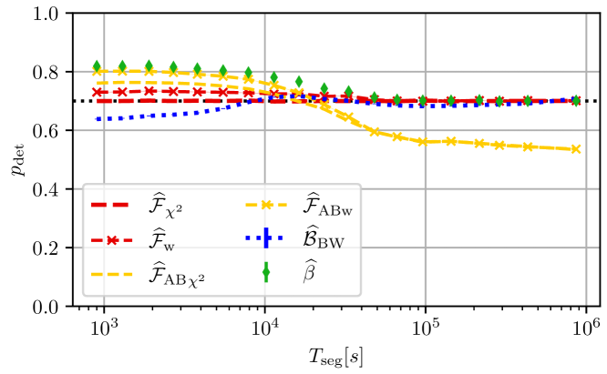
Figure 3: Detection probability as a function of semi-coherent segment length $T_{\mathrm{seg}}$ at fixed total span of $T_{\mathrm{span}}=$10\text{\,}\mathrm{d}$$ (with GPS start time $756\,950\,413\text{\,}\mathrm{s}$), false-alarm probability $p_{\mathrm{fa}}=${10}^{-3}$$ and sky position $(\alpha,\delta)=(2,-0.5)\,$\mathrm{r}\mathrm{a}\mathrm{d}$$. The top panel is for a single detector (H1), middle panel is H1+L1 and bottom panel includes Virgo H1+L1+V1. The relative signal amplitude $h_{*}(T_{\mathrm{seg}})$ is adjusted for a fixed detection probability $p_{\mathrm{det}}(2\widehat{\mathcal{F}})=0.7$ for the standard semi-coherent $\widehat{\mathcal{F}}$-statistic.

6.5 Performance for unequal data-factors $\gamma_{\ell}$

The per-segment weights of various semi-coherent weighted statistics $\widehat{\mathcal{F}}_{\mathrm{w}}$, $\widehat{\mathcal{F}}_{\mathrm{ABw}}$, as well as the weak-signal Bayes-factor approximation $\widehat{\beta}$ are a combination of an antenna-pattern- and a data-factor weight contribution, see section 4.4.

The semi-coherent Monte-Carlo simulations in the previous section use ideal segments with equal noise-floors and data amounts, and therefore equal per-segment data factors $\gamma_{\ell}$. Given that for segments longer than a day the antenna-pattern weight contributions also become increasingly constant, this explains why the weighted statistics $\widehat{\mathcal{F}}_{\mathrm{w}}$, $\widehat{\mathcal{F}}_{\mathrm{ABw}}$ and $\widehat{\beta}$ do not confer any benefits over the unweighted version in that case, as seen in figure 3.

As a proof of principle we now consider a rather extreme example of a semi-coherent search with three segments of $T_{\mathrm{seg}}=$25\text{\,}\mathrm{h}$$ with widely different duty factors of $0.1$, $1$ and $1$, respectively, resulting in the same relative variation of per-segment data factors $\gamma_{\ell}$. The result is shown in figure 4, illustrating that the weighted statistics $\widehat{\mathcal{F}}_{\mathrm{w}}$ and $\widehat{\beta}$ now do outperform both $\widehat{\mathcal{F}}$ and $\mathcal{B}{{}_{\mathrm{BW}}}$, as well as (maybe somewhat surprisingly) the full $\mathcal{B}$-statistic.

This result seems to strongly suggest that it is specifically the weak-signal (half-Gaussian) prior of (43) (but also (86)) that yields the right per-segment weighting, while the strong-signal limit $\mathcal{B}$-statistic (and its approximation $\mathcal{B}{{}_{\mathrm{BW}}}$) intrinsically lack this feature.

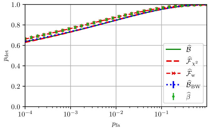
Figure 4: Detection probability as a function of false-alarm probability for a semi-coherent search on three unequal-$\gamma_{\ell}$ segments of $T_{\mathrm{seg}}=$25\text{\,}\mathrm{h}$$, with per-segment duty factors of $0.1$, $1$ and $1$, respectively, assuming two detectors H1 and L1. The signal sky-position is $(\alpha,\delta)=(2,-0.5)$ and the relative amplitude is fixed at $h_{*}=10$.

7 Conclusions

In this paper we have generalized the Bayesian $\mathcal{B}$-statistic by using a half-Gaussian $h_{0}$-prior instead of a uniform prior. This reduces to the $\mathcal{B}$-statistic in the strong-signal limit ($H\rightarrow\infty$) but yields a new analytic approximation in the weak-signal limit ($H\rightarrow 0$), defining the new weak-signal statistic $\beta(x)$. This statistic is shown to follow a generalized $\tilde{\chi}^{2}$-distribution with $(2,2)$ degrees of freedom per segment, with weights determined by the eigenvalues of the detector-response matrix $\mathcal{M}_{\mu\nu}$ and non-centrality parameters given by the corresponding signal-power components.

The sensitivity of $\beta$ is found to be comparable to $\mathcal{F}$ for day-long coherent searches, making it slightly less sensitive than the $\mathcal{B}$-statistic (and the Bero-Whelan approximation). However, for semi-coherent searches, it matches or outperforms both (i) the best short-segment statistic (i.e., the weighted dominant-response statistic $\widehat{\mathcal{F}}_{\mathrm{ABw}}$), and (ii) the best practical long-segment statistic, i.e., the weighted $\widehat{\mathcal{F}}_{\mathrm{w}}$-statistic.

Overall, the weak-signal $\beta$-statistic appears to be a powerful and practical detection statistic across a wide range of segment lengths that we have tested, namely from $900\text{\,}\mathrm{s}$ to $10\text{\,}\mathrm{d}\mathrm{a}\mathrm{y}\mathrm{s}$. Further testing is needed across various real-world scenarios and different false-alarm regimes beyond those considered here.

One interesting practical question is how to correctly perform an all-sky search with a statistic (such as $\beta$) that has a sky-position-dependent false-alarm distribution. This issue is not new and already affects any antenna-pattern-weighted segment statistics. A common practical solution is to use a “noise-normalized” critical-ratio statistic for the candidate ranking.

Another potentially interesting application of this new statistic is the line-robust framework of [25, 26]. The prior scaling parameter $H$, which governs the new Bayes factor, has a more direct physical interpretation compared to the unphysical prior cutoff parameter in the $\mathcal{F}$-statistic-prior, which complicates the correct tuning of the line-robust $B_{\mathrm{S/GL}}$ statistics.

Appendix A Alternative derivation of $\beta$ from weak-signal $\mathcal{F}$-statistic prior

Similar to the idea of using a (half-) Gaussian $h_{0}$-prior (43), we can use a Gaussian $\mathcal{A}^{\mu}$ prior centered on zero with scale $H$, namely

$$P\left(\mathcal{A}|\mathcal{H}_{\mathrm{S}}\right)=\frac{1}{(2\pi)^{2}H^{4}}e^{-\frac{1}{2}\mathcal{A}^{\mu}C_{\mu\nu}\mathcal{A}^{\nu}}\quad\text{with}\quad C_{\mu\nu}\equiv\frac{1}{H^{2}}\delta_{\mu\nu}\,,$$ (86)

which reduces to the original uniform-$\mathcal{A}^{\mu}$ $\mathcal{F}$-statistic prior of Sec. 3.2 in the strong-signal limit $H\rightarrow\infty$. This prior preserves the functional form of the likelihood ratio (7) and we can write the resulting Bayes-factor integral in analogy to (16) as

$$B_{\mathrm{{\mathrm{S}}/{\mathrm{G}}}}(x)=\frac{1}{\sqrt{\det\mathcal{M}_{\mathrm{H}}}}e^{\mathcal{F}_{\mathrm{H}}(x)}\,,$$ (87)

with modified detector-response matrix

$$\mathcal{M}_{\mathrm{H}}{}_{\mu\nu}\equiv\mathcal{M}_{\mu\nu}-\frac{1}{H^{2}}\delta_{\mu\nu}=\gamma\left(\begin{array}[]{cc}m_{\mathrm{H}}&0\\ 0&m_{\mathrm{H}}\end{array}\right),$$ (88)

where

$$m_{\mathrm{H}}\equiv\left(\begin{array}[]{cc}A-\frac{1}{\gamma H^{2}}&C\\ C&B-\frac{1}{\gamma H^{2}}\end{array}\right)$$ (89)

and we defined the modified $\mathcal{F}_{\mathrm{H}}$-statistic as

$$2\mathcal{F}_{\mathrm{H}}(x)\equiv x_{\mu}\left(\mathcal{M}_{\mathrm{H}}^{-1}\right)^{\mu\nu}x_{\nu}\,.$$ (90)

Considering $\det\mathcal{M}_{\mathrm{H}}=\gamma^{4}D_{\mathrm{H}}^{2}$ with the sub-determinant

$$D_{\mathrm{H}}\equiv\det m_{\mathrm{H}}=D-\frac{A+B}{\gamma H^{2}}+\frac{1}{\gamma^{2}H^{4}}\,,$$ (91)

in the weak-signal limit $H_{*}^{2}\ll 1$ we obtain the limiting expressions $D_{\mathrm{H}}\binrel@{\longrightarrow}\binrel@@{\mathop{\kern 0.0pt\longrightarrow}\limits^{{}H\rightarrow 0}}\frac{1}{\gamma^{2}{}H^{4}}$, $\mathcal{M}_{\mathrm{H}}\rightarrow\frac{1}{{}H^{2}}\mathbb{I}$, and $\sqrt{\det\mathcal{M}_{\mathrm{H}}}\rightarrow H^{-4}$, and finally

$$2\mathcal{F}_{\mathrm{H}}(x)\binrel@{\longrightarrow}\binrel@@{\mathop{\kern 0.0pt\longrightarrow}\limits^{{}H\rightarrow 0}}\gamma{}H^{2}\beta(x),$$ (92)

which yields the resulting Bayes factor as

$$B_{\mathrm{S/G}}\rightarrow H^{4}e^{H_{*}^{2}\,\beta(x)}\,,$$ (93)

in terms of the weak-signal $\beta$-statistic of (50). While normalized differently, this is otherwise equivalent to the weak-signal Bayes factor obtained in (52).

Appendix B General matched-filter scalar product $\left(x|y\right)$

The scalar product $\left(x|y\right)$ of (5) can be fully generalized [18, 9] to several detectors $X=1,\ldots,N_{\mathrm{d}}$, each providing a finite set of data chunks (commonly referred to as short Fourier transforms or SFTs) $\alpha=1,\ldots,N_{\mathrm{sft}}^{X}$, each of length $T_{\mathrm{sft}}$, allowing for gaps in between SFTs and for individual noise-floors $\mathcal{S}_{X\alpha}$ (assumed stationarity only during each SFT). This results in the general form for the scalar product

$$\left(x|y\right)=2\gamma\,\langle{x\,y}\rangle,\quad\text{with}\quad\gamma\equiv\mathcal{S}^{-1}\,T_{\mathrm{data}},$$ (94)

where the dimensionless data factor [16] $\gamma$ is defined in terms of the overall noise-floor $\mathcal{S}$ and total amount of data $T_{\mathrm{data}}$, namely

$$\mathcal{S}^{-1}\equiv\frac{1}{N_{\mathrm{sft}}}\sum_{X\alpha}\mathcal{S}_{X\alpha}^{-1}\,,\qquad T_{\mathrm{data}}\equiv N_{\mathrm{sft}}\,T_{\mathrm{sft}}\,,$$ (95)

and $N_{\mathrm{sft}}\equiv\sum_{X}N_{\mathrm{sft}}^{X}$. The weighted multi-detector average can be written as

$$\langle{x\,y}\rangle\equiv\frac{1}{N_{\mathrm{sft}}}\sum_{X\alpha}w_{X\alpha}\,\frac{1}{T_{\mathrm{sft}}}\int_{0}^{T_{\mathrm{sft}}}x_{X\alpha}(t)\,y_{X\alpha}(t)\,dt,$$ (96)

where $x_{X\alpha}$ refers to the data chunk $\alpha$ from detector $X$, and the corresponding noise weights are defined as $w_{X\alpha}\equiv\mathcal{S}^{-1}_{X\alpha}/\mathcal{S}^{-1}$, such that $\sum_{X\alpha}w_{X\alpha}=N_{\mathrm{sft}}$.

Appendix C Matched filter in physical coordinates

Expressing the scalar-product “match term” $\left(x|h\right)=\mathcal{A}^{\mu}x_{\mu}$ of (4) in physical amplitude coordinates $\{h_{0},\eta,\psi,\phi_{0}\}$ yields (after some tedious but straightforward algebra):

$$\eqalign{\left(x|h\right)&=\mathcal{A}^{\mu}x_{\mu}=Q_{\mathrm{s}}\,\sin\phi_{0}+Q_{\mathrm{c}}\,\cos\phi_{0}\\ &=Q(x;h_{0},\eta,\psi)\,\cos\left(\phi_{0}-\varphi_{0}\right)\,,}$$ (97)

with

$$\eqalign{Q_{\mathrm{s}}&\equiv-\sin 2\psi\left(x_{1}\,A_{\times}+x_{4}\,A_{+}\right)+\cos 2\psi\left(x_{2}\,A_{\times}-x_{3}\,A_{+}\right)\,,\\ Q_{\mathrm{c}}&\equiv\hskip 10.00002pt\sin 2\psi\left(x_{2}\,A_{+}-x_{3}\,A_{\times}\right)+\cos 2\psi\left(x_{1}\,A_{+}+x_{4}\,A_{\times}\right)\,,}$$ (98)

where $A_{+}\equiv h_{0}\,(1+\eta^{2})/2$ and $A_{\times}\equiv h_{0}\,\eta$, and where we defined

$$\eqalign{Q^{2}&\equiv Q_{\mathrm{s}}^{2}+Q_{\mathrm{c}}^{2}=h_{*}^{2}q^{2}\,,\\ \tan\varphi_{0}&\equiv{Q_{\mathrm{s}}}/{Q_{\mathrm{c}}},}$$ (99)

which was used to write the likelihood ratio in the form (20).

References

References

- [1] Collaboration T L S, Aasi J et al. 2015 Classical and Quantum Gravity 32 074001 ISSN 0264-9381 publisher: IOP Publishing URL https://dx.doi.org/10.1088/0264-9381/32/7/074001
- [2] Acernese F et al. 2014 Classical and Quantum Gravity 32 024001 ISSN 0264-9381 publisher: IOP Publishing URL https://dx.doi.org/10.1088/0264-9381/32/2/024001
- [3] Riles K 2023 Living Reviews in Relativity 26 3 ISSN 1433-8351 number: 1 URL https://doi.org/10.1007/s41114-023-00044-3
- [4] Wette K 2023 Astroparticle Physics 153 102880 ISSN 0927-6505 URL https://www.sciencedirect.com/science/article/pii/S092765052300066X
- [5] Jaranowski P, Królak A and Schutz B F 1998 58 063001
- [6] Astone P, D’Antonio S, Frasca S and Palomba C 2010 Classical and Quantum Gravity 27 194016 ISSN 0264-9381 number: 19 URL https://ui.adsabs.harvard.edu/abs/2010CQGra..27s4016A/abstract
- [7] Searle A C 2008 ArXiv E-Prints _eprint: 0804.1161 URL http://adsabs.harvard.edu/abs/2008arXiv0804.1161S
- [8] Prix R and Krishnan B 2009 26 204013
- [9] Whelan J T, Prix R, Cutler C J and Willis J L 2014 Classical and Quantum Gravity 31 065002
- [10] Dergachev V 2012 \prd 85 062003 _eprint: 1110.3297 URL http://adsabs.harvard.edu/abs/2012PhRvD..85f2003D
- [11] Haris K and Pai A 2017 Physical Review D 96 102002 publisher: American Physical Society URL https://link.aps.org/doi/10.1103/PhysRevD.96.102002
- [12] Dhurandhar S, Krishnan B and Willis J L 2017 Marginalizing the likelihood function for modeled gravitational wave searches publication Title: arXiv e-prints ADS Bibcode: 2017arXiv170708163D Type: article URL https://ui.adsabs.harvard.edu/abs/2017arXiv170708163D
- [13] Wette K 2021 Universe 7 174 ISSN 2218-1997 URL https://ui.adsabs.harvard.edu/abs/2021Univ....7..174W
- [14] Bero J J and Whelan J T 2018 Classical and Quantum Gravity 36 015013 ISSN 0264-9381
- [15] Covas P B, Papa M A, Prix R and Owen B J 2022 arXiv:2203.01773 Submitted to ApJL URL https://ui.adsabs.harvard.edu/abs/2022arXiv220301773C
- [16] Covas P B and Prix R 2022 Improved short-segment detection statistic for continuous gravitational waves publication Title: arXiv e-prints ADS Bibcode: 2022arXiv220308723C Type: article URL https://ui.adsabs.harvard.edu/abs/2022arXiv220308723C
- [17] Covas P and Prix R 2022 Physical Review D 106 084035 number: 8 Publisher: American Physical Society URL https://ui.adsabs.harvard.edu/abs/2022arXiv220801543C
- [18] Prix R 2010 The -statistic and its implementation in ComputeFstatistic_v2 Tech. rep. LIGO DCC (LIGO-T0900149-v6) URL https://dcc.ligo.org/LIGO-T0900149/public
- [19] Stuart A, Ord J K and Arnold S 1999 Kendall’s advanced theory of statistics. Vol.2A: Classical inference and the linear model (Arnold) publication Title: Kendall’s Advanced Theory of Statistics. Vol.2A: Classical Inference and the Linear Model, 6th Ed., by A. Stuart, J.K. Ord, and S. Arnold. 3 Volumes London: Hodder Arnold, 1999
- [20] Finn L S 1992 Physical Review D 46 5236–5249 publisher: American Physical Society URL https://link.aps.org/doi/10.1103/PhysRevD.46.5236
- [21] Jaynes E T 2003 Probability Theory. The Logic of Science (Cambridge University Press)
- [22] Searle A C, Sutton P J, Tinto M and Woan G 2008 Classical and Quantum Gravity 25 114038 ISSN 0264-9381 URL https://dx.doi.org/10.1088/0264-9381/25/11/114038
- [23] Searle A C, Sutton P J and Tinto M 2009 Classical and Quantum Gravity 26 155017 ISSN 0264-9381 URL https://dx.doi.org/10.1088/0264-9381/26/15/155017
- [24] Prix R, Giampanis S and Messenger C 2011 Physical Review D 84 023007 ISSN 1550-79980556-2821 aDS Bibcode: 2011PhRvD..84b3007P URL https://ui.adsabs.harvard.edu/abs/2011PhRvD..84b3007P
- [25] Keitel D, Prix R, Papa M A, Leaci P and Siddiqi M 2014 Physical Review D 89 064023 ISSN 1550-79980556-2821 aDS Bibcode: 2014PhRvD..89f4023K URL https://ui.adsabs.harvard.edu/abs/2014PhRvD..89f4023K
- [26] Keitel D 2016 Physical Review D 93 084024 publisher: American Physical Society URL https://link.aps.org/doi/10.1103/PhysRevD.93.084024
- [27] Wette K 2012 85 042003 (Preprint DCCLIGO-P1100151-v2) URL https://dcc.ligo.org/cgi-bin/private/DocDB/ShowDocument?docid=75488
- [28] Dreissigacker C, Prix R and Wette K 2018 98 084058 (Preprint 1808.02459)
- [29] Abramowitz M and Stegun I A 1964 Handbook of Mathematical Functions (National Bureau of Standards)
- [30] Confluent hypergeometric function: Asymptotic behavior https://en.wikipedia.org/wiki/Confluent_hypergeometric_function#Asymptotic_behavior accessed: 2024-09-05
- [31] Astone P, Colla A, D’Antonio S, Frasca S, Palomba C and Serafinelli R 2014 Physical Review D 89 062008 publisher: American Physical Society URL https://link.aps.org/doi/10.1103/PhysRevD.89.062008
- [32] D’Onofrio L, Astone P, Pra S D, D’Antonio S, Di Giovanni M, De Rosa R, Leaci P, Mastrogiovanni S, Mirasola L, Muciaccia F, Palomba C and Pierini L 2024 Two sides of the same coin: the F-statistic and the 5-vector method arXiv:2406.09236 [gr-qc] URL http://arxiv.org/abs/2406.09236
- [33] Collaboration L S 2004 Physical Review D 69 082004 URL https://ui.adsabs.harvard.edu/abs/2004PhRvD..69h2004A/abstract
- [34] Davies R B 1980 Journal of the Royal Statistical Society: Series C (Applied Statistics) 29 323–333 ISSN 1467-9876 _eprint: https://onlinelibrary.wiley.com/doi/pdf/10.2307/2346911 URL https://onlinelibrary.wiley.com/doi/abs/10.2307/2346911
- [35] Das A and Geisler W S 2021 arXiv:2012.14331 [cs, stat] ArXiv: 2012.14331 URL http://arxiv.org/abs/2012.14331
- [36] 2024 Generalized chi-squared distribution page Version ID: 1230476684 URL https://en.wikipedia.org/w/index.php?title=Generalized_chi-squared_distribution&oldid=1230476684
- [37] Hammarwall D, Bengtsson M and Ottersten B 2008 IEEE Transactions on Signal Processing 56 1188–1204 ISSN 1941-0476 number: 3 Conference Name: IEEE Transactions on Signal Processing URL https://ieeexplore.ieee.org/document/4451286