Inverse Differential Riccati Equation to Optimized Human-Robot Collaboration

Abstract

This paper presents a framework for human-robot collaboration that integrates optimal trajectory generation with a robust tracking control strategy. The proposed framework leverages the inverse differential Riccati equation to optimize the collaboration dynamics, providing an efficient method to generate time-varying, task-specific trajectories for the human-robot system. To ensure the accurate tracking of these trajectories, a neuro-adaptive PID control method is implemented, capable of compensating for system uncertainties and variations. This control strategy dynamically adjusts the PID gains using a radial basis function neural network, ensuring both stability and adaptability. Simulations demonstrate the method’s effectiveness in achieving optimized human-robot collaboration and accurate joint-space tracking, making it suitable for real-world applications.

I Introduction

Human-robot collaboration (HRC) is becoming increasingly important across fields like manufacturing, healthcare, and service industries, where robots must work alongside humans in dynamic and uncertain environments. In these scenarios, robots need control systems that balance precision and adaptability [10]. Traditional control methods, which rely on predefined trajectories, often limit a robot’s ability to adapt to human input in real time. This limitation drives the need for more flexible control frameworks capable of dynamic adjustment during interaction [15].

Impedance control has been widely used to regulate interaction forces between humans and robots, ensuring safe and compliant collaboration [11]. While effective, most existing approaches use fixed impedance models that assume static behavior, which doesn’t fully capture the changing dynamics of real-world collaboration [17]. Additionally, control strategies that rely on predefined trajectories reduce the robot’s capacity to adapt to evolving human input or task changes during collaboration [12].

Recent work has explored adaptive and learning-based approaches to address the variability in human behavior. Adaptive impedance control, reinforcement learning, and neural networks have been applied to improve real-time robot response [16, 13, 14]. However, these methods are often combined with computationally demanding control schemes or lack stability guarantees, limiting their use in real-time applications.

This paper proposes a task-specific control framework for human-robot collaboration that eliminates the need for a predefined desired trajectory. Moreover, it employs time-varying impedance parameters for both the human and robot impedance models, capturing the adaptive nature of human control during interaction. To optimize the collaboration, the framework leverages the inverse Differential Riccati Equation (iDRE) to generate optimal control trajectories, enhancing collaboration performance. Additionally, a low-computational neuro-adaptive PID control strategy is introduced to ensure stability and precise joint-space tracking. By dynamically adjusting PID gains in real time, the control law effectively handles uncertainties and varying human inputs, offering both computational efficiency and robust performance for real-time applications.

In summary, the main contributions of this paper are: (1) the development of a task-specific HRC framework that optimizes collaboration using iDRE without requiring a predefined trajectory, (2) the incorporation of time-varying impedance parameters for both human and robot models, reflecting the adaptive nature of human control strategies, and (3) the design of a neuro-adaptive PID controller that ensures accurate joint-space tracking with minimal computational overhead.

The remainder of the paper is organized as follows: Section II introduces the system dynamics and problem formulation, Section III describes the iDRE-based optimization for human-robot collaboration, Section IV details the neuro-adaptive PID control design, and Section V presents the simulation results that validate the proposed framework. Finally, conclusions and future work are discussed in Section VI.

II Problem Formulation

II-A System Description

The robot’s kinematics in task space are described by:

$$x=\Phi(q),$$ (1)

where $q(t)\in\mathbb{R}^{n}$ is the vector of generalized joint coordinates, and $x(t)\in\mathbb{R}^{n_{e}}$ represents the Cartesian position of the end-effector, with $n$ being the number of joints and $n_{e}$ the dimension of the task space.

The robot dynamics in the joint space are expressed as:

$$\mathbf{M_{r}}(q)\ddot{q}(t)+\mathbf{C_{r}}(q,\dot{q})\dot{q}(t)+\mathbf{G_{r}}(q)=\tau(t)+\mathbf{J}^{T}(q)f_{h}(t),$$ (2)

where $\mathbf{M_{r}}(q)\in\mathbb{R}^{n\times n}$ is the positive-definite mass matrix, $\mathbf{C_{r}}(q,\dot{q})\in\mathbb{R}^{n}$ represents the Coriolis and centrifugal forces, $\mathbf{G_{r}}(q)\in\mathbb{R}^{n}$ is the gravitational force, and $\mathbf{J}(q)\in\mathbb{R}^{n_{e}\times n}$ is the Jacobian matrix. The input torque is $\tau(t)\in\mathbb{R}^{n}$, and $f_{h}(t)$ is the human-applied force.

By transforming the joint-space dynamics (2) into Cartesian space using $\dot{x}(t)=\mathbf{J}(q)\dot{q}(t)$ and $\ddot{x}(t)=\dot{\mathbf{J}}(q)\dot{q}(t)+\mathbf{J}(q)\ddot{q}(t)$, the Cartesian-space robot dynamics become:

$$\mathbf{M_{c}}(q)\ddot{x}(t)+\mathbf{C_{c}}(q,\dot{q})\dot{x}(t)+\mathbf{G_{c}}(q)=u(t)+u_{h}(t),$$ (3)

where $\mathbf{M_{c}}(q)=\mathbf{J}^{-T}(q)\mathbf{M_{r}}(q)\mathbf{J}^{-1}(q)$, $\mathbf{C_{c}}(q,\dot{q})=\mathbf{J}^{-T}(q)\left(\mathbf{C_{r}}(q,\dot{q})-\mathbf{M_{r}}(q)\mathbf{J}^{-1}(q)\dot{\mathbf{J}}(q)\right)\mathbf{J}^{-1}(q)$, $\mathbf{G_{c}}(q)=\mathbf{J}^{-T}(q)\mathbf{G_{r}}(q)$, $u(t)=\mathbf{J}^{-T}(q)\tau(t)$, and $u_{h}(t)=f_{h}(t)$.

To guide the interaction, we employ an impedance model that defines the desired behavior of the system:

$$\mathbf{M_{\text{imp}}}(t)\ddot{x}_{\text{imp}}(t)+\mathbf{B_{\text{imp}}}(t)\dot{x}_{\text{imp}}(t)+\mathbf{K_{\text{imp}}}(t)x_{\text{imp}}(t)=f_{h}(t),$$ (4)

where $\mathbf{M_{\text{imp}}}(t)$, $\mathbf{B_{\text{imp}}}(t)$, and $\mathbf{K_{\text{imp}}}(t)$ are the time-varying impedance parameters: mass, damping, and stiffness, respectively. $x_{\text{imp}}(t)$ represents the output of the prescribed impedance model. The impedance model is designed to regulate the interaction forces, ensuring smooth collaboration between the human and the robot by modulating the system’s response to applied forces.

The human impedance model describes the human-applied force $f_{h}(t)$ in response to the robot’s motion. The model can be expressed as:

$$\left(\mathbf{K_{d}}(t)s+\mathbf{K_{p}}(t)\right)f_{h}(t)=\mathbf{k_{e}}(t)x_{d}(t),$$ (5)

where $s$ is the Laplace operator. $\mathbf{K_{d}}(t)$ and $\mathbf{K_{p}}(t)$ represent time-varying human damping and stiffness gains, respectively. $\mathbf{k_{e}}(t)$ is the human control gain, and $x_{d}(t)$ is the desired human trajectory. This model reflects the adaptive nature of human control during interaction.

Property 1 [2], [4]. The mass matrix $\mathbf{M_{c}}(q)$ is symmetric, positive definite, and its norm is bounded by constants $\alpha_{m}>0$ and $\alpha_{M}>0$, such that $\alpha_{m}\leq\|\mathbf{M_{c}}(q)\|\leq\alpha_{M}$.

Property 2 [4], [3]. The matrix $\dot{\mathbf{M_{c}}}(q)-2\mathbf{C_{c}}(q,\dot{q})$ is skew-symmetric, i.e., for any vector $\lambda\in\mathbb{R}^{n}$, $\lambda^{T}\left(\dot{\mathbf{M_{c}}}(q)-2\mathbf{C_{c}}(q,\dot{q})\right)\lambda=0$. Furthermore, there exist constants $\eta>0$ and $\delta>0$, such that $\|\mathbf{C_{c}}(q,\dot{q})\|\leq\eta\|\dot{q}(t)\|$ and $\|\mathbf{G_{c}}(q)\|\leq\delta$.

II-B Problem Statement

This paper focuses on optimizing human-robot collaboration by combining the robot dynamics, impedance control, and human interaction models. The robot follows an impedance-based behavior that adapts to the forces applied by the human. The human’s control efforts are modeled with time-varying gains, capturing the adaptive nature of human behavior during interaction. The goal is to optimize the system’s performance by minimizing the interaction forces and ensuring smooth collaboration, without a predefined trajectory. Additionally, a simple yet effective control strategy is designed to ensure accurate tracking of the generated trajectories, compensating for uncertainties and maintaining stability throughout the interaction. A simple yet effective control strategy is designed to ensure accurate tracking of the generated trajectories, compensating for uncertainties while maintaining stability throughout the interaction.

III Task-Specific Assistive Human-Robot Collaboration

This section focuses on developing an optimized interaction framework between a robot and a human collaborator. By unifying the human impedance model and the robot’s compliant behavior, we derive a task-specific collaboration model that effectively captures human-robot interaction dynamics. iDRE is applied to optimize the system’s trajectory and performance.

III-A Optimal Collaboration using iDRE

We start by presenting the iDRE method, which will later be used to optimize the human-robot collaboration dynamics. This method allows us to compute an optimal control trajectory over a given time horizon based on a system’s state equation:

$$\dot{X}(t)=\mathbf{A}(t)X(t)+\mathbf{B}(t)u(t),$$ (6)

where $X(t)\in\mathbb{R}^{n}$ is the state vector and $u(t)\in\mathbb{R}^{m}$ is the control input. The matrices $\mathbf{A}(t)\in\mathbb{R}^{n\times n}$ and $\mathbf{B}(t)\in\mathbb{R}^{n\times m}$ represent the system and input dynamics, which will be explained in detail in the next subsection. The boundary conditions for this system can be non-zero and are defined as:

$$X(t_{0})=X_{0},\quad X(t_{f})=X_{f}.$$ (7)

The objective is to minimize the following cost function:

$$\begin{split}E=\frac{1}{2}\int_{t_{0}}^{t_{f}}&\left(X^{T}(t)\mathbf{Q}(t)X(t)+2X^{T}(t)\mathbf{S}(t)u(t)\right.\\ &\left.+u^{T}(t)\mathbf{R}(t)u(t)\right)dt,\end{split}$$ (8)

where $\mathbf{Q}(t)\in\mathbb{R}^{n\times n}$, $\mathbf{S}(t)\in\mathbb{R}^{n\times m}$, and $\mathbf{R}(t)\in\mathbb{R}^{m\times m}$ are weight matrices, with $\mathbf{Q}(t)\geq 0$, $\mathbf{S}(t)\geq 0$, and $\mathbf{R}(t)>0$.

The optimal control input that minimizes this cost function is given by:

$$\begin{split}u^{*}(t)=&-\mathbf{R}^{-1}(t)\left(\mathbf{S}^{T}(t)+\mathbf{B}(t)^{T}\mathbf{P}^{-1}(t)\right)X^{*}(t)\\ &+\mathbf{R}^{-1}(t)\mathbf{B}(t)^{T}\mathbf{P}^{-1}(t)V(t),\end{split}$$ (9)

where $\mathbf{P}(t)$ and $V(t)$ are solutions to the inverse matrix differential Riccati equation:

$$\begin{split}\dot{\mathbf{P}}(t)=&\mathbf{A}(t)\mathbf{P}(t)+\mathbf{P}(t)\mathbf{A}(t)^{T}+\mathbf{P}(t)\mathbf{Q}(t)\mathbf{P}(t)\\ &-\left[\mathbf{P}(t)\mathbf{S}(t)+\mathbf{B}(t)\right]\mathbf{R}^{-1}(t)\left[\mathbf{S}^{T}(t)\mathbf{P}(t)+\mathbf{B}(t)^{T}\right],\end{split}$$ (10)

and the vector differential equation for $V(t)$:

$$\begin{split}\dot{V}(t)=&\left(\mathbf{A}(t)-\mathbf{B}(t)\mathbf{R}^{-1}(t)\mathbf{S}^{T}(t)+\mathbf{P}(t)\mathbf{Q}(t)\right.\\ &\left.-\mathbf{P}(t)\mathbf{S}(t)\mathbf{R}^{-1}(t)\mathbf{S}^{T}(t)\right)V(t).\end{split}$$ (11)

The set of equations (10) and (11) can be solved using either the initial or final boundary conditions:

$$t=t_{0}: \quad\mathbf{P}(t_{0})=0,\quad V(t_{0})=X(t_{0}),$$ (12)

$$t=t_{f}: \quad\mathbf{P}(t_{f})=0,\quad V(t_{f})=X(t_{f}).$$

For further details on the full development of iDRE and its advantages, refer to [5].

Remark 1: iDRE allows trajectory planning with non-zero initial and final points, making it well-suited for assistive tasks in human-robot collaboration where the desired states at both ends are predefined.

Remark 1: In contrast to conventional optimal control methods like Pontryagin’s maximum principle [6], which requires solving a complex two-point boundary value problem involving states and co-states, iDRE simplifies the process and avoids these difficulties, enabling more efficient solutions.

Remark 3: The presented method is time-varying and leads to closed-loop optimal control. This makes it easier to implement in real-world control systems, as the method adapts in real-time to changes during interaction.

III-B Unified System Dynamics

In this subsection, we define the unified system dynamics that capture the interaction between the human and the robot through an impedance model. The dynamics formulated here will be used in conjunction with the iDRE optimization presented earlier. By modeling the time-varying human impedance and the robot’s desired behavior, we create a unified system that can be optimized to enhance collaboration without relying on predefined trajectories.

To model the human-robot interaction, we start by describing the human-generated force, which is time-varying and adaptive to the robot’s motion. The human impedance model (5) can be rewritten in the time domain as:

$$\mathbf{K_{d}}(t)\dot{f}_{h}(t)+\mathbf{K_{p}}(t)f_{h}(t)=\mathbf{k_{e}}(t)x_{d}(t).$$ (13)

This can be equivalently rewritten as:

$$\dot{f}_{h}(t)=\mathbf{A_{h}}(t)X_{d}(t)+\mathbf{B_{h}}(t)f_{h}(t),$$ (14)

where $\mathbf{A_{h}}(t)=\mathbf{k_{e}(t)}\mathbf{K}_{d1}(t)$, and $\mathbf{B_{h}}(t)=-\mathbf{K_{d}}(t)^{-1}\mathbf{K_{p}}(t)$, with $\mathbf{K}_{d1}(t)=\begin{bmatrix}\mathbf{K_{d}}(t)^{-1}&0\end{bmatrix}$, and $X_{d}(t)=\begin{bmatrix}x_{d}(t)^{T}&\dot{x}_{d}(t)^{T}\end{bmatrix}^{T}$.

Now, define the impedance state vector $\xi(t)=\begin{bmatrix}x_{\text{imp}}(t)^{T}&\dot{x}_{\text{imp}}(t)^{T}\end{bmatrix}^{T}$, where $x_{\text{imp}}(t)$ and $\dot{x}_{\text{imp}}(t)$ represent the desired position and velocity of the impedance behavior. The impedance model (4) can then be expressed as:

$$\dot{\xi}(t)=\mathbf{A_{\xi}}(t)\xi(t)+\mathbf{B_{\xi}}(t)u(t),$$ (15)

where $u(t)=\mathbf{M_{\text{imp}}}(t)^{-1}f_{h}(t)$, and the system matrices $\mathbf{A_{\xi}}(t)$ and $\mathbf{B_{\xi}}(t)$ are defined as: $\mathbf{A_{\xi}}(t)=\begin{bmatrix}0&\mathbf{I}_{n\times n}\\ -\mathbf{M_{\text{imp}}}(t)^{-1}\mathbf{K_{\text{imp}}}(t)&-\mathbf{M_{\text{imp}}}(t)^{-1}\mathbf{B_{\text{imp}}}(t)\end{bmatrix}$, and $\quad\mathbf{B_{\xi}}(t)=\begin{bmatrix}0\\ \mathbf{I}_{n\times n}\end{bmatrix}.$

It is important to note that the human’s desired trajectory $x_{d}(t)$ coincides with the reference trajectory of the impedance model, i.e., $\xi=X_{d}$. This assumption physically reflects the natural alignment of the human’s control efforts with the robot’s compliant behavior. By linking the robot’s impedance reference with the human’s desired motion, the model effectively captures the interactive nature of human-robot collaboration, where the human adjusts their input to guide the robot along a shared trajectory.

By combining the human and impedance models, i.e., (14), and (15), we obtain:

$$\dot{X}(t)=\mathbf{A}(t)X(t)+\mathbf{B}(t)u(t),$$ (16)

where $X(t)=\begin{bmatrix}\xi(t)^{T}&f_{h}(t)^{T}\end{bmatrix}^{T}$, $\mathbf{A}(t)=\begin{bmatrix}\mathbf{A_{\xi}}(t)&0\\ \mathbf{A_{h}}(t)&\mathbf{B_{h}}(t)\end{bmatrix}$, and $\mathbf{B}(t)=\begin{bmatrix}\mathbf{B_{\xi}}(t)\\ 0\end{bmatrix}$. This unified dynamic model represents the interaction between the human and the robot, facilitating task-specific collaboration.

Remark 4: Unlike previous studies, where impedance and human models were static [12], this work incorporates time-varying models to better reflect the robot behavior and human adaptation during the interaction.

Remark 5: The proposed approach improves flexibility by enabling optimal trajectory generation without requiring predefined references, making it suitable for real-time human-robot collaboration tasks. Moreover, the model requires only the impedance and human models, without the need for explicit robot dynamics.

IV Robot Specific Control Design

With the desired trajectory for human-robot collaboration established in the previous section, it is essential to ensure that the robot precisely tracks this trajectory throughout the interaction. Effective trajectory tracking is important for maintaining the desired behavior of the system and ensuring successful task execution. While there are several control methods available for trajectory tracking, some approaches are highly complex and computationally intensive. On the other hand, simpler methods may fail to provide stability guarantees, particularly in the presence of uncertainties.

To address these challenges, this work adopts our previously developed neuro-adaptive PID control approach [7]. This control method offers a balanced solution that ensures stability while remaining computationally efficient. The neuro-adaptive component dynamically adjusts the PID gains in response to system variations, making the approach both robust and adaptable to the varying conditions encountered in human-robot collaboration tasks.

Define the position error $e(t)\in\mathbb{R}^{n}$, as $e(t)=q_{d}(t)-q(t)$, where $q_{d}(t)$ is the desired joint space trajectory, derived from the planned path in the previous section, and $q(t)$ is the actual robot joint position. By ensuring that $e(t)\to 0$, we can confirm that the robot successfully tracks the generated trajectory. To capture the tracking error in a form suitable for analysis, we define the generalized commutative error variable $e_{c}(t)$ as:

$$e_{c}(t)=2\zeta e(t)+\zeta^{2}\int_{0}^{t}e(\theta)\,d\theta+\frac{d}{dt}e(t),$$ (17)

where $\zeta>0$. This structure aligns with PID control, where the derivative enhances system dynamics, the integral removes steady-state error, and the proportional improves response tracking, addressing the tracking error and stabilizing the system as shown in the following lemma.

Lemma 1

[9] Given the commutative variable $e_{c}(t)$ in (17), if $e_{c}(t)\to 0$ as $t\to\infty$, then the tracking errors $e(t)$, $\dot{e}(t)$, and their integrals are bounded and converge to zero as time progresses.

Next, to establish the stability of the control system, we present the following lemma based on the Lyapunov stability approach:

Lemma 2

[8] Consider the Lyapunov function $V(t)=\frac{1}{2}\epsilon(t)^{T}\mathbf{Q}\epsilon(t)+\frac{1}{2}\tilde{\theta}(t)^{T}\mathbf{P}^{-1}(t)\tilde{\theta}(t)$, where $\tilde{\theta}(t)=\theta^{*}-\hat{\theta}(t)$ with constants $\theta^{*}\in\mathbb{R}^{m}$ and $\hat{\theta}(t)\in\mathbb{R}^{m}$. The matrices $\mathbf{Q}(t)=\mathbf{Q}^{T}(t)>0$ and $\mathbf{P}(t)=\mathbf{P}^{T}(t)>0$ are dimensionally compatible. If

$$\dot{V}(t)\leq-\alpha_{1}V(t)+\alpha_{2}$$ (18)

for positive constants $\alpha_{1}$ and $\alpha_{2}$, then the error $\epsilon(t)$ and the uncertainty $\tilde{\theta}(t)$ remain bounded.

The proposed PID-like control input is formulated as:

$$\tau=\left(k_{rc}+k_{R}(t)\right)e_{c}(t),$$ (19)

where $k_{rc}$ is a constant positive control gain, and $k_{R}(t)$ represents the time-varying gain. The $e_{c}(t)$ is the commutative error defined earlier, capturing the PID concept. To adaptively update the time-varying gain $k_{R}(t)$, we utilize a Radial Basis Function Neural Network (RBFNN) structure. This approach allows the system to compensate for uncertainties and improve control performance in real-time. The update law for $k_{R}(t)$ is governed by:

$$k_{R}(t)=\alpha\hat{\theta}(t)^{T}\phi(z),$$ (20)

where $\alpha>0$ is a control constant, $\hat{\theta}(t)$ is the adaptive weight vector, and $\phi(z)$ is the basis function vector of the RBFNN with input $z$, where $z=[e,\dot{e},e_{c}]^{T}$. The adaptive law for updating the weight vector $\hat{\theta}(t)$ is defined as:

$$\dot{\hat{\theta}}(t)=\mathbf{P}\left(\alpha\|e_{c}(t)\|^{2}\phi(z)-\sigma\hat{\theta}(t)\right),$$ (21)

where $\mathbf{P}>0$, and $\sigma>0$ is a small positive constant.

Theorem 1

Given the robot dynamics (2) and Properties 1, and 2, and assuming the control law in (19) with time-varying gain updating as in (20), together with the adaptive law (21), the following statements hold: 1) All signals in the closed-loop system are uniformly bounded. 2) The tracking error $e(t)$ in the closed-loop system converges to a small neighborhood of zero as $t\to\infty$, provided the design parameters are properly chosen.

Proof:

Consider the Lyapunov candidate function:

$$V(t)=\frac{1}{2}e_{c}(t)^{T}\mathbf{M}(q(t))e_{c}(t)+\frac{1}{2}\tilde{\theta}(t)^{T}\mathbf{P}^{-1}\tilde{\theta}(t),$$ (22)

where $\tilde{\theta}(t)=\theta^{*}-\hat{\theta}(t)$, and $\theta^{*}$ is the ideal constant weight vector in the RBFNN approximation.

Taking the time derivative of $V(t)$, we get:

$$\begin{split}\dot{V}(t)&=e_{c}(t)^{T}\mathbf{M}(q(t))\dot{e_{c}}(t)+\frac{1}{2}e_{c}(t)^{T}\dot{\mathbf{M}}(q(t))e_{c}(t)\\ &\quad+\tilde{\theta}(t)^{T}\mathbf{P}^{-1}\dot{\hat{\theta}}(t),\end{split}$$ (23)

Using the robot dynamics (2) and the control law in (19), we can express: $\mathbf{M}(q(t))\dot{e_{c}}(t)=\mathbf{C}(q(t),\dot{q}(t))\dot{q}(t)+\mathbf{G}(q(t))-\tau(t)-\mathbf{J}^{T}(q)f_{h}(t)+\mathbf{M}(q(t))\bar{e}(\cdot),$ where $\bar{e}(\cdot)=\ddot{q}_{d}(t)+2\zeta\dot{e}(t)+\zeta^{2}e(t)$.

Now, applying Young’s inequality, we obtain: $e_{c}(t)^{T}\mathbf{C}(q(t),\dot{q}(t))\dot{q}(t)\leq\alpha\|e_{c}(t)\|^{2}\eta^{2}\|\dot{q}(t)\|^{4}+\frac{1}{4\alpha},$ $e_{c}(t)^{T}(\mathbf{G}(q(t))-\mathbf{J}^{T}(q)f_{h})\leq\alpha\|e_{c}(t)\|^{2}(\delta+F)^{2}+\frac{1}{4\alpha},$ with $\|\mathbf{J}(q)f_{h}\|\leq F$, $e_{c}(t)^{T}\mathbf{M}(q(t))\bar{e}\leq\alpha\|e_{c}(t)\|^{2}\alpha_{M}^{2}\|\bar{e}\|^{2}+\frac{1}{4\alpha},$ $\frac{1}{2}e_{c}(t)^{T}\dot{\mathbf{M}}(q(t))e_{c}(t)=e_{c}(t)^{T}\mathbf{C}(q(t),\dot{q}(t))e_{c}(t)\leq\alpha\|e_{c}(t)\|^{2}\eta^{2}\|\dot{q}(t)\|^{2}\|e_{c}(t)\|^{2}+\frac{1}{4\alpha}.$

Substituting these bounds into the derivative of the Lyapunov function in (23), we obtain:

$$\dot{V}(t)\leq-\alpha\|e_{c}(t)\|^{2}\Lambda+\frac{1}{\alpha}+\tilde{\theta}(t)^{T}\mathbf{P}^{-1}\dot{\hat{\theta}}(t),$$ (24)

where

$$\Lambda(t)=\eta^{2}\|\dot{q}(t)\|^{4}+(\delta+F)^{2}+\alpha_{M}^{2}\|\bar{e}(t)\|^{2}+\eta^{2}\|\dot{q}(t)\|^{2}\|e_{c}(t)\|^{2}.$$

The remainder of the proof follows similarly to the analysis in [7], where the boundedness of all signals and the convergence of the error to a small neighborhood around zero are rigorously established. Therefore, we omit the detailed steps here. ∎

Algorithm 1 Task-Specific Human-Robot Collaboration Framework

1:Input: System matrices $\mathbf{A}(t)$, $\mathbf{B}(t)$, weight matrices $\mathbf{Q}(t)$, $\mathbf{R}(t)$, $\mathbf{S}(t)$, control parameters $\alpha,\sigma,\zeta,k_{rc}$, RBF parameters and initial weight vector $\hat{\theta}(0)$

2:Initialize: Desired initial and final states $X_{0},X_{f}$; Initialize $\mathbf{P}(t),V(t)$ using the boundary conditions from iDRE

3:Phase 1: Trajectory Optimization (iDRE)

4:while $t<t_{final}$ do

5:     Solve the inverse differential Riccati equation (Eq. 10) and the vector differential equation (Eq. 11) to obtain $\mathbf{P}(t)$ and $V(t)$

6:     Compute the optimal control input $u^{*}(t)$ and update the system state $X(t)$ using the state-space equation (Eq. 6)

7:end while

8:Phase 2: Tracking Control (Neuro-Adaptive PID)

9:while $t<t_{final}$ do

10:     Compute the tracking error $e(t)=q_{d}(t)-q(t)$ and the commutative error $e_{c}(t)$ (Eq. 17)

11:     Update the adaptive weight vector $\hat{\theta}(t)$ using the adaptive law (Eq. 21), update the time-varying gain $k_{R}(t)$ using the RBFNN structure (Eq. 20), and apply the control law $\tau(t)=(k_{rc}+k_{R}(t))e_{c}(t)$

12:     Update the robot’s system state using the robot dynamics and control law

13:end while

14:Output: Optimized human-robot trajectory and control performance

Note that the developed neuro-adaptive PID control framework provides stability guarantees with a simple structure, minimal computational cost, and few tunable parameters. This makes it highly suitable for real-time human-robot collaboration tasks, even in uncertain environments.

Algorithm 1 outlines the iDRE-based trajectory optimization and the neuro-adaptive PID control for joint-space tracking introduced in this paper.

V Simulation Study

In this section, simulations are conducted to validate the overall performance of the proposed framework, including both the trajectory optimization and task-specific collaboration strategies. A two-link robot manipulator operating in the vertical plane is used for the simulation. The desired trajectory is generated using the human-robot collaboration model defined in Section III, and the tracking control is designed based on the neuro-adaptive PID approach described in Section IV.

The physical parameters of the robot manipulator are as follows: masses of the links $m_{1}=5\,\text{kg}$ and $m_{2}=5\,\text{kg}$, lengths of the links $L_{1}=1\,\text{m}$ and $L_{2}=1\,\text{m}$, with joint inertia values $I_{1}=\frac{L_{1}}{12}$ and $I_{2}=\frac{L_{2}}{12}$. The impedance model matrices are chosen as $\mathbf{M}_{imp}=\begin{bmatrix}5&1\\ 1&-3\end{bmatrix}$, $\mathbf{B}_{imp}=\begin{bmatrix}20&0\\ 5&15\end{bmatrix}$, and $\mathbf{K}_{imp}=\begin{bmatrix}1.0&0.5\\ 0&0\end{bmatrix}$. For the human dynamics, the parameters are set as $\mathbf{K}_{d}=10\,\text{I}$, $\mathbf{K}_{p}=2\,\text{I}$, and $\mathbf{K}_{e}=\text{I}$, where I is the identity matrix. The initial joint conditions are calculated using inverse kinematics based on the desired Cartesian position. The robot’s initial joint positions and velocities are $q_{1}(0)=0.5\,\text{rad}$, $q_{2}(0)=1\,\text{rad}$, with joint velocities $\dot{q}_{1}(0)=0\,\text{rad/s}$, $\dot{q}_{2}(0)=0\,\text{rad/s}$. The corresponding initial end-effector Cartesian position is $x_{0}=-0.50\,\text{m}$, $y_{0}=1\,\text{m}$, and the final desired position is $x_{f}=0.8\,\text{m}$, $y_{f}=-0.6\,\text{m}$, with zero terminal velocities. The control parameters are $\zeta=0.1$, $k_{rc}=50$, $\alpha=10$, and $\sigma=0.1$. Twenty RBFNN nodes are used with zero-initialized weights. The matrices $\mathbf{Q}=\mathbf{I}$, $\mathbf{R}=\mathbf{I}$, and $\mathbf{S}=0$. The initial values for $V(t)$, $P(t)$, and $f_{h}$ are zero.

Simulation results are presented in Figures 1 to 6. Figures 1 to 3 focus on the task-specific human-robot collaboration. The Cartesian trajectory of the robot’s end-effector in the $x$ and $y$ directions is shown in Figure 1, while the corresponding time-based trajectories are illustrated in Figure 2. Figure 3 shows the interaction force $f_{h}$ during the collaboration. These results demonstrate the effectiveness of the proposed iDRE-based optimization for trajectory generation and collaboration.

The joint-space tracking performance is presented in Figures 4 to 6. Figures 4 and 5 show the tracking performance of the first and second joint, respectively. Figure 6 illustrates the commutative tracking errors for both joints. The results indicate that the joint positions closely track the desired trajectories, with minimal tracking errors throughout the simulation.

The results confirm the effectiveness of the proposed framework in optimizing task-specific collaboration and ensuring joint-space tracking errors, demonstrating robust performance.

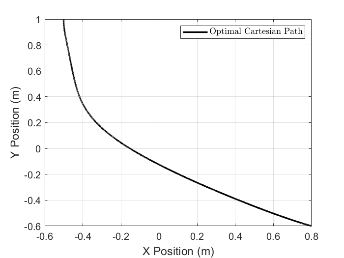
Figure 1: Cartesian trajectory in the $XY$ plane.

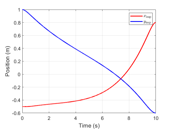
Figure 2: Positions in the Cartesian space: $x_{\mathrm{imp}}$ and $y_{\mathrm{imp}}$.

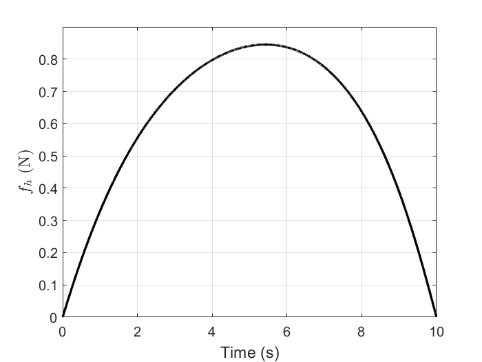
Figure 3: Interaction force $f_{h}$ during human-robot collaboration.

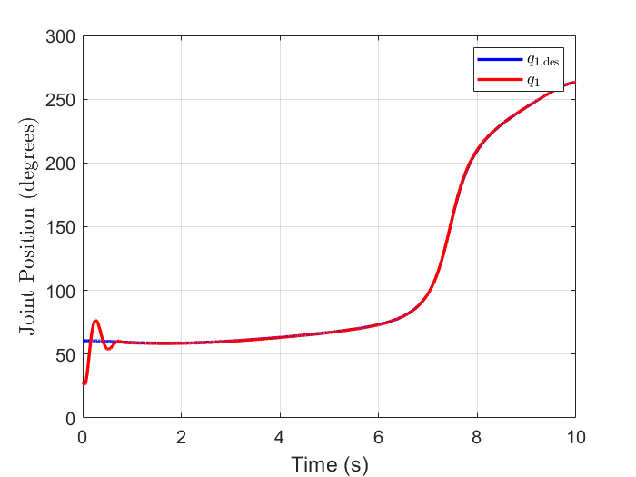
Figure 4: Desired and actual trajectories for the first joint.

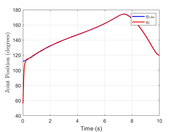
Figure 5: Desired and actual trajectories for the second joint.

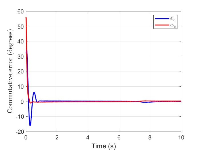
Figure 6: Trajectories of the commutative tracking errors $e_{c_{1}}$ and $e_{c_{2}}$.

VI Conclusion

This paper presented an integrated framework for human-robot collaboration, where the task-specific system dynamics were modeled by combining human impedance and robot interaction behavior. By applying the iDRE, we optimized the trajectory and control inputs without the need for predefined trajectories, enabling time-varying adaptation. The proposed neuro-adaptive PID control method ensured stable and robust tracking performance by dynamically adjusting the PID gains using a neural network. The numerical simulations demonstrated the approach’s adaptability and effectiveness, confirming its potential for real-time applications. Future work will focus on experimental validation in practical settings.

References

- [1] F. L. Lewis, D. Vrabie, and V. Syrmos, Optimal Control, John Wiley & Sons, 2012.
- [2] T. H. Lee and C. J. Harris, Adaptive Neural Network Control of Robotic Manipulators, World Scientific, 1998.
- [3] F. L. Lewis, D. M. Dawson, and C. T. Abdallah, Robot Manipulator Control: Theory and Practice, CRC Press, 2003.
- [4] J. J. E. Slotine and W. Li, Applied Nonlinear Control, Prentice Hall, 1991.
- [5] H. R. Nohooji, I. Howard, and L. Cui, “Optimal robot-environment interaction using inverse differential Riccati equation,” Asian Journal of Control, vol. 22, no. 4, pp. 1401–1410, 2020.
- [6] M. H. Korayem and H. R. Nohooji, “Trajectory optimization of flexible mobile manipulators using open-loop optimal control method,” in Proc. 1st Int. Conf. Intelligent Robotics and Applications (ICIRA), Wuhan, China, Oct. 2008, pp. 54–63.
- [7] H. R. Nohooji, “Constrained neural adaptive PID control for robot manipulators,” Journal of the Franklin Institute, vol. 357, no. 7, pp. 3907–3923, 2020.
- [8] H. R. Nohooji, I. Howard, and L. Cui, “Neural impedance adaptation for assistive human-robot interaction,” Neurocomputing, vol. 290, pp. 50–59, 2018.
- [9] Q. Chen, Y. Wang, and Y. Song, “Tracking control of self-restructuring systems: A low-complexity neuroadaptive PID approach with guaranteed performance,” IEEE Transactions on Cybernetics, 2021.
- [10] Y. Li and S. S. Ge, “Human-robot collaboration based on motion intention estimation,” IEEE/ASME Transactions on Mechatronics, vol. 19, no. 3, pp. 1007–1014, 2013.
- [11] N. Hogan, “Impedance control: An approach to manipulation: Part II—Implementation,” 1985.
- [12] H. Modares, I. Ranatunga, F. L. Lewis, and D. O. Popa, “Optimized assistive human-robot interaction using reinforcement learning,” IEEE Transactions on Cybernetics, vol. 46, no. 3, pp. 655–667, 2015.
- [13] S. S. Ge, Y. Li, and C. Wang, “Impedance adaptation for optimal robot-environment interaction,” International Journal of Control, vol. 87, no. 2, pp. 249–263, 2014.
- [14] Y. Li, K. P. Tee, R. Yan, W. L. Chan, and Y. Wu, “A framework of human-robot coordination based on game theory and policy iteration,” IEEE Transactions on Robotics, vol. 32, no. 6, pp. 1408–1418, 2016.
- [15] E. Spyrakos-Papastavridis and J. S. Dai, “Minimally model-based trajectory tracking and variable impedance control of flexible-joint robots,” IEEE Transactions on Industrial Electronics, vol. 68, no. 7, pp. 6031–6041, 2020.
- [16] X. Liu, S. S. Ge, F. Zhao, and X. Mei, “Optimized impedance adaptation of robot manipulator interacting with unknown environment,” IEEE Transactions on Control Systems Technology, vol. 29, no. 1, pp. 411–419, 2020.
- [17] S. Yousefizadeh, J. D. D. Flores Mendez, and T. Bak, “Trajectory adaptation for an impedance controlled cooperative robot according to an operator’s force,” Automation in Construction, vol. 103, pp. 213–220, 2019.