Quantum dissipative effects for a real scalar field coupled to a time-dependent Dirichlet surface in $d+1$ dimensions

Abstract

We study the Dynamical Casimir Effect (DCE) for a real scalar field $\varphi$ in $d+1$ dimensions, in the presence of a mirror that imposes Dirichlet boundary conditions and undergoes time-dependent motion or deformation. Using a perturbative approach, we expand in powers of the deviation of the mirror’s surface $\Sigma$ from a hyperplane, up to fourth order. General expressions for the probability of pair creation induced by motion are derived, and we analyze the impact of space-time dimensionality as well as of the non-linear effects introduced by the fourth-order terms.

1 Introduction

Quantum vacuum fluctuations, in the presence of non trivial boundary conditions, may induce macroscopic manifestations such as the Casimir and related effects [1, 2]. In the Dynamical Casimir Effect (DCE), particles are created out of the quantum vacuum, due to the presence of time-dependent boundary conditions. The latter may adopt different guises, the most prominent among them being a time-dependence in the geometry of the boundaries, which otherwise keep the nature of the condition they impose unaltered. Within this context, the creation of particles in an oscillating one-dimensional cavity containing a moving mirror is a phenomenon that has been received extensive attention, since the pioneering works by Moore [3], and subsequent results by Davies and Fulling [4].

More recent studies have focused on various aspects of the Dynamical Casimir Effect (DCE), highlighting their relevance to diverse physical phenomena [5]. In a perhaps less direct way, the DCE may shed light into the information loss problem and even entanglement entropy [6]. Also, the study of physical observables in moving mirror models [7] sheds light on the physics of evaporating black holes. Note that moving mirrors are an example of entanglement harvesting from the vacuum [8], and that studies have explored their radiation from the point of view of the Equivalence Principle [9]. Finally, in an apparently rather different context, Dirichlet boundary conditions for a quantum field in higher dimensions appear naturally in the subject of D-branes [10, 11].

In this paper, we deal with a massless real scalar field, in $d+1$ dimensions, under the influence of Dirichlet boundary conditions on a space and time dependent surface. The goal is to derive expressions for the imaginary part of the real-time effective action resulting from the integration of the scalar field, which is a functional of the surface. We recall the fact that the imaginary part determines the probability of vacuum decay; indeed, denoting by ${\mathcal{P}}$ that probability, it may be written as ${\mathcal{P}}=2\,{\rm Im}\Gamma$, where $\Gamma$ denotes the effective action. In our case, that probability corresponds to processes whereby the vacuum decays to states containing a certain number of real quanta of the scalar field.

This paper is organized as follows: In Sect. 2, we define the system to be studied in the remainder of the paper and its effective action. Then, in Sect. 3 we focus on the evaluation of the same object in perturbation theory, discarding whenever possible, pieces of the effective action which cannot contribute to its imaginary part. We present results for both the second and the fourth orders in the expansion. Finally, in Sect. 4 we present our conclusions.

2 The system and its effective action

The system that we study here, consists of a massless real scalar field $\varphi(x)$ in $d+1$ dimensions, subjected to Dirichlet boundary conditions on a space-time surface $\Sigma$, but otherwise being described by a free action ${\mathcal{S}}_{0}(\varphi)$:

$${\mathcal{S}}_{0}(\varphi)\,=\,\frac{1}{2}\int d^{d+1}x\,\partial_{\mu}\varphi(x)\partial^{\mu}\varphi(x)\;.$$ (1)

In order to simplify the perturbative calculations, we adopt imaginary-time conventions , such that the metric becomes Euclidean, i.e., $[g_{\mu\nu}]=[{\mathbb{I}}_{\mu\nu}]$, where ${\mathbb{I}}$ is the $(d+1)\times(d+1)$ identity matrix. Space-time indices are, in our conventions, represented by letters from the middle of the Greek alphabet ($\mu,\nu,\ldots$) and run over the values $0,1,\ldots,d$ ($d$ is the number of spatial dimensions). Space-time coordinates are denoted by $x^{\mu}=x_{\mu}$, $x^{0}$ being the imaginary time. Einstein convention of summation over repeated indices in monomial expressions is also assumed. We adopt natural units, such that: $\hbar\equiv 1$ and $c\equiv 1$.

Note that, had the field been free, i.e., devoid of any non trivial boundaries, the effective action would have coincided with ${\mathcal{S}}_{0}$. We want, however, to include the effects of a space-time surface, $\Sigma$, where the field is constrained to vanish. This will produce, when taking into account the scalar field fluctuations, a quantum, one-loop contribution to the effective action, depending just on the surface. We denote this term as $\Gamma(\Sigma)$, and we may write it in terms of a functional integral:

$$e^{-\Gamma(\Sigma)}\;=\;\frac{1}{\mathcal{N}}\;\int{\mathcal{D}}\varphi\,\delta_{\Sigma}(\varphi)\,e^{-{\mathcal{S}}_{0}(\varphi)}\;\;,\;\;\;{\mathcal{N}}\,=\,\int{\mathcal{D}}\varphi\,e^{-{\mathcal{S}}_{0}(\varphi)}\;.$$ (2)

Here, $\delta_{\Sigma}(\varphi)$ represents a Dirac $\delta$ functional, imposing Dirichlet conditions for $\varphi$ on the surface. An important remark is in order here: we shall be only interested in the imaginary part of $\Gamma(\Sigma)$, after rotating this object back to real time. In particular, this implies that we may safely discard all the local, divergent counterterms that will arise.

In what follows, we make an assumption about the surface, namely, that it may be described, at least with a proper choice of coordinate system, by a single Monge patch. More concretely, letting $x_{\shortparallel}\equiv(x^{\alpha})_{\alpha=0}^{d-1}$ denote the first $d$ space-time coordinates, the assumption is that $\Sigma$ can be parametrized as follows:

$$\Sigma\big{)}\;x_{\shortparallel}\;\to\;y\equiv\big{(}x_{\shortparallel},\psi(x_{\shortparallel})\big{)}\;\;,$$

$${\rm or:}\;y^{\mu}\,=\,\delta^{\mu}_{\alpha}x^{\alpha}\,+\,\delta^{\mu}_{d}\,\psi(x_{\shortparallel})\;,$$ (3)

namely, the surface can be described by specifying its height $\psi(x_{\shortparallel})$ at each point $x_{\shortparallel}$ on the $x^{d}=0$ hyperplane.

A convenient way to proceed with the evaluation of $\Gamma(\Sigma)$ is by first representing the functional $\delta$ function by a (functional) Fourier transform. Indeed, introducing an auxiliary field $\lambda(x_{\shortparallel})$, we may write:

$$\delta_{\Sigma}(\varphi)\;=\;\int{\mathcal{D}}\lambda\,e^{i\int d^{d}x_{\shortparallel}\sqrt{g(x_{\shortparallel})}\,\lambda(x_{\shortparallel})\,\varphi(x_{\shortparallel},\psi(x_{\shortparallel}))}\;,$$ (4)

where $g(x_{\shortparallel})$ denotes the determinant of $g_{\alpha\beta}(x_{\shortparallel})$, the induced metric on $\Sigma$:

$$g_{\alpha\beta}(x_{\shortparallel})\,=\,\delta_{\alpha\beta}+\partial_{\alpha}\psi(x_{\shortparallel})\,\partial_{\beta}\psi(x_{\shortparallel})\;\;,\;\;\;g(x_{\shortparallel})\,=\,1+\partial_{\alpha}\psi(x_{\shortparallel})\,\partial_{\alpha}\psi(x_{\shortparallel})\;.$$ (5)

Having in mind, in what follows, this kind of surface and parametrization for $\Sigma$, we use the self-explanatory notation $\Gamma(\psi)$ for the effective action. We see that:

$$e^{-\Gamma(\psi)}\,=\,\frac{1}{\mathcal{N}}\,\int\mathcal{D}\varphi\mathcal{D}\lambda\;e^{-S_{0}(\varphi)+i\int_{x_{\shortparallel}}\lambda(x_{\shortparallel})\sqrt{g(x_{\shortparallel})}\varphi(x_{\shortparallel},\psi(x_{\shortparallel}))}$$ (6)

where we have used a self-explanatory shorthand notation (that we shall use in the remainder of the paper) for the integrals:

$$\int d^{d+1}x\ldots\equiv\int_{x}\ldots\;\;,\int d^{d}x_{\shortparallel}\ldots\equiv\int_{x_{\shortparallel}}\ldots\;\;,\;\;\ldots$$ (7)

As a first step towards the evaluation of $\Gamma(\psi)$, we see that we can get rid of the $\sqrt{g(x_{\shortparallel})}$ factor in the integral, by a redefinition of the $\lambda$ field integration measure; namely, $\lambda(x_{\shortparallel})\rightarrow\lambda(x_{\shortparallel})[g(x_{\shortparallel})]^{-1/2}$, which yields:

$$e^{-\Gamma(\psi)}\,=\,\frac{{\mathcal{J}}_{g}}{\mathcal{N}}\,\int\mathcal{D}\varphi\mathcal{D}\lambda\;e^{-S_{0}(\varphi)+i\int_{x}J_{\Sigma}(x)\varphi(x)}$$ (8)

where ${\mathcal{J}}_{g}$ denotes the Jacobian:

$${\mathcal{J}}_{g}\;=\;\det[\delta^{d}(x_{\shortparallel}-x^{\prime}_{\shortparallel})g^{-1/2}(x_{\shortparallel})]$$ (9)

and:

$$J_{\Sigma}(x)\,\equiv\,\lambda(x_{\shortparallel})\,\delta\left(x_{d}-\psi(x_{\shortparallel})\right)\;.$$ (10)

Thus, by performing the functional integration of $\varphi$, we obtain for $\Gamma(\psi)$:

$$e^{-\Gamma(\psi)} =\;\det[\delta^{d}(x_{\shortparallel}-x^{\prime}_{\shortparallel})g^{-1/2}(x_{\shortparallel})]$$

$$\times\int\mathcal{D}\lambda\;\exp\Big{[}-\frac{1}{2}\int_{x_{\shortparallel},x^{\prime}_{\shortparallel}}\;\lambda(x_{\shortparallel})\,\Delta(x_{\shortparallel},x^{\prime}_{\shortparallel})\,\lambda(x^{\prime}_{\shortparallel})\Big{]}\;,$$ (11)

with

$$\Delta(x_{\shortparallel},x^{\prime}_{\shortparallel})\;=\;\langle x_{\shortparallel},\psi(x_{\shortparallel})|(-\partial^{2})^{-1}|x^{\prime}_{\shortparallel},\psi(x^{\prime}_{\shortparallel})\rangle\;,$$ (12)

where

$$\langle x_{\shortparallel},x_{d}|(-\partial^{2})^{-1}|x^{\prime}_{\shortparallel},x^{\prime}_{d}\rangle\;=\;\langle x|(-\partial^{2})^{-1}|x^{\prime}\rangle\;=\;\int\frac{d^{d+1}k}{(2\pi)^{d+1}}\frac{e^{ik\cdot(x-x^{\prime})}}{k^{2}}\;,$$ (13)

denotes the free scalar field propagator. By integration out $k_{d}$, we may write for $\Delta$ a more explicit expression

$$\Delta(x_{\shortparallel},x^{\prime}_{\shortparallel})\;=\;\int\frac{d^{d}k_{\shortparallel}}{(2\pi)^{d}}\,e^{ik_{\shortparallel}\cdot(x_{\shortparallel}-x^{\prime}_{\shortparallel})}\,\frac{e^{-|k_{\shortparallel}||\psi(x_{\shortparallel})-\psi(x^{\prime}_{\shortparallel})|}}{2|k_{\shortparallel}|}\;.$$ (14)

The integral over $\lambda$ is a Gaussian. Performing it, produces the result that allows us to write for $\Gamma(\psi)$ the following:

$$e^{-\Gamma(\psi)}\;=\;\Big{\{}\det\big{[}g(x_{\shortparallel})\,\delta^{d}(x_{\shortparallel}-x^{\prime}_{\shortparallel})\big{]}\times\det\big{[}\Delta(x_{\shortparallel},x^{\prime}_{\shortparallel})\big{]}\Big{\}}^{-1/2}\;.$$ (15)

Therefore,

$$\Gamma(\psi)\;=\;\Gamma_{g}(\psi)\,+\,\Gamma_{\Delta}(\psi)$$ (16)

where $\Gamma_{g}(\psi)=\frac{1}{2}{\rm Tr}\big{\{}\log\big{[}g(x_{\shortparallel})\delta^{d}(x_{\shortparallel}-x^{\prime}_{\shortparallel})\big{]}\big{\}}$ and:

$$\Gamma_{\Delta}(\psi)\;=\;\frac{1}{2}{\rm Tr}\big{\{}\log\big{[}\Delta(x_{\shortparallel},x^{\prime}_{\shortparallel})\big{]}\Big{\}}\;.$$ (17)

Before proceeding to the perturbative evaluation, we note that the first term, $\Gamma_{g}(\psi)$, cannot contribute to the imaginary part. Indeed, we first note that it requires the introduction of an $UV$ cutoff $\Lambda$, since it involves a Dirac $\delta$ function evaluated at the coincident points $x_{\shortparallel}$, $x^{\prime}_{\shortparallel}$:

$$\Gamma_{g}(\psi)\,=\,\frac{1}{2}\Lambda^{d}\int_{x_{\shortparallel}}\log\big{[}g(x_{\shortparallel})\big{]}\;.$$ (18)

In real time, then one has:

$$\Gamma_{g}(\psi)\,=\,\frac{1}{2}\Lambda^{d}\int_{x_{\shortparallel}}\log\big{[}1-(\partial_{0}\psi)^{2}+(\nabla_{\shortparallel}\psi)^{2}\big{]}\;,$$ (19)

which can only develop an imaginary part for superluminal excitations of the surface. Therefore, in what follows we concentrate on the remaining term, $\Gamma_{\Delta}$.

3 Expansion in powers of $\psi$

With the aim to evaluate $\Gamma_{\Delta}$, we expand it in powers of $\psi$. To that end, we first expand $\Delta$

$$\Delta\;=\;\Delta^{(0)}\,+\,\Delta^{(1)}\,+\,\ldots$$ (20)

where the index denotes order in $\psi$. We find:

$$\Delta^{(l)}(x_{\shortparallel},x^{\prime}_{\shortparallel}) =\;\int_{\not k_{\shortparallel}}\,\frac{e^{ik_{\shortparallel}(x_{\shortparallel}-x^{\prime}_{\shortparallel})}}{2\big{|}k_{\shortparallel}\big{|}}\;\frac{(-1)^{l}}{l!}\big{|}k_{\shortparallel}\big{|}^{l}\big{|}\psi(x_{\shortparallel})-\psi(x^{\prime}_{\shortparallel})\big{|}^{l}\;,$$ (21)

where we introduced the shorthand notation

$$\int_{\not\!k_{\shortparallel}}\ldots\;\equiv\;\int\frac{d^{d}k}{(2\pi)^{d}}\ldots$$ (22)

We note that $\Delta^{(k)}$ vanishes for odd $k$. To prove that, it is convenient to undo the integral over $k_{d}$, which lead to (14). Then one realizes that

$$\Delta^{(k)}(x_{\shortparallel},x^{\prime}_{\shortparallel}) =\;\frac{i^{k}}{k!}\,\int\frac{d^{d}p_{\shortparallel}}{(2\pi)^{d}}\,e^{ip_{\shortparallel}\cdot(x_{\shortparallel}-x^{\prime}_{\shortparallel})}\int_{-\infty}^{+\infty}\frac{dp_{d}}{2\pi}\frac{p_{d}^{k}}{p_{\shortparallel}^{2}+p_{d}^{2}}\big{(}\psi(x_{\shortparallel})-\psi(x^{\prime}_{\shortparallel})\big{)}^{k}$$

$$=\,0\;\;,\;\;{\rm for}\,{\rm any}\,{\rm odd}\,k\;.$$ (23)

Hence the original expression for $\Delta$ may in fact be represented equivalently as follows:

$$\Delta(x_{\shortparallel},x^{\prime}_{\shortparallel})\;=\;\int_{\not p_{\shortparallel}}\,e^{ip_{\shortparallel}\cdot(x_{\shortparallel}-x^{\prime}_{\shortparallel})}\frac{\cosh\big{[}|p_{\shortparallel}|(\psi(x_{\shortparallel})-\psi(x^{\prime}_{\shortparallel}))\big{]}}{2|p_{\shortparallel}|}\;.$$ (24)

Using the expansion of the $\cosh$,

$$\Gamma_{\Delta}(\psi)\;=\;\frac{1}{2}{\rm Tr}\Big{[}\log\big{(}\Delta^{(0)}\big{)}\Big{]}+\frac{1}{2}{\rm Tr}\Big{[}\log\big{(}1+\sum\limits_{k=1}A^{(2k)}\big{)}\Big{]}$$ (25)

where $A^{(2k)}$ stands for

$$A^{(2k)}(x_{\shortparallel},x^{\prime}_{\shortparallel})\;=\;\int_{y_{\shortparallel}}\;\big{[}\Delta^{(0)}\big{]}^{-1}(x_{\shortparallel},y_{\shortparallel})\;\Delta^{(2k)}(y_{\shortparallel},x^{\prime}_{\shortparallel})\;.$$ (26)

We shall discard the first, zeroth order term in the expansion for $\Gamma_{\Delta}$, since it is a constant independent of $\psi$, and it represents the (divergent) effective action corresponding to the infinite plane $x_{d}=0$. In the context of this expansion, it is the same for any surface. Thus, in what follows, $\Gamma_{\Delta}(\psi)\equiv\frac{1}{2}{\rm Tr}\Big{[}\log\big{(}1+\sum\limits_{k=1}A^{(2k)}\big{)}\Big{]}$, which upon expansion of the logarithm yields,

$$\log\left(1+\sum_{k=1}^{\infty}A^{(2k)}\right)\,=\,\sum_{n=1}^{\infty}\frac{(-1)^{n-1}}{n}\big{[}\sum_{k=1}^{\infty}A^{(2k)}\big{]}^{n}\;,$$ (27)

leading to

$$\Gamma_{\Delta}(\psi)\;=\;\frac{1}{2}\,\sum_{k=1}^{\infty}{\rm Tr}\big{[}A^{(2k)}\big{]}\,-\,\frac{1}{4}\sum_{k=2}^{\infty}\sum_{l=1}^{k-1}{\rm Tr}\big{[}A^{(2k-2l)}\,A^{(2l)}\big{]}$$

$$+\;\frac{1}{6}\,\sum_{k=3}^{\infty}\sum_{l=2}^{k-1}\sum_{m=1}^{l-1}{\rm Tr}\big{[}A^{(2k-2l)}\,A^{(2l-2m)}\,A^{(2m)}\big{]}\;+\;\dots$$ (28)

Regrouping terms,

$$\Gamma_{\Delta}(\psi)\;=\;\Gamma_{\Delta}^{(2)}(\psi)\,+\,\Gamma_{\Delta}^{(4)}(\psi)\,+\,\Gamma_{\Delta}^{(6)}(\psi)\,+\,\ldots$$ (29)

where the explicit form of the first few terms is:

$$\Gamma_{\Delta}^{(2)}(\psi) =\;\frac{1}{2}{\rm Tr}\big{[}A^{(2)}\big{]}\;,$$

$$\Gamma_{\Delta}^{(4)}(\psi) =\;\frac{1}{2}{\rm Tr}\big{[}A^{(4)}\big{]}\,-\,\frac{1}{4}{\rm Tr}\big{[}A^{(2)}A^{(2)}\big{]}$$

$$\Gamma_{\Delta}^{(6)}(\psi) =\;\frac{1}{2}{\rm Tr}\big{[}A^{(6)}\big{]}\,-\,\frac{1}{2}{\rm Tr}\big{[}A^{(4)}A^{(2)}\big{]}\,+\,\frac{1}{6}{\rm Tr}\big{[}A^{(2)}A^{(2)}A^{(2)}\big{]}$$

$$\ldots$$ (30)

Let us now evaluate the first two terms, namely, the ones of order 2 and 4 in $\psi$.

3.1 $\Gamma_{\Delta}^{(2)}$

Introducing the explicit form of $A^{(2)}$, we see that:

$$\Gamma_{\Delta}^{(2)}\;=\;\frac{1}{2}\int_{\not k_{\shortparallel}}\,\big{[}F(0)-F(k_{\shortparallel})\big{]}\,\big{|}\widetilde{\psi}(k_{\shortparallel})\big{|}^{2}\,$$ (31)

where the tilde denotes Fourier transformation ($k_{\shortparallel}$ is a $d$ component momentum). We now evaluate the integral over $p_{\shortparallel}$, rendering $F$ in a form that emphasizes the fact that it is, indeed, a loop integral, albeit with propagators having non-standard exponents (see Fig. 1 ).

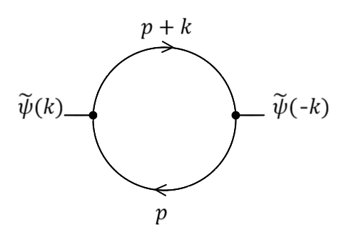
Figure 1: Diagramatic representation of the second order contribution $\Gamma^{(2)}_{\Delta}$.

Namely,

$$F(k_{\shortparallel})\,=\,\int_{\not p_{\shortparallel}}\frac{1}{(p_{\shortparallel}^{2})^{-\frac{1}{2}}[(p_{\shortparallel}+k_{\shortparallel})^{2}]^{-\frac{1}{2}}}\;.$$ (32)

In Fig. 1 a Feynman diagram depicts this contribution. An internal line with momentum $p$ represents $|p_{\shortparallel}|$. The argument of $\widetilde{\psi}$ is positive for ingoing momenta.

The loop integral in (32) is superficially divergent. The (required) zero-momentum subtraction is insufficient to render it finite, but it is possible, however, to apply a procedure devised in a previous reference [12] , involving an analytic regularization. This involves a continuation of the exponents in the would-be propagators, as well as of the number of dimensions. After evaluating the momentum integral, the continuation back to the physical values provides results which allow us to obtain the required result for the imaginary parts.

We proceed then to introduce a Feynman parameter $\alpha$, to generate an expression which generalizes the loop integral we actually need:

$$F_{\lambda_{1},\lambda_{2}}(k_{\shortparallel})\;=\;\frac{\Gamma(\lambda_{1}+\lambda_{2})}{\Gamma(\lambda_{1})\Gamma(\lambda_{2})}\,\int_{0}^{1}d\alpha\;\int_{\not p_{\shortparallel}}\frac{\alpha^{\lambda_{1}-1}(1-\alpha)^{\lambda_{2}-1}}{[\alpha\leavevmode\nobreak\ p_{\shortparallel}^{2}+(1-\alpha)(p_{\shortparallel}+k_{\shortparallel})^{2}]^{\lambda_{1}+\lambda_{2}}}$$ (33)

so that $F=F_{\lambda_{1},\lambda_{2}}\big{|}_{\lambda_{1},\lambda_{2}\to-\frac{1}{2}}$ .

Integrating out the loop momentum,

$$F_{\lambda_{1},\lambda_{2}}(k_{\shortparallel})\,=\,\frac{\Gamma(\lambda_{1}+\lambda_{2}-d/2)}{(4\pi)^{\frac{d}{2}}\Gamma(\lambda_{1})\Gamma(\lambda_{2})}\,\int_{0}^{1}d\alpha\;\alpha^{\frac{d}{2}-\lambda_{2}-1}(1-\alpha)^{\frac{d}{2}-\lambda_{1}-1}\,(k_{\shortparallel}^{2})^{\frac{d}{2}-\lambda_{1}-\lambda_{2}}$$ (34)

so that, for any $d$:

$$F(k_{\shortparallel}) =\frac{1}{(4\pi)^{\frac{d}{2}}}\,\frac{\Gamma(-1-\frac{d}{2})}{[\Gamma(-\frac{1}{2})]^{2}}\,\int_{0}^{1}d\alpha\;\big{[}\alpha(1-\alpha)\big{]}^{\frac{d-1}{2}}\;(k_{\shortparallel}^{2})^{\frac{d+2}{2}}\;,$$ (35)

or, after integrating $\alpha$,

$$F(k_{\shortparallel})\,=\,\frac{1}{(4\pi)^{\frac{d}{2}}}\,\frac{\Gamma(-1-\frac{d}{2})[\Gamma(\frac{d+1}{2})]^{2}}{[\Gamma(-\frac{1}{2})]^{2}\Gamma(d+1)}\,(k_{\shortparallel}^{2})^{\frac{d+2}{2}}\;,$$ (36)

which is a general expression for the kernel of the second order contribution, in principle valid for any $d$, which we recall is the number of spatial dimensions. Some remarks are in order here before obtaining more explicit expressions in particular cases. Firstly, we note that no subtraction at zero momentum is necessary, as the dimensional regularization procedure has already gotten rid of the divergences, subtracting the potentially divergent terms.

To proceed, we note that it is important to distinguish between odd and even values of $d$.

3.1.1 Odd number of spatial dimensions $d=2q+1$ ($q=0,1,\ldots)$

In this case, there is no divergence when taking the limit $d\to(2q+1)$. We find:

$$F(k_{\shortparallel})\,=\,\frac{(-1)^{q}}{(2\pi)^{q+1}}\,\frac{(q!)^{2}}{(2q+1)!(2q+3)!!}\;(k_{\shortparallel}^{2})^{q+\frac{3}{2}}\;.$$ (37)

Therefore,

$$\Gamma^{(2)}_{\Delta}\;=\;\frac{(-1)^{q+1}(q!)^{2}}{2(2\pi)^{q+1}(2q+1)!(2q+3)!!}\;\int_{\not k_{\shortparallel}}|\widetilde{\psi}(k_{\shortparallel})|^{2}\,(k_{\shortparallel}^{2})^{q+1+\frac{1}{2}}\;.$$ (38)

Let us obtain here the real-time version of this contribution, obtained by continuation of the time component of the momentum. We note that the Euclidean $k_{0}$ should be replaced by $-i$ times its real time counterpart, and that $(-)$ times the Euclidean effective action becomes $i$ times its real time version. Denoting by $\Gamma^{(2)}$ the real time effective action corresponding to $\Gamma^{(2)}_{\Delta}$, we get:

$$\Gamma^{(2)}\;=\;\frac{(-1)^{q+1}(q!)^{2}}{2(2\pi)^{q+1}(2q+1)!(2q+3)!!}\;\int_{\not k_{\shortparallel}}\,[{\mathbf{k}}_{\shortparallel}^{2}-(k^{0})^{2}]^{q+1+\frac{1}{2}}\;|\widetilde{\psi}(k^{0},{\mathbf{k}_{\shortparallel}})|^{2}\;,$$ (39)

where, in a natural notation, we have set $k_{\shortparallel}=(k^{0},{\mathbf{k}_{\shortparallel}})$.

We then see that the threshold condition for the appearance of an imaginary part in $\Gamma^{(2)}$ is that the Fourier transform of $\psi$ has components with $|k^{0}|>|{\mathbf{k}}_{\shortparallel}|$. Its explicit form is:

$${\rm Im}\big{[}\Gamma^{(2)}\big{]}\;=\;\frac{1}{2}\;\eta_{2q+1}\,\int_{\not k_{\shortparallel}}\theta(|k^{0}|-|{\mathbf{k}}_{\shortparallel}|)\,\,[(k^{0})^{2}-{\mathbf{k}}_{\shortparallel}^{2}]^{q+1+\frac{1}{2}}\;|\widetilde{\psi}(k^{0},{\mathbf{k}_{\shortparallel}})|^{2}\;,$$ (40)

with $\eta_{2q+1}=\frac{(q!)^{2}}{(2\pi)^{q+1}(2q+1)!(2q+3)!!}$. Note that $\eta_{2q+1}>0$, as it should be, since the probability of vacuum decay must be smaller than $1$.

3.1.2 Even number of spatial dimensions $d=2q$ ($q=1,2,\ldots)$

Since $\Gamma(-1-\frac{d}{2})$ has a pole for even $d$, we set $d=(2q-\epsilon)$, and consider the limit when $\epsilon\to 0$. Note that, to keep the mass dimensions correct, we need to introduce a mass parameter $\mu$. We find, to first order in $\epsilon$:

$$F(k_{\shortparallel})\,=\,\frac{(-1)^{q+1}}{(4\pi)^{q}}\,\frac{\big{[}\Gamma(q+\frac{1}{2})\big{]}^{2}}{(q+1)!(2q)!\big{[}\Gamma(-\frac{1}{2})\big{]}^{2}}\;\left(\frac{2}{\epsilon}-\gamma_{E}\right)(k_{\shortparallel}^{2})^{q+1}\big{[}1-\frac{\epsilon}{2}\log(\frac{k_{\shortparallel}^{2}}{4\pi\mu^{2}})\big{]}\;.$$ (41)

where $\gamma_{E}$ is the Euler-Mascheroni constant.

One of the contributions is divergent when $\epsilon\to 0$, and corresponds to a counterterm which is analytic in $k_{\shortparallel}^{2}$, and thus cannot contribute to the imaginary part, while the term proportional to $\gamma_{E}$ is also analytic in $k_{\shortparallel}^{2}$. This leaves just one contributing term, since it involves a $\log$ function that can have a negative argument,

$$F(k_{\shortparallel})\,=\,\frac{(-1)^{q+2}}{(4\pi)^{q}}\,\frac{\big{[}\Gamma(q+\frac{1}{2})\big{]}^{2}}{(q+1)!(2q)!\big{[}\Gamma(-\frac{1}{2})\big{]}^{2}}\;(k_{\shortparallel}^{2})^{q+1}\log(\frac{k_{\shortparallel}^{2}}{4\pi\mu^{2}})\;+\,\textrm{real terms}.$$ (42)

Therefore,

$${\rm Im}\big{[}\Gamma^{(2)}\big{]}\;=\;\frac{1}{2}\;\eta_{2q}\,\int_{\not k_{\shortparallel}}\theta(|k^{0}|-|{\mathbf{k}}_{\shortparallel}|)\,\,[(k^{0})^{2}-{\mathbf{k}}_{\shortparallel}^{2}]^{q+1}\;|\widetilde{\psi}(k^{0},{\mathbf{k}_{\shortparallel}})|^{2}\;,$$ (43)

where now $\eta_{2q}=\frac{\pi}{(4\pi)^{q}}\,\frac{\big{[}\Gamma(q+\frac{1}{2})\big{]}^{2}}{(q+1)!(2q)!\big{[}\Gamma(-\frac{1}{2})\big{]}^{2}}$.

The successions $\eta_{2q+1}$ and $\eta_{2q}$ behave similarly with growing dimensions, since they are both positive and decrease rapidly as functions of $q$. We plot them in logarithmic scale in figure 2, where we can see their linear behaviour with negative slopes, which indicates an exponential decline in their values.

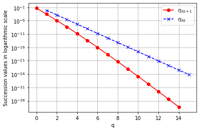
Figure 2: Successions $\eta_{2q+1}$ and $\eta_{2q}$ in logarithmic scale.

3.2 Evaluation of $\Gamma^{(4)}_{\Delta}$

Because of the complexity of the full expression for this term, we shall focus here on its evaluation for a particular, but rather relevant excitation of the surface: a plane wave characterized by a wave vector $k_{\shortparallel}$. As we shall see, the appearance of higher powers of $\tilde{\psi}$, due to the higher powers of $A$ in (3), will translate into higher multiples of the momentum vector $k_{\shortparallel}$ in the decay probability.

For the sake of clarity, we will divide this contribution as $\Gamma_{\Delta}^{(4)}=\Gamma_{\Delta}^{(4,1)}+\Gamma_{\Delta}^{(4,2)}$, where

$$\Gamma_{\Delta}^{(4,1)}=\frac{1}{2}{\rm Tr}\left[A^{(4)}\right].$$ (44)

and

$$\Gamma_{\Delta}^{(4,2)}=-\frac{1}{4}{\rm Tr}\left[A^{(2)}\,A^{(2)}\right]\;.$$ (45)

So we begin with:

$$\Gamma_{\Delta}^{(4,1)} =\frac{1}{48}\int_{x_{\shortparallel}\,x^{\prime}_{\shortparallel}\,\not{k_{\shortparallel}}\,\not{k_{\shortparallel}}^{\prime}}e^{ik_{\shortparallel}(x_{\shortparallel}-x^{\prime}_{\shortparallel})}e^{ik_{\shortparallel}^{\prime}(x_{\shortparallel}^{\prime}-x_{\shortparallel})}\left|k_{\shortparallel}\right|\left|k^{\prime}_{\shortparallel}\right|^{3}\left(\psi(x_{\shortparallel})-\psi(x^{\prime}_{\shortparallel})\right)^{4}$$ (46)

$$=\frac{1}{24}\int_{x_{\shortparallel}\,\not{k_{\shortparallel}}}\,\left|k_{\shortparallel}\right|^{4}\psi(x_{\shortparallel})^{4}+\frac{1}{8}\int\limits_{\not{k_{\shortparallel}}}\tilde{\psi^{2}}(k_{\shortparallel})\tilde{\psi^{2}}(-k_{\shortparallel})\;G(k_{\shortparallel})-\frac{1}{6}\int_{\not{k_{\shortparallel}}}\tilde{\psi^{3}}(k_{\shortparallel})\tilde{\psi}(-k_{\shortparallel})\;G(k_{\shortparallel})$$

$$=\int_{\not{k_{\shortparallel}}}\left[\tilde{\psi^{2}}(k_{\shortparallel})\tilde{\psi^{2}}(-k_{\shortparallel})\left(\frac{G(0_{\shortparallel})}{24}+\frac{G(k_{\shortparallel})}{8}\right)-\frac{1}{6}\tilde{\psi^{3}}(k_{\shortparallel})\tilde{\psi}(-k_{\shortparallel})\;G(k_{\shortparallel})\right],$$

where

$$G(k_{\shortparallel})=\int_{\not{p_{\shortparallel}}}\left|p_{\shortparallel}\right|^{3}\left|p_{\shortparallel}+k_{\shortparallel}\right|=\int_{\not{k}}\frac{1}{(p_{\shortparallel}^{2})^{-\frac{3}{2}}}\frac{1}{((p_{\shortparallel}+k_{\shortparallel})^{2})^{-\frac{1}{2}}}\;.$$ (47)

The different terms in this contribution are illustrated in figure 3. The number of legs of each external line indicates the power of $\psi$, and for internal lines, their number indicates the power of the momentum they carry. Note that the total number of external legs should always match the total number of internal lines.

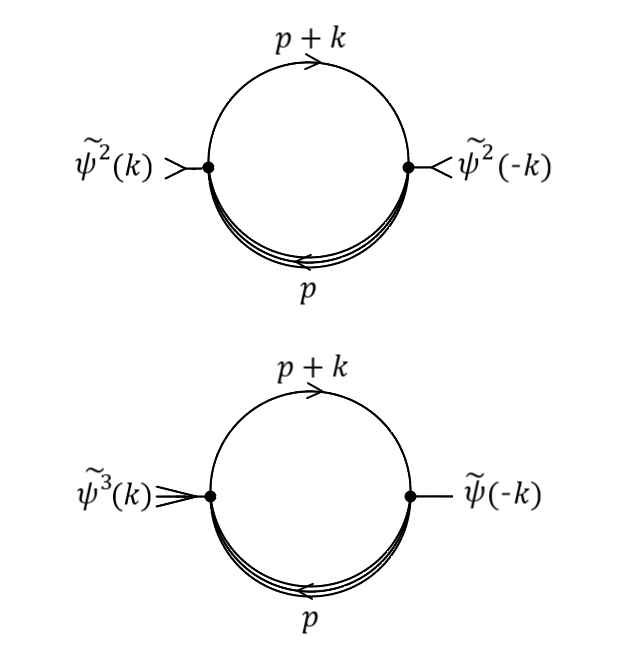
Figure 3: Diagramatic representation of the fourth order contribution $\Gamma_{\Delta}^{(4,1)}$.

Using essentially the same proccedure as in (33), we get:

$$G(k_{\shortparallel}) =\frac{\Gamma(\lambda_{1}+\lambda_{2}-\frac{d}{2})}{\Gamma(\lambda_{1})\Gamma(\lambda_{2})}\int\limits_{0}^{1}d\alpha\;\alpha^{\lambda_{1}-1}(1-\alpha)^{\lambda_{2}-1}\frac{\left(\alpha(1-\alpha)k_{\shortparallel}^{2}\right)^{\frac{d}{2}-(\lambda_{1}+\lambda_{2})}}{(4\pi)^{\frac{d}{2}}}$$ (48)

$$=\frac{\Gamma(\lambda_{1}+\lambda_{2}-\frac{d}{2})}{(4\pi)^{\frac{d}{2}}\Gamma(\lambda_{1})\Gamma(\lambda_{2})}\int\limits_{0}^{1}d\alpha\;\alpha^{\frac{d}{2}-\lambda_{2}-1}(1-\alpha)^{\frac{d}{2}-\lambda_{1}-1}\,(k_{\shortparallel}^{2})^{\frac{d}{2}-\lambda_{1}-\lambda_{2}}$$

$$=\frac{\Gamma(-2-\frac{d}{2})\,\Gamma(\frac{d+3}{2})\Gamma(\frac{d+1}{2})}{(4\pi)^{\frac{d}{2}}\Gamma(-\frac{3}{2})\Gamma(-\frac{1}{2})\Gamma(d+2)}(k_{\shortparallel}^{2})^{\frac{d}{2}+2}\,.$$

Now we move on to the second term of the contribution,

$$\Gamma_{\Delta}^{(4,2)} =-\frac{1}{4}{\rm Tr}\left[A^{(2)}\,A^{(2)}\right]$$ (49)

$$=-\frac{1}{16}\int_{X_{\shortparallel},\not{K_{\shortparallel}}}e^{i\left[k_{\shortparallel}(x_{\shortparallel}-y_{\shortparallel})+k^{\prime}_{\shortparallel}(y_{\shortparallel}-y^{\prime}_{\shortparallel})+q_{\shortparallel}(y^{\prime}_{\shortparallel}-x^{\prime}_{\shortparallel})+q^{\prime}_{\shortparallel}(x^{\prime}_{\shortparallel}-x_{\shortparallel})\right]}$$

$$\times\left|k_{\shortparallel}\right|\left|k^{\prime}_{\shortparallel}\right|\left|q_{\shortparallel}\right|\left|q^{\prime}_{\shortparallel}\right|\left(\psi(y_{\shortparallel})-\psi(y^{\prime}_{\shortparallel})\right)^{2}\left(\psi(x_{\shortparallel})-\psi(x^{\prime}_{\shortparallel})\right)^{2}$$

where $\int_{X_{\shortparallel},\not{K_{\shortparallel}}}$ indicates integration over all space-time and momentum variables respectively. This integral separates into 9 terms, since

$$\left(\psi(x_{\shortparallel})-\psi(x^{\prime}_{\shortparallel})\right)^{2}\left(\psi(y_{\shortparallel})-\psi(y^{\prime}_{\shortparallel})\right)^{2}=$$ (50)

$$=\psi^{2}(x_{\shortparallel})\psi^{2}(y_{\shortparallel})+\psi^{2}(x_{\shortparallel})\psi^{2}(y^{\prime}_{\shortparallel})+\psi^{2}(x^{\prime}_{\shortparallel})\psi^{2}(y_{\shortparallel})+\psi^{2}(x^{\prime}_{\shortparallel})\psi^{2}(y^{\prime}_{\shortparallel})$$

$$-2\left[\psi(x_{\shortparallel})\psi(x^{\prime}_{\shortparallel})\psi^{2}(y_{\shortparallel})+\psi(x_{\shortparallel})\psi(x^{\prime}_{\shortparallel})\psi^{2}(y^{\prime}_{\shortparallel})+\psi(y_{\shortparallel})\psi(y^{\prime}_{\shortparallel})\psi^{2}(x_{\shortparallel})+\psi(y_{\shortparallel})\psi(y^{\prime}_{\shortparallel})\psi^{2}(x^{\prime}_{\shortparallel})\right]$$

$$+4\psi(x_{\shortparallel})\psi(x^{\prime}_{\shortparallel})\psi(y_{\shortparallel})\psi(y^{\prime}_{\shortparallel}).$$

For convenience, we will separate (50) into three different contributions that have different kernels, as we will show below. We write said separation as

$$\Gamma_{\Delta}^{(4,2)}=-\frac{1}{16}\Gamma_{A}+\frac{1}{8}\Gamma_{B}-\frac{1}{4}\Gamma_{C},$$ (51)

being $\Gamma_{A}$ the integral with the four terms in the first line in (50), $\Gamma_{B}$ the one with the second line, and $\Gamma_{C}$ the one with the third line.

We start with

$$\Gamma_{A} =\int_{X_{\shortparallel},\not{K_{\shortparallel}}}e^{i\left[k_{\shortparallel}(x_{\shortparallel}-y_{\shortparallel})+k^{\prime}_{\shortparallel}(y_{\shortparallel}-y^{\prime}_{\shortparallel})+q_{\shortparallel}(y^{\prime}_{\shortparallel}-x^{\prime}_{\shortparallel})+q^{\prime}_{\shortparallel}(x^{\prime}_{\shortparallel}-x_{\shortparallel})\right]}\left|k_{\shortparallel}\right|\left|k^{\prime}_{\shortparallel}\right|\left|q_{\shortparallel}\right|\left|q^{\prime}_{\shortparallel}\right|\times$$ (52)

$$\left[\psi^{2}(x^{\prime}_{\shortparallel})\psi^{2}(y^{\prime}_{\shortparallel})+\psi^{2}(x^{\prime}_{\shortparallel})\psi^{2}(y_{\shortparallel})+\psi^{2}(x_{\shortparallel})\psi^{2}(y^{\prime}_{\shortparallel})+\psi^{2}(x_{\shortparallel})\psi^{2}(y_{\shortparallel})\right]$$

$$=2\int_{\not{K_{\shortparallel}}}(2\pi)^{2d}\delta^{d}(q^{\prime}_{\shortparallel}-k_{\shortparallel})\delta^{d}(k_{\shortparallel}-k^{\prime}_{\shortparallel})\tilde{\psi^{2}}(q_{\shortparallel}-q^{\prime}_{\shortparallel})\tilde{\psi^{2}}(k^{\prime}_{\shortparallel}-q_{\shortparallel})\left|k_{\shortparallel}\right|\left|k^{\prime}_{\shortparallel}\right|\left|q_{\shortparallel}\right|\left|q^{\prime}_{\shortparallel}\right|$$

$$+2\int_{\not{K_{\shortparallel}}}(2\pi)^{2d}\delta^{d}(q^{\prime}_{\shortparallel}-q_{\shortparallel})\delta^{d}(k_{\shortparallel}-k^{\prime}_{\shortparallel})\tilde{\psi^{2}}(q_{\shortparallel}-q^{\prime}_{\shortparallel})\tilde{\psi^{2}}(k^{\prime}_{\shortparallel}-q_{\shortparallel})\left|k_{\shortparallel}\right|\left|k^{\prime}_{\shortparallel}\right|\left|q_{\shortparallel}\right|\left|q^{\prime}_{\shortparallel}\right|$$

$$=2\int_{\not{q_{\shortparallel}}\,\not{q_{\shortparallel}}^{\prime}}\left(|q^{\prime}_{\shortparallel}|^{3}|q_{\shortparallel}|+|q^{\prime}_{\shortparallel}|^{2}|q_{\shortparallel}|^{2}\right)\,\tilde{\psi^{2}}(q_{\shortparallel}-q^{\prime}_{\shortparallel})\tilde{\psi^{2}}(q^{\prime}_{\shortparallel}-q_{\shortparallel})$$

$$=2\int_{\not{k_{\shortparallel}}}\tilde{\psi^{2}}(k_{\shortparallel})\tilde{\psi^{2}}(-k_{\shortparallel})\;G(k_{\shortparallel})+\,\text{real term}\,,$$

with $G(k_{\shortparallel})$ defined by (48). This corresponds to the first diagram in figure 3. We’re not interested in the term with the product $|q^{\prime}_{\shortparallel}|^{2}|q_{\shortparallel}|^{2}$ since it can’t contribute to the imaginary part, so we discard it. Then we procceed with the term

$$\Gamma_{B} =\int_{X_{\shortparallel},\not{K_{\shortparallel}}}e^{i\left[k_{\shortparallel}(x_{\shortparallel}-y_{\shortparallel})+k^{\prime}_{\shortparallel}(y_{\shortparallel}-y^{\prime}_{\shortparallel})+q_{\shortparallel}(y^{\prime}_{\shortparallel}-x^{\prime}_{\shortparallel})+q^{\prime}_{\shortparallel}(x^{\prime}_{\shortparallel}-x_{\shortparallel})\right]}\left|k_{\shortparallel}\right|\left|k^{\prime}_{\shortparallel}\right|\left|q_{\shortparallel}\right|\left|q^{\prime}_{\shortparallel}\right|\times$$ (53)

$$\left[\psi(x_{\shortparallel})\psi(x^{\prime}_{\shortparallel})\psi^{2}(y_{\shortparallel})+\psi(x_{\shortparallel})\psi(x^{\prime}_{\shortparallel})\psi^{2}(y^{\prime}_{\shortparallel})+\psi(y_{\shortparallel})\psi(y^{\prime}_{\shortparallel})\psi^{2}(x_{\shortparallel})+\psi(y_{\shortparallel})\psi(y^{\prime}_{\shortparallel})\psi^{2}(x^{\prime}_{\shortparallel})\right]$$

$$=2\int_{\not{p_{\shortparallel}}\,\not{q_{\shortparallel}}}\left(\tilde{\psi}(-p_{\shortparallel})\tilde{\psi}(-q_{\shortparallel})\tilde{\psi^{2}}(p_{\shortparallel}+q_{\shortparallel})H(p_{\shortparallel},q_{\shortparallel})+\tilde{\psi}(p_{\shortparallel})\tilde{\psi}(q_{\shortparallel})\tilde{\psi^{2}}(-p_{\shortparallel}-q_{\shortparallel})H(-q_{\shortparallel},-p_{\shortparallel})\right),$$

where

$$H(p_{\shortparallel},q_{\shortparallel})=\int_{\not{k_{\shortparallel}}}\left|k_{\shortparallel}\right|^{2}\left|k_{\shortparallel}-p_{\shortparallel}\right|\left|k_{\shortparallel}-p_{\shortparallel}-q_{\shortparallel}\right|=\int\limits_{\not{k_{\shortparallel}}}\frac{k_{\shortparallel}^{2}}{((k_{\shortparallel}-p_{\shortparallel})^{2})^{-\frac{1}{2}}((k_{\shortparallel}-p_{\shortparallel}-q_{\shortparallel})^{2})^{-\frac{1}{2}}}.$$ (54)

This contribution is illustrated in figure 4. We can deal with (54) as in (33) and (48),

$$\int_{\not{k_{\shortparallel}}}\frac{k_{\shortparallel}^{2}}{((k_{\shortparallel}-p_{\shortparallel})^{2})^{-\frac{1}{2}}((k_{\shortparallel}-p_{\shortparallel}-q_{\shortparallel})^{2})^{-\frac{1}{2}}}=$$

$$=\;\frac{\Gamma(\lambda_{1}+\lambda_{2})}{\Gamma(\lambda_{1})\Gamma(\lambda_{2})}\int_{0}^{1}d\alpha\;\alpha^{\lambda_{1}-1}(1-\alpha)^{\lambda_{2}-1}\,\int_{\not{p_{\shortparallel}}}\frac{g_{\mu\nu}\,k_{\shortparallel}^{\mu}k_{\shortparallel}^{\nu}}{(\alpha\leavevmode\nobreak\ p^{2}+(1-\alpha)(p_{\shortparallel}+k_{\shortparallel})^{2})^{\lambda_{1}+\lambda_{2}}}\,,$$ (55)

where we plug in $\lambda_{1}=\lambda_{2}=-\frac{1}{2}$ after integration. Since this equation has components of the loop variable on the numerator, we use the following formulae:

$$\int_{\not{k_{\shortparallel}}}\frac{k_{\shortparallel}^{\mu}k_{\shortparallel}^{\nu}}{\left(k_{\shortparallel}^{2}+2\,Q\,k_{\shortparallel}+C\right)^{a}}=\left(Q^{\mu}Q^{\nu}+g^{\mu\nu}\frac{(C-Q^{2})}{2}\frac{\Gamma(a-\frac{d}{2}-1)}{\Gamma(a-\frac{d}{2})}\right)I_{0}$$ (56)

with

$$I_{0}=\frac{\left(C-Q^{2}\right)^{\frac{d}{2}-a}}{(4\pi)^{\frac{d}{2}}}\frac{\Gamma(a-\frac{d}{2})}{\Gamma(a)}$$ (57)

in Euclidean formalism, where $g^{\mu\nu}$ is just the identity.

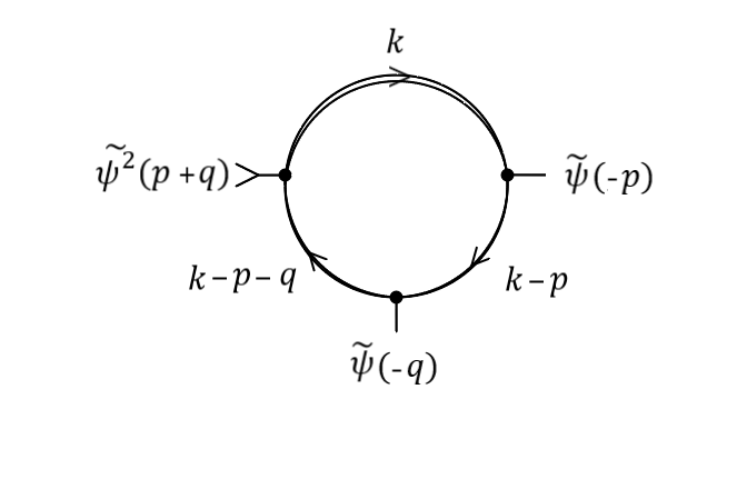
Figure 4: Diagramatic representation of the fourth order contribution $\Gamma_{B}$.

Then

$$H(p_{\shortparallel},q_{\shortparallel})\;=\;\frac{\Gamma(-1-\frac{d}{2})}{\Gamma(-\frac{1}{2})\Gamma(-\frac{1}{2})}\frac{(q_{\shortparallel}^{2})^{\frac{d}{2}+1}}{(4\pi)^{\frac{d}{2}}}$$

$$\times\Big{[}p_{\shortparallel}^{2}\frac{(\Gamma(\frac{d+1}{2}))^{2}}{\Gamma(d+1)}+2p_{\shortparallel}q_{\shortparallel}\frac{\Gamma(\frac{d+1}{2})\Gamma(\frac{d+3}{2})}{\Gamma(d+2)}+q_{\shortparallel}^{2}\frac{\Gamma(\frac{d+1}{2})\Gamma(\frac{d+5}{2})}{\Gamma(d+3)}$$

$$+\;\frac{d}{2}q_{\shortparallel}^{2}\,\frac{(\Gamma(\frac{d+3}{2}))^{2}}{\Gamma(d+3)}\,\frac{\Gamma(-2-\frac{d}{2})}{\Gamma(-1-\frac{d}{2})}\Big{]}\,.$$ (58)

Finally,

$$\Gamma_{C}\;=\;\int_{\not{k_{\shortparallel}}\,\not{p_{\shortparallel}}\,\not{q_{\shortparallel}}}\tilde{\psi}(-k_{\shortparallel})\tilde{\psi}(-p_{\shortparallel})\tilde{\psi}(-q_{\shortparallel})\tilde{\psi}(k_{\shortparallel}+p_{\shortparallel}+q_{\shortparallel})\,K(k_{\shortparallel},p_{\shortparallel},q_{\shortparallel}),$$ (59)

with

$$K(k_{\shortparallel},p_{\shortparallel},q_{\shortparallel})=\int_{\not{\ell}_{\shortparallel}}|\ell_{\shortparallel}||\ell_{\shortparallel}+k_{\shortparallel}||\ell_{\shortparallel}+k_{\shortparallel}+p_{\shortparallel}||\ell_{\shortparallel}+k_{\shortparallel}+p_{\shortparallel}+q_{\shortparallel}|\;.$$ (60)

This integral, with different powers of the propagators, is known as the scalar box integral, illustrated in figure 5. It has been dealt with applying different mass conditions on the internal and external momentum lines, as well as in the on-shell or off-shell conditions for them, for example in [13], [14] and [15]. However, in our case the kernel is defined trough negative and rational powers of the propagators, which gives divergent integrals when using Feynman parametrization in (60). For this reason, we procceed to solve the integral by imposing a specific form for $\psi(x_{\shortparallel})$.

3.3 Wave-like surface

We can obtain a result for (60) if the surface takes the form

$$\psi(x_{\shortparallel})=2A\,{\rm cos}(\omega_{0}\,x_{0}-\bm{\omega}_{\shortparallel}\bm{x}_{\shortparallel}),$$ (61)

defining the vector $\omega_{\shortparallel}=(\omega_{0},\bm{\omega}_{\shortparallel})$ where $\bm{\omega}_{\shortparallel}$ and $\bm{x}_{\shortparallel}$ have their components ranging from $1$ to $d-1$. Then we have

$$\tilde{\psi}(k_{\shortparallel}) =A\,(2\pi)^{d}\left[\delta^{d}(k_{\shortparallel}-\omega_{\shortparallel})+\delta^{d}(k_{\shortparallel}+\omega_{\shortparallel})\right]$$ (62)

$$\tilde{\psi^{2}}(k_{\shortparallel}) =A^{2}(2\pi)^{d}\left[\delta^{d}(k_{\shortparallel}-2\omega_{\shortparallel})+\delta^{d}(k_{\shortparallel}+2\omega_{\shortparallel})+2\delta^{d}(k_{\shortparallel})\right]$$

$$\tilde{\psi^{3}}(k_{\shortparallel}) =A^{3}(2\pi)^{d}\left[\delta^{d}(k_{\shortparallel}-3\omega_{\shortparallel})+\delta^{d}(k_{\shortparallel}+3\omega_{\shortparallel})+3\delta^{d}(k_{\shortparallel}-\omega_{\shortparallel})+3\delta^{d}(k_{\shortparallel}+\omega_{\shortparallel})\right],$$

where we see the tendency that the $n$-th power of the expansion involves a $n$-multiple of the wave vector.

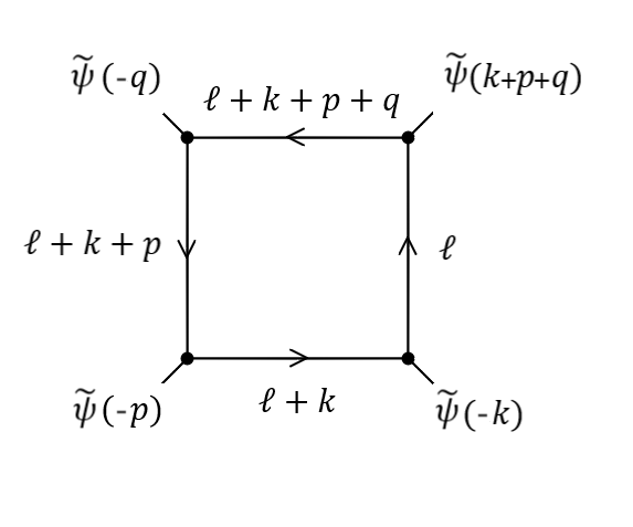
Figure 5: Scalar box integral for the contribution $\Gamma_{C}$.

This leads to

$$\Gamma_{C} =\int_{\not{k_{\shortparallel}}\,\not{p_{\shortparallel}}\,\not{q_{\shortparallel}}}\tilde{\psi}(-k_{\shortparallel})\tilde{\psi}(-p_{\shortparallel})\tilde{\psi}(-q_{\shortparallel})\tilde{\psi}(k_{\shortparallel}+p_{\shortparallel}+q_{\shortparallel})\,K(k_{\shortparallel},p_{\shortparallel},q_{\shortparallel})$$ (63)

$$=A^{4}(2\pi)^{2d}$$

$$\times\int_{\not{k_{\shortparallel}}\,\not{p_{\shortparallel}}\,\not{q_{\shortparallel}}}\left[\delta^{d}(k_{\shortparallel}-\omega_{\shortparallel})+\delta^{d}(k_{\shortparallel}+\omega_{\shortparallel})\right]\left[\delta^{d}(p_{\shortparallel}-\omega_{\shortparallel})+\delta^{d}(p_{\shortparallel}+\omega_{\shortparallel})\right]$$

$$\times\left[\delta^{d}(q_{\shortparallel}-\omega_{\shortparallel})+\delta^{d}(q_{\shortparallel}+\omega_{\shortparallel})\right]\left[\delta^{d}((k_{\shortparallel}+p_{\shortparallel}+q_{\shortparallel})-\omega_{\shortparallel})+\delta^{d}((k_{\shortparallel}+p_{\shortparallel}+q_{\shortparallel})+\omega_{\shortparallel})\right]$$

$$\times\int_{\not{\ell}_{\shortparallel}}|\ell_{\shortparallel}||\ell_{\shortparallel}+k_{\shortparallel}||\ell_{\shortparallel}+k_{\shortparallel}+p_{\shortparallel}||\ell_{\shortparallel}+k_{\shortparallel}+p_{\shortparallel}+q_{\shortparallel}|$$

$$=4A^{4}(2\pi)^{d}\delta^{d}(0)\int\limits_{\not{\ell_{\shortparallel}}}|\ell_{\shortparallel}|^{2}|\ell_{\shortparallel}-\omega_{\shortparallel}||\ell_{\shortparallel}+\omega_{\shortparallel}|+\text{real term,}$$

where the loop integral (60) is now $H(\omega_{\shortparallel},-2\omega_{\shortparallel})$, given by (3.2). Similarly to (52), we discarded a term proportional to $|\ell_{\shortparallel}|^{2}|\ell_{\shortparallel}+\omega_{\shortparallel}|^{2}$ since it doesn’t contribute to the imaginary part.

We note that the factor $(2\pi)^{d}\delta^{d}(0)$ appears, as expected, for a quantity that has been calculated for an infinite region of space-time. This corresponds to the integration hypervolume $T\,V$. This factor will appear on all contributions and can be made sense of by dividing every term by it, getting as a result the respective propabilities per unit time and per spatial volume.

Now using (62) on the previous calculations, we find

$$\Gamma_{\Delta}^{(4,1)} =\frac{\Gamma(-2-\frac{d}{2})\,\Gamma(\frac{d+3}{2})\Gamma(\frac{d+1}{2})}{(4\pi)^{\frac{d}{2}}\Gamma(-\frac{3}{2})\Gamma(-\frac{1}{2})\Gamma(d+2)}\int_{\not{k_{\shortparallel}}}\left(\frac{\tilde{\psi^{2}}(k_{\shortparallel})\tilde{\psi^{2}}(-k_{\shortparallel})}{8}-\frac{\tilde{\psi^{3}}(k_{\shortparallel})\tilde{\psi}(-k_{\shortparallel})}{6}\right)\left(k_{\shortparallel}^{2}\right)^{\frac{d}{2}+2}$$ (64)

$$=\frac{\Gamma(-2-\frac{d}{2})\,\Gamma(\frac{d+3}{2})\Gamma(\frac{d+1}{2})}{(4\pi)^{\frac{d}{2}}\Gamma(-\frac{3}{2})\Gamma(-\frac{1}{2})\Gamma(d+2)}A^{4}\delta^{d}(0)(2\pi)^{d}\left(\frac{1}{4}((2\omega_{\shortparallel})^{2})^{\frac{d}{2}+2}-((\omega_{\shortparallel})^{2})^{\frac{d}{2}+2}\right)$$

$$=\frac{A^{4}\delta^{d}(0)(2\pi)^{d}(\omega_{\shortparallel}^{2})^{{\frac{d}{2}+2}}}{(4\pi)^{\frac{d}{2}}}\,\Gamma(-2-\frac{d}{2})\,(4^{\frac{d+2}{2}}-1)\,a$$

and

$$\Gamma_{\Delta}^{(4,2)} =-\frac{1}{16}\Gamma_{A}+\frac{1}{2}\Gamma_{B}-\frac{1}{4}\Gamma_{C}$$ (65)

$$=\frac{A^{4}(2\pi)^{d}\delta^{d}(0)(\omega_{\shortparallel}^{2})^{\frac{d}{2}+2}}{(4\pi)^{\frac{d}{2}}}$$

$$\times\left[\Gamma(-2-\frac{d}{2})\left(-4^{\frac{d+2}{2}}\,a+d(\frac{3}{2}-4^{\frac{d+3}{2}})\,b\right)+\Gamma(-1-\frac{d}{2})\left(c-4^{\frac{d+2}{2}}e\right)\right]$$

with the definitions:

$$a=\frac{\Gamma(\frac{d+3}{2})\Gamma(\frac{d+1}{2})}{\Gamma(-\frac{3}{2})\Gamma(-\frac{1}{2})(d+1)!}$$ (66)

$$b=\frac{\left(\Gamma(\frac{d+3}{2})\right)^{2}}{\left(\Gamma(-\frac{1}{2})\right)^{2}(d+2)!}$$

$$c=\frac{3\left(\Gamma(\frac{d+1}{2})\right)^{2}}{d\,!\left(\Gamma(-\frac{1}{2})\right)^{2}}+\frac{3\Gamma(\frac{d+1}{2})\Gamma(\frac{d+5}{2})}{\left(\Gamma(-\frac{1}{2})\right)^{2}(d+2)!}-\frac{2\Gamma(\frac{d+1}{2})\Gamma(\frac{d+3}{2})}{\left(\Gamma(-\frac{1}{2})\right)^{2}(d+1)!}$$

$$e=\frac{\left(\Gamma(\frac{d+1}{2})\right)^{2}}{d\,!\left(\Gamma(-\frac{1}{2})\right)^{2}}+\frac{4\Gamma(\frac{d+1}{2})\Gamma(\frac{d+5}{2})}{\left(\Gamma(-\frac{1}{2})\right)^{2}(d+2)!}-\frac{4\Gamma(\frac{d+1}{2})\Gamma(\frac{d+3}{2})}{\left(\Gamma(-\frac{1}{2})\right)^{2}(d+1)!}\;.$$

All these constants can be obtained directly for even and odd dimensions by plugging the value of $d$ without any extra work, since they’re all well defined. Therefore

$$\Gamma_{\Delta}^{(4)} =\Gamma^{(4,1)}_{\Delta}+\Gamma^{(4,2)}_{\Delta}$$ (67)

$$=\frac{A^{4}(2\pi)^{d}\delta^{d}(0)(\omega_{\shortparallel}^{2})^{\frac{d}{2}+2}}{(4\pi)^{\frac{d}{2}}}\,$$

$$\times\left[\Gamma(-2-\frac{d}{2})\left(-\,a+d(\frac{3}{2}-4^{\frac{d+3}{2}})\,b\right)+\Gamma(-1-\frac{d}{2})\left(c-4^{\frac{d+2}{2}}e\right)\right].$$

We see that $\Gamma^{(4)}_{\Delta}$ has a common factor of $(\omega_{\shortparallel}^{2})^{\frac{d}{2}+1}$ where, following the logic we used in sections 3.1.1 and 3.1.2, we identify that for odd $d$ there’s a contribution to the imaginary part that comes from $\sqrt{\bm{\omega}_{\shortparallel}^{2}-\omega_{0}^{2}}\,\theta(|\omega_{0}|-|\bm{\omega}_{\shortparallel}|)$, and for even $d$, using dimensional regularization with $d=(2q-\epsilon)$, there’s a contribution to the imaginary part coming from $\log({\bm{\omega}_{\shortparallel}^{2}-\omega_{0}^{2}})\,\theta(|\omega_{0}|-|\bm{\omega}_{\shortparallel}|)$.

Writing the imaginary part of $\Gamma^{(4)}$, the real time effective action corresponding to $\Gamma^{(4)}_{\Delta}$, as

$${\rm Im}(\Gamma^{(4)})=A^{4}(2\pi)^{d}\delta^{d}(0)\,\zeta_{2q+1}\,\left((\omega^{0})^{2}-\bm{\omega}_{\shortparallel}^{2}\right)^{q+2+\frac{1}{2}}\theta(|\omega^{0}|-|\bm{\omega}_{\shortparallel}|)\,\,\,$$ (68)

for $d=2q+1$ and

$${\rm Im}(\Gamma^{(4)})=A^{4}(2\pi)^{d}\delta^{d}(0)\,\zeta_{2q}\,\left((\omega^{0})^{2}-\bm{\omega}_{\shortparallel}^{2}\right)^{q+2}\theta(|\omega^{0}|-|\bm{\omega}_{\shortparallel}|)$$ (69)

for $d=2q$, we get

$$\zeta_{2q+1}=\frac{(-1)^{q}}{(4\pi)^{q+\frac{1}{2}}}\times$$ (70)

$$\left[\Gamma(-q-\frac{3}{2})(c-4^{q+\frac{3}{2}}e)+\Gamma(-q-\frac{5}{2})\left(-\,a+(2q+1)(\frac{3}{2}-4^{q+2})b\right)\right],$$

and

$$\zeta_{2q} =\frac{\pi}{(4\pi)^{q}}\left[\frac{(c-4^{q+1}e)}{(q+1)!}-\frac{\left(-\,a+2q(\frac{3}{2}-4^{q+\frac{3}{2}})b\right)}{(q+2)!}\right].$$ (71)

The successions $\zeta_{2q+1}$ and $\zeta_{2q}$ are plotted in figure 6. Just like for the second order contribution, these successions are positive and decrease rapidly with growing dimensions, showing a linear behaviour on logarithmic scale.

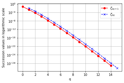
Figure 6: Successions $\zeta_{2q+1}$ and $\zeta_{2q}$ in logarithmic scale.

4 Conclusions

We have evaluated the imaginary part of the effective action, and therefore the corresponding probability of vacuum decay, for a Dirichlet surface in $d+1$ dimensions that can deform and move, in a time-dependent way, under the assumtion of small departures with respect to an average, planar hypersurface. This evaluation has been performed up to the fourth order in the amplitude of the deformation, giving rather explicit expressions for the second order term; while the fourth order one is presented for the case of wave-like deformations of the surface.

In all the terms we have evaluated, there is a common threshold for vacuum decay, namely, that the deformation should have time-like components in Fourier space. Note that, given the (assumed) bounded nature of the deformations, this kind of motion should corresspond, at least locally at each point of the surface, to some sort of oscillatory motion.

We have presented rather general results regarding their dependence on the number of spatial dimensions $d$. The general structure of the decay probability per unit time and per unit volume, does have a dependence on the momenta of the deformation, which may be explained on dimensional grounds. On the other hand, these general results have a dimensionless prefactor, of which we know the dependence with $d$, for which we find a consistent exponential decay when the number of dimensions increases. This means that the process of pair creation by a surface of codimension one seems to be less effective (at least per unit volume) when $d$ becomes larger. The total probability, of course, does have an exponentially growing factor $L^{d}$.

References

[1]
Milton, K. A. (1999).
The Casimir Effect: Physical Manifestations of Zero-Point Energy.
World Scientific.
[2]
Bordag, M., Klimchitskaya, G. L., Mohideen, U., & Mostepanenko, V. M. (2009).
Advances in the Casimir Effect.
Oxford University Press.
[3] G. T. Moore, J. Math. Phys. 11, 2679 (1970).
[4] P. C. W. Davies and S. A. Fulling,
Proc. Roy. Soc. Lond. A 348, 393 (1976); ibidem
Proc. Roy. Soc. Lond. A 356, 237 (1977).
[5] V. V. Dodonov,
Phys. Scripta 82, 038105 (2010); D. A. R. Dalvit, P. A. Maia Neto and F. D. Mazzitelli,
Lect. Notes Phys. 834, 419 (2011);
R. Schutzhold,
arXiv:1110.6064 [quant-ph];
P. D. Nation, J. R. Johansson, M. P. Blencowe and F. Nori,
Rev. Mod. Phys. 84, 1 (2012).
[6] P. Chen and D. h. Yeom,
Phys. Rev. D 96, no. 2, 025016 (2017).
[7]
M. R. R. Good and E. V. Linder, Phys. Rev. D 99, no. 2, 025009
(2019); Phys. Rev. D 97, no. 6, 065006 (2018);
Phys. Rev. D 96, no. 12, 125010 (2017).
[8] W. Cong, E. Tjoa and R. B. Mann,
JHEP 2019, 021 (2020);
Erratum: [JHEP 1907, 051 (2019)].
[9]S. A. Fulling and J. H. Wilson,
Phys. Scripta 94, no. 1, 014004 (2019).
[10]
J. Polchinski,
[arXiv:hep-th/9611050 [hep-th]].
[11]
C. V. Johnson,
doi:10.1017/9781009401371
[12]
C. D. Fosco, F. C. Lombardo and F. D. Mazzitelli.