High Dimensional Space Oddity

Abstract

In his 1996 paper, Talagrand highlighted that the Law of Large Numbers (LLN) for independent random variables can be viewed as a geometric property of multidimensional product spaces. This phenomenon is known as the concentration of measure. To illustrate this profound connection between geometry and probability theory, we consider a seemingly intractable geometric problem in multidimensional Euclidean space and solve it using standard probabilistic tools such as the LLN and the Central Limit Theorem (CLT).

Keywords: Central Limit Theorem, Law of Large Numbers, Multidimensional Euclidian Space, Measure Concentration.

1 Introduction: A Curious Result

“It is through science that we prove, but through intuition that we discover”. Henri Poincaré.

“The only real valuable thing is intuition”. Albert Einstein.

Maybe. Or maybe, intuition is what made Poincaré reject Cantor’s set theory, saying that “There is no actual infinity”, and caused Einstein to oppose the notion of entanglement in quantum physics, suggesting that it implies “spooky action at a distance”.

In probability and statistics, there are many counterexamples [10] which show that one must always be careful trusting one’s intuition. Famously, even the great Paul Erdős could not believe the correct solution to the Monty Hall problem [3]. But maybe all these examples of failed intuition only occur in relatively recent theories? Maybe our geometric intuition is sound? This is definitely not the case in dimension greater than 3. The following example was given in [8] as a cautionary tale, and is the starting point for this paper.

Steele [8] describes an arrangement of $n$-dimensional balls centered around the $2^{n}$ vertices of a cube, $\mathbf{c}_{k}\in\{-1,1\}^{n}$, each with radius 1, as in Figure 1 for $n=2$, and in Figure 2 for $n=3$. The arrangement is bounded by the cube $[-2,2]^{n}$. The question is, if we enclose a sphere centered at the origin so that it is tangent to the spheres in the arrangement, is it in the cube $[-2,2]^{n}$ for all $n\geq 2$?

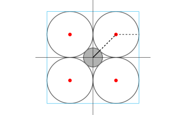
Figure 1: An arrangement of spheres as in Steele [8].

The answer is no. To see that, all we need is the multidimensional version of the Pythagorean theorem. The radius of the spheres is 1, regardless of the dimension, $n$. The length of the line between the center of a sphere and the origin is $\sqrt{n}$, so the radius of the inner sphere is $\sqrt{n}-1$. But, for $n>9$, the inner sphere must reach outside the $[-2,2]^{n}$ cube! Furthermore, as $n\to\infty$, most of the volume of the inner sphere is outside the cube.

The lesson from this example is that intuition is important for innovation, but we must not forget the first half of Poincaré’s maxim – we must do the math to prove or disprove conjectures before they can be considered discoveries.

2 A Related Question

Assume that we put a source of light at the origin. What fraction of light will be blocked by the unit balls located at vertices of the $[-1,1]^{n}$ cube? It is obvious that nothing will get out for $n=1$ and $n=2$ (see Figure 1 for $n=2$). However, when $n=3$, the collection of $2^{3}=8$ balls will allow some light out. To see this, just take a look at the structure along any axis (as can be seen in Figure 2.)

Now, before we go further, we need to provide a formal description of what we mean by the “fraction of light”. Imagine a $n-1$-dimensional hypersphere that circumscribes the n-dimensional cube $[-1,1]^{n}$. Consider all the lines that go through the origin and intersect the unit balls located at the vertices of the cube. Take those lines and intersect them with the cube circumscribing hypersphere. This set represents the shadows of those $2^{n}$ unit balls on inside of the hypersphere. Our goal is to compute the ratio of the area of the total shadow to the area of the entire hypersphere.

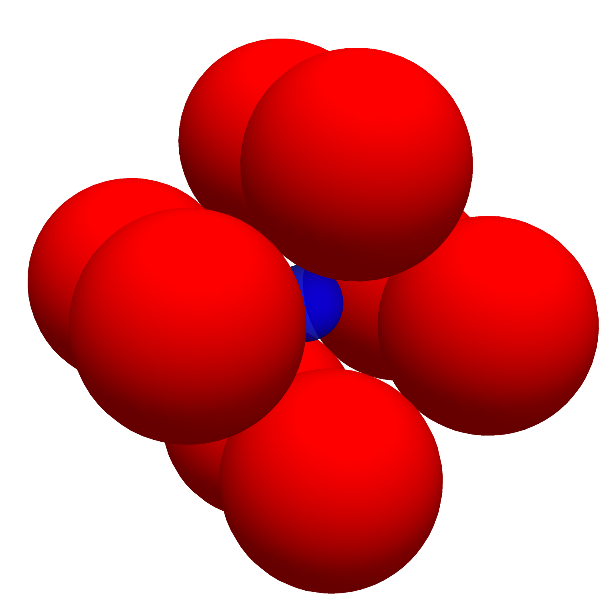
Figure 2: Arrangement of 8 unit balls in $\mathbb{R}^{3}$, centered at $\{\pm 1,\pm 1,\pm 1\}$ and a source of light emanating from the origin.

3 The Shadow of One Ball

Consider the ball of radius $0\leq r<\sqrt{n}$ located at vertex $(1,\dots,1)$. What is the area of the shadow of this one ball? The answer is known. The shadow formed by the ball is a hyperspherical cap. A cap is an nonempty intersection of a half-space and a hypersphere.

A cap can be specified in many different ways. For instance, in [1] caps are described in terms of a distance to the origin or a cap radius (see Figure 3). We will use an angle between the diagonal vector $(1,\dots,1)$ and the “edge” of the cap as it is done in [4], where a nice concise formula for the area of a cap is derived.

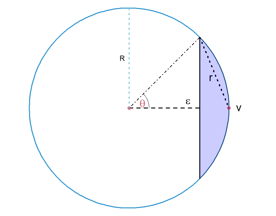
Figure 3: Definitions of a spherical cap centered at $\mathbf{v}$.

More specifically, let us consider $n-1$-dimensional hypersphere of radius $R$, denoted by $S^{n-1}(R)$. Then for any $0\leq\epsilon\leq R$, $0\leq r\leq\sqrt{R}$ and $0\leq\theta\leq\pi/2$, the smaller cap can defined as

$$C_{d}(\epsilon,\mathbf{v})=\{\mathbf{x}\in S^{n-1}(R):\mathbf{x}\cdot\mathbf{v}\geq\epsilon\},$$

or

$$C_{r}(r,\mathbf{v})=\{\mathbf{x}\in S^{n-1}(R):||\mathbf{x}-\mathbf{v}||\leq r\},$$

or

$$C_{a}(\theta,\mathbf{v})=\{\mathbf{x}\in S^{n-1}(R):\arccos(\mathbf{x}\cdot\mathbf{v})\leq\theta\},$$

where $\mathbf{x}\cdot\mathbf{v}$ is the inner product of two vectors, and $||\cdot||$ is the Euclidean distance. A simple calculation shows that when $r=2R\sin(\theta/2)$ and $\epsilon=R\cos(\theta)$, all three definitions give us the same cap.

It is well-known that the area of $n-1$-dimensional hypersphere of radius $R$ is given by

$$A_{n}(R)=\frac{2\pi^{n/2}}{\Gamma(n/2)}R^{n-1},$$ (1)

where $\Gamma(\cdot)$ is the gamma-function. It was shown in [4] that the small cap area with angle $0\leq\theta\leq\pi/2$ is given by

$$A_{n}(R,\theta)=\frac{1}{2}A_{n}(R)F\left(\sin^{2}(\theta),\frac{n-1}{2},\frac{1}{2}\right),$$ (2)

where $F$ is the cumulative distribution function (cdf) of the beta distribution:

$$F(z,\alpha,\beta)=\frac{\Gamma(\alpha+\beta)}{\Gamma(\alpha)\Gamma(\beta)}\int_{0}^{z}u^{\alpha-1}(1-u)^{\beta-1}du,\quad\quad 0<z<1,\quad\alpha,\beta>0.$$

It is easy to see that in our case the radius of the hypersphere $R=\sqrt{n}$ and $\sin^{2}(\theta)=r/n$. Therefore, the ratio of the area of the shadow to the area of the hypersphere is equal to

$$P_{n}(r)=\frac{1}{2}F\left(\frac{r}{n},\frac{n-1}{2},\frac{1}{2}\right).$$

In particular, when $n=3$ and $r=1$

$$P_{3}(1)=\frac{1}{2}\left(1-\sqrt{\frac{2}{3}}\right).$$

Since the shadow caps of 8 unit balls do not overlap the total fraction of blocked light is equal to

$$4\left(1-\sqrt{\frac{2}{3}}\right)\approx.73.$$

Moreover, one can show that the total fraction of blocked light goes to 0 as $n\to\infty$ for any fixed $r$. Indeed, we have that

$$F\left(\frac{r}{n},\frac{n-1}{2},\frac{1}{2}\right) = \frac{\Gamma(\frac{n+1}{2})}{\Gamma(\frac{n-1}{2})\Gamma(\frac{1}{2})}\int_{0}^{r/n}u^{\frac{n-1}{2}-1}(1-u)^{\frac{1}{2}-1}du$$

$$\leq \frac{\frac{n-1}{2}\Gamma(\frac{n-1}{2})}{\Gamma(\frac{n-1}{2})\Gamma(\frac{1}{2})}\int_{0}^{r/n}u^{\frac{n-3}{2}}du$$

$$= \frac{n-1}{2\sqrt{\pi}}\frac{2}{n-1}\left(\frac{r}{n}\right)^{\frac{n-1}{2}}$$

$$= \frac{1}{\sqrt{\pi}}\left(\frac{r}{n}\right)^{\frac{n-1}{2}}\,.$$

That is, the ratio of one shadow cap to $A_{n}(\sqrt{n})$ goes to 0 much faster than the number of unit balls, $2^{n}$, goes to $\infty$.

4 A More Difficult Question

It is clear that if the radii of the balls at the vertices of the cube are equal to $\sqrt{n}$, then the light will be blocked completely. So, here is a new question. Can we find $\{r_{n}\}_{n\geq 1}$ such that for $0<a<1$ we have that $P_{n}(r_{n})\to a$ as $n\to\infty$? We could not answer this question using geometry. It is not difficult to figure out an asymptotic behavior of $F\left(\frac{r_{n}}{n},\frac{n-1}{2},\frac{1}{2}\right)$ for a given sequence $\{r_{n}\}_{n\geq 1}$. But the issue is that as soon as $r_{n}>1$, the balls (and, therefore, the shadow caps) will overlap. This overlap is not easy to track, because some balls are very close to each other with the distance of 2 units between their centers, and some pairs have the distance of $2\sqrt{n}$.

Our solution is probabilistic in nature. We will use deep and important but well-known results. The first statement is about the uniform distribution on $n-1$-dimensional unit hypersphere. If we generate a vector of $n$ independent identically distributed (i.i.d.) standard normal random variables $\mathbf{Y}=(Y_{1},\dots,Y_{n})$, then

$$\frac{\mathbf{Y}}{\sqrt{Y_{1}^{2}+\cdots+Y_{n}^{2}}}$$

is uniformly distributed on surface of $n-1$-dimensional unit ball [6]. The second one is the celebrated Central Limit Theorem (CLT).

The result is quite surprising. To achieve a probability of $1/2$, the balls must be enormous. Specifically, their radii must be $\sqrt{(1-2/\pi)n}+o(1)$. Recall that the radius the cube circumscribing hypersphere is exactly $\sqrt{n}$. However, a relatively small finite variation of radii (independent of $n$) will change this probability. For example, if $r_{n}=\sqrt{(1-2/\pi)n}+1$, then the fraction of blocked light will be almost 100% for all sufficiently large $n$. And it is almost 0% for $r_{n}=\sqrt{(1-2/\pi)n}-1$.

5 Distance between a Random Line and the Nearest Vertex of the Cube $[-1,1]^{n}$

Let $\mathbf{Y}=(Y_{1},\dots,Y_{n})$ be a vector of i.i.d. standard normal random variables. Then

$$\mathbf{U}=\frac{1}{\|\mathbf{Y}\|}(Y_{1},\dots,Y_{n})$$

is a random point uniformly distributed on the unit hypersphere (here $\|\cdot\|$ is the standard Euclidean norm). We call the line associated with vector $\mathbf{Y}$, $\mathbf{y}=\mathbf{Y}t$, $t\in\mathbb{R}$, a random line.

Proposition 1.

With probability 1, the vertices

$$(\mathrm{sign}(Y_{1}),\dots,\mathrm{sign}(Y_{n}))$$

and

$$(-\mathrm{sign}(Y_{1}),\dots,-\mathrm{sign}(Y_{n}))$$

are the closest to and at the same distance from random line $\mathbf{y}=\mathbf{Y}t$, among all $2^{n}$ vertices of $C_{n}$.

Proof.

Since the distance from the origin to any vertex is the same and equal to $\sqrt{n}$, a vertex $\mathbf{v}$ with the largest absolute value of the cosine of the angle between $\mathbf{v}$ and $\mathbf{Y}$ will have the smallest distance to the random line. The absolute value of the cosine of this angle is given by

$$\frac{|\mathbf{v}\cdot\mathbf{Y}|}{\sqrt{\|\mathbf{v}\|\|\mathbf{Y}\|}}=\frac{|\mathbf{v}\cdot\mathbf{Y}|}{\sqrt{n\|\mathbf{Y}\|}}.$$

Therefore, the largest value is achieved when all the summands of inner product $\mathbf{v}\cdot\mathbf{Y}$ have the same sign. ∎

Now, let $\mathbf{X}=(X_{1},\dots,X_{n})$ be a vector of i.i.d. half-normal random variables. That is, $X_{i}$ has the same distribution as $|Z|$, where $Z$ is a standard normal random variable. Then the squared distance between a random line (passing through the origin) and the nearest vertex of the cube $[-1,1]^{n}$, denoted by $d^{2}$, is equal (in distribution) to the squared distance between point $\mathbf{c}=(1,\dots,1)$ and a line

$$\mathbf{y}=\mathbf{X}t,\quad t\in\mathbb{R}.$$

This squared distance is given by

$$d^{2}=\left\|\mathbf{c}-\frac{\mathbf{c}\cdot\mathbf{X}}{\|\mathbf{X}\|^{2}}\mathbf{X}\right\|^{2}.$$

Denote

$$s=\mathbf{c}\cdot\mathbf{X}=X_{1}+\cdots+X_{n},$$

and

$$t=\|\mathbf{X}\|^{2}=X_{1}^{2}+\cdots+X_{n}^{2}.$$

Note that $s\leq nt$. Then

$$d^{2} = \left\|\mathbf{c}-\frac{s}{t}\mathbf{X}\right\|^{2}$$

$$= \left(1-\frac{s}{t}X_{1}\right)^{2}+\dots+\left(1-\frac{s}{t}X_{n}\right)^{2}$$

$$= 1-2\frac{s}{t}X_{1}+\frac{s^{2}}{t^{2}}X_{1}^{2}+\cdots+1-2\frac{s}{t}X_{1}+\frac{s^{2}}{t^{2}}X_{1}^{2}$$

$$= n-2\frac{s}{t}s+\frac{s^{2}}{t^{2}}t$$

$$= n-\frac{s^{2}}{t}.$$

The Law of Large Numbers (LLN) immediately gives us that

$$\frac{d^{2}}{n}=1-\frac{(X_{1}+\cdot+X_{n})^{2}}{n(X_{1}^{2}+\cdots+X_{n}^{2})}=1-\frac{(X_{1}+\cdot+X_{n})^{2}}{n^{2}}\frac{n}{X_{1}^{2}+\cdots+X_{n}^{2}}\overset{\mathbf{P}}{\longrightarrow}1-\frac{2}{\pi},$$

because $\mathbf{E}(X_{i})=\sqrt{2/\pi}$ and $\mathbf{E}(X_{i}^{2})=1$. Now, let us state a general result on the asymptotic behavior of ratio $s^{2}/nt$. Note that this ratio is also the square of the cosine of the angle between random line $\mathbf{y}=\mathbf{X}t$, $t\in\mathbb{R}$ and vector $(1,\dots,1)$.

Proposition 2.

Let $\{X_{i}\}_{i\geq 1}$ be a sequence of i.i.d. positive random variables with $\mathbf{E}(X_{i})=\mu$, $\mathbf{E}(X_{i}^{2})=1$, $\mathbf{E}(X_{i}^{3})=a$, and $\mathbf{E}(X_{i}^{4})=b$. Let

$$s=X_{1}+\cdots+X_{n},$$

and

$$t=X_{1}^{2}+\cdots+X_{n}^{2}.$$

Then

$$\sqrt{n}\left[\frac{s^{2}}{nt}-\mu^{2}\right]\overset{d}{\longrightarrow}N(0,\sigma^{2}),$$

where

$$\sigma^{2}=\mu^{4}b+4\mu^{2}-4\mu^{3}a-\mu^{4}.$$

Proof.

The Central Limit Theorem (CLT) tells us that both $(s-\mu n)/\sqrt{n}$ and $(t-n)/\sqrt{n}$ are asymptotically normal. So, first note that

$$\sqrt{n}\left[\frac{s^{2}}{nt}-\mu^{2}\right] = \frac{1}{n^{3/2}}\left[s^{2}-\mu^{2}tn\right]\frac{n}{t}$$

$$= \frac{1}{n^{3/2}}\left[(s-\mu n)^{2}+2\mu ns-\mu^{2}n^{2}-\mu^{2}n(t-n)-\mu^{2}n^{2}\right]\frac{n}{t}$$

$$= \frac{1}{n^{3/2}}\left[(s-\mu n)^{2}+2\mu n(s-\mu n)-\mu^{2}n(t-n)\right]\frac{n}{t}$$

$$= \frac{1}{n^{3/2}}\left[(s-\mu n)^{2}\right]\frac{n}{t}+\frac{1}{n^{1/2}}\left[2\mu(s-\mu n)-\mu^{2}(t-n)\right]\frac{n}{t}$$

$$= \frac{1}{n^{3/2}}\left[(s-\mu n)^{2}\right]\frac{n}{t}+\frac{1}{n^{1/2}}\left[\sum_{i=1}^{n}\left(2\mu(X_{i}-\mu)-\mu^{2}(X_{i}^{2}-1)\right)\right]\frac{n}{t}\,.$$

Then, since $\mathbf{Var}(X_{i})=1-\mu^{2}$, $\mathbf{Var}(X_{i}^{2})=b-1$ and $\mathbf{Cov}(X_{i},X_{i}^{2})=a-\mu$ by the CLT we get

$$\frac{1}{n^{1/2}}\left[\sum_{i=1}^{n}\left(2\mu(X_{i}-\mu)-\mu^{2}(X_{i}^{2}-1)\right)\right]\overset{d}{\longrightarrow}N(0,\sigma^{2}).$$

But we also have that

$$\frac{1}{n^{3/2}}\left[(s-\mu n)^{2}\right]\frac{n}{t}\overset{\mathbf{P}}{\longrightarrow}0$$

and

$$n/t\overset{\mathbf{P}}{\longrightarrow}1.$$

Slutsky’s theorem is then applied to complete the proof. ∎

Now, taking into account that in our case $\mathbf{E}(X_{i})=\sqrt{2/\pi}$, $\mathbf{E}(X_{i}^{2})=1$, $\mathbf{E}(X_{i}^{3})=2\sqrt{2/\pi}$, and $\mathbf{E}(X_{i}^{4})=3$, by Proposition 2 we obtain that

$$\sqrt{n}\left[s^{2}/nt-2/\pi\right]\overset{d}{\longrightarrow}N\left(0,\frac{8}{\pi}-\frac{24}{\pi^{2}}\right).$$ (3)

Thus, the distribution of squared distance $d^{2}$ is approximately normal with mean $(1-2/\pi)n$ and standard deviation $\sqrt{(8/\pi-24/\pi^{2})n}$. A side note, the assumption $\mathbf{E}(X_{i}^{2})=1$ in Proposition 2 is not restrictive. As long as first four moments are finite, any distribution can be scaled to satisfy this assumption.

Let $\theta$ be the angle between a random line $\mathbf{y}=\mathbf{Y}t$, $t\in\mathbb{R}$ and the nearest vertex. Then by applying the delta method we obtain the following.

Corollary 1.

If $n\to\infty$, then

$$\sqrt{n}\left(\cos(\theta)-\sqrt{\frac{2}{\pi}}\right)\overset{d}{\longrightarrow}N\left(0,\frac{\pi-3}{\pi}\right),$$

and

$$d-\sqrt{\left(1-\frac{2}{\pi}\right)n}\overset{d}{\longrightarrow}N\left(0,\frac{2(\pi-3)}{\pi(\pi-2)}\right).$$

Proof.

Since $\cos^{2}(\theta)=s^{2}/nt$, applying the delta method to (3) for function $g(x)=\sqrt{x}$ we get

$$\sqrt{n}\left[g(\cos^{2}(\theta))-g\left(2/\pi\right)\right]\overset{d}{\longrightarrow}N\left(0,\left(\frac{8}{\pi}-\frac{24}{\pi^{2}}\right)\left[g^{\prime}\left(2/\pi\right)\right]^{2}\right),$$

and after some algebra we get the first asymptotic result.

Next, from (3) we also have that

$$\sqrt{n}\left[d^{2}/n-(1-2/\pi)\right]\overset{d}{\longrightarrow}N\left(0,\frac{8}{\pi}-\frac{24}{\pi^{2}}\right).$$

Therefore,

$$\sqrt{n}\left[g(d^{2}/n)-g(1-2/\pi)\right]\overset{d}{\longrightarrow}N\left(0,\left(\frac{8}{\pi}-\frac{24}{\pi^{2}}\right)\left[g^{\prime}\left(1-2/\pi\right)\right]^{2}\right),$$

which gives us the second convergence result. ∎

Corollary 1 gives us the answer to the main question of the article, which we formalize now:

Corollary 2.

Assume that at every vertex of the cube $[-1,1]^{n}$ we put a $n$-ball of radius $r_{n}$. Let $\alpha(r_{n})$ be the probability that a random line will intersect at least one of the balls. Then we have the following.

1. If $r_{n}\leq\sqrt{\alpha n}$, where $\alpha<1-2/\pi$, then $\alpha(r_{n})\to 0$ as $n\to\infty$,

2. If $r_{n}\geq\sqrt{\alpha n}$, where $\alpha>1-2/\pi$, then $\alpha(r_{n})\to 1$ as $n\to\infty$,

3. If $r_{n}=\sqrt{(1-2/\pi)n}+z\sqrt{2(\pi-3)/(\pi(\pi-2))}$, where $z\in\mathbb{R}$, then $\alpha(r_{n})\to\Phi(z)$ as $n\to\infty$, where $\Phi$ is the cdf of the standard normal distribution.

The first two statements follow from the LLN, and the last one is a consequence of the CLT.

6 Concentration of Measure

In this paper we investigate a specific question in high-dimensional geometry, and highlight some curious and perhaps surprising and non-intuitive results. Although high-dimensional geometry might appear to be a straightforward generalization of the familiar 2-D Euclidean geometry, it turns out to be a mirage. Our real-world intuition may fail us when we are trying to understand things in dimension greater than 3, and in this case it is much easier to represent the geometry symbolically, using algebra to represent geometric structures as equations in some coordinate system (usually Cartesian or polar). Still, as the dimension of the space grows, algebra alone doesn’t offer much help, since solving the equations may sometimes be impossible. In this case, we turn to probability theory which allows us to replace the quest for an exact (but infeasible) solution to an algebraic problem with a search for a distribution function which in turn, leads to the characterization of statistical properties of the solution. Finally, the distributional properties allow us to give a geometric interpretation to the solution.

We demonstrate this thought process using a simpler question. We also use this simple example to provide a clear explanation to the phenomenon known as ‘concentration of measure’.

Suppose that we get a binary-coded message of length $n$ in which each bit is $\pm 1$, and the probability of receiving 1 or -1 in each position in the message is 1/2. This can be represented geometrically as an $n$-dimensional cube, and a uniform distribution on the set of $2^{n}$ vertices, so that the probability of randomly drawing each of the $2^{n}$ vertices of the cube is $2^{-n}$. Note that all the vertices also belong to $n-1$ dimensional hypersphere of radius $\sqrt{n}$.

Now suppose that there is a reference message, which we will call a ‘pole’, and its opposite pole is obtained by multiplying $\mathbf{p}$ by $-1$. We define the $k$-th latitude

$$L_{k}=\{\mathbf{x}\in\{-1,1\}^{n}~{}:~{}||\mathbf{x}-\mathbf{p}||^{2}=4k\}\,,$$

for $k=0,1,\ldots,n$. In other words, the latitude $L_{k}$ is the set of all vertices that disagree with $\mathbf{p}$ in exactly $k$ coordinates.

When $n$ is even, $L_{n/2}$ can be called ‘equator’, because it is the set of points that are at the same distance from $\mathbf{p}$ and $-\mathbf{p}$. It is easy to see that the points in the equator are perpendicular to the pole $\mathbf{p}$. Indeed, $\mathbf{x}\in L_{n/2}$ if exactly $n/2$ of its coordinates are the same as in $\mathbf{p}$. Therefore, $\mathbf{p}\cdot\mathbf{x}=0$, that is, the cosine of the angle between $\mathbf{p}$ and $\mathbf{x}$ is 0.

A randomly chosen vertex falls in the $k$-th latitude relative to the pole with probability $p(k)$, which follows the binomial distribution with $n$ trials and probability of success 1/2. This is so because, being in the $k$-th latitude is equivalent to choosing $k$ coordinates in $\mathbf{p}$ and multiplying them by $-1$. If we denote the latitude relative to $\mathbf{p}$ in which a random vertex falls by $K$, then the expected value of the latitude is $\mathbf{E}(K)=n/2$ and the variance is $\mathbf{Var}(K)=n/4$. Therefore, Bernoulli’s LLN for the binomial distribution tells us that for any (small) $\epsilon>0$ and sufficiently large $n$, with probability close to 1 the latitude of the random vertices will be within $\epsilon n$ distance from $n/2$. Of course, similarly to our Corollary 2, the CLT will give us even more precise statement.

Thus, for large $n$, the thin central slab of the hypersphere $S^{n-1}(\sqrt{n})$ contains almost all random vertices. Alternatively, we can say that almost all random vertices lie outside two large caps centered at two opposite poles $\mathbf{p}$ and $-\mathbf{p}$. Considering that our choice of poles is arbitrary, this statement is also correct for any other central slab. Try to use our 3-D intuition to visualize these two statements! This is known as the “concentration of measure phenomenon”. There is a deep connection between the concentration of measure and the Law of Large Numbers (LLN) for independent random variables. This connection is the main topic of Talagrand’s seminal paper[9].

In fact, with a bit of effort, one can show that Proposition 2.1 of [9] is directly applicable to our situation. Essentially, it states that if we select any subset $A$ of the vertices such that $\mathbf{P}(A)\geq 1/2$ , then most of the remaining vertices will be close to $A$ . This implies that if we take a hemisphere with pole $\mathbf{p}$ (including the equator if $n$ is even), then with high probability, the rest of the vertices will be close to this set, meaning they will belong to a thin slab right under the hemisphere. Since the same is true for the opposite hemisphere with pole $-\mathbf{p}$, we obtain the same result as before: with high probability, a random vertex belongs to a thin central slab. However, this “proof” is based on the concentration of measure, not the Law of Large Numbers. Also note that, as before, the same can be derived for hemispheres with different opposing poles.

Consider what this means in the context of receiving a binary-coded message, such as ones transmitted by GPS satellites. If there is no prior information and we do not know what message is expected, each sequence of length $n$ is equally likely. But, if we expect a specific message $\mathbf{p}$ (e.g., the identifier of a specific satellite), then the vast majority of random messages will be nearly perpendicular to $\mathbf{p}$, making it very easy to detect them as noise. In contrast, a message with few errors will be in a latitude far enough from the equator, and close to the cap centered at $\mathbf{p}$. This is what may be referred to as ‘the blessing of dimensionality’.

Importantly, concentration of measure in high dimensional spaces arises as a result of choosing reference points. Data that are distributed uniformly without such points, become tightly concentrated in very specific regions which depend on our choice of poles or reference points.

7 Discussion

Is high dimensional data a blessing or a curse? Clearly, it presents significant challenges, both theoretical and computational. It is also impossible to visualize or to obtain geometrical interpretations for such data. It is tempting to assume that our intuition in the two dimensional Euclidean space extends to higher dimensions, but this is not so. However, through probability models one can derive asymptotic results and obtain a geometric intuition, which is often surprising, if not counterintuitive. In particular, high-dimensional data tends to concentrate at very specific regions which depend on our choice of coordinate system and reference points. For example, relative to a point of origin, multivariate normal distribution in $\mathbb{R}^{n}$ concentrates very close to a sphere of radius $\sqrt{n}$, and if one chooses two points as opposing poles on the sphere, then the data concentrates near the equator relative to the poles. In both cases, the $\sqrt{n}$-sphere and the central slab are both very big regions, but much smaller than the $n$-dimensional ball of radius $\sqrt{n}$. We highlight the deep connection between concentration of measure and the law of large numbers for independent random variables. We also discuss why the fact that in high dimension, independent random data is highly concentrated, is actually a blessing.

In the discrete example discussed in Section 6 the random vectors are drawn uniformly from the set of $2^{n}$ cube vertices. In our paper we assume that an $n$-dimensional random vector comes from a standard multivariate normal distribution. The support is the entire Euclidean space, but most of the drawn data are concentrated very close to the sphere of radius $\sqrt{n}$. This is so because, although the expected location of a random univariate normal variable $x$ is 0, its expected length is $1$ (the length is $|x_{i}|=\sqrt{x_{i}^{2}}$, which has a half-normal (or a chi) distribution.) The sum of $n$ independent squared standard normal random variables has a chi-squared distribution with $n$ degrees of freedom, with mean $n$. Thus, using the CLT, one can show that random multivariate normal data is concentrated close to the sphere of radius $\sqrt{n}$. The origin of this famous result is discussed in [6] which highlights Lévy’s contributions. Lévy’s [5] motivation was a 1914 paper by Borel [2] who made a remark about geometric interpretation of the law of large numbers, but the result was even known to Poincaré in 1912 [7].

References

- [1] Keith Ball. An elementary introduction to modern convex geometry. Flavors of geometry, 31:1–58, 1997.
- [2] Emile Borel. Introduction géométrique à quelques théories physiques. Gauthier-Villars, Paris, 1914.
- [3] M. Gardner. Aha! Gotcha: Paradoxes to Puzzle and Delight. Tools for Transformation. W.H. Freeman, 1982.
- [4] S. Li. Concise formulas for the area and volume of a hyperspherical cap. Asian J. Math. Stat., 4(1):66–70, 2011.
- [5] P. Lévy. Problèmes Concrets d’Analyse Fonctionnelle. Gauthier-Villars, Paris, 1951.
- [6] V. D. Milman. The heritage of P. Lévy in geometrical functional analysis. In Astérisque, volume 157-158, pages 273–301, 1988.
- [7] H. Poincaré. Calcul des probabilities. Gauthier-Villars, Paris, 1912.
- [8] J. Michael Steele. The Cauchy-Schwarz master class. AMS/MAA Problem Books Series. Mathematical Association of America, Washington, DC; Cambridge University Press, Cambridge, 2004. An introduction to the art of mathematical inequalities.
- [9] Michel Talagrand. A new look at independence. Ann. Probab., 24(1):1–34, 1996.
- [10] Gary L Wise and Eric B Hall. The Counter examples. In Counterexamples in Probability and Real Analysis. Oxford University Press, 10 1993.