Tripartite entanglement from experimental data:
$B^{0}\to K^{*0}\mu^{+}\mu^{-}$ as a case study

Roberto A. Morales^aand Alejandro Szynkman^a

^aIFLP, CONICET - Dpto. de Física, Universidad Nacional de La Plata,
C.C. 67, 1900 La Plata, Argentina

Abstract

We develop an angular analysis based on the reconstruction of the helicity amplitudes from dedicated experimental data corresponding to the tripartite state composed by one qutrit and two qubits, which arises in the three-body decays of a spin zero particle into one vector and a fermion pair. Starting from the associated spin density matrix of the final state, entanglement quantifiers were investigated and the corresponding significances were determined up to second order in the error propagation of the uncertainties of the angular measurements. As an application of our analysis, we performed a full quantum tomography of the final state in the $B^{0}\to K^{*0}\mu^{+}\mu^{-}$ decays using data recorded by LHCb collaboration. We found the presence of genuine quantum entanglement of the final state and also in both kaon-muon and di-muon subsystems. In recent years, $B$ meson decays received significant attention from both experimental and theoretical sides, and the proposed observables provide novel perspectives for studying them. Furthermore, this analysis could be also applied to other several processes if the complete experimental data were available for the helicity amplitudes reconstruction.

1 Introduction

As a fundamental concept in Quantum Mechanics, the quantum entanglement between the constituents of a multipartite system represents the strong correlations among them that cannot be explained by local realism. In particular, the state of a subsystem cannot be independently described without considering the rest of the complete system, despite of their physical separation. The ultimate consequence of this property is the violation of the Bell inequality [1]. Theoretical aspects of entanglement and Bell nonlocality can be found in reviews [2, 3]. Furthermore, the manipulation, control and distribution of the entanglement in a given system is the key ingredient for applications such as cryptography [4], teleportation [5] and quantum computation [6].

Historically, quantum entanglement and the violation of Bell inequality were widely studied in photonic, atomic and even macroscopic systems via electromagnetic forces [7, 8, 9, 10, 11, 12, 13]. In the recent years, the high-energy physics (HEP) community revealed the interest for studying it at particle colliders, such as the LHC (see, for instance, a recent review [14]). In fact, ATLAS and CMS collaborations observed entanglement between the top quark spin in $t\bar{t}$ production with a significance larger than 5$\sigma$ [15, 16, 17], as it was studied in [18, 19, 20, 21, 22, 23, 24, 25]. Other interesting systems with two elementary particles correspond to the final state in the Higgs boson decays into a tau-lepton pair, two photons and photon plus $Z$ boson [26, 27, 28, 29], into massive gauge bosons [30, 31, 32, 33, 34, 35, 36], and also to the final state in $b\bar{b}$ [37]. Diboson production at LHC [34, 33, 38, 39] and vector boson scattering [40] were considered too. More related to this work, neutral meson oscillations [41, 42, 43, 44], for which an indirect test of Bell inequality violation in $B\bar{B}$ was reported by Belle collaboration [45], and charmonium systems [46, 47, 48, 49, 50, 51] were also studied.

Particularly relevant for the present analysis are [52, 53, 54, 55], in which experimental data were used as input to compute entanglement between the spin degrees of freedom of the final particles in two-body $B$ meson decays. A natural extension of these previous works is to move towards tripartite entanglement. In this work we focus on three-body decays, where the final state is made of one massive vector ($V$) and two spin $1/2$ fermion particles ($f^{+}f^{-}$ pair), which correspond to a system of one qutrit and two qubits in the Quantum Information language. Even if in principle the decaying state could have any spin consistent with angular momentum conservation, the density matrix obtained in this paper is only valid for a spin $0$ particle. Of course, there are many decays of such particles with the specific final state under interest. Among the ones commented in Section 2, which include mesons or baryons in the final state, we center on semi-leptonic $B$ meson decays mediated by one-loop transitions. In particular, we analyze the $B^{0}\to K^{*0}\mu^{+}\mu^{-}$ decays which, as far as we know, are the only ones where a complete experimental angular analysis is available. It should be pointed out that tripartite entanglement in the HEP context is less explored than the bipartite case. In particular, a general description of the spin in multipartite systems were presented in [56, 57]. Furthermore, positronium decaying into three photons [58], three-flavor entanglement in neutrino oscillations [59, 60], spectator particle in QED processes [61, 62, 63], heavy fermion decays to three fermions through generic (pseudo)scalar, (pseudo)vector and (pseudo)tensor interactions [64], spin and total angular momentum entanglement in $H\to ZZ,WW$ [65], one-loop Higgs boson decay into a photon and a lepton pair [29], and $t\bar{t}Z$ production at LHC [66] were previously studied.

To the best of our knowledge, this work presents the first analysis of tripartite entanglement of a process that combines non-perturbative QCD effects and EW interactions. Then these decays provide a unique opportunity to test fundamental interactions through the novel application of observables which exploit the spin correlations between the final state particles $V$, $f^{+}$ and $f^{-}$. This information comes from the helicity amplitudes which can be reconstructed from experimental data through angular coefficients that describe these decays. In particular, there is a lot of information in the three-body final state that depends on the kinematics. Hence we need the complete set of observables that defines the resulting spatial configuration. Many experimental searches provide partial information that in general corresponds to differential branching ratios, CP and forward-backward asymmetries, polarization factors, some particular optimised angular observables and those related to lepton flavor universality tests. Our aim is to fulfil a quantum tomography of the tripartite system, i.e. reconstruct the spin density matrix of the final decay products from experimental data.

Flavour changing neutral currents (FCNC) are forbidden at tree-level in the Standard Model (SM), leading to tiny expected amplitudes. The one-loop $b\to ql^{+}l^{-}$ transitions ($q=d,s$ and $l=e,\mu,\tau$) occur via suppressed topologies such as electroweak penguins. Hence these rare decays offer the great opportunity to test physics beyond the Standard Model that may couple to quarks and leptons. As mentioned, we consider the $B^{0}\to K^{*0}\mu^{+}\mu^{-}$ decays as a leading case for the study of tripartite entanglement through the evaluation of relevant observables directly from experimental data. From this novel perspective, the present analysis probes its quantum properties and makes use of the CP-averages and CP-asymmetries. An intense program of measurements of the angular observables of this decay was carried out by the Babar [67, 68], CDF [69], Belle [70, 71], LHCb [72, 73, 74, 75, 76], ATLAS [77] and CMS [78, 79] collaborations (see also the recent LHCb reviews [80, 81, 82]). Along with the $B\rightarrow K\mu^{+}\mu^{-}$ decay, $B^{0}\to K^{*0}\mu^{+}\mu^{-}$ has received particular attention in the last few years due to the presence of discrepancies from the SM predictions in some observables. Deviations of $2.3\sigma$ and $2.5\sigma$ in the lepton universality ratio $R_{K*}$ in two kinematical regions displaying a suppression compared to the SM [83], together with a $3\sigma$ discrepancy in the same direction in the analogous ratio ($R_{K}$) for the decay $B^{+}\to K^{+}\mu^{+}\mu^{-}$ [84], had opened expectations for finding new physics (NP) in decays mediated by the $b\rightarrow s\mu^{+}\mu^{-}$ transition. However, more recent measurements made the ratios consistent with the SM at $1\sigma$ [85, 86]. Even then, measurements from LHCb and CMS still show deviations in the branching ratio $BR(B\to K\mu^{+}\mu^{-})$ [87, 88, 89, 90] and $P^{\prime}_{5}$($B\rightarrow K^{*}\mu^{+}\mu^{-}$) at large recoil [91, 76, 78, 71, 77]. Despite of the remarkable progress in the theoretical predictions of these semi-leptonic rare decays, no conclusive findings regarding NP can be drawn since we still have limited precision in both experimental measurements and theoretical computations. In view of this, although the study of the impact of the observables analyzed here on the search of NP is beyond the scope of this article, they might also offer an alternative way to explore new physics in a decay sensitive to small non-standard effects.

The paper is structured as follows: an overview of the helicity amplitudes treatment for $B\to Vl^{+}l^{-}$ decays is given in Section 2. Particular attention to how reconstruct them in terms of experimental data is focused here. Section 3 introduces the tripartite entanglement quantifiers relevant for our analysis. The results corresponding to $\bar{B}^{0}\to\bar{K}^{*0}\mu^{+}\mu^{-}$ at second order in the error propagation and a correspondence with previous literature are presented in Section 4. Finally, Section 5 summarize the main findings and outline future perspectives. Appendices collect the numerical results and provide details and generalizations of the implemented statistical analysis.

2 Three-body $B$ meson decays

We will derive the quantum entanglement between the spin degrees of freedom of the final particles in the processes $B^{0}\to K^{*0}l^{+}l^{-}$ and $\bar{B}^{0}\to\bar{K}^{*0}l^{+}l^{-}$. That is, we consider a $B^{0}$ ($\bar{B}^{0}$) meson decaying into an on-shell $K^{*0}$ ($\bar{K}^{*0}$) and a virtual photon or $Z$ boson with subsequent decay into a di-lepton pair. The spin along the direction of motion of $K^{*0}$ ($\bar{K}^{*0}$), antilepton and lepton are $s_{1}$, $s_{2}$ and $s_{3}$, respectively. These final states corresponds to a system of one qutrit and two qubits and they are expanded using the helicity amplitude basis $\{+,0,-\}\otimes\{+,-\}\otimes\{+,-\}$. In this section, we will present a summary of the helicity amplitudes treatment of these decays, based on [92, 93]. Assuming massless leptons and in the absence of scalar and pseudoscalar operators, the total amplitude can be written in terms of six non-vanishing helicity amplitudes $\bar{\mathcal{H}}_{s_{1}s_{2}s_{3}}$ ($\mathcal{H}_{s_{1}s_{2}s_{3}}$) and the pure final state $|\psi\rangle$ is expanded as

$$|\psi\rangle=\mathcal{H}_{++-}|++-\rangle+\mathcal{H}_{+-+}|+-+\rangle+\mathcal{H}_{0+-}|0+-\rangle+\mathcal{H}_{0-+}|0-+\rangle+\mathcal{H}_{-+-}|-+-\rangle+\mathcal{H}_{--+}|--+\rangle$$ (2.1)

Hence, the resulting 12$\times$12 spin density matrix $\rho=|\psi\rangle\langle\psi|$ is constructed as

$$\langle s_{1}\,s_{2}\,s_{3}|\rho|s^{\prime}_{1}\,s^{\prime}_{2}\,s^{\prime}_{3}\rangle=\left(\sum_{s_{1},s_{2},s_{3}}|\mathcal{H}_{s_{1}s_{2}s_{3}}|^{2}\right)^{-1}\mathcal{H}_{s_{1}s_{2}s_{3}}\mathcal{H}^{\dagger}_{s^{\prime}_{1}s^{\prime}_{2}s^{\prime}_{3}}$$ (2.2)

where the first factor in the r.h.s is the total unpolarized square amplitude and determines the normalization Tr[$\rho$]=1.

In particular, the $|-+\rangle$ and $|+-\rangle$ di-lepton subsystem helicity states correspond to the Left and Right lepton currents coupled to the virtual gauge bosons, whereas $|++\rangle$ and $|--\rangle$ states do not contribute in this massless lepton case. It is convenient to introduce the transversity amplitudes as follows,

$$\mathcal{A}^{L(R)}_{\perp} = \left(\mathcal{H}_{+-+(++-)}-\mathcal{H}_{--+(-+-)}\right)/\sqrt{2}$$

$$\mathcal{A}^{L(R)}_{\parallel} = \left(\mathcal{H}_{+-+(++-)}+\mathcal{H}_{--+(-+-)}\right)/\sqrt{2}$$

$$\mathcal{A}_{0}^{L(R)} = \mathcal{H}_{0-+(0+-)}$$ (2.3)

From the theoretical side, these decays receive two kind of contributions, local and nonlocal [94, 95, 96]. The first ones are formulated in terms of a local operator expansion and might encode the presence of NP. The nonlocal contributions are dominated by narrow charmonium resonances in the di-lepton mass squared ($q^{2}$) spectrum but affect the whole phase space. These decays are described by the Weak Effective Theory framework, see for instance [92], where the effective operators and the associated couplings (Wilson coefficients) account for long- and short-distance effects when all heavy particles are integrated out. Within the SM, the effective Hamiltonian is dominated by ten operators with a chirality structure which arises from the axial-vector pattern of the weak interactions. The decay amplitudes depend on calculations of several non-perturbative hadronic matrix elements. The associated local form factors are computed in lattice QCD (LQCD) and light-cone sum rules (LCSR). Nevertheless, the nonlocal contributions are less understood and faithful computations with controlled uncertainties are not yet available. Concretely, they are associated to the four-quark operators leading to the $b\to sc\bar{c}$ transition with subsequent $c\bar{c}\to\gamma^{*}\to l^{+}l^{-}$ process mediated by the electromagnetic current. The relevance and influence of the nonlocal contributions are under debate in recent years. Comprehensive state-of-the-art overviews of local and nonlocal contributions in the $B^{0}\to K^{*0}\mu^{+}\mu^{-}$ decays are presented in [82, 97]. In order to compare with the values obtained from the experimental data, we also compute in this work the SM predictions of the entanglement quantifiers using the FLAVIO package [98]. For illustrative purposes, we focus on the low-$q^{2}$ regime within the energy range $1.1<q^{2}<4m_{c}^{2}\sim 6$ GeV², where the theoretical predictions are more reliable. In particular, the lower bound guarantees the massless electron and muon assumption and evades the photon-pole peaked distribution. On the other hand, the upper bound provides a safe framework to estimate the charm-loop effect.

From the experimental side, the present decays were observed at colliders for electron and muon pairs [67, 68, 69, 70, 71, 72, 73, 74, 75, 76, 77, 78, 79]. However the electron case is harder to reconstruct at hadron colliders, and the tau case is so difficult to reconstruct at any experiment that it has not been observed yet. The experimental analysis focus in the mass shell subsequent decays $K^{*0}\to K^{+}\pi^{-}$ and $\bar{K}^{*0}\to K^{-}\pi^{+}$, respectively. In particular, the angle between $K^{\pm}$ and $\pi^{\mp}$ provides the additional information needed for the $K^{*0}$ and $\bar{K}^{*0}$ polarizations. The final states are completely described by four independent kinematical variables: $q^{2}$, invariant mass squared of the di-lepton system, and $\vec{\Omega}=(\cos\theta_{l},\cos\theta_{K^{*}},\phi)$, solid angle specified in Appendix A of Ref. [72] (see also [92, 93, 99, 100]). Summing over final spin particles, the differential partial width of $\bar{B}^{0}\to\bar{K}^{*0}l^{+}l^{-}$ is

$$\frac{32\pi}{9}\frac{d\Gamma}{dq^{2}d\vec{\Omega}} = J_{1s}\sin^{2}\theta_{K^{*}}+J_{1c}\cos^{2}\theta_{K^{*}}+\left(J_{2s}\sin^{2}\theta_{K^{*}}+J_{2c}\cos^{2}\theta_{K^{*}}\right)\cos 2\theta_{l}$$ (2.4)

$$+J_{3}\sin^{2}\theta_{K^{*}}\sin^{2}\theta_{l}\cos 2\phi+J_{4}\sin 2\theta_{K^{*}}\sin 2\theta_{l}\cos\phi$$

$$+J_{5}\sin 2\theta_{K^{*}}\sin\theta_{l}\cos\phi+\left(J_{6s}\sin^{2}\theta_{K^{*}}+J_{6c}\cos^{2}\theta_{K^{*}}\right)\cos\theta_{l}$$

$$+J_{7}\sin 2\theta_{K^{*}}\sin\theta_{l}\sin\phi+J_{8}\sin 2\theta_{K^{*}}\sin 2\theta_{l}\sin\phi+J_{9}\sin^{2}\theta_{K^{*}}\sin^{2}\theta_{l}\sin 2\phi$$

where the 12 angular coefficients $J_{i}$ just depend on $q^{2}$ and are related to the six complex transversity amplitudes of Eq. (2.3) in a non-trivial way [92, 93]. The CP-conjugated partial width decay, $\bar{\Gamma}(B^{0}\to K^{*0}l^{+}l^{-})$, is obtained from the previous expression taking all weak phases conjugated. Under the present conventions, this transformation yields

$$J_{1s,1c,2s,2c,3,4,7}\to\bar{J}_{1s,1c,2s,2c,3,4,7}\quad\text{and}\quad J_{5,6s,6c,8,9}\to-\bar{J}_{5,6s,6c,8,9}$$ (2.5)

In addition, three conditions arise in the present massless lepton and no scalar operators case:

$$J_{1s}=3J_{2s}\,,\quad J_{1c}=-J_{2c}\quad\text{and}\quad J_{6c}=0\,,$$ (2.6)

and quantities are normalized respect to the partial width, which in that case is

$$\frac{d\Gamma}{dq^{2}} = |\mathcal{A}_{0}^{L}|^{2}+|\mathcal{A}_{0}^{R}|^{2}+|\mathcal{A}^{L}_{\perp}|^{2}+|\mathcal{A}^{R}_{\perp}|^{2}+|\mathcal{A}^{L}_{\parallel}|^{2}+|\mathcal{A}^{R}_{\parallel}|^{2}$$ (2.7)

$$= J_{1c}+4J_{1s}/3$$ (2.8)

Concretely, these angular coefficients are all physical observables and contain the complete extracted information from experiment through the CP-averages ($S_{i}$) and CP-asymmetries ($A_{i}$), defined in the following way

$$J_{i}=\frac{S_{i}+A_{i}}{2}\frac{d(\Gamma+\bar{\Gamma})}{dq^{2}}\quad\text{and}\quad\bar{J}_{i}=\frac{S_{i}-A_{i}}{2}\frac{d(\Gamma+\bar{\Gamma})}{dq^{2}}$$ (2.9)

In order to extract information from experiments, it is convenient to introduce the fraction of longitudinal polarization of the $K^{*0}$ mesons as

$$F_{L}=S_{1c}$$ (2.10)

and, with this definition in the normalization condition of Eq. (2.8), we have $S_{1s}=3(1-F_{L})/4$. Other commonly measurements are the CP and forward-backward (FB) asymmetries in the di-lepton mass distributions

$$A_{CP}=A_{1c}+4A_{1s}/3\quad\text{and}\quad A_{FB}=3S_{6s}/4$$ (2.11)

Hence, we extract from collider data the following 8 CP-averages and 8 CP-asymmetries

$$F_{L}\,,\,\,S_{3}\,,\,\,S_{4}\,,\,\,S_{5}\,,\,\,A_{FB}\,,\,\,S_{7}\,,\,\,S_{8}\,,\,\,S_{9}\,\,\text{and}\,\,A_{CP}\,,\,\,A_{3}\,,\,\,A_{4}\,,\,\,A_{5}\,,\,\,A_{6}\,,\,\,A_{7}\,,\,\,A_{8}\,,\,\,A_{9}$$ (2.12)

The key for this analysis is to reconstruct the helicity amplitudes from the experimental measurements corresponding to these CP-averages and CP-asymmetries. The formalism was developed in [93]: for the massless lepton case without scalar operator, we have 6 complex helicity amplitudes (12 real degrees of freedom) and 4 internal symmetries for $\bar{B}^{0}\to\bar{K}^{*0}l^{+}l^{-}$, and the same holds for $B^{0}\to K^{*0}l^{+}l^{-}$. Hence, each decay is described by 8 real degrees of freedom and, following Eq. (2.9), supposes the knowledge of the 16 observables $S_{i}$ and $A_{i}$. In terms of the angular coefficients, the helicity amplitudes are derived by

$$\mathcal{A}^{L}_{\parallel} = 0\,,$$

$$\mathcal{A}^{R}_{\parallel} = \sqrt{\left|\frac{2}{3}J_{1s}-J_{3}\right|}\,,$$

$$\mathcal{A}^{R}_{\perp} = -\frac{J_{6s}-2iJ_{9}}{2\sqrt{\left|\frac{2}{3}J_{1s}-J_{3}\right|}}\,,$$

$$\mathcal{A}_{0}^{R} = \frac{2J_{4}-iJ_{7}}{\sqrt{2\left|\frac{2}{3}J_{1s}-J_{3}\right|}}\,,$$

$$|\mathcal{A}^{L}_{\perp}| = \sqrt{\left|\frac{\frac{4}{9}J_{1s}^{2}-J_{3}^{2}-\frac{1}{4}J_{6s}^{2}-J_{9}^{2}}{\frac{2}{3}J_{1s}-J_{3}}\right|}\,,$$

$$|\mathcal{A}_{0}^{L}| = \sqrt{\left|\frac{J_{1c}(\frac{2}{3}J_{1s}-J_{3})-2J_{4}^{2}-\frac{1}{2}J_{7}^{2}}{\frac{2}{3}J_{1s}-J_{3}}\right|}\,,$$

$$e^{i(\phi^{L}_{\perp}-\phi_{0}^{L})} = \frac{J_{5}(\frac{2}{3}J_{1s}-J_{3})-J_{4}J_{6s}-J_{7}J_{9}-i(\frac{4}{3}J_{1s}J_{8}-2J_{3}J_{8}+2J_{4}J_{9}-\frac{1}{2}J_{6s}J_{7})}{\sqrt{\left|2(\frac{4}{9}J_{1s}^{2}-J_{3}^{2}-\frac{1}{4}J_{6s}^{2}-J_{9}^{2})(J_{1c}(\frac{2}{3}J_{1s}-J_{3})-2J_{4}^{2}-\frac{1}{2}J_{7}^{2})\right|}}$$ (2.13)

In particular, two internal symmetries make $\mathcal{A}^{L}_{\parallel}$ equals to zero ($|\mathcal{A}^{L}_{\parallel}|=\phi^{L}_{\parallel}=0$). The third symmetry allows to take $\mathcal{A}^{R}_{\parallel}$ real ($\phi^{R}_{\parallel}=0$). The fourth one sets $\phi_{0}^{L}$ in order to have $\mathcal{A}_{0}^{L}$ real. Using the relation $A_{1c}=A_{CP}-4A_{1s}/3$, this fourth internal symmetry also determines a cubic equation for $A_{1s}$ after imposing unit modulus in the last line of Eq. (2.13). In general, this cubic equation has one real solution and we can univocally recover the angular coefficients $J_{i}$ and $\bar{J}_{i}$ from the CP-averages and CP-asymmetries using the 16 measurements of Eq. (2.12). We refer to non-degenerated case when the cubic equation has one real solution. In other words, the full differential partial width in Eq. (2.4) does not uniquely determine the helicity amplitudes since some information is lost after summing over the final lepton spins and ambiguities arise in the solutions [100]. A detailed treatment of these ambiguities is beyond the scope of this work and we separately treat the degenerated cases, corresponding to three real solutions of the cubic equation.

Therefore, the 8 real degrees of freedom of the non-vanishing amplitudes are

$$|\mathcal{A}^{R}_{\parallel}|\,,\,\,|\mathcal{A}^{L}_{\perp}|\,,\,\,|\mathcal{A}^{R}_{\perp}|\,,\,\,|\mathcal{A}_{0}^{L}|\,,\,\,|\mathcal{A}_{0}^{R}|\,,\,\,\phi^{L}_{\perp}\,,\,\,\phi^{R}_{\perp}\,\,\text{and}\,\,\phi_{0}^{R}$$ (2.14)

and they can be recovered from experimental data given in Eq. (2.12) in order to fulfil a quantum tomography for these decays.

The previous analysis also applies to other processes where a spin $0$ particle decays into a final state with one massive spin $1$ and two spin $1/2$ particles. This is due to the fact that all these decays share the disintegration differential rate shown in Eq. (2.4). In the following we comment about decays which could be subject to an equivalent analysis but, to the best of our knowledge, such a possibility is not feasible because not all the required experimental information is available. In particular, the charged decays, $B^{\pm}\to K^{*\pm}\mu^{+}\mu^{-}$, are the closest to the ones studied in this work. However, it is not possible to obtain the density matrix since published data on the $CP$-asymmetries is not attainable. Instead, the most complete study so far involves $CP$-averaged angular observables [101, 91]. Other similar decays are $B\to K^{*}e^{+}e^{-}$ however, due to the presence of electrons in the final state, the experimental analysis is even more demanding and some of the necessary information is lacking as well. Concretely, the corresponding analyses were devoted to constraint the photon polarization in $b\to s\gamma$ transition from these decays, focusing in the very low dielectron invariant mass [102, 103], where the virtual photon is then quasi-real. Additional close related decays are $B\to K^{*}\tau^{+}\tau^{-}$. However, the reconstruction of taus in the final state makes this channel specially challenging and just an upper limit on its branching ratio was reported in [104]. Other semi-leptonic $B$ decays that could be analyzed are $B\to\rho\mu^{+}\mu^{-}$ and $B\to a_{1}\mu^{+}\mu^{-}$. Baryon modes as, for instance, $B\to K^{*}p\bar{p}$ and $B\to K^{*}\Lambda\bar{\Lambda}$, may be also studied. Nevertheless, the angular information is not available for none of the previous decays. It would be also possible to consider $B$ decays into heavier resonances as, for instance, $K_{1}$ and excited $K^{*}$ states but these are even less accessible experimentally. $B_{s}$ decays could be analyzed within the same framework too. In particular, for the $B_{s}\to\phi\mu^{+}\mu^{-}$ decay an analysis of the angular distributions of the final state has been performed [105, 106]. However, the limitation in this case is related to the fact that this decay is not flavor-specific. Finally, $B_{c}$($D$) mesons decaying into a $D^{*}_{s}$($\rho,\phi,\omega$) and a pair of muons or electrons of opposite sign could be also analyzed but the corresponding experimental angular analyses would be needed.

Before concluding this section, and with the aim to facilitate a broader background for the reader, we would like to remark the considerable effort to study from a phenomenological perspective the decay analyzed in this paper, $B^{0}\to K^{*0}\mu^{+}\mu^{-}$, just as the ones discussed in the previous paragraph. See, for instance, [107, 108, 109, 110, 111, 112, 113, 114, 115, 116, 117, 118, 119, 120, 121, 122, 123, 124, 125, 126, 127, 128, 129, 130, 131, 132, 133, 134, 135, 136, 137, 138, 139] and references therein.

3 Tripartite Entanglement

Our aim is to quantify the entanglement for the multipartite quantum states $K^{*0}l^{+}l^{-}$ in Eq. (2.2). Following [64, 56, 29], we will compute the one-to-other concurrences, associated to partial separability, as

$$\mathcal{C}_{jk|i}=\sqrt{2(1-{\rm Tr}[\rho_{jk}^{2}])}\,,$$ (3.1)

where $\rho_{jk}$ is the reduced density matrix of subsystem $jk$ by tracing over particle $i$, i.e. $\rho_{jk}={\rm Tr}_{i}[\rho]$. The relevance of this quantifier is that a state described by $\rho$ is biseparable if and only if $\mathcal{C}_{jk|i}=0$.

The so-called genuine separability is a direct generalization of the bipartite entanglement vs. separability criteria [140, 2]. In that case, the system results entangled respect to all bipartitions of the parties. Then we construct the concurrence triangle with previous one-to-other concurrences and the resulting area represents a measure of the genuine tripartite entanglement (GTE) of this final state, which is given by

$$\mathcal{F}_{3}=\sqrt{\frac{16}{3}S(S-\mathcal{C}_{23|1})(S-\mathcal{C}_{31|2})(S-\mathcal{C}_{12|3})}\,,$$ (3.2)

where $S=(\mathcal{C}_{23|1}+\mathcal{C}_{31|2}+\mathcal{C}_{12|3})/2$ is the semiperimeter of the concurrence triangle [141].

Beyond the entanglement due to correlations among constituents of a system, it is the concept of non-locality. At experimental level, Quantum Mechanics (QM) and local realistic (LR) or hidden variable (LHV) theories can be discriminated via Bell inequalities [1], which can be violated just by QM predictions. In the multipartite case, non-locality has a more complex structure and its characterization results in a very hard problem. Concretely, there exist different concepts of non-locality as extensions of the bipartite definition [3]. For 2-qubit systems, the Clauser-Horne-Shimony-Holt (CHSH) [142] is the unique relevant (optimal) Bell operator. For more than two qubits, Mermin [143] and Svetlichny [144] operators act as discriminators between QM and LR predictions. However, as far as we know, there is not such Bell operators for the mixed case of one qutrit and two qubits. Therefore, we do not pursue this issue in this work.

Next, we analytically compute the concurrences defined in Eq. (3.1) for the three bipartitions of the final state in the $\bar{B}^{0}\to\bar{K}^{*0}l^{+}l^{-}$ decay, assuming massless leptons and no scalar nor pseudoscalar operator contributions. We found that

$$\mathcal{C}_{\bar{K}^{*}l^{+}|l^{-}} = \mathcal{C}_{\bar{K}^{*}l^{-}|l^{+}}=2\left(\frac{d\Gamma}{dq^{2}}\right)^{-1}\left(|\mathcal{A}_{0}^{L}|^{2}+|\mathcal{A}^{L}_{\perp}|^{2}+|\mathcal{A}^{L}_{\parallel}|^{2}\right)^{1/2}\left(|\mathcal{A}_{0}^{R}|^{2}+|\mathcal{A}^{R}_{\perp}|^{2}+|\mathcal{A}^{R}_{\parallel}|^{2}\right)^{1/2}$$

$$\mathcal{C}_{l^{-}l^{+}|\bar{K}^{*}} = 2\left(\frac{d\Gamma}{dq^{2}}\right)^{-1}\left(|\mathcal{A}_{0}^{L}|^{2}|\mathcal{A}^{R}_{\perp}|^{2}+|\mathcal{A}_{0}^{R}|^{2}|\mathcal{A}^{L}_{\perp}|^{2}-2|\mathcal{A}_{0}^{L}||\mathcal{A}_{0}^{R}||\mathcal{A}^{L}_{\perp}||\mathcal{A}^{R}_{\perp}|\cos\left(\phi_{0}^{L}-\phi_{0}^{R}-\phi^{L}_{\perp}+\phi^{R}_{\perp}\right)\right.$$ (3.3)

$$\left.\quad+|\mathcal{A}_{0}^{L}|^{2}|\mathcal{A}^{R}_{\parallel}|^{2}+|\mathcal{A}_{0}^{R}|^{2}|\mathcal{A}^{L}_{\parallel}|^{2}-2|\mathcal{A}_{0}^{L}||\mathcal{A}_{0}^{R}||\mathcal{A}^{L}_{\parallel}||\mathcal{A}^{R}_{\parallel}|\cos\left(\phi^{L}_{\parallel}-\phi^{R}_{\parallel}-\phi_{0}^{L}+\phi_{0}^{R}\right)\right.$$

$$\left.\quad+|\mathcal{A}^{L}_{\perp}|^{2}|\mathcal{A}^{R}_{\parallel}|^{2}+|\mathcal{A}^{R}_{\perp}|^{2}|\mathcal{A}^{L}_{\parallel}|^{2}-2|\mathcal{A}^{L}_{\perp}||\mathcal{A}^{R}_{\perp}||\mathcal{A}^{L}_{\parallel}||\mathcal{A}^{R}_{\parallel}|\cos\left(\phi^{L}_{\perp}-\phi^{R}_{\perp}-\phi^{L}_{\parallel}+\phi^{R}_{\parallel}\right)\right)^{1/2}$$

where they are normalized respect to the partial width defined in Eq. (2.7). The related quantifiers of the CP-conjugated $B$ decay are obtained from the previous expressions taking the ‘bar’ amplitudes. The area $\mathcal{F}_{3}$ of the concurrence triangle is derived from these expressions as in Eq. (3.2) and it is omitted for shortness. The corresponding formulas in terms of the measured CP-averages and CP-asymmetries are not illuminating and can be derived from Eq. (2.9) in a straightforward way.

Notice that the concurrences of the $K^{*}l^{-}$ and $K^{*}l^{+}$ subsystems are equal, then we call them collectively as $K^{*}$-lepton concurrences. They depend just on the modulus of the helicity amplitudes. The third concurrence corresponds to the di-lepton subsystem and also depends on the relative phases of the helicity amplitudes.

The $K^{*}$-lepton concurrences are proportional to sum of squares of left ($|\mathcal{A}_{0}^{L}|^{2}+|\mathcal{A}^{L}_{\perp}|^{2}+|\mathcal{A}^{L}_{\parallel}|^{2}$) and right ($|\mathcal{A}_{0}^{R}|^{2}+|\mathcal{A}^{R}_{\perp}|^{2}+|\mathcal{A}^{R}_{\parallel}|^{2}$) amplitudes, then they never vanish and the leptons result entangled with the $K^{*}$ meson after decay. By the arithmetic-geometric mean inequality (AM-GM), these concurrences are at most 1 and this theoretical maximum occurs when left and right contributions are equal.

On the other hand, the di-lepton concurrence attains its minimum when arguments of cosine functions are zero (or even multiple of $\pi$). In that case, it results in the sum of squares $(|\mathcal{A}_{0}^{L}||\mathcal{A}^{R}_{\perp}|-|\mathcal{A}_{0}^{R}||\mathcal{A}^{L}_{\perp}|)^{2}+(|\mathcal{A}_{0}^{L}||\mathcal{A}^{R}_{\parallel}|-|\mathcal{A}_{0}^{R}||\mathcal{A}^{L}_{\parallel}|)^{2}+(|\mathcal{A}^{L}_{\perp}||\mathcal{A}^{R}_{\parallel}|-|\mathcal{A}^{R}_{\perp}||\mathcal{A}^{L}_{\parallel}|)^{2}$, which vanishes when each term is zero. Notice that the sum of the arguments of the different cosine functions is zero, then the theoretical maximum is 1 for equal modulus of helicity amplitudes and for arguments equal to $2\pi/3$.

Regarding the two main assumptions in Section 2, massless leptons and absence of (pseudo)scalar operators, the inclusion of their effects modifies the spin density matrix in Eqs. (2.1)-(2.2) and the resulting entanglement quantifiers in Eq. (3.3) will be different. In particular, the six helicity amplitudes receive kinematical corrections of $\mathcal{O}(4m_{l}^{2}/q^{2})$, one more angular coefficient ($J_{6}^{c}$) has to be considered, and two more helicity amplitudes $\mathcal{A}_{t}$ and $\mathcal{A}_{S}$ should be included [92, 93]. Furthermore, $\mathcal{C}_{\bar{K}^{*}l^{+}|l^{-}}$ and $\mathcal{C}_{\bar{K}^{*}l^{-}|l^{+}}$ are not equal in that case. Since experimental searches focus on the energy range $q^{2}\gtrsim 1$ GeV², to neglect electron and muon masses is justified (as commented, there is not data for the tau lepton case). On the other hand, the scalar and pseudoscalar contributions are highly suppressed within the SM.

4 Results

Let us start with a summary of our analysis. We derive the angular coefficients from the experimental data corresponding to the CP-averages and CP-asymmetries. Then we construct the spin density matrix in Eq. (2.2) for both $B$ decays from the resulting helicity amplitudes in terms of the angular coefficients, i.e. we fulfil a quantum tomography of the tripartite system. Finally, we obtain the entanglement quantifiers related to the three-body final states, including the corresponding uncertainties in the error propagation. As we will see in this section, the $K^{*}$-lepton concurrences result very close to 1 with tiny uncertainties at first order in many of the energy bins. Since this small size in the propagated errors are not expected from the available data, and this maximal concurrence value has strong phenomenological consequences as discussed in previous section, we decide to compute the second order in this statistical analysis. This later contribution is usually neglected in the particle physics context, then we first introduce it here and we provide details and generalizations to the multivariable case in the Appendix B.

We implement the second order error propagation of a variable $y$, which is a function of $n$ input correlated variables $x_{i}$: $y=f(\vec{x})=f(x_{1},...,x_{n})$. The central (expectation) value is

$$\langle y\rangle=E[y]=f(\langle\vec{x}\rangle)+\frac{1}{2}\sum_{i,j}\frac{\partial^{2}f}{\partial x_{i}\partial x_{j}}\sigma_{ij}^{2}$$ (4.1)

where the partial derivatives are evaluated at the mean $\langle\vec{x}\rangle=E[\vec{x}]$ and $\sigma_{ij}^{2}=E[(x_{i}-\langle x_{i}\rangle)(x_{j}-\langle x_{j}\rangle)]$ is the covariance of the inputs. In this expression, the first term corresponds to the first order central value.

The variance of $y$ is

$$\sigma_{y}^{2}=E[(y-\langle y\rangle)^{2}]=\sum_{i,j}\frac{\partial f}{\partial x_{i}}\frac{\partial f}{\partial x_{j}}\sigma_{ij}^{2}+\frac{1}{4}\sum_{i,j,i^{\prime},j^{\prime}}\frac{\partial^{2}f}{\partial x_{i}\partial x_{j}}\frac{\partial^{2}f}{\partial x_{i^{\prime}}\partial x_{j^{\prime}}}\left(\sigma_{ii^{\prime}}^{2}\sigma_{jj^{\prime}}^{2}+\sigma_{ij^{\prime}}^{2}\sigma_{ji^{\prime}}^{2}\right)$$ (4.2)

where the first(second) term corresponds to the first(second) order in the propagation. The main assumption in the derivation of Eq. (4.2) is that the $\vec{x}$ and $y$ variables are considered as Gaussian, then higher order central moments, as skewness and kurtosis, are neglected and the uncertainties of the input variables are symmetric. Eq. (4.2) comes from a Taylor series expansion, then it is valid locally around the central values $\langle\vec{x}\rangle$ and this approximation is generically more accurate for polynomial-type functions $f$. When the partial derivatives are not smooth, the second order corrections can be large and the first order prediction may radically changes.

For the present analysis, we are interested in the error propagation of the entanglement quantifiers $\mathcal{C}(\mathcal{A}_{\lambda}(\mathcal{O}_{i}))$, where $\mathcal{C}$ denotes any of the concurrences in Eq. (3.3) or the derived $\mathcal{F}_{3}$ of Eq. (3.2). After using the relations in Eq. (2.13) and Eq. (2.9), these quantifiers are functions of the experimental data $\mathcal{O}_{i=1,...,16}$ in Eq. (2.12) through the helicity amplitudes $\mathcal{A}_{\lambda=1,...,8}$ in Eq. (2.14). Due to the complexity and non-smoothness of the quantifiers ($\mathcal{C}$) as a function of the CP-averages and CP-asymmetries ($\mathcal{O}_{i}$), we numerically compute the corresponding second partial derivatives applying the chain rule via the helicity amplitudes ($\mathcal{A}_{\lambda}$), as explained at the end of Appendix B.

As we mentioned, to the best of our knowledge, the only three-body $B$ decays into one qutrit and two qubits with a complete set of experimental data of Eq. (2.12), correspond to $B^{0}\to K^{*0}\mu^{+}\mu^{-}$ and $\bar{B}^{0}\to\bar{K}^{*0}\mu^{+}\mu^{-}$. This was provided by the LHCb collaboration [75, 74] collected during the Run I with a luminosity of 3 fb^-1. From an analysis of the principal moments of the angular differential distribution, the observables were reported in 14 bins of $q^{2}$, the invariant mass of the di-muon system, in the range $0.1<q^{2}<19$ GeV². Three regions were removed corresponding to the $\phi(1020)$ ($0.98<q^{2}<1.1$ GeV²), $J/\psi$ ($8<q^{2}<11$ GeV²), and $\psi(2S)$ ($12.5<q^{2}<15$ GeV²) resonances. In this energy regime, the muons can be considered massless. In addition, the S-wave configuration of the $K^{\pm}\pi^{\mp}$ system is neglected and treated as a systematic uncertainty, then just the resonant P-wave $K^{*0}$($\bar{K}^{*0}$) contribution was considered, i.e. no (pseudo)scalar operators effects were included. Concretely, the data was obtained using the method of moments and was reported in Table 2 of [74] for the CP-asymmetry $A_{CP}$, and Tables 7 and 8 of [75] for the rest of observables. Notice that the uncertainties of these data are asymmetric, then we combined the statistical and systematic errors in quadrature and keep the maximum of the resulting upper or lower uncertainty. In this conservative way, we symmetrize the uncertainties of the $S_{i}$ and $A_{i}$ variables and we can apply Eqs. (4.1)-(4.2) for the error propagation at second order. We also include correlations between the observables, which were reported in Appendix F and G of [75] considering $A_{CP}$ as an uncorrelated input since it corresponds to an independent search.

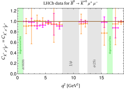
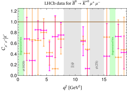
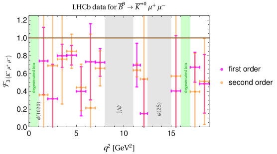
Figure 1: Results of $\mathcal{C}_{\bar{K}^{*}\mu^{+}|\mu^{-}}=\mathcal{C}_{\bar{K}^{*}\mu^{-}|\mu^{+}}$, $\mathcal{C}_{\mu^{-}\mu^{+}|\bar{K}^{*}}$ and $\mathcal{F}_{3(\bar{K}^{*}\mu^{-}\mu^{+})}$ for $\bar{B}^{0}\to\bar{K}^{*0}\mu^{+}\mu^{-}$ decay in each of the non-degenerated $q^{2}$ bins using LHCb data [75, 74]. The vertical error bars represent the $1\sigma$ uncertainty, where the first(second) order in the error propagation are shown in magenta(orange) colors. The horizontal bars correspond to the energy range of each bin. The gray shaded regions show the $\phi(1020)$, $J/\psi$ and $\psi(2S)$ resonances, which are vetoed. The green shaded regions represent the degenerated bins. The brown horizontal lines correspond to the maximal value of the quantifiers. The numerical values are collected in Tables LABEL:tab:results-LABEL:tab:resultsdegenerated of Appendix A

.

The results of the quantifiers $\mathcal{C}_{\bar{K}^{*}\mu^{+}|\mu^{-}}=\mathcal{C}_{\bar{K}^{*}\mu^{-}|\mu^{+}}$, $\mathcal{C}_{\mu^{-}\mu^{+}|\bar{K}^{*}}$ and $\mathcal{F}_{3(\bar{K}^{*}\mu^{-}\mu^{+})}$ associated to $\bar{B}^{0}\to\bar{K}^{*0}\mu^{+}\mu^{-}$ decay for each non-degenerated bins are shown in Fig. 1. The vertical error bars on this figure represent the 1$\sigma$ errors computed by propagating uncertainties across all input parameters at first (magenta) and second (orange) order. Horizontal bars represent the width of each energy bin. The corresponding values are gathered in Table LABEL:tab:results of Appendix A, in which the first and second lines correspond to the first and second order uncertainty propagation. Also in this appendix, the results for the degenerated bins corresponding to the green shaded regions are collected in Table LABEL:tab:resultsdegenerated. As a reference, the maximal quantifier value 1 is showed by the brown horizontal line in these plots. We expect similar results for the CP-conjugated $B^{0}\to K^{*0}\mu^{+}\mu^{-}$ decay since, in general, the CP-asymmetries are compatible with zero at 1$\sigma$ and the uncertainties at second order of $\mathcal{C}_{\mu^{-}\mu^{+}|K^{*}}$ and $\mathcal{F}_{3}$ cover the range $[0,1]$. For the same reason, we guess similar central values and size for the uncertainties of $K^{*0}$$\mu^{\pm}$ concurrences in both decays.

Using data at first order in error propagation, we found non-vanishing entanglement quantifiers for all non-degenerated bins by more than $1\sigma$, except for very particular cases. Therefore, we conclude that the three-body final states, and also the subsystems $K^{*0}$$\mu^{\pm}$ and $\mu^{-}\mu^{+}$, result entangled after the $B$ and $\bar{B}$ decays. These first order uncertainties are smaller for the $K^{*0}$$\mu^{\pm}$ concurrences in comparison to $\mathcal{C}_{\mu^{-}\mu^{+}|K^{*}}$ and $\mathcal{F}_{3(K^{*}\mu^{-}\mu^{+})}$, and the zero value is excluded with large significances (more than 5$\sigma$) for $\mathcal{C}_{\bar{K}^{*}\mu^{+}|\mu^{-}}=\mathcal{C}_{\bar{K}^{*}\mu^{-}|\mu^{+}}$. Furthermore, in some $q^{2}$ bins, values close to 1 of the quantifiers (compatible with maximally entangled states) are attained for less than 2$\sigma$ significance.

At second order in the error propagation, the previous picture changes since the resulting absolute uncertainties increase. The resulting central values are shifted according to Eq. (4.1) and they are compatible with the first order results at 1$\sigma$. The $K^{*0}$$\mu^{\pm}$ concurrences are still non-vanishing with large significance but, in general, $\mathcal{C}_{\mu^{-}\mu^{+}|K^{*}}$ and $\mathcal{F}_{3(K^{*}\mu^{-}\mu^{+})}$ almost cover the complete range $[0,1]$. Even more, some central values are greater than 1 now since the Taylor expansion breaks the expected range for the quantifiers. However, the associated uncertainties lead to results compatible with physical values. At the same line, some uncertainties get values above 1 at second order in the error propagation. In view of these results, the presence of entanglement in a system composed by one qutrit and two qubits is found in a collider environment for the first time.

The results for the degenerated energy bins are separately presented in Table LABEL:tab:resultsdegenerated. The particularity here is that the same data describe very different physical situations. For example, solution III in the $[16,17]$ bin is compatible with the complete range $[0,1]$ of the $K^{*0}$$\mu^{\pm}$ concurrences. However, solution II lies at more than 5$\sigma$($1\sigma$) from zero at first(second) order. A Similar situation is found for the others quantifiers using solutions I and II of $[0.1,0.98]$ bin.

Regarding the SM predictions for $\bar{B}^{0}\to\bar{K}^{*0}\mu^{+}\mu^{-}$ and as an illustrative example, we computed them with the FLAVIO package [98] in the low-$q^{2}$ regime, $[1.1,6]$ GeV², which involves the second to the sixth bin. We obtain the CP-averages and CP-asymmetries in Eq. (2.12) using the default parameters and form factors of this software (version 2.6.1). All bins result degenerated with these theoretical predictions. In addition, the associated theoretical uncertainties are smaller than the sensitivity reported by the LHCb collaboration and the second order error propagation is smoother for the second to fourth bins. The numerical values of each entanglement quantifier in the $1.1<q^{2}<6$ GeV² range are collected in Table LABEL:tab:resultsFlaviolow of Appendix A. The three theoretical solutions are compatible with data in Fig. 1 at 1$\sigma$ (except for the solution II of the $[3,4]$ GeV² bin for $\mathcal{C}_{\mu^{-}\mu^{+}|K^{*}}$ and $\mathcal{F}_{3(K^{*}\mu^{-}\mu^{+})}$ quantifiers at first order in the experimental uncertainties). Notice that the degeneracy would be resolved if the theoretical predictions of the helicity amplitudes were used instead of the CP-averages and CP-asymmetries but it appears they are not directly accessible from FLAVIO .

Finally, data was provided in energy bins of the invariant mass of the di-muon system. On the one hand, reliable theoretical predictions around the $\phi(1020)$, $J/\psi$ and $\psi(2S)$ resonances are not available. On the experimental side, the tree-level decays $B\to K^{*0}\phi$, $B\to K^{*0}J/\psi$ and $B\to K^{*0}\psi(2S)$ dominate the regions $0.98<q^{2}<1.1$ GeV², $8<q^{2}<11$ GeV² and $12.5<q^{2}<15$ GeV², respectively. They are the main source of backgrounds of this search [75, 74], hence these regions were removed from the experimental analysis. However, these two-body decays correspond to bipartite systems of two qutrits and the first two were analyzed in [52] (see also [55]). We close this section studying the post-decay and autodistillation phenomena [145, 146, 147, 29] which connect these bipartite systems, after the decay of the resonances into the $\mu^{+}\mu^{-}$ pair, with our tripartite final state. Concretely, we compute the amount of entanglement of the bipartite final state of $B\to K^{*}X$, for $X=\phi(1020)$, $J/\psi$ and $\psi(2S)$. The autodistillation phenomena occurs when the post-decay $X\to\mu^{+}\mu^{-}$ increases the entanglement between the muons and the $K^{*}$ meson, which is given by $\mathcal{C}_{K^{*}\mu^{+}|\mu^{-}}=\mathcal{C}_{K^{*}\mu^{-}|\mu^{+}}$, respect to the two-qutrit system $K^{*}X$.

Experimental data for the two-body decays correspond to the helicity amplitudes directly and they were reported in [148, 149, 150]. In particular, 4 observables determine the bipartite spin density matrix and this simplifies the analysis presented in our Section 2, in which we treat with 16 observables in order to reconstruct the 6 complex helicity amplitudes of the present three-body final state. In addition, we propagate the uncertainties of the entanglement quantifiers up to second order. The correlations in the uncertainties of the helicity amplitudes are not given by the experimental collaborations for $X=\phi(1020)$ and $\psi(2S)$, then we consider them as independent variables. In the previous studies [52, 55], the amount of entanglement was quantified via the entropy $\mathcal{E}$, defined in their Eq. (7), and the statistical analysis keeps just the first order. Now we compute the bipartite concurrences using data in order to perform a correspondence with the present analysis. If $\rho_{K^{*}X}$ denotes the spin density matrix of the (two-qutrit) $K^{*}X$-system after the $B\to K^{*}X$ decay, the resulting bipartite concurrence for this pure state was defined in [151] as

$$\mathcal{C}_{2}[\rho_{K^{*}X}]=\sqrt{2(1-{\rm Tr}[(\rho_{K^{*}})^{2}])}=\sqrt{2(1-{\rm Tr}[(\rho_{X})^{2}])}$$ (4.3)

where $\rho_{K^{*}}$ and $\rho_{X}$ are the reduced matrices tracing over $K^{*}$ and $X$, respectively. The same holds for the CP-conjugated decay $\bar{B}\to\bar{K}^{*}X$. The spin density matrix in terms of the transversity amplitudes for these bipartite states were reported in Eqs. (5)-(6) of [52], from which we find

$$\mathcal{C}_{2}[\rho_{K^{*}X}]=\sqrt{2-2|\mathcal{A}_{0}|^{4}-|\mathcal{A}_{\perp}|^{4}-|\mathcal{A}_{\parallel}|^{4}-4|\mathcal{A}_{\perp}|^{2}|\mathcal{A}_{\parallel}|^{2}-2|\mathcal{A}_{\perp}|^{2}|\mathcal{A}_{\parallel}|^{2}\cos 2(\phi_{\perp}-\phi_{\parallel})}$$ (4.4)

Combining data from both channels, the results for the entanglement quantifiers up to second order in the error propagation are collected in Table LABEL:tab:resultsFabbrichesi.

Table 1: Values of entropy of entanglement $\mathcal{E}$ and bipartite concurrence $\mathcal{C}_{2}$ corresponding to both $B\to K^{*}X$ and $\bar{B}\to\bar{K}^{*}X$ decays for each resonance $X=\phi(1020)$, $J/\psi$ and $\psi(2S)$. First(second) line in the last two columns corresponds to the first(second) order error propagation.

$B\to K^{*}X$ decays	$m_{X}^{2}$ [GeV2]	$\mathcal{E}$	$\mathcal{C}_{2}$
$B\to K^{*}\phi$	$1.038$	$0.707\pm 0.133$	$0.998\pm 0.025$
		$0.769\pm 0.119$	$0.998\pm 0.047$
$B\to K^{*}J/\psi$	$9.591$	$0.756\pm 0.009$	$1.004\pm 0.004$
		$0.756\pm 0.009$	$1.004\pm 0.004$
$B\to K^{*}\psi(2S)$	$13.587$	$0.880\pm 0.172$	$0.760\pm 0.059$
		$0.858\pm 0.178$	$1.23\pm 0.21$

We recover the previous results [52] for the entropy of entanglement and conclude with large significance, also from the bipartite concurrence, that these two-qutrit systems result entangled, i.e. they are non-separable. Including second order corrections in the error propagation, these results are stable (in particular for the $J/\psi$ resonance). We understand this behaviour from the smoothness of the concurrences with respect to the helicity amplitude data in Eq. (4.4).

Notice that $\mathcal{C}_{2}$ has a theoretical maximum equals to $\sqrt{4/3}$ and data is beyond 5$\sigma$ from that value, except for the second order in the $\psi(2S)$ resonance. Even though we do not have data corresponding to the three-body decays $B\to K^{*}X(\to\mu^{+}\mu^{-})$ in the gray shaded regions of Fig. 1, we can compare with respect to $K^{*0}$$\mu^{\pm}$ concurrences in the adjacent non-degenerated energy bins: $[1.1,2]$ for $\phi(1020)$, $[7,8]$-$[11,11.75]$ for $J/\psi$, and $[11.75,12.5]$-$[15,16]$ for $\psi(2S)$. In all cases, the corresponding maximum is within 1$\sigma$ which might lead to expect a possible autodistillation phenomenon in these $B$ meson decays.

5 Conclusions

In this work, we develop a spin quantum tomography program for a tripartite system composed by one qutrit and two qubits, which arises in the three-body decay of a spin 0 state ($S$) into one massive vector ($V$) and two fermion particles ($f^{+}f^{-}$ pair). Concretely, we focus on semi-leptonic $B$ meson decays via the one-loop $b\to ql^{+}l^{-}$ transitions which have received significant attention in recent years from both experimental and theoretical sides due to observed deviations from SM in some angular and lepton flavor universality observables and also to the opportunity to search NP in this kind of processes. Here, we provide a novel application of entanglement observables in order to test the quantum mechanical nature of the strong and electroweak interactions in collider physics.

Our analysis is based on the reconstruction, provided by dedicated experimental searches, of the helicity amplitudes and the spin density matrix that describes the final state polarizations. With this information, different entanglement quantifiers associated to the tripartite system are computed, including the uncertainty and correlations of the measurements at second order in the error propagation, in order to determine the corresponding significances. Multipartite entanglement has a more complex structure than the bipartite case, then we computed the one-to-other concurrences associated to the vector-fermion and di-fermion subsystems with the aim to establish the partial biseparability of the final state. In addition, the amount of genuine entanglement is calculated by the area of the concurrence triangle. Assuming massless fermions and the absence of scalar and pseudoscalar operators, the $S\to Vf^{+}f^{-}$ decays have 6 non-vanishing complex helicity amplitudes and are fully described by the di-fermion invariant mass squared ($q^{2}$) and three angles between the decay products. In particular, 12 angular coefficients determine the differential partial width and they are related to the experimental CP-averages and CP-asymmetries observables. To recover the helicity amplitudes from these measurements is a non-trivial task and the entanglement quantifiers are given in terms of $q^{2}$. With the available data, ambiguities arise in some cases resulting in different entanglement predictions.

As an application of our analysis, using data recorded by the LHCb experiment corresponding to $B^{0}\to K^{*0}\mu^{+}\mu^{-}$ decays in the energy range $0.1<q^{2}<19$ GeV², we performed a complete quantum tomography of this tripartite system. At first order in the error propagation, we found the presence of genuine quantum entanglement in the final state, and also in the di-muon subsystem by more than 1$\sigma$ in most of the energy bins. For the $K^{*0}$$\mu^{\pm}$ subsystem, the resulting uncertainties are smaller than in the other two quantifiers and non-vanishing concurrences are attained with more than 5$\sigma$ and the maximal entanglement value is reached within 1$\sigma$ in most of the energy bins. In order to control the propagation of uncertainties, we performed a second order expansion where, in general, the central values of the quantifiers change and the uncertainties increase. The results at first and second order are compatible at 1$\sigma$ and the presence of entanglement is established in $\mathcal{C}_{\bar{K}^{*}\mu^{-}|\mu^{+}}=\mathcal{C}_{\bar{K}^{*}\mu^{+}|\mu^{-}}$ and in certain energy bins of the other quantifiers. Contact with previous works in bipartite $B$ meson decays was also provided in the energy range corresponding to the $\phi(1020)$, $J/\psi$ and $\psi(2S)$ resonances by studying the post-decay and autodistillation phenomena.

As far as we know, these three-body decays are the only ones with full dedicated experimental data corresponding to angular distributions of the final particles. The present analysis can be straightforwardly applied to many other processes if the lacking experimental information on CP-averages and CP-asymmetries for the helicity amplitudes reconstruction were available. There is much more information in the complete set of angular coefficients than in the differential branching ratios, some particular angular observables or lepton flavor universality tests. The proposed quantifiers from angular distributions provide new perspectives to study fundamental interactions at colliders.

Regarding the SM predictions, the theoretical computations have limited precision mainly due to the non-local contributions of charmonium resonances. However, the entanglement quantifiers measurements might also provide information about the Wilson coefficients and constraint the presence of NP in this kind of transitions. This also represents possible future avenues to be explored in this context.

Data Availability Statement

There is no associated data generated during this work.

Code Availability Statement

Code/Software sharing not applicable to this article as no code/software was generated or analysed during the current study.

Appendices

Appendix A Tables of results

The numerical values of the entanglement quantifiers showed in Fig. 1 are collected in Table LABEL:tab:results. The first and second lines correspond to the first and second order uncertainty propagation.

Table 2: Values of $\mathcal{C}_{\bar{K}^{*}\mu^{+}|\mu^{-}}=\mathcal{C}_{\bar{K}^{*}\mu^{-}|\mu^{+}}$, $\mathcal{C}_{\mu^{-}\mu^{+}|\bar{K}^{*}}$ and $\mathcal{F}_{3(\bar{K}^{*}\mu^{-}\mu^{+})}$ corresponding to $\bar{B}^{0}\to\bar{K}^{*0}\mu^{+}\mu^{-}$ decay for each non-degenerated bins using LHCb data [75, 74]. First(second) line in last three columns corresponds to first(second) order error propagation.

Energy bin [GeV2]	$\mathcal{C}_{\bar{K}^{*}\mu^{+}|\mu^{-}}=\mathcal{C}_{\bar{K}^{*}\mu^{-}|\mu^{+}}$	$\mathcal{C}_{\mu^{-}\mu^{+}|\bar{K}^{*}}$	$\mathcal{F}_{3(\bar{K}^{*}\mu^{-}\mu^{+})}$
$[1.1,2]$	$0.9999\pm 0.0058$	$0.68\pm 0.40$	$0.74\pm 0.38$
	$0.91\pm 0.14$	$0.41\pm 1.39$	$0.36\pm 6.91$
$[2,3]$	$0.986\pm 0.075$	$0.28\pm 0.36$	$0.32\pm 0.39$
	$0.92\pm 0.35$	$0.67\pm 2.53$	$0.69\pm 2.66$
$[3,4]$	$0.917\pm 0.058$	$0.85\pm 0.17$	$0.80\pm 0.13$
	$1.01\pm 0.11$	$0.66\pm 0.64$	$0.76\pm 0.50$
$[4,5]$	$0.929\pm 0.043$	$0.84\pm 0.15$	$0.81\pm 0.11$
	$1.005\pm 0.064$	$0.80\pm 0.26$	$0.85\pm 0.19$
$[5,6]$	$0.982\pm 0.037$	$0.36\pm 0.27$	$0.40\pm 0.28$
	$0.964\pm 0.014$	$0.43\pm 0.23$	$0.44\pm 0.26$
$[6,7]$	$0.95\pm 0.21$	$0.72\pm 0.39$	$0.73\pm 0.43$
	$0.95\pm 0.35$	$0.13\pm 0.96$	$0.21\pm 0.83$
$[7,8]$	$0.913\pm 0.059$	$0.76\pm 0.23$	$0.73\pm 0.16$
	$0.940\pm 0.046$	$0.68\pm 0.28$	$0.66\pm 0.20$
$[11,11.75]$	$0.994\pm 0.037$	$0.64\pm 0.27$	$0.70\pm 0.25$
	$0.95\pm 0.19$	$0.654\pm 0.079$	$0.638\pm 0.075$
$[11.75,12.5]$	$0.996\pm 0.023$	$0.13\pm 0.34$	$0.15\pm 0.39$
	$0.959\pm 0.065$	$0.49\pm 1.11$	$0.54\pm 1.21$
$[15,16]$	$0.99\pm 0.10$	$0.36\pm 0.61$	$0.40\pm 0.62$
	$0.78\pm 0.23$	$0.72\pm 1.06$	$0.57\pm 1.15$
$[17,18]$	$0.88\pm 0.19$	$0.73\pm 0.23$	$0.67\pm 0.17$
	$0.95\pm 0.40$	$0.34\pm 0.70$	$0.40\pm 0.43$
$[18,19]$	$0.9992\pm 0.0070$	$0.43\pm 0.31$	$0.48\pm 0.33$
	$0.983\pm 0.037$	$0.48\pm 0.61$	$0.51\pm 0.48$

Furthermore, the results for the degenerated bins are gathered in Table LABEL:tab:resultsdegenerated. In this case, each bin has three solutions for the 12 angular coefficients compatible with data.

Table 3: Values of $\mathcal{C}_{\bar{K}^{*}\mu^{+}|\mu^{-}}=\mathcal{C}_{\bar{K}^{*}\mu^{-}|\mu^{+}}$, $\mathcal{C}_{\mu^{-}\mu^{+}|\bar{K}^{*}}$ and $\mathcal{F}_{3(\bar{K}^{*}\mu^{-}\mu^{+})}$ corresponding to $\bar{B}^{0}\to\bar{K}^{*0}\mu^{+}\mu^{-}$ decay for each solution of the degenerated bins using LHCb data [75, 74]. First(second) line in last three columns corresponds to first(second) order error propagation.

Energy bin [GeV2]	$\mathcal{C}_{\bar{K}^{*}\mu^{+}|\mu^{-}}=\mathcal{C}_{\bar{K}^{*}\mu^{-}|\mu^{+}}$	$\mathcal{C}_{\mu^{-}\mu^{+}|\bar{K}^{*}}$	$\mathcal{F}_{3(\bar{K}^{*}\mu^{-}\mu^{+})}$
$[0.1,0.98]$ solution I	$0.996\pm 0.018$	$0.977\pm 0.043$	$0.979\pm 0.048$
	$0.966\pm 0.025$	$0.882\pm 0.050$	$0.876\pm 0.049$
$[0.1,0.98]$ solution II	$0.89\pm 0.25$	$0.45\pm 0.61$	$0.45\pm 0.45$
	$1.28\pm 0.76$	$0.75\pm 1.68$	$0.68\pm 1.64$
$[0.1,0.98]$ solution III	$0.918\pm 0.098$	$0.79\pm 0.24$	$0.76\pm 0.24$
	$1.30\pm 0.32$	$0.91\pm 0.33$	$1.23\pm 0.46$
$[16,17]$ solution I	$0.66\pm 0.48$	$0.56\pm 0.22$	$0.39\pm 0.44$
	$0.27\pm 0.57$	$0.47\pm 0.80$	$0.13\pm 0.48$
$[16,17]$ solution II	$0.96\pm 0.16$	$0.48\pm 0.53$	$0.52\pm 0.44$
	$0.60\pm 0.52$	$0.82\pm 0.85$	$0.49\pm 0.50$
$[16,17]$ solution III	$0.70\pm 0.82$	$0.60\pm 0.31$	$0.44\pm 0.78$
	$0.64\pm 1.09$	$0.18\pm 4.56$	$0.16\pm 1.27$

Finally, we collect the numerical values of the SM predictions derived with FLAVIO package in Table LABEL:tab:resultsFlaviolow. They correspond to five bins in the energy range $1.1<q^{2}<6$ GeV² and were obtained with default values of parameters and form factors of version 2.6.1. This theoretical computation predicts three solutions for each bin.

Table 4: SM predictions for $\mathcal{C}_{\bar{K}^{*}\mu^{+}|\mu^{-}}=\mathcal{C}_{\bar{K}^{*}\mu^{-}|\mu^{+}}$, $\mathcal{C}_{\mu^{-}\mu^{+}|\bar{K}^{*}}$ and $\mathcal{F}_{3(\bar{K}^{*}\mu^{-}\mu^{+})}$ corresponding to $\bar{B}^{0}\to\bar{K}^{*0}\mu^{+}\mu^{-}$ decay in the range $1.1<q^{2}<6$ GeV² using FLAVIO package (version 2.6.1) with default parameters and form factors. The three solutions of each bin are shown. First(second) line in the last three columns corresponds to the first(second) order error propagation.

Energy bin [GeV2]	$\mathcal{C}_{\bar{K}^{*}\mu^{+}|\mu^{-}}=\mathcal{C}_{\bar{K}^{*}\mu^{-}|\mu^{+}}$	$\mathcal{C}_{\mu^{-}\mu^{+}|\bar{K}^{*}}$	$\mathcal{F}_{3(\bar{K}^{*}\mu^{-}\mu^{+})}$
$[1.1,2]$ solution I	$0.99975\pm 0.00030$	$0.9785\pm 0.0021$	$0.9851\pm 0.0015$
	$0.99961\pm 0.00033$	$0.9782\pm 0.0028$	$0.9847\pm 0.0020$
$[1.1,2]$ solution II	$0.710\pm 0.036$	$0.705\pm 0.037$	$0.502\pm 0.051$
	$0.716\pm 0.038$	$0.695\pm 0.038$	$0.504\pm 0.052$
$[1.1,2]$ solution III	$0.815\pm 0.019$	$0.807\pm 0.024$	$0.659\pm 0.030$
	$0.813\pm 0.031$	$0.773\pm 0.057$	$0.640\pm 0.058$
$[2,3]$ solution I	$0.9988\pm 0.0016$	$0.9864\pm 0.0013$	$0.9893\pm 0.0019$
	$0.9983\pm 0.0017$	$0.9865\pm 0.0016$	$0.9887\pm 0.0020$
$[2,3]$ solution II	$0.863\pm 0.058$	$0.38\pm 0.13$	$0.373\pm 0.093$
	$0.876\pm 0.061$	$0.37\pm 0.13$	$0.352\pm 0.097$
$[2,3]$ solution III	$0.951\pm 0.054$	$0.490\pm 0.053$	$0.520\pm 0.026$
	$0.948\pm 0.059$	$0.500\pm 0.060$	$0.524\pm 0.040$
$[3,4]$ solution I	$0.995\pm 0.0097$	$0.9790\pm 0.0054$	$0.980\pm 0.016$
	$0.990\pm 0.012$	$0.969\pm 0.010$	$0.966\pm 0.021$
$[3,4]$ solution II	$0.981\pm 0.057$	$0.10\pm 0.12$	$0.12\pm 0.13$
	$0.93\pm 0.10$	$0.09\pm 0.13$	$0.08\pm$0.14
$[3,4]$ solution III	$0.967\pm 0.067$	$0.576\pm 0.083$	$0.61\pm 0.11$
	$0.914\pm 0.091$	$0.555\pm 0.097$	$0.56\pm 0.14$
$[4,5]$ solution I	$0.976\pm 0.044$	$0.952\pm 0.032$	$0.937\pm 0.077$
	$0.948\pm 0.057$	$0.920\pm 0.047$	$0.88\pm 0.10$
$[4,5]$ solution II	$0.71\pm 0.37$	$0.246\pm 0.083$	$0.20\pm 0.14$
	$0.57\pm 0.54$	$0.17\pm 0.20$	$0.11\pm 0.26$
$[4,5]$ solution III	$0.80\pm 0.33$	$0.64\pm 0.22$	$0.54\pm 0.42$
	$0.56\pm 0.49$	$0.54\pm 0.29$	$0.36\pm 0.55$
$[5,6]$ solution I	$0.90\pm 0.25$	$0.87\pm 0.19$	$0.79\pm 0.40$
	$0.56\pm 0.47$	$0.50\pm 0.48$	$0.22\pm 0.79$
$[5,6]$ solution II	$0.39\pm 0.76$	$0.18\pm 0.32$	$0.08\pm 0.28$
	$0.51\pm 1.85$	$0.28\pm 0.90$	$0.36\pm 0.52$
$[5,6]$ solution III	$0.61\pm 1.11$	$0.54\pm 0.83$	$0.34\pm 1.17$
	$0.33\pm 2.10$	$0.09\pm 1.55$	$0.37\pm 2.01$

Appendix B Statistical analysis

Consider a set of variables $y_{\lambda}$ which are functions of $n$ input variables $x_{i}$: $y_{\lambda}=f_{\lambda}(\vec{x})=f_{\lambda}(x_{1},...,x_{n})$. The derivation of the resulting error propagation comes from a Taylor series expansion, then it is valid locally around the central (mean) input values $\langle\vec{x}\rangle=E[\vec{x}]$ and this approximation is generically more accurate for polynomial-type functions $f$. The second-order Taylor expansion around the input means is

$$y_{\lambda}\approx f_{\lambda}(\langle\vec{x}\rangle)+\sum_{i}\frac{\partial f_{\lambda}}{\partial x_{i}}(x_{i}-\langle x_{i}\rangle)+\frac{1}{2}\sum_{i,j}\frac{\partial^{2}f_{\lambda}}{\partial x_{i}\partial x_{j}}(x_{i}-\langle x_{i}\rangle)(x_{j}-\langle x_{j}\rangle)$$ (B.1)

The central (expectation) value at second order in the multivariable case is

$$\langle y_{\lambda}\rangle=E[y_{\lambda}]=f_{\lambda}(\langle\vec{x}\rangle)+\frac{1}{2}\sum_{i,j}\frac{\partial^{2}f_{\lambda}}{\partial x_{i}\partial x_{j}}\sigma_{ij}^{2}$$ (B.2)

where we assumed symmetric uncertainties for the input variables, we used $E[x_{i}-\langle x_{i}\rangle]=0$ and we introduced the covariance of the inputs as $\sigma_{ij}^{2}=E[(x_{i}-\langle x_{i}\rangle)(x_{j}-\langle x_{j}\rangle)]$. In a similar way, the covariance of $y$ variables is defined as $\sigma_{\lambda\eta}^{2}=E[(y_{\lambda}-\langle y_{\lambda}\rangle)(y_{\eta}-\langle y_{\eta}\rangle)]$. In particle physics, it is usually considered just the first order in the error propagation. Combining the previous equations, we arrive to the well known expression [152]

$$\sigma_{\lambda\eta}^{2}|_{\text{$1^{st}$ order}}=\sum_{i,j}\frac{\partial f_{\lambda}}{\partial x_{i}}\frac{\partial f_{\eta}}{\partial x_{j}}\sigma_{ij}^{2}$$ (B.3)

The second order involves several terms. The main assumption to treat them is that the $\vec{x}$ and $y$ variables are considered as Gaussian, then they are described by just the mean and variance. In particular, non-Gaussian terms, such as skewness and kurtosis, are neglected. The non-vanishing corrections at second order in the error propagation are given by

$$\sigma_{\lambda\eta}^{2}|_{\text{$2^{nd}$ order}} = \frac{1}{4}\sum_{i}\frac{\partial^{2}f_{\lambda}}{\partial x_{i}^{2}}\frac{\partial^{2}f_{\eta}}{\partial x_{i}^{2}}\mu_{4}^{i}+\frac{1}{4}\sum_{i\neq j}\left(\frac{\partial^{2}f_{\lambda}}{\partial x_{i}\partial x_{j}}\frac{\partial^{2}f_{\eta}}{\partial x_{i}^{2}}+\frac{\partial^{2}f_{\lambda}}{\partial x_{i}^{2}}\frac{\partial^{2}f_{\eta}}{\partial x_{i}\partial x_{j}}\right)2\mu_{3,1}^{i,j}$$ (B.4)

$$+\frac{1}{4}\sum_{i\neq j}\left(\frac{\partial^{2}f_{\lambda}}{\partial x_{i}\partial x_{j}}\frac{\partial^{2}f_{\eta}}{\partial x_{i}\partial x_{j}}2+\frac{\partial^{2}f_{\lambda}}{\partial x_{i}^{2}}\frac{\partial^{2}f_{\eta}}{\partial x_{j}^{2}}\right)\mu_{2,2}^{i,j}$$

$$+\frac{1}{4}\sum_{i\neq i^{\prime}\neq j^{\prime}}\left(\frac{\partial^{2}f_{\lambda}}{\partial x_{i}^{2}}\frac{\partial^{2}f_{\eta}}{\partial x_{i^{\prime}}\partial x_{j^{\prime}}}+\frac{\partial^{2}f_{\lambda}}{\partial x_{i^{\prime}}\partial x_{j^{\prime}}}\frac{\partial^{2}f_{\eta}}{\partial x_{i}^{2}}\right)\mu_{2,1,1}^{i,i^{\prime},j^{\prime}}$$

$$+\frac{1}{4}\sum_{i\neq j\neq j^{\prime}}\frac{\partial^{2}f_{\lambda}}{\partial x_{i}\partial x_{j}}\frac{\partial^{2}f_{\eta}}{\partial x_{i}\partial x_{j^{\prime}}}4\mu_{2,1,1}^{i,j,j^{\prime}}+\frac{1}{4}\sum_{i\neq j\neq i^{\prime}\neq j^{\prime}}\frac{\partial^{2}f_{\lambda}}{\partial x_{i}\partial x_{j}}\frac{\partial^{2}f_{\eta}}{\partial x_{i^{\prime}}\partial x_{j^{\prime}}}4\mu_{1,1,1,1}^{i,j,i^{\prime},j^{\prime}}$$

$$-\frac{1}{4}\sum_{i,j,i^{\prime},j^{\prime}}\frac{\partial^{2}f_{\lambda}}{\partial x_{i}\partial x_{j}}\frac{\partial^{2}f_{\eta}}{\partial x_{i^{\prime}}\partial x_{j^{\prime}}}\sigma_{ij}^{2}\sigma_{i^{\prime}j^{\prime}}^{2}$$

For compactness in the previous equation, introduced the central moments of order ${p_{1},\ldots,p_{m}}$ as

$$\mu_{p_{1},\ldots,p_{m}}^{i_{1},\ldots,i_{m}}=\int_{-\infty}^{\infty}(x_{i_{1}}-\langle x_{i_{1}}\rangle)^{p_{1}}\ldots(x_{i_{m}}-\langle x_{i_{m}}\rangle)^{p_{m}}\mathcal{G}(x_{i_{1}},\ldots,x_{i_{m}})dx_{i_{1}}\ldots dx_{i_{m}}$$ (B.5)

where $\mathcal{G}$ is the Gaussian distribution function of the input variables. We computed the relevant central moments for correlated variables by diagonalizing their correlation matrix $\sigma^{2}$ and taking into account that the independent $\vec{x}$ variable case can be computed as one-dimensional Gaussian integrals. We arrive to the following expressions

$$\mu_{4}^{i}=3\sigma_{ii}^{4}\,,\quad\mu_{3,1}^{i,j}=3\sigma_{ii}^{2}\sigma_{ij}^{2}\,,$$

$$\mu_{2,2}^{i,j}=2\sigma_{ij}^{4}+\sigma_{ii}^{2}\sigma_{jj}^{2}\,,\quad\mu_{2,1,1}^{i,j,j^{\prime}}=2\sigma_{ij}^{2}\sigma_{ij^{\prime}}^{2}+\sigma_{ii}^{2}\sigma_{jj^{\prime}}^{2}\,,$$

$$\mu_{1,1,1,1}^{i,j,i^{\prime},j^{\prime}}=\sigma_{ij}^{2}\sigma_{i^{\prime}j^{\prime}}^{2}+\sigma_{ii^{\prime}}^{2}\sigma_{jj^{\prime}}^{2}+\sigma_{ij^{\prime}}^{2}\sigma_{ji^{\prime}}^{2}\,,$$

$$\mu_{p_{1},\ldots,p_{m}}^{i_{1},\ldots,i_{m}}=0\,\,(\text{if $p_{1}+\ldots+p_{m}$ is odd})$$ (B.6)

Notice that the uncorrelated input case simplifies the computation since the central moments vanish if some $p_{i}$ is odd, and just $\mu_{4}^{k}=3\sigma_{kk}^{4}$ and $\mu_{2,2}^{k,k^{\prime}}=\sigma_{kk}^{2}\sigma_{k^{\prime}k^{\prime}}^{2}$ survive.

Inserting Eq. (B.6) into Eq. (B.4) and after tedious algebra, we conclude that the correlation between the $y$ variables up to second order is

$$E[(y_{\lambda}-\langle y_{\lambda}\rangle)(y_{\eta}-\langle y_{\eta}\rangle)]=\sum_{i,j}\frac{\partial f_{\lambda}}{\partial x_{i}}\frac{\partial f_{\eta}}{\partial x_{j}}\sigma_{ij}^{2}+\frac{1}{4}\sum_{i,j,i^{\prime},j^{\prime}}\frac{\partial^{2}f_{\lambda}}{\partial x_{i}\partial x_{j}}\frac{\partial^{2}f_{\eta}}{\partial x_{i^{\prime}}\partial x_{j^{\prime}}}\left(\sigma_{ii^{\prime}}^{2}\sigma_{jj^{\prime}}^{2}+\sigma_{ij^{\prime}}^{2}\sigma_{ji^{\prime}}^{2}\right)$$ (B.7)

This expression is in agreement with the uncorrelated input variables case [153, 154] and reduces to the one-variable case in Eq. (4.2), which is the relevant one for our work. In particular, the partial derivatives of the entanglement quantifiers respect to the CP-averages and CP-asymmetries (input variables) were computed using the chain rule (via the helicity amplitudes) due to the complexity of the corresponding expressions. At first order, this error propagation procedure just introduces the correlation matrix of the helicity amplitudes [152]

$$\sigma_{\mathcal{C}(\mathcal{O})}^{2} = \sum_{i,j}\frac{\partial\mathcal{C}}{\partial x_{i}}\frac{\partial\mathcal{C}}{\partial x_{j}}\sigma_{ij}^{2}=\sum_{i,j}\left(\sum_{\lambda}\frac{\partial\mathcal{C}}{\partial\mathcal{A}_{\lambda}}\frac{\partial\mathcal{A}_{\lambda}}{\partial x_{i}}\right)\left(\sum_{\eta}\frac{\partial\mathcal{C}}{\partial\mathcal{A}_{\eta}}\frac{\partial\mathcal{A}_{\eta}}{\partial x_{j}}\right)\sigma_{ij}^{2}$$ (B.8)

$$= \sum_{\lambda,\eta}\frac{\partial\mathcal{C}}{\partial\mathcal{A}_{\lambda}}\frac{\partial\mathcal{C}}{\partial\mathcal{A}_{\eta}}\left(\sum_{i,j}\frac{\partial\mathcal{A}_{\lambda}}{\partial x_{i}}\frac{\partial\mathcal{A}_{\eta}}{\partial x_{j}}\sigma_{ij}^{2}\right)=\sum_{\lambda,\eta}\frac{\partial\mathcal{C}}{\partial\mathcal{A}_{\lambda}}\frac{\partial\mathcal{C}}{\partial\mathcal{A}_{\eta}}\sigma_{\mathcal{A}_{\lambda}\mathcal{A}_{\eta}}^{2}=\sigma_{\mathcal{C}(\mathcal{A}(\mathcal{O}))}^{2}$$

However, the chain rule for the second order partial derivatives

$$\frac{\partial^{2}\mathcal{C}}{\partial x_{i}\partial x_{j}}=\sum_{\lambda,\eta}\frac{\partial^{2}\mathcal{C}}{\partial\mathcal{A}_{\lambda}\partial\mathcal{A}_{\eta}}\frac{\partial\mathcal{A}_{\lambda}}{\partial x_{i}}\frac{\partial\mathcal{A}_{\eta}}{\partial x_{j}}+\sum_{\lambda}\frac{\partial\mathcal{C}}{\partial\mathcal{A}_{\lambda}}\frac{\partial^{2}\mathcal{A}_{\lambda}}{\partial x_{i}\partial x_{j}}$$ (B.9)

introduces additional terms that can not be identified with the correlation matrix of the helicity amplitudes at second order. We keep all of them for the present analysis.

References

- [1] J. S. Bell, On the einstein podolsky rosen paradox, Physics Physique Fizika 1 (1964) 195.
- [2] R. Horodecki, P. Horodecki, M. Horodecki and K. Horodecki, Quantum entanglement, Rev. Mod. Phys. 81 (2009) 865 [quant-ph/0702225].
- [3] N. Brunner, D. Cavalcanti, S. Pironio, V. Scarani and S. Wehner, Bell nonlocality, Rev. Mod. Phys. 86 (2014) 419 [1303.2849].
- [4] A. K. Ekert, Quantum cryptography based on bell’s theorem, Phys. Rev. Lett. 67 (1991) 661.
- [5] C. H. Bennett, G. Brassard, C. Crépeau, R. Jozsa, A. Peres and W. K. Wootters, Teleporting an unknown quantum state via dual classical and einstein-podolsky-rosen channels, Phys. Rev. Lett. 70 (1993) 1895.
- [6] R. Raussendorf and H. J. Briegel, A one-way quantum computer, Phys. Rev. Lett. 86 (2001) 5188.
- [7] A. Aspect, P. Grangier and G. Roger, Experimental realization of einstein-podolsky-rosen-bohm gedankenexperiment: A new violation of bell’s inequalities, Phys. Rev. Lett. 49 (1982) 91.
- [8] E. Hagley, X. Maître, G. Nogues, C. Wunderlich, M. Brune, J. M. Raimond et al., Generation of einstein-podolsky-rosen pairs of atoms, Phys. Rev. Lett. 79 (1997) 1.
- [9] M. Steffen, M. Ansmann, R. C. Bialczak, N. Katz, E. Lucero, R. McDermott et al., Measurement of the entanglement of two superconducting qubits via state tomography, Science 313 (2006) 1423 [https://www.science.org/doi/pdf/10.1126/science.1130886].
- [10] W. Pfaff, T. H. Taminiau, L. Robledo, H. Bernien, M. Markham, D. J. Twitchen et al., Demonstration of entanglement-by-measurement of solid-state qubits, Nature Phys. 9 (2012) 29.
- [11] B. Julsgaard, A. Kozhekin and E. S. Polzik, Experimental long-lived entanglement of two macroscopic objects, Nature 413 (2001) 400.
- [12] C. F. Ockeloen-Korppi, E. Damskägg, J. M. Pirkkalainen, A. A. Clerk, F. Massel, M. J. Woolley et al., Stabilized entanglement of massive mechanical oscillators, Nature 556 (2018) 478 [1711.01640].
- [13] S. Storz et al., Loophole-free Bell inequality violation with superconducting circuits, Nature 617 (2023) 265.
- [14] A. J. Barr, M. Fabbrichesi, R. Floreanini, E. Gabrielli and L. Marzola, Quantum entanglement and Bell inequality violation at colliders, 2402.07972.
- [15] ATLAS collaboration, Observation of quantum entanglement in top-quark pairs using the ATLAS detector, 2311.07288.
- [16] CMS collaboration, Observation of quantum entanglement in top quark pair production in proton-proton collisions at = 13 TeV, 2406.03976.
- [17] CMS collaboration, Measurements of polarization and spin correlation and observation of entanglement in top quark pairs using lepton+jets events from proton-proton collisions at = 13 TeV, 2409.11067.
- [18] Y. Afik and J. R. M. n. de Nova, Entanglement and quantum tomography with top quarks at the LHC, Eur. Phys. J. Plus 136 (2021) 907 [2003.02280].
- [19] Y. Afik and J. R. M. n. de Nova, Quantum information with top quarks in QCD, Quantum 6 (2022) 820 [2203.05582].
- [20] M. Fabbrichesi, R. Floreanini and G. Panizzo, Testing Bell Inequalities at the LHC with Top-Quark Pairs, Phys. Rev. Lett. 127 (2021) 161801 [2102.11883].
- [21] C. Severi, C. D. E. Boschi, F. Maltoni and M. Sioli, Quantum tops at the LHC: from entanglement to Bell inequalities, Eur. Phys. J. C 82 (2022) 285 [2110.10112].
- [22] J. A. Aguilar-Saavedra and J. A. Casas, Improved tests of entanglement and Bell inequalities with LHC tops, Eur. Phys. J. C 82 (2022) 666 [2205.00542].
- [23] Y. Afik and J. R. M. n. de Nova, Quantum Discord and Steering in Top Quarks at the LHC, Phys. Rev. Lett. 130 (2023) 221801 [2209.03969].
- [24] Z. Dong, D. Gonçalves, K. Kong and A. Navarro, When the Machine Chimes the Bell: Entanglement and Bell Inequalities with Boosted , 2305.07075.
- [25] T. Han, M. Low and T. A. Wu, Quantum entanglement and Bell inequality violation in semi-leptonic top decays, JHEP 07 (2024) 192 [2310.17696].
- [26] M. Fabbrichesi, R. Floreanini and E. Gabrielli, Constraining new physics in entangled two-qubit systems: top-quark, tau-lepton and photon pairs, Eur. Phys. J. C 83 (2023) 162 [2208.11723].
- [27] M. M. Altakach, P. Lamba, F. Maltoni, K. Mawatari and K. Sakurai, Quantum information and CP measurement in H→+- at future lepton colliders, Phys. Rev. D 107 (2023) 093002 [2211.10513].
- [28] K. Ma and T. Li, Testing Bell inequality through at CEPC, 2309.08103.
- [29] R. A. Morales, Tripartite entanglement and Bell non-locality in loop-induced Higgs boson decays, Eur. Phys. J. C 84 (2024) 581 [2403.18023].
- [30] A. J. Barr, Testing Bell inequalities in Higgs boson decays, Phys. Lett. B 825 (2022) 136866 [2106.01377].
- [31] J. A. Aguilar-Saavedra, Laboratory-frame tests of quantum entanglement in H→WW, Phys. Rev. D 107 (2023) 076016 [2209.14033].
- [32] J. A. Aguilar-Saavedra, A. Bernal, J. A. Casas and J. M. Moreno, Testing entanglement and Bell inequalities in H→ZZ, Phys. Rev. D 107 (2023) 016012 [2209.13441].
- [33] R. Ashby-Pickering, A. J. Barr and A. Wierzchucka, Quantum state tomography, entanglement detection and Bell violation prospects in weak decays of massive particles, JHEP 05 (2023) 020 [2209.13990].
- [34] M. Fabbrichesi, R. Floreanini, E. Gabrielli and L. Marzola, Bell inequalities and quantum entanglement in weak gauge boson production at the LHC and future colliders, Eur. Phys. J. C 83 (2023) 823 [2302.00683].
- [35] A. Bernal, P. Caban and J. Rembieliński, Entanglement and Bell inequalities violation in with anomalous coupling, Eur. Phys. J. C 83 (2023) 1050 [2307.13496].
- [36] F. Fabbri, J. Howarth and T. Maurin, Isolating semi-leptonic decays for Bell inequality tests, Eur. Phys. J. C 84 (2024) 20 [2307.13783].
- [37] Y. Afik, Y. Kats, J. R. M. n. de Nova, A. Soffer and D. Uzan, Entanglement and Bell nonlocality with bottom-quark pairs at hadron colliders, 2406.04402.
- [38] A. J. Barr, P. Caban and J. Rembieliński, Bell-type inequalities for systems of relativistic vector bosons, Quantum 7 (2023) 1070 [2204.11063].
- [39] R. Aoude, E. Madge, F. Maltoni and L. Mantani, Probing new physics through entanglement in diboson production, JHEP 12 (2023) 017 [2307.09675].
- [40] R. A. Morales, Exploring Bell inequalities and quantum entanglement in vector boson scattering, Eur. Phys. J. Plus 138 (2023) 1157 [2306.17247].
- [41] F. Benatti and R. Floreanini, Direct CP violation as a test of quantum mechanics, Eur. Phys. J. C 13 (2000) 267 [hep-ph/9912348].
- [42] R. A. Bertlmann, W. Grimus and B. C. Hiesmayr, Bell inequality and CP violation in the neutral kaon system, Phys. Lett. A 289 (2001) 21 [quant-ph/0107022].
- [43] S. Banerjee, A. K. Alok and R. MacKenzie, Quantum correlations in B and K meson systems, Eur. Phys. J. Plus 131 (2016) 129 [1409.1034].
- [44] K. Chen, Z.-P. Xing and R. Zhu, Test of Bell Locality Violation in Flavor Entangled Neutral Meson Pair, 2407.19242.
- [45] Belle collaboration, Observation of Bell inequality violation in B mesons, J. Mod. Opt. 51 (2004) 991 [quant-ph/0310192].
- [46] N. A. Tornqvist, Suggestion for Einstein-podolsky-rosen Experiments Using Reactions Like , Found. Phys. 11 (1981) 171.
- [47] N. A. Tornqvist, The Decay as an Einstein-Podolsky-Rosen Experiment, Phys. Lett. A 117 (1986) 1.
- [48] S. P. Baranov, Bell’s inequality in charmonium decays eta(c) — Lambda Anti-lambda, chi(c) — Lambda Anti-lambda and J/psi — Lambda Anti-lambda, J. Phys. G 35 (2008) 075002.
- [49] S. P. Baranov, Bell’s inequality in charmonium decays, Int. J. Mod. Phys. A 24 (2009) 480.
- [50] S. Chen, Y. Nakaguchi and S. Komamiya, Testing Bell’s Inequality using Charmonium Decays, PTEP 2013 (2013) 063A01 [1302.6438].
- [51] S. Wu, C. Qian, Q. Wang and X.-R. Zhou, Bell nonlocality and entanglement in at BESIII, 2406.16298.
- [52] M. Fabbrichesi, R. Floreanini, E. Gabrielli and L. Marzola, Bell inequality is violated in B0→J/K*(892)0 decays, Phys. Rev. D 109 (2024) L031104 [2305.04982].
- [53] M. Fabbrichesi, R. Floreanini, E. Gabrielli and L. Marzola, Bell inequality is violated in charmonium decays, 2406.17772.
- [54] K. Chen, Y. Geng, Y. Jin, Z. Yan and R. Zhu, Polarization and quantum entanglement effects in process, Eur. Phys. J. C 84 (2024) 580 [2404.06221].
- [55] E. Gabrielli and L. Marzola, Entanglement and Bell inequality violation in decays, 2408.05010.
- [56] A. Bernal, J. A. Casas and J. M. Moreno, Entanglement and entropy in multipartite systems: a useful approach, Quant. Inf. Proc. 23 (2024) 56 [2307.05205].
- [57] A. Bernal, Quantum tomography of helicity states for general scattering processes, 2310.10838.
- [58] A. Acin, J. I. Latorre and P. Pascual, Three party entanglement from positronium, Phys. Rev. A 63 (2001) 042107 [quant-ph/0007080].
- [59] S. Banerjee, A. K. Alok, R. Srikanth and B. C. Hiesmayr, A quantum information theoretic analysis of three flavor neutrino oscillations, Eur. Phys. J. C 75 (2015) 487 [1508.03480].
- [60] L. Konwar and B. Yadav, NSI effects on tripartite entanglement in neutrino oscillations, 2402.09952.
- [61] J. D. Fonseca, B. Hiller, J. B. Araujo, I. G. da Paz and M. Sampaio, Entanglement and scattering in quantum electrodynamics: S matrix information from an entangled spectator particle, Phys. Rev. D 106 (2022) 056015 [2112.01300].
- [62] G. M. Quinta and R. André, Multipartite entanglement from consecutive scatterings, Phys. Rev. A 109 (2024) 022433 [2311.11102].
- [63] M. Blasone, G. Lambiase and B. Micciola, Entanglement distribution in Bhabha scattering with entangled spectator particle, 2401.10715.
- [64] K. Sakurai and M. Spannowsky, Three-body Entanglement in Particle Decays, 2310.01477.
- [65] J. A. Aguilar-Saavedra, Tripartite entanglement in decays, 2403.13942.
- [66] A. Subba and R. Rahaman, On bipartite and tripartite entanglement at present and future particle colliders, 2404.03292.
- [67] BaBar collaboration, Angular Distributions in the Decays B — K* l+ l-, Phys. Rev. D 79 (2009) 031102 [0804.4412].
- [68] BaBar collaboration, Measurement of angular asymmetries in the decays , Phys. Rev. D 93 (2016) 052015 [1508.07960].
- [69] CDF collaboration, Measurements of the Angular Distributions in the Decays at CDF, Phys. Rev. Lett. 108 (2012) 081807 [1108.0695].
- [70] Belle collaboration, Measurement of the Differential Branching Fraction and Forward-Backward Asymmetry for , Phys. Rev. Lett. 103 (2009) 171801 [0904.0770].
- [71] Belle collaboration, Lepton-Flavor-Dependent Angular Analysis of , Phys. Rev. Lett. 118 (2017) 111801 [1612.05014].
- [72] LHCb collaboration, Differential branching fraction and angular analysis of the decay , JHEP 08 (2013) 131 [1304.6325].
- [73] LHCb collaboration, Measurement of Form-Factor-Independent Observables in the Decay , Phys. Rev. Lett. 111 (2013) 191801 [1308.1707].
- [74] LHCb collaboration, Measurement of asymmetries in the decays and , JHEP 09 (2014) 177 [1408.0978].
- [75] LHCb collaboration, Angular analysis of the decay using 3 fb-1 of integrated luminosity, JHEP 02 (2016) 104 [1512.04442].
- [76] LHCb collaboration, Measurement of -Averaged Observables in the Decay, Phys. Rev. Lett. 125 (2020) 011802 [2003.04831].
- [77] ATLAS collaboration, Angular analysis of decays in collisions at TeV with the ATLAS detector, JHEP 10 (2018) 047 [1805.04000].
- [78] CMS collaboration, Measurement of angular parameters from the decay in proton-proton collisions at 8 TeV, Phys. Lett. B 781 (2018) 517 [1710.02846].
- [79] CMS collaboration, Angular analysis of the decay at = 13 TeV, tech. rep., CERN, Geneva, 2024.
- [80] LHCb collaboration, decays at LHCb, in 58th Rencontres de Moriond on Electroweak Interactions and Unified Theories, 5, 2024, 2405.11890.
- [81] LHCb collaboration, Rare leptonic and semi-leptonic decays at LHCb, in 58th Rencontres de Moriond on QCD and High Energy Interactions, 6, 2024, 2406.11108.
- [82] LHCb collaboration, Comprehensive analysis of local and nonlocal amplitudes in the decay, 2405.17347.
- [83] LHCb collaboration, Test of lepton universality with decays, JHEP 08 (2017) 055 [1705.05802].
- [84] LHCb collaboration, Test of lepton universality in beauty-quark decays, Nature Phys. 18 (2022) 277 [2103.11769].
- [85] LHCb collaboration, Test of lepton universality in decays, Phys. Rev. Lett. 131 (2023) 051803 [2212.09152].
- [86] LHCb collaboration, Measurement of lepton universality parameters in and decays, Phys. Rev. D 108 (2023) 032002 [2212.09153].
- [87] G. Bell and T. Huber, Master integrals for the two-loop penguin contribution in non-leptonic B-decays, JHEP 12 (2014) 129 [1410.2804].
- [88] BaBar collaboration, Measurement of Branching Fractions and Rate Asymmetries in the Rare Decays , Phys. Rev. D 86 (2012) 032012 [1204.3933].
- [89] LHCb collaboration, Differential branching fractions and isospin asymmetries of decays, JHEP 06 (2014) 133 [1403.8044].
- [90] CMS collaboration, Test of lepton flavor universality in B± K and B± K±e+e- decays in proton-proton collisions at = 13 TeV, Rept. Prog. Phys. 87 (2024) 077802 [2401.07090].
- [91] LHCb collaboration, Angular Analysis of the Decay, Phys. Rev. Lett. 126 (2021) 161802 [2012.13241].
- [92] W. Altmannshofer, P. Ball, A. Bharucha, A. J. Buras, D. M. Straub and M. Wick, Symmetries and Asymmetries of Decays in the Standard Model and Beyond, JHEP 01 (2009) 019 [0811.1214].
- [93] U. Egede, T. Hurth, J. Matias, M. Ramon and W. Reece, New physics reach of the decay mode , JHEP 10 (2010) 056 [1005.0571].
- [94] A. Khodjamirian, T. Mannel, A. A. Pivovarov and Y. M. Wang, Charm-loop effect in and , JHEP 09 (2010) 089 [1006.4945].
- [95] S. Descotes-Genon, L. Hofer, J. Matias and J. Virto, On the impact of power corrections in the prediction of observables, JHEP 12 (2014) 125 [1407.8526].
- [96] W. Altmannshofer and D. M. Straub, New physics in transitions after LHC run 1, Eur. Phys. J. C 75 (2015) 382 [1411.3161].
- [97] F. Mahmoudi and Y. Monceaux, Overview of Theoretical Calculations and Uncertainties, Symmetry 16 (2024) 1006 [2408.03235].
- [98] D. M. Straub, flavio: a Python package for flavour and precision phenomenology in the Standard Model and beyond, 1810.08132.
- [99] J. Gratrex, M. Hopfer and R. Zwicky, Generalised helicity formalism, higher moments and the angular distributions, Phys. Rev. D 93 (2016) 054008 [1506.03970].
- [100] B. Dey, Angular analyses of exclusive with complex helicity amplitudes, Phys. Rev. D 92 (2015) 033013 [1505.02873].
- [101] CMS collaboration, Angular analysis of the decay B+ K∗(892) in proton-proton collisions at 8 TeV, JHEP 04 (2021) 124 [2010.13968].
- [102] LHCb collaboration, Angular analysis of the decay in the low-q2 region, JHEP 04 (2015) 064 [1501.03038].
- [103] LHCb collaboration, Strong constraints on the photon polarisation from decays, JHEP 12 (2020) 081 [2010.06011].
- [104] Belle collaboration, Search for the decay at the Belle experiment, Phys. Rev. D 108 (2023) L011102 [2110.03871].
- [105] LHCb collaboration, Angular analysis and differential branching fraction of the decay , JHEP 09 (2015) 179 [1506.08777].
- [106] LHCb collaboration, Angular analysis of the rare decay → +-, JHEP 11 (2021) 043 [2107.13428].
- [107] C. Bobeth, G. Hiller and G. Piranishvili, CP Asymmetries in bar and Untagged , Decays at NLO, JHEP 07 (2008) 106 [0805.2525].
- [108] A. K. Alok, A. Dighe, D. Ghosh, D. London, J. Matias, M. Nagashima et al., New-physics contributions to the forward-backward asymmetry in B — K* mu+ mu-, JHEP 02 (2010) 053 [0912.1382].
- [109] A. Bharucha and W. Reece, Constraining new physics with in the early LHC era, Eur. Phys. J. C 69 (2010) 623 [1002.4310].
- [110] R.-M. Wang, Y.-G. Xu, Y.-L. Wang and Y.-D. Yang, Revisiting and decays in the MSSM with and without R-parity, Phys. Rev. D 85 (2012) 094004 [1112.3174].
- [111] J. Matias, F. Mescia, M. Ramon and J. Virto, Complete Anatomy of and its angular distribution, JHEP 04 (2012) 104 [1202.4266].
- [112] D. Becirevic, N. Kosnik, F. Mescia and E. Schneider, Complementarity of the constraints on New Physics from and from decays, Phys. Rev. D 86 (2012) 034034 [1205.5811].
- [113] F. Mahmoudi, S. Neshatpour and J. Orloff, Supersymmetric constraints from and observables, JHEP 08 (2012) 092 [1205.1845].
- [114] S. Descotes-Genon, J. Matias, M. Ramon and J. Virto, Implications from clean observables for the binned analysis of at large recoil, JHEP 01 (2013) 048 [1207.2753].
- [115] S. Descotes-Genon, T. Hurth, J. Matias and J. Virto, Optimizing the basis of observables in the full kinematic range, JHEP 05 (2013) 137 [1303.5794].
- [116] W. Altmannshofer and D. M. Straub, New Physics in ?, Eur. Phys. J. C 73 (2013) 2646 [1308.1501].
- [117] F. Mahmoudi, S. Neshatpour and J. Virto, optimised observables in the MSSM, Eur. Phys. J. C 74 (2014) 2927 [1401.2145].
- [118] L. Hofer and J. Matias, Exploiting the symmetries of P and S wave for B →K∗ + -, JHEP 09 (2015) 104 [1502.00920].
- [119] A. Karan, R. Mandal, A. K. Nayak, R. Sinha and T. E. Browder, Signal of right-handed currents using observables at the kinematic endpoint, Phys. Rev. D 95 (2017) 114006 [1603.04355].
- [120] V. G. Chobanova, T. Hurth, F. Mahmoudi, D. Martinez Santos and S. Neshatpour, Large hadronic power corrections or new physics in the rare decay ?, JHEP 07 (2017) 025 [1702.02234].
- [121] J. Albrecht, S. Reichert and D. van Dyk, Status of rare exclusive meson decays in 2018, Int. J. Mod. Phys. A 33 (2018) 1830016 [1806.05010].
- [122] S.-P. Jin, X.-Q. Hu and Z.-J. Xiao, Study of decays in the PQCD factorization approach with lattice QCD input, Phys. Rev. D 102 (2020) 013001 [2003.12226].
- [123] A. Sibidanov, T. E. Browder, S. Dubey, S. Kohani, R. Mandal, S. Sandilya et al., A new Monte Carlo generator for BSM physics in B → K∗+- decays with an application to lepton non-universality in angular distributions, JHEP 08 (2024) 151 [2203.06827].
- [124] N. R. Singh Chundawat, New physics in B→K*+-: A model independent analysis, Phys. Rev. D 107 (2023) 055004 [2212.01229].
- [125] A. V. Bednyakov and A. I. Mukhaeva, Impact of a nonuniversal Z’ on the B→K(*)l+l- and B→K(*)¯ processes, Phys. Rev. D 107 (2023) 115033 [2302.03002].
- [126] A. K. Alok, N. R. Singh Chundawat and A. Mandal, Investigating the potential of RK(*) to probe lepton flavor universality violation, Phys. Lett. B 847 (2023) 138289 [2303.16606].
- [127] Q. Wen and F. Xu, Global fits of new physics in b→s after the RK(*) 2022 release, Phys. Rev. D 108 (2023) 095038 [2305.19038].
- [128] B. Capdevila, A. Crivellin and J. Matias, Review of semileptonic B anomalies, Eur. Phys. J. ST 1 (2023) 20 [2309.01311].
- [129] T. Hurth, F. Mahmoudi and S. Neshatpour, anomalies in the post era, Phys. Rev. D 108 (2023) 115037 [2310.05585].
- [130] M. Algueró, B. Capdevila, S. Descotes-Genon, J. Matias and M. Novoa-Brunet, global fits after and , Eur. Phys. J. C 82 (2022) 326 [2104.08921].
- [131] F. Mahmoudi, Theoretical Review of Rare B Decays, in 20th Conference on Flavor Physics and CP Violation , 8, 2022, 2208.05755.
- [132] A. K. Alok, N. R. S. Chundawat, J. Kumar, A. Mandal and U. Tamponi, Genuine lepton-flavor-universality-violating observables in the sector of decays, 2405.18488.
- [133] F. Munir Bhutta, Z.-R. Huang, C.-D. Lü, M. A. Paracha and W. Wang, New physics in b→s anomalies and its implications for the complementary neutral current decays, Nucl. Phys. B 979 (2022) 115763 [2009.03588].
- [134] N. Rajeev, N. Sahoo and R. Dutta, Angular analysis of decays as a probe to lepton flavor universality violation, Phys. Rev. D 103 (2021) 095007 [2009.06213].
- [135] N. Farooq, M. Zaki, M. A. Paracha and F. M. Bhutta, Effects of family non-universal Z ’ model in angular observables of decays, Chin. Phys. C 48 (2024) 103107 [2407.00520].
- [136] S. Karmakar and A. Dighe, Exploring observable effects of scalar operators beyond SMEFT in the angular distribution of , 2408.13069.
- [137] H. Waseem and A. Hafeez, Imprinting New Physics by using Angular profiles of the FCNC process , 2408.17436.
- [138] M. K. Mohapatra, A. K. Yadav and S. Sahoo, Signature of (axial)vector operators in decays, 2409.01269.
- [139] N. Mahajan and D. Mishra, On the smallness of charm loop effects in at low : light meson Distribution Amplitude analysis, 2409.00181.
- [140] S. Hill and W. K. Wootters, Entanglement of a pair of quantum bits, Phys. Rev. Lett. 78 (1997) 5022 [quant-ph/9703041].
- [141] Z.-X. Jin, Y.-H. Tao, Y.-T. Gui, S.-M. Fei, X. Li-Jost and C.-F. Qiao, Concurrence triangle induced genuine multipartite entanglement measure, Results Phys. 44 (2023) 106155 [2212.07067].
- [142] J. F. Clauser, M. A. Horne, A. Shimony and R. A. Holt, Proposed experiment to test local hidden-variable theories, Phys. Rev. Lett. 23 (1969) 880.
- [143] N. D. Mermin, Extreme quantum entanglement in a superposition of macroscopically distinct states, Phys. Rev. Lett. 65 (1990) 1838.
- [144] G. Svetlichny, Distinguishing three-body from two-body nonseparability by a Bell-type inequality, Phys. Rev. D 35 (1987) 3066.
- [145] J. A. Aguilar-Saavedra, Postdecay quantum entanglement in top pair production, Phys. Rev. D 108 (2023) 076025 [2307.06991].
- [146] J. A. Aguilar-Saavedra and J. A. Casas, Entanglement autodistillation from particle decays, 2401.06854.
- [147] J. A. Aguilar-Saavedra, A closer look at post-decay entanglement, 2401.10988.
- [148] LHCb collaboration, Measurement of the polarization amplitudes in decays, Phys. Rev. D 88 (2013) 052002 [1307.2782].
- [149] Belle collaboration, Measurement of polarization and triple-product correlations in B — phi K* decays, Phys. Rev. Lett. 94 (2005) 221804 [hep-ex/0503013].
- [150] BaBar collaboration, Measurement of decay amplitudes of , and with an angular analysis, Phys. Rev. D 76 (2007) 031102 [0704.0522].
- [151] P. Rungta, V. Bužek, C. M. Caves, M. Hillery and G. J. Milburn, Universal state inversion and concurrence in arbitrary dimensions, Physical Review A 64 (2001) .
- [152] G. Cowan, Statistical data analysis. 1998.
- [153] T. V. Anderson and C. A. Mattson, Propagating Skewness and Kurtosis Through Engineering Models for Low-Cost, Meaningful, Nondeterministic Design, Journal of Mechanical Design 134 (2012) 100911.
- [154] S. Mekid and D. Vaja, Propagation of uncertainty: Expressions of second and third order uncertainty with third and fourth moments, Measurement 41 (2008) 600.