Combining statistical learning with deep learning for improved exoplanet detection and characterization

Abstract

In direct imaging at high contrast, the bright glare produced by the host star makes the detection and the characterization of sub-stellar companions particularly challenging. In spite of the use of an extreme adaptive optics system combined with a coronagraphic mask to strongly attenuate the starlight contamination, dedicated post-processing methods combining several images recorded with the pupil tracking mode of the telescope are needed to reach the required contrast.

Among the large variety of post-processing methods of the field, the PACO algorithm capturing locally the spatial correlations of the data with a multi-variate Gaussian model shown better detection sensitivity than standard methods of the field (e.g., cADI, PCA, TLOCI). However, there is a room for improvement to increase the detection sensitivity due to the approximate fidelity of the statistical model embedded in PACO with respect to the observations.

In that context, we recently proposed to combine the statistics-based model of PACO with a deep learning approach in a three-step algorithm. First, the data are centered and whitened locally using the PACO framework to improve the stationarity and the contrast in a preprocessing step. Second, a convolutional neural network (CNN) is trained in a supervised fashion to detect the signature of synthetic sources in the preprocessed science data. Finally, the trained network is applied to the preprocessed observations and delivers a detection map. A second network is trained to infer locally the photometry of detected sources. Both deep models are trained from scratch with a custom data augmentation strategy allowing to generate a large training set from a single spatio-temporo-spectral dataset. This strategy can be applied to process jointly the images of observations conducted with angular, and eventually spectral, differential imaging (A(S)DI). In this proceeding, we present in a unified framework the key ingredients of the deep PACO algorithm both for ADI and ASDI.

We apply our method on several datasets from the the IRDIS imager of the VLT/SPHERE instrument. Our method reaches, in average, a better trade-off between precision and recall than the comparative algorithms.

1 INTRODUCTION

The future thirty meters class telescopes (e.g., ELT, GMT, TMT) will enable exploring much deeper the inner environment of nearby solar-type stars than existing facilities. This goal raises several challenges from a data science point of view, including: (i) approaching the ultimate performance of the instruments by an optimal extraction of the signals of the sought objects, (ii) capturing a highly spatially structured nuisance component subject to strong temporal fluctuations, and (iii) building a model of the nuisance component from several datasets to bypass the limits of ADI at very short angular separations. In that context, data-driven approaches combining statistical modeling with deep learning could be highly valuable to deal with the complexity of high-contrast observations.

In previous works, we have developed the PACO algorithm [8, 5, 7, 11, 10] dedicated to the post-processing of A(S)DI observations [14, 16] for exoplanet detection and characterization by direct imaging at high contrast. PACO captures locally the spatial correlations of the nuisance component (i.e., speckles plus other sources of noise) with a scaled mixture of multi-variate Gaussian models. Its parameters are estimated in a data-driven fashion at the scale of a patch of a few tens of pixels. PACO delivers reliable detection confidences with an improved sensitivity with respect to the classical processing methods of the field (e.g., cADI [14, 12], PCA [18, 1], TLOCI [15]). However, it remains room for improvement, especially at short angular separations.

Very recently, we proposed a new algorithm, dubbed deep PACO [9, 6], improving the detection sensitivity of PACO. The proposed method combines the statistics-based model of PACO with a deep learning model in a three steps procedure. First, the data are centered and whitened locally using the PACO framework to improve the stationarity and the contrast in a pre-processing step. Second, a convolutional neural network is trained from scratch, in a supervised fashion, to detect the signature of synthetic sources in the pre-processed science data. Finally, the trained network is applied to the pre-processed observations and delivers a detection map. Photometry of detected sources can be estimated by a second deep neural network. Both models are trained from scratch with a custom data augmentation strategy allowing to generate large training sets from a single spatio-temporo-spectral dataset.

We review the main ingredients of the deep PACO algorithm in Sect. 2. Section 3 presents comparative results obtained on VLT/SPHERE data. Finally, Sect. 4 draws our main conclusions and briefly discusses some future research directions.

2 THE DEEP PACO ALGORITHM

2.1 Direct Model of the Observations

A stack $\bm{r}\in\mathbb{R}^{N\times T\times L}$ of high-contrast images is composed of $N$-pixels frames, recorded at times $t\in\llbracket 1;T\rrbracket$ and in spectral channels $\ell\in\llbracket 1;L\rrbracket$. The contribution $\bm{r}_{\ell}\in\mathbb{R}^{N\times T}$ writes:

$$\bm{r}_{\ell}=\bm{f}_{\ell}+\sum\limits_{p=1}^{P}\alpha_{p,\ell}\,\bm{h}_{\ell}(\phi_{p})\,,$$ (1)

where $\bm{f}_{\ell}\in\mathbb{R}^{N\times T}$ and $\bm{h}_{\ell}\in\mathbb{R}^{N\times T}$ are respectively the contribution of the nuisance component (i.e., speckles and other additive sources of noise) and of any point-like source taking the form of the off-axis point-spread function (PSF), at spectral channel $\ell$. The contribution of a source $p\in\llbracket 1;P\rrbracket$ is centered at location $\mathcal{F}_{t,\ell}(\phi_{p})$ in the $t$-th image of the $\ell$-th channel, where $\phi_{p}$ is its initial location on an image at a time $t_{\text{ref}}$ and spectral channel $\lambda_{\text{ref}}$ of reference. $\mathcal{F}_{t,\ell}$ is a deterministic function accounting for the apparent motion of the sought sources induced by ASDI.

2.2 Statistical Modeling of the Nuisance Component

As in [10], we model the fluctuations of the nuisance component $\bm{f}$ by a statistical model whose parameters are estimated locally (in this work, at a scale of non-overlapping square patches of $K$ pixels). The locality of the model allows to account for the non-stationarity of the nuisance. We note $\mathbb{P}$ the set of pixel locations on which the parameters of the statistical model should be evaluated. The distribution of a patch of nuisance $\bm{f}_{n,t,\ell}$ centered at pixel $n\in\mathbb{P}$, at time $t$, and channel $\ell$ is modeled by a scaled multi-variate Gaussian: $\mathcal{N}(\bm{m}_{n,\ell},\sigma_{n,t,\ell}^{2}\mathbf{C}_{n})$. The sample estimators $\{\widehat{\bm{m}}_{n,\ell}\,,\widehat{\sigma}_{n,t,\ell}^{2}\,,\widehat{\mathbf{S}}_{n}\}$ of $\{\bm{m}_{n,\ell}\,,\sigma_{n,t,\ell}^{2}\,,\mathbf{C}_{n}\}$ are obtained from the $T\,L$ patches $\bm{r}_{n}\in\mathbb{R}^{K\times T\times L}$ through the maximum-likelihood:

$$\begin{cases}\widehat{\bm{m}}_{n,\ell}=\big{(}\sum\limits_{t}\widehat{\sigma}_{n,t,\ell}^{-2}\big{)}^{-1}\sum\limits_{t}\widehat{\sigma}_{n,t,\ell}^{-2}\,\bm{r}_{n,t,\ell}\,,\\ \widehat{\mathbf{S}}_{n}=\frac{1}{T\,L}\sum\limits_{t,\ell}\widehat{\sigma}_{n,t,\ell}^{-2}(\bm{r}_{n,t,\ell}-\widehat{\bm{m}}_{n,\ell})(\bm{r}_{n,t,\ell}-\widehat{\bm{m}}_{n,\ell})^{\top}\,,\\ \widehat{\sigma}_{n,t,\ell}^{2}=K^{-1}(\bm{r}_{n,t,\ell}-\widehat{\bm{m}}_{n,\ell})^{\top}\,\widehat{\mathbf{S}}_{n}^{-1}(\bm{r}_{n,t,\ell}-\widehat{\bm{m}}_{n,\ell})\,,\end{cases}$$ (2)

The number of samples involved in the computation of $\widehat{\mathbf{S}}_{n}$ being lower than the number $K$ of pixels in a patch, the sample covariance $\widehat{\mathbf{S}}_{n}$ is very noisy. As in [10], we regularize it by shrinkage [13, 4] to form $\widehat{\mathbf{C}}_{n}$ as follows:

$$\widehat{\mathbf{C}}_{n}=(1-\widehat{\rho}_{n})\,\widehat{\mathbf{S}}_{n}+\widehat{\rho}_{n}\,\widehat{\mathbf{F}}_{n}\,,$$ (3)

where $\widehat{\mathbf{F}}_{n}$ is a diagonal matrix with only the sample variances. The weight $\widehat{\rho}_{n}$ sets a bias-variance trade-off and it is estimated in data-driven fashion:

$$\widehat{\rho}_{n}=\frac{\operatorname{tr}\big{(}\widehat{\mathbf{S}}_{n}^{2}\big{)}+\operatorname{tr}^{2}\big{(}\widehat{\mathbf{S}}_{n}\big{)}-2\sum_{k=1}^{K}\big{[}\widehat{\mathbf{S}}_{n}\big{]}_{kk}^{2}}{(Q+1)\,\Big{(}\operatorname{tr}\big{(}\widehat{\mathbf{S}}_{n}^{2}\big{)}-\sum_{k=1}^{K}\big{[}\widehat{\mathbf{S}}_{n}\big{]}_{kk}^{2}\big{)}}\,,$$ (4)

with $Q=\big{(}\sum_{t,\ell}\widehat{\sigma}_{n,t,\ell}^{-2}\big{)}^{2}/\big{(}\sum_{t,\ell}\widehat{\sigma}_{n,t,\ell}^{-4}\big{)}$ the equivalent number of patches involved in the computation of $\widehat{\mathbf{C}}_{n}$ in the presence of the scaling factors $\{\widehat{\sigma}_{n,t,\ell}^{2}\}_{t=1:T,\ell=1:L}$. Given the statistics of the nuisance, the dataset $\bm{r}$ is preprocessed by centering and whitening to form $\widetilde{\bm{r}}\in\mathbb{R}^{N\times T\times L}$ with attenuated spatial structures:

$$\widetilde{\bm{r}}_{n,t,\ell}=\mathbf{W}_{n,t,\ell}\,\bm{r}_{n,t,\ell}=\widehat{\sigma}_{n,t,\ell}^{-1}\,\widehat{\mathbf{L}}_{n}^{\top}\,\left(\bm{r}_{n,t,\ell}-\widehat{\bm{m}}_{n,\ell}\right)\,,$$ (5)

such that $\widehat{\mathbf{L}}_{n}\widehat{\mathbf{L}}_{n}^{\top}=\widehat{\mathbf{C}}_{n}^{-1}$.

2.3 Detection by Supervised Deep Learning

We aim to produce a detection map $\widehat{\bm{y}}$ in $\left[0;1\right]^{M}$, where each pixel-value represents the pseudo-probability that a source is centered at that location at time $t_{\text{ref}}$. In order to perform supervised training of our model, we generate $S$ pairs $\{\mathchoice{\mathop{\vbox{\halign{#\cr\kern 0.80002pt$\hss\leavevmode\resizebox{3.8315pt}{3.8889pt}{\rotatebox[origin={c}]{90.0}{(}}\hss$\crcr\nointerlineskip\cr$\hss\displaystyle\bm{r}\hss$\crcr}}}\limits}{\mathop{\vbox{\halign{#\cr\kern 0.80002pt$\hss\leavevmode\resizebox{3.8315pt}{3.8889pt}{\rotatebox[origin={c}]{90.0}{(}}\hss$\crcr\nointerlineskip\cr$\hss\textstyle\bm{r}\hss$\crcr}}}\limits}{\mathop{\vbox{\halign{#\cr\kern 0.80002pt$\hss\leavevmode\resizebox{2.68205pt}{2.72223pt}{\rotatebox[origin={c}]{90.0}{(}}\hss$\crcr\nointerlineskip\cr$\hss\scriptstyle\bm{r}\hss$\crcr}}}\limits}{\mathop{\vbox{\halign{#\cr\kern 0.80002pt$\hss\leavevmode\resizebox{1.91574pt}{1.94444pt}{\rotatebox[origin={c}]{90.0}{(}}\hss$\crcr\nointerlineskip\cr$\hss\scriptscriptstyle\bm{r}\hss$\crcr}}}\limits}^{[s]};\bm{y}^{[s]}\}_{s=1:S}$ of synthetic samples/ground truths, resulting from the massive injection of point-like sources. The trained model is data-dependent, i.e. it differs for each A(S)DI dataset due to the high variability of the nuisance component from one observation to the other. We thus resort to data-augmentation to generate a large training basis from a single dataset: we apply a random permutation of the $T$ images of each spectral channel for each training sample $s$. Synthetic sources are injected inside the temporally permuted data following the direct model (1) to form the intermediate datasets $\{\widebar{\bm{r}}\in\mathbb{R}^{N\times T\times L}\}_{s=1:S}$:

$$\widebar{\bm{r}}_{\ell}^{[s]}=\mathbf{P}^{[s]}\,\bm{f}_{\ell}+\sum\limits_{p=1}^{P^{[s]}}\alpha_{p,\ell}^{[s]}\,\bm{h}_{\ell}(\phi_{p}^{[s]})\,,$$ (6)

with $\mathbf{P}$ the operator performing a random permutation of the temporal frames. For each synthetic source $p$ and if $L>2$, we select randomly a synthetic SED $\bm{\alpha}_{p}\in\mathbb{R}^{L}$ from a custom library of 10,000 sub-stellar spectra generated with ExoREM [3]. Before injection of synthetic sources, the initial dataset $\bm{r}$ is pre-processed to form $\widetilde{\bm{r}}$. After injection of synthetic sources, the set $\mathbb{S}^{[s]}$ of locations impacted by the signal of the fiducial sources is determined. Outside $\mathbb{S}^{[s]}$, the pre-processed images are obtained from the temporal permutation of $\widetilde{\bm{r}}$. Inside $\mathbb{S}^{[s]}$, the statistics of the nuisance and the pre-processed images are updated given the contamination of the $P^{[s]}$ injected sources to form $\{\widecheck{\bm{r}}\in\mathbb{R}^{N\times T\times L}\}_{s=1:S}$ such that:

$$\widecheck{\bm{r}}_{n,t,\ell}^{[s]}=\begin{cases}\mathbf{W}_{n,t,\ell}\,\widebar{\bm{r}}_{n,t,\ell}^{[s]},&\text{for }n\in\mathbb{S}^{[s]}\,\cap\,\mathbb{P}\,,\\ \mathbf{P}^{[s]}\,\widetilde{\bm{r}}_{n,t,\ell},&\text{for }n\in\mathbb{P}-\mathbb{S}^{[s]}\,\cap\,\mathbb{P}\,.\end{cases}$$ (7)

Finally, the apparent motion of the injected sources are compensated to co-align their signals within $\{\mathchoice{\mathop{\vbox{\halign{#\cr\kern 0.80002pt$\hss\leavevmode\resizebox{3.8315pt}{3.8889pt}{\rotatebox[origin={c}]{90.0}{(}}\hss$\crcr\nointerlineskip\cr$\hss\displaystyle\bm{r}\hss$\crcr}}}\limits}{\mathop{\vbox{\halign{#\cr\kern 0.80002pt$\hss\leavevmode\resizebox{3.8315pt}{3.8889pt}{\rotatebox[origin={c}]{90.0}{(}}\hss$\crcr\nointerlineskip\cr$\hss\textstyle\bm{r}\hss$\crcr}}}\limits}{\mathop{\vbox{\halign{#\cr\kern 0.80002pt$\hss\leavevmode\resizebox{2.68205pt}{2.72223pt}{\rotatebox[origin={c}]{90.0}{(}}\hss$\crcr\nointerlineskip\cr$\hss\scriptstyle\bm{r}\hss$\crcr}}}\limits}{\mathop{\vbox{\halign{#\cr\kern 0.80002pt$\hss\leavevmode\resizebox{1.91574pt}{1.94444pt}{\rotatebox[origin={c}]{90.0}{(}}\hss$\crcr\nointerlineskip\cr$\hss\scriptscriptstyle\bm{r}\hss$\crcr}}}\limits}^{[s]}\in\mathbb{R}^{N\times T\times L}\}_{s=1:S}$:

$$\mathchoice{\mathop{\vbox{\halign{#\cr\kern 0.80002pt$\hss\leavevmode\resizebox{3.8315pt}{3.8889pt}{\rotatebox[origin={c}]{90.0}{(}}\hss$\crcr\nointerlineskip\cr$\hss\displaystyle\bm{r}\hss$\crcr}}}\limits}{\mathop{\vbox{\halign{#\cr\kern 0.80002pt$\hss\leavevmode\resizebox{3.8315pt}{3.8889pt}{\rotatebox[origin={c}]{90.0}{(}}\hss$\crcr\nointerlineskip\cr$\hss\textstyle\bm{r}\hss$\crcr}}}\limits}{\mathop{\vbox{\halign{#\cr\kern 0.80002pt$\hss\leavevmode\resizebox{2.68205pt}{2.72223pt}{\rotatebox[origin={c}]{90.0}{(}}\hss$\crcr\nointerlineskip\cr$\hss\scriptstyle\bm{r}\hss$\crcr}}}\limits}{\mathop{\vbox{\halign{#\cr\kern 0.80002pt$\hss\leavevmode\resizebox{1.91574pt}{1.94444pt}{\rotatebox[origin={c}]{90.0}{(}}\hss$\crcr\nointerlineskip\cr$\hss\scriptscriptstyle\bm{r}\hss$\crcr}}}\limits}_{t,\ell}^{[s]}=\mathbf{D}_{t,\ell}\,\widecheck{\bm{r}}_{t,\ell}^{[s]}\,,$$ (8)

with $\mathbf{D}_{t,\ell}$ the operator performing a rotation of the image at time $t$ and spectral channel $\ell$ by the opposite of the parallactic angle at time $t$.

At training time, the network parameters are optimized by minimizing the Dice2 loss [19]:

$$\mathcal{L}^{[s]}=1-\frac{\sum\limits_{m}\bm{y}_{m}^{[s]}\,\widehat{\bm{y}}_{m}^{[s]}+\epsilon}{\sum\limits_{m}\bm{y}_{m}^{[s]}+\widehat{\bm{y}}_{m}^{[s]}+\epsilon}\,-\,\frac{\sum\limits_{m}(1-\bm{y}_{m}^{[s]})(1-\widehat{\bm{y}}_{m}^{[s]}+\epsilon)}{\sum\limits_{m}2-\bm{y}_{m}^{[s]}-\widehat{\bm{y}}_{m}^{[s]}+\epsilon}\,,$$ (9)

where $\{\bm{y}^{[s]};\widehat{\bm{y}}^{[s]}\}$ is a set of ground truth and predicted detection maps, and $\epsilon$ is a small stability parameter. At validation time, we compute from a predicted detection map $\widehat{\bm{y}}^{[s]}\in\left[0;1\right]^{M}$ thresholded at $\tau\in\left[0;1\right]$, the true positive rate (TPR) and the false discovery rate (FDR). From these two quantities, receiver operating curves (ROCs) are built and the area under ROCs (AUC) is derived as an overall measurement of the trade-off between precision and recall.

Concerning the architecture, we use a U-Net with a ResNet18 as encoder backbone. The network weights are optimized from scratch with AMSGrad. The number of epochs, the number of samples per epoch, the batch size, the weight decay, and the learning rate are discussed in details in [9, 6].

3 RESULTS ON VLT/SPHERE DATA

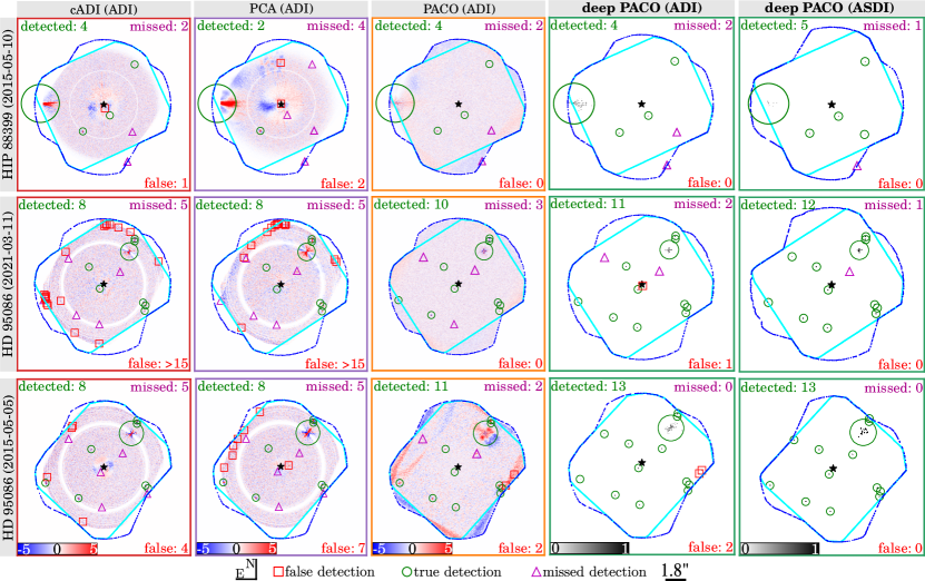
Figure 1: Detection maps obtained with cADI, PCA, PACO, and deep PACO on three datasets (HIP 88399 –2015-05-10–, HD 95086 –2021-03-11–, HD 95086 –2015-05-05–) from the VLT/SPHERE-IRDIS instrument.

For our experiments, we have selected three datasets from the VLT/SPHERE-IRDIS imager [2]. The performance of deep PACO are compared with the cADI, PCA, and PACO algorithms. The details about the observing parameters, the pre-reduction of the recorded datasets, and the setting of the comparative algorithms are discussed in [9, 6].

Figure 1 shows the detection maps obtained with the comparative algorithms. The detected peaks are classified as true, missed, or false detections based on a thresholding of the output map at $\tau=5$ for the algorithms producing a signal-to-noise map (i.e., cADI, PCA, PACO), and at $\tau=0.5$ for deep PACO producing a pseudo-probability map. For the four considered algorithms, the results are obtained by processing the first spectral channel, i.e. exploiting solely ADI. For the proposed approach, we compare ADI and ASDI by also considering a joint processing of the two spectral channels of the dual band observations. These results illustrate the ability of deep PACO to reach, in average, a better detection sensitivity and, at the same time, to avoid some spurious false alarms produced by the comparative algorithms. The joint spectral processing allows to further improve the trade-off between precision and recall.

4 CONCLUSION

As a proof of concept, we applied our method on several datasets from the VLT/SPHERE-IRDIS instrument. We compared the deep PACO method against some state-of-the-art algorithms of the field, including PACO. With ADI, our method reaches in average a better trade-off between precision and recall than the comparative algorithms. A joint processing of spatio-temporo-spectral observations obtained with ASDI allows to further improve the detection performance.

On the methodological side, we are currently investigating ways to improve the deep learning stage of the proposed algorithm by jointly modeling the typical distribution of the nuisance component from multiple datasets. This methodology would strongly differs from reference differential imaging (RDI, [17]) in the sense that a highly non-linear model would be learned from the archived observations and would exploit several prior domain knowledge. On the application side, we will consider to adapt and to apply the deep PACO algorithm on simulated ELT high-contrast data (e.g., from ELT/HARMONI) to ground its benefits in the context of the future giant telescopes.

- [1] Adam Amara and Sascha P Quanz “PYNPOINT: an image processing package for finding exoplanets” In Monthly Notices of the Royal Astronomical Society 427.2 Blackwell Science Ltd Oxford, UK, 2012, pp. 948–955
- [2] J-L Beuzit et al. “SPHERE: the exoplanet imager for the Very Large Telescope” In Astronomy & Astrophysics 631 EDP Sciences, 2019, pp. A155
- [3] Benjamin Charnay et al. “A self-consistent cloud model for brown dwarfs and young giant exoplanets: comparison with photometric and spectroscopic observations” In The Astrophysical Journal 854.2 IOP Publishing, 2018, pp. 172
- [4] Yilun Chen, Ami Wiesel, Yonina C Eldar and Alfred O Hero “Shrinkage algorithms for MMSE covariance estimation” In IEEE Transactions on Signal Processing 58.10 IEEE, 2010, pp. 5016–5029
- [5] Olivier Flasseur, Loic Denis, Éric Thiébaut and Maud Langlois “An unsupervised patch-based approach for exoplanet detection by direct imaging” In IEEE International Conference on Image Processing, 2018, pp. 2735–2739
- [6] Olivier Flasseur et al. “deep PACO: Combining statistical models with deep learning for exoplanet detection and characterization in direct imaging at high contrast” In under minor review in Monthly Notices of the Royal Astronomical Society, 2023
- [7] Olivier Flasseur, Loı̈c Denis, Éric M Thiébaut and Maud Langlois “Exoplanet detection in angular and spectral differential imaging: local learning of background correlations for improved detections” In SPIE Astronomical Telescopes + Instrumentation 10703, 2018, pp. 107032R International Society for OpticsPhotonics
- [8] Olivier Flasseur, Loı̈c Denis, Éric Thiébaut and Maud Langlois “Exoplanet detection in angular differential imaging by statistical learning of the nonstationary patch covariances - The PACO algorithm” In Astronomy & Astrophysics 618 EDP Sciences, 2018, pp. A138
- [9] Olivier Flasseur et al. “Exoplanet detection in angular differential imaging: combining a statistics-based learning with a deep-based learning for improved detections” In Adaptive Optics Systems VIII 12185, 2022, pp. 1154–1167 SPIE
- [10] Olivier Flasseur, Loı̈c Denis, Éric Thiébaut and Maud Langlois “PACO ASDI: an algorithm for exoplanet detection and characterization in direct imaging with integral field spectrographs” In Astronomy & Astrophysics 637 EDP Sciences, 2020, pp. A9
- [11] Olivier Flasseur, Loı̈c Denis, Éric Thiébaut and Maud Langlois “Robustness to bad frames in angular differential imaging: a local weighting approach” In Astronomy & Astrophysics 634 EDP Sciences, 2020, pp. A2
- [12] A-M Lagrange et al. “A probable giant planet imaged in the Pictoris disk: VLT/NaCo deep L’-band imaging” In Astronomy & Astrophysics 493.2 EDP Sciences, 2009, pp. L21–L25
- [13] Olivier Ledoit and Michael Wolf “A well-conditioned estimator for large-dimensional covariance matrices” In Journal of Multivariate Analysis 88.2 Elsevier, 2004, pp. 365–411
- [14] Christian Marois et al. “Angular Differential Imaging: A Powerful High-Contrast Imaging Technique” In The Astrophysical Journal 641.1 IOP Publishing, 2006, pp. 556
- [15] Christian Marois, Carlos Correia, Jean-Pierre Véran and Thayne Currie “TLOCI: A fully loaded speckle killing machine” In Proceedings of the International Astronomical Union 8.S299 Cambridge University Press, 2013, pp. 48–49
- [16] René Racine et al. “Speckle noise and the detection of faint companions” In Publications of the Astronomical Society of the Pacific 111.759 IOP Publishing, 1999, pp. 587
- [17] Garreth Ruane et al. “Reference star differential imaging of close-in companions and circumstellar disks with the, NIRC2 vortex coronagraph at the W.M. Keck observatory” In The Astronomical Journal 157.3 IOP Publishing, 2019, pp. 118
- [18] Rémi Soummer, Laurent Pueyo and James Larkin “Detection and characterization of exoplanets and disks using projections on Karhunen-Loève eigenimages” In The Astrophysical Journal Letters 755.2 IOP Publishing, 2012, pp. L28
- [19] Lu Wang, Chaoli Wang, Zhanquan Sun and Sheng Chen “An improved Dice loss for pneumothorax segmentation by mining the information of negative areas” In IEEE Access 8 IEEE, 2020, pp. 167939–167949