First Resolution of Microlensed Images of a Binary-Lens Event

Abstract

We resolve the multiple images of the binary-lens microlensing event ASASSN-22av using the GRAVITY instrument of the Very Large Telescope Interferometer (VLTI). The light curves show weak binary perturbations, complicating the analysis, but the joint modeling with the VLTI data breaks several degeneracies, arriving at a strongly favored solution. Thanks to precise measurements of angular Einstein radius $\theta_{\rm E}=0.726\pm 0.002$ mas and microlens parallax, we determine that the lens system consists of two M dwarfs with masses of $M_{1}=0.261\pm{0.009}\,M_{\odot}$ and $M_{2}=0.252\pm{0.017}\,M_{\odot}$, a projected separation of $r_{\perp}=7.42\pm 0.33\,{\rm AU}$ and a distance of $D_{\rm L}=2.31\pm 0.09$ kpc. The successful VLTI observations of ASASSN-22av open up a new path for studying intermediate-separation (i.e., a few AUs) stellar-mass binaries, including those containing dark compact objects such as neutron stars and stellar-mass black holes.

1 Introduction

In recent years, the enhanced sensitivity of advanced instrumentation (Eisenhauer et al., 2023) at the Very Large Telescope Interferometer (VLTI) of the European Southern Observatory (ESO) has facilitated interferometric resolution of microlensed images (Delplancke et al., 2001), with the first successful case achieved by Dong et al. (2019) using the GRAVITY instrument (GRAVITY Collaboration et al., 2017). By enabling direct mass determinations, interferometric microlensing opens up a new path into studying Galactic stellar-mass systems, including dark compact objects such as neutron stars and black holes.

The observable effect of microlensing (Einstein, 1936; Paczyński, 1986) is the magnified flux of a background star (i.e., the “source”) due to the gravitational deflection by a foreground object (i.e., the “lens”), and thus microlensing is a sensitive probe to the mass of the lens system, irrespective of its brightness. However, the most easily extracted quantity, the Einstein timescale $t_{\rm E}$ is a degenerate combination of the lens mass $M_{\rm L}$, the lens-source relative parallax $\pi_{\rm rel}$ and the proper motion $\mu_{\rm rel}$,

$$t_{\rm E}=\frac{\theta_{\rm E}}{\mu_{\rm rel}};\quad\theta_{\rm E}\equiv\sqrt{\kappa M_{\rm L}\pi_{\rm rel}};\quad\kappa\equiv\frac{4G}{c^{2}{\rm AU}}\simeq 8.144\frac{{\rm mas}}{M_{\odot}},$$ (1)

where $\theta_{\rm E}$ is the angular Einstein radius, which is on the order of milliarcseconds for stellar-mass microlenses in the Galaxy. To break this degeneracy, a common approach is to measure both $\theta_{\rm E}$ and the so-called “microlens parallax” ${\bm{\pi}}_{\rm E}$ to determine the lens mass (Gould, 2000, 2004),

$$M_{\rm L}=\frac{\theta_{\rm E}}{\kappa\pi_{\rm E}},$$ (2)

where ${\bm{\pi}}_{\rm E}$ is a two-dimensional vector (Gould, 2004) along the same direction as the lens-source relative proper motion vector ${\bm{\mu}}_{\rm rel}$,

$${\bm{\pi}}_{\rm E}\equiv\frac{\pi_{\rm rel}}{\theta_{\rm E}}\frac{{\bm{\mu}}_{\rm rel}}{\mu_{\rm rel}}.$$ (3)

The key advantage of the interferometric microlensing method is that, it yields not only precise $\theta_{\rm E}$ from measuring the angular separation of images, but also constraints on the direction of ${\bm{\pi}}_{\rm E}$.

One often obtains “one-dimensional” microlens parallax from the light curves, that is, the component of ${\bm{\pi}}_{\rm E}$ parallel to the Earth’s acceleration is generally much better constrained than the perpendicular component (Gould et al., 1994; Smith et al., 2003; Gould, 2004). As demonstrated by Dong et al. (2019), Zang et al. (2020), and Cassan et al. (2022), VLTI microlensing can drastically improve the ${\bm{\pi}}_{\rm E}$ measurements from accurate directional constraints via measuring the position angles of images.

A long-adopted method to determine $\theta_{\rm E}$ is via the “finite-source effects” (Gould, 1994a), when the source transits/approaches a caustic (a set of positions that, for a point source, induce infinite magnification). Modeling the finite-source effects in the microlensing light curve measures the ratio between $\theta_{\rm E}$ and the angular radius of the source star $\theta_{*}$, where $\theta_{*}$ can be derived from photometric properties of the source. For a single lens, the caustic is point-like, so finite-source detections in stellar single-lens events are usually restricted to rare cases reaching high peak magnification of $A_{\rm peak}\gtrsim 100$. In contrast, binary lenses have extended caustic structures, and thus, finite-source effects manifest more often in binary-lens events. The first microlens mass measurement by An et al. (2002) is from such a caustic-crossing binary-lens event. However, this method is ineffective for studying events with weak binary perturbations (e.g., non-caustic-crossing). One such weak-binary event was OGLE-2005-SMC-001, for which Dong et al. (2007) detected the space-based microlens parallax (Refsdal, 1966; Gould, 1994b) for the first time, and since no finite-source effects were detected, it was not possible to definitively determine the lens mass due to the absence of a $\theta_{\rm E}$ measurement. While the exact fraction of weak binary events is still an open question, Zhu et al. (2014) predicted and Jung et al. (2022) confirmed that half of planetary events would lack caustic crossings despite their continuous and high-cadence coverages, implying that weak binaries may encompass a significant fraction of binary-lens parameter space.

With milliarcsecond resolution, VLTI can resolve the microlensed images with angular separations around $\gtrsim 2\theta_{\rm E}$ for a stellar-mass-lens microlensing event (Delplancke et al., 2001; Dalal & Lane, 2003; Rattenbury & Mao, 2006; Cassan & Ranc, 2016) and then can determine $\theta_{\rm E}$ at $\sim\%$ precision. Dong et al. (2019) measured $\theta_{\rm E}=1.87\pm 0.03\,{\rm mas}$ for TCP J05074264+2447555 (a.k.a., Kojima-1) with VLTI GRAVITY, leading to a mass measurement of $M_{\rm L}=0.495\pm 0.063\,M_{\sun}$ when combined with microlens parallax (Zang et al., 2020). Cassan et al. (2022) obtained $\theta_{\rm E}=0.7650\pm 0.0038\,{\rm mas}$ for Gaia19bld (Rybicki et al., 2022) with VLTI-PIONIER (Le Bouquin et al., 2011) and then determined that $M_{\rm L}=1.147\pm 0.029\,M_{\sun}$. Both events were exceptionally bright since VLTI microlensing observations were limited by the instrument’s sensitivity, with $K\lesssim 10.5$ for the on-axis mode of GRAVITY and $H\lesssim 7.5$ for PIONIER. GRAVITY has been recently upgraded to enable dual-beam capability (known as “GRAVITY Wide”, GRAVITY+ Collaboration et al. 2022a) with a boosted sensitivity, and using GRAVITY wide, Mróz et al. (2024) measured that OGLE-2023-BLG-0061/KMT-2023-BLG-0496 has $\theta_{\rm E}=1.280\pm 0.009$ mas and inferred its lens mass $M_{\rm L}=0.472\pm 0.012\,{\rm M_{\odot}}$. Future upgrades to GRAVITY+ are expected to significantly improve the sensitivity (GRAVITY+ Collaboration et al., 2022b) and consequently the number of accessible microlensing events.

The VLTI-microlensing observations published so far have been exclusively on single-lens events (or hosts of extremely low-mass companions). Here, we analyze ASASSN-22av, the first binary-lens microlensing event with multiple images resolved by VLTI.

2 Observations and Data Reduction

ASASSN-22av was discovered as a microlensing event candidate on UT 2022-01-19.10 by the All-Sky Automatic Survey for Supernovae (ASAS-SN; Shappee et al., 2014). Its Gaia DR3 (Gaia Collaboration et al., 2023) source_id is 5887701839850363776 and coordinates are $(\alpha,\delta)_{\rm J2000}=(15^{\rm h}01^{\rm m}00.66^{\rm s},-54\arcdeg 23\arcmin 59.96\arcsec)$, corresponding to Galactic coordinates $(l,b)_{\rm J2000}=(321.14522^{\circ},3.82467^{\circ})$. Following its discovery, we modeled the real-time ASAS-SN light curve (Kochanek et al., 2017) and found that it was consistent with a point-source point-lens (PSPL; Paczyński 1986) model reaching a peak magnification of $A_{\rm peak}\sim 20$–$30$ around UT 2022-01-20. Its baseline is at $K_{s}=9.27\pm 0.02$ (2MASS ID: J15010066$-$5423599) and $G=13.82$, and the magnified brightness was well above the limit for conducting on-axis GRAVITY observations with Multi-Application Curvature Adaptive Optics (MACAO).

We began to conduct VLTI GRAVITY observations in the night of UT 2022-01-21, and subsequently made ongoing observations until 2022-01-25. We discuss the VLTI observations and data reduction in § 2.1. We also started photometric follow-up observations on UT 2022-01-20 (see § 2.2 for detailed descriptions of photometric data). On UT 2022-01-21, our light-curve modeling suggested significant deviations from the best-fit PSPL model, and we found that a finite-source point-lens (FSPL) model was now preferred. Aiming at performing “stellar atmosphere tomography” (see, e.g., Albrow et al., 2001; Afonso et al., 2001, and references therein) near the caustic exit, we initiated a campaign of time-series high-resolution spectroscopy. On UT 2022-01-24, we noticed that the light curve declined faster than expected from the best-fit FSPL model and considered the possibility of a binary-lens perturbation, which was confirmed by our later analysis (see § 3 for detailed discussions on light-curve modeling). We obtained high-resolution spectra from the High Resolution Spectrograph (HRS) on the Southern African Large Telescope (SALT; Buckley et al. 2006), the MIKE spectrograph (Bernstein et al., 2003) on the Magellan Clay 6.5 m telescope, the High Efficiency and Resolution Multi Element Spectrograph (HERMES; Sheinis et al. 2015) on the Anglo-Australian Telescope (AAT), and the HARPS spectrograph (Mayor et al., 2003) on the ESO’s 3.6 m telescope from UT 2022-01-25 to UT 2022-01-30. The full description of the spectroscopic data and the stellar atmosphere tomography analysis will be presented in a future paper. In this work, we utilize the stellar parameters of the source extracted from the HERMES data presented in § 2.3.

2.1 Interferometric Data

We observed ASASSN-22av with the VLTI GRAVITY instrument (GRAVITY Collaboration et al., 2017) on the four nights of 21, 22, 24, and 25 January 2022. The observations were executed with the single-field on-axis mode at medium-resolution ($R=\lambda/\Delta\lambda\simeq 500)$. We use all data except those on 2022/01/21 when there was significant flux loss in UT2 and poor fringe-tracking performance. The remaining three nights of data are reduced with the standard GRAVITY pipeline (version 1.6.6), and there are 2, 4, and 2 exposures in the nights of 22, 24 and 25, respectively. Throughout this paper, we refer to these three nights as Nights 1, 2, and 3, respectively. We first use the Python script run_gravi_reduced.py to reduce the raw data up to the application of the pixel-to-visibility matrix (P2VM). The default options are used except for adopting --gravity_vis.output-phase-sc=SELF_VISPHI to calculate the internal differential phase between each spectral channel. The pipeline performed the bias and sky subtraction, flat fielding, wavelength calibration, and spectral extraction. Application of the P2VM converts the pixel detector counts into complex visibilities, taking into account all instrumental effects, including relative throughput, coherence, phase shift, and cross-talk. The dark, bad pixel, flat field, wavelength calibration, and P2VM matrix data are reduced from the daily calibration data obtained close in time to our observations. We then use run_gravi_trend.py to calibrate the closure phase with the calibrator observation of HD134122 next to the science target observations.

The observations employed 4 UTs and thus there are four closure phases for every spectral channel. In principle, the four closure phases are not independent and should sum up to zero. We examine the calibrator data and find that the standard deviation of the sum of the closure phases is $\sim 0.15^{\circ}$, comparable to the pipeline-reported closure phase uncertainties in the science data. Thus, we take the simplified approach and treat the four closure phases as uncorrelated observables rather than the more sophisticated approach of treating the correlated noise employed by Kammerer et al. (2020). On each night, we have two exposures for the calibrator star, and we find the closure phase differences of the two exposures have scatters of $0.21^{\circ},0.25^{\circ},0.35^{\circ}$ on Night 1, 2 and 3, respectively. We adopt these values as the uncertainties introduced in the calibration process and add them quadratically to the closure-phase errors.

The medium-resolution spectrograph samples 233 wavelengths spanning $2.0-2.4\,\rm um$. To speed up computation, the 233 closure phases are binned into 10 phases in our modeling process. The first and last phases are discarded due to the low signal-to-noise ratio and significant deviation from the model. See Appendix A for the description of the binning process.

2.2 Photometric Data

We obtained follow-up imaging data taken with 1-m telescopes of Las Cumbres Observatory Global Telescope Network (LCOGT; Brown et al., 2013) in the Sloan $g^{\prime}r^{\prime}i^{\prime}$ filters, the 0.4-m telescope of Auckland Observatory (AO) at Auckland (New Zealand) in the $g^{\prime}r^{\prime}i^{\prime}$ filters, and the 30-cm Perth Exoplanet Survey Telescope (PEST) in the $g^{\prime}r^{\prime}i^{\prime}$ filters.

We use the PmPyeasy pipeline (Chen et al., 2022) to do the photometry on these follow-up images. For LCOGT and PEST data, we conduct image subtractions with the hotpants code (Becker, 2015), and then we employ aperture photometry on the subtracted images. For the AO data, we performed point-spread-function (PSF) photometry using DoPHOT (Schechter et al., 1993).

We co-added and analyzed the $g^{\prime}$-band ASAS-SN images using the standard ASAS-SN photometric pipeline based on the ISIS image-subtraction code (Alard & Lupton, 1998; Alard, 2000). The baseline ($g^{\prime}\sim 15.5$) is too faint to obtain precise photometry for ASAS-SN, and we analyze the magnified ASAS-SN epochs with ${\rm HJD^{\prime}=HJD}-2450000\in(9577.857,9677.608)$. There are data from three ASAS-SN cameras (be, bi and bm), and they are analyzed independently in the modeling.

This event was announced as Gaia22ahy by Gaia Science Alerts (GSA; Hodgkin et al., 2021) on UT 2022-01-25.4. The Gaia $G$-band light curve available on GSA website does not have uncertainties, and we adopt the same error bar ($\sigma_{G}=0.02$) for all data points. We noticed that the data in 2015 exhibit systematically larger scatter than the rest of the Gaia baseline. By inspecting a few other GSA microlensing light curves (Wyrzykowski et al., 2023), we found similar patterns at the beginning of the Gaia mission, possibly due to the continued contamination by water ice (Gaia Collaboration et al., 2016). We conservatively remove all Gaia data before the last decontamination run on 2016/08/22 (Riello et al., 2021) from our analysis.

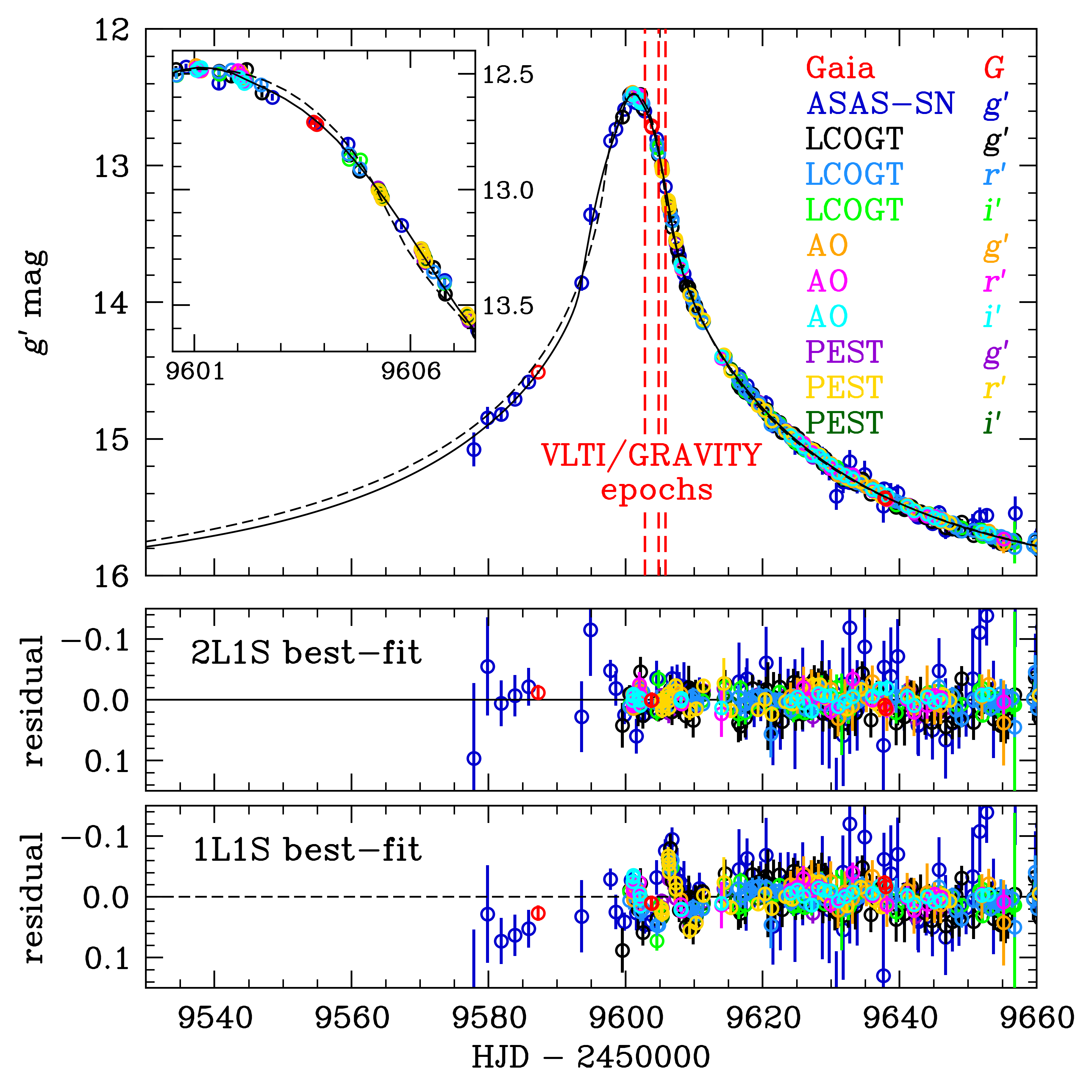
Figure 1: Top: The multi-band light curves of the microlensing event ASASSN-22av, which are well described by the best-fit 2L1S model (black solid line) from the joint VLTI and light-curve analysis. The light curves deviate from the best-fit 1L1S model with finite-source effects (black dashed line) near the peak, as shown with the enlarged view in the inset. We analyze three nights of VLTI GRAVITY observations taken after the peak, and their epochs are marked with the red dashed lines. Middle: The residuals of the best-fit 2L1S model. Bottom: The best-fit 1L1S model shows significant residuals for the $\sim 10$ days around the peak.

We follow the standard procedure (Yee et al., 2012) of re-normalizing the error bars such that $\chi^{2}/{\rm d.o.f}$ is unity for each data set for the best-fit model. We reject the 3 $\sigma$ outliers and thereby exclude 4 out of 983 photometric data points from the analysis (the rejected data consist of one data point each from LCOGT $r^{\prime}$ and $i^{\prime}$, and one epoch each from the ASAS-SN bi and bm cameras). Figure 1 shows the multi-band light curves of ASASSN-22av.

2.3 HERMES Spectroscopic Data & Stellar Parameters

We obtained a high-resolution optical spectrum (sobject_id 220125001601051) on UT 2022-01-25.75 as part of ongoing observations of the Galactic Archaeology with HERMES survey (De Silva et al., 2015, hereafter GALAH). The total exposure time is 3600 s. The HERMES spectrograph on the 3.9-m Anglo-Australian Telescope at Siding Spring Observatory covers four wavelength regions (4713–4903, 5648–5873, 6478–6737, and 7585–7887 Å) that can show absorption features from up to 31 elements, including the two strong Balmer lines $\mathrm{H\alpha}$ and $\mathrm{H\beta}$.

We use the observations and analysis of the most recent analysis cycle, which will be published as the fourth GALAH data release (DR4; Buder et al., in preparation). The spectra are reduced using a similar analysis to the third data release (Buder et al., 2021) with a custom-built reduction pipeline (Kos et al., 2017). Stellar parameters, that is, effective temperature ($T_{\mathrm{eff}}$), surface gravity ($\log g$), radial, microturbulence and rotational velocities ($v_{\mathrm{rad}}$, $v_{\mathrm{mic}}$ and $v\sin i$), as well as up to 31 elemental abundances, are then simultaneously estimated by minimizing the weighted residuals between the observed and synthetic stellar spectra. The latter are interpolated with a high-dimensional neural network (compare to Ting et al., 2019) trained on synthetic stellar spectra generated with the spectrum synthesis code Spectroscopy Made Easy (Piskunov & Valenti, 2017), and degraded to the measured instrumental resolution of the spectrum. This change with respect to the third data release, which used wavelength regions of carefully selected unblended lines, allows 94% of the observed wavelength range to be used and thus considerably increases the measurement precision.

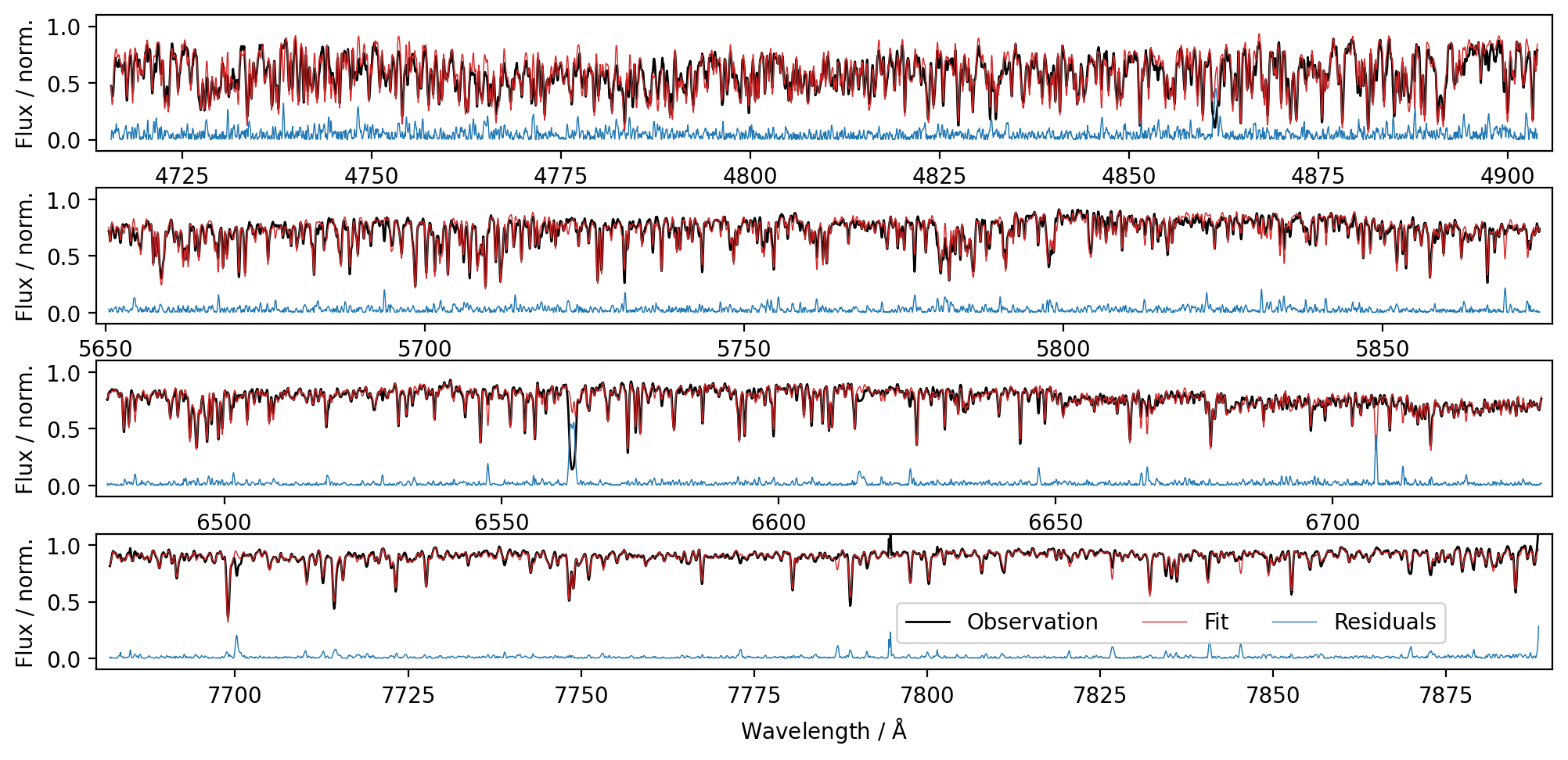
Figure 2: The observed (black) and fitted (red) synthetic HERMES spectrum from GALAH Data Release 4, showing generally good agreements and small residuals (blue) across the entire spectrum. While some individual lines are deviating, the overall fit is well aligned with the observations whose continuum is suppressed by molecular absorption features across the entire wavelength region of this luminous cool giant star.

The spectroscopic fit also includes photometric and astrometric information from the 2MASS (Skrutskie et al., 2006) and Gaia surveys (Lindegren et al., 2021) to constrain the surface gravity. This leads to more accurate stellar parameters, as shown in the previous HERMES analyses (Buder et al., 2018, 2019, 2021), particularly for cool giant stars such as the target of this study, where molecular features complicate the spectroscopic analysis. The fit is very good with the signal-to-noise ratio increasing across the four wavelength regions (16, 107, 194, and 254), as can be seen from Figure 2. We do not expect a good fit to the Balmer line cores or the lithium lines at $4861$, $6563$, and $6708\,\text{\AA}$, respectively. No quality concerns are raised by the automatic pipeline (flag_sp = 0).

The final radial velocity of $v_{\mathrm{rad}}=-72.44\pm 0.18\,\mathrm{km\,s^{-1}}$ is in very good agreement with the value from the Gaia DR3 spectrum, that is, $v_{\mathrm{rad},Gaia}=-71.8\pm 1.0\,\mathrm{km\,s^{-1}}$ (Recio-Blanco et al., 2023). The final stellar parameters are $T_{\mathrm{eff}}=3776\pm 67\,\mathrm{K}$, $\log g=1.05\pm 0.12$, $\mathrm{[Fe/H]}=-0.148\pm 0.053$, $v_{\mathrm{mic}}=1.82\pm 0.28\,\mathrm{km\,s^{-1}}$, and $v\sin i=5.5\pm 1.4\,\mathrm{km\,s^{-1}}$. The stellar abundances are close to the Solar values, for example, $\mathrm{[Mg/Fe]}=0.007\pm 0.011$.

3 Light-Curve Analysis

3.1 Single-lens Model

In a microlensing event, the flux is modeled as

$$f(t)=f_{\rm S}\cdot A(t)+f_{\rm B},$$ (4)

where $A(t)$ is the magnification as a function of time, and $f_{\rm S}$ and and $f_{\rm B}$ are the source flux and the blended flux within the PSF, respectively. In the simplest single-lens single-source (1L1S) model, i.e., the PSPL model (Paczyński, 1986), the magnification is given by,

$$A_{\rm PSPL}=\frac{u^{2}+2}{u\sqrt{u^{2}+4}};\qquad u(t)=\sqrt{u_{0}^{2}+\frac{(t-t_{0})^{2}}{t_{\rm E}^{2}}},$$ (5)

where $u$ is the angular lens-source separation normalized by $\theta_{\rm E}$, and ($t_{0}$, $u_{0}$) are the time of the closest source-lens approach and the impact parameter normalized by $\theta_{\rm E}$, respectively.

The peak of the light curve (Figure 1) is flattened compared to the PSPL model, suggesting possible finite-source effects (Gould, 1994a). We fit the finite-source point-lens (FSPL) model to the light curve by introducing an additional parameter $\rho={\theta_{*}}/{\theta_{\rm E}}$. In the FSPL model, $A_{\rm FSPL}$ is calculated by integrating the $A_{\rm PSPL}$ over a limb-darkened source disk. Using the best-fit spectroscopic parameters (see § 2.3), we estimate the limb-darkening coefficients $(\Gamma_{g^{\prime}},\Gamma_{r^{\prime}},\Gamma_{i^{\prime}},\Gamma_{G})=(0.91,0.77,0.63,0.74)$ based on Claret & Bloemen (2011) and Claret (2019).

The best-fit FSPL model is shown as a dashed black line in the top panel of Figure 1, and the residuals are shown in the bottom panel. The residuals exhibit significant trends deviating from the FSPL model, spanning $\sim 10$ days around the peak. These systematic deviations cannot be absorbed by adjusting either the limb-darkening coefficients or the free parameters in the FSPL models.

3.2 Binary-lens Model

The light curve can be well described by the binary-lens single-source (2L1S) model. We start the analysis with the static binary-lens model, which includes three additional parameters $(s,q,\alpha)$ to describe a non-rotating binary-lens systems: $s$ is the projected angular separation of the binary components normalized by $\theta_{\rm E}$, $q$ is the binary mass ratio, and $\alpha$ is the angle between the source-lens trajectory and the binary-lens axis. We use the advanced contour integration package VBBinaryLensing (Bozza, 2010; Bozza et al., 2018) to calculate the binary-lens magnification $A(t,\Theta_{\rm 2L1S})$ given the parameters $\Theta_{\rm 2L1S}=\{s,q,\alpha,\rho,t_{0},u_{0},t_{\rm E}\}$.

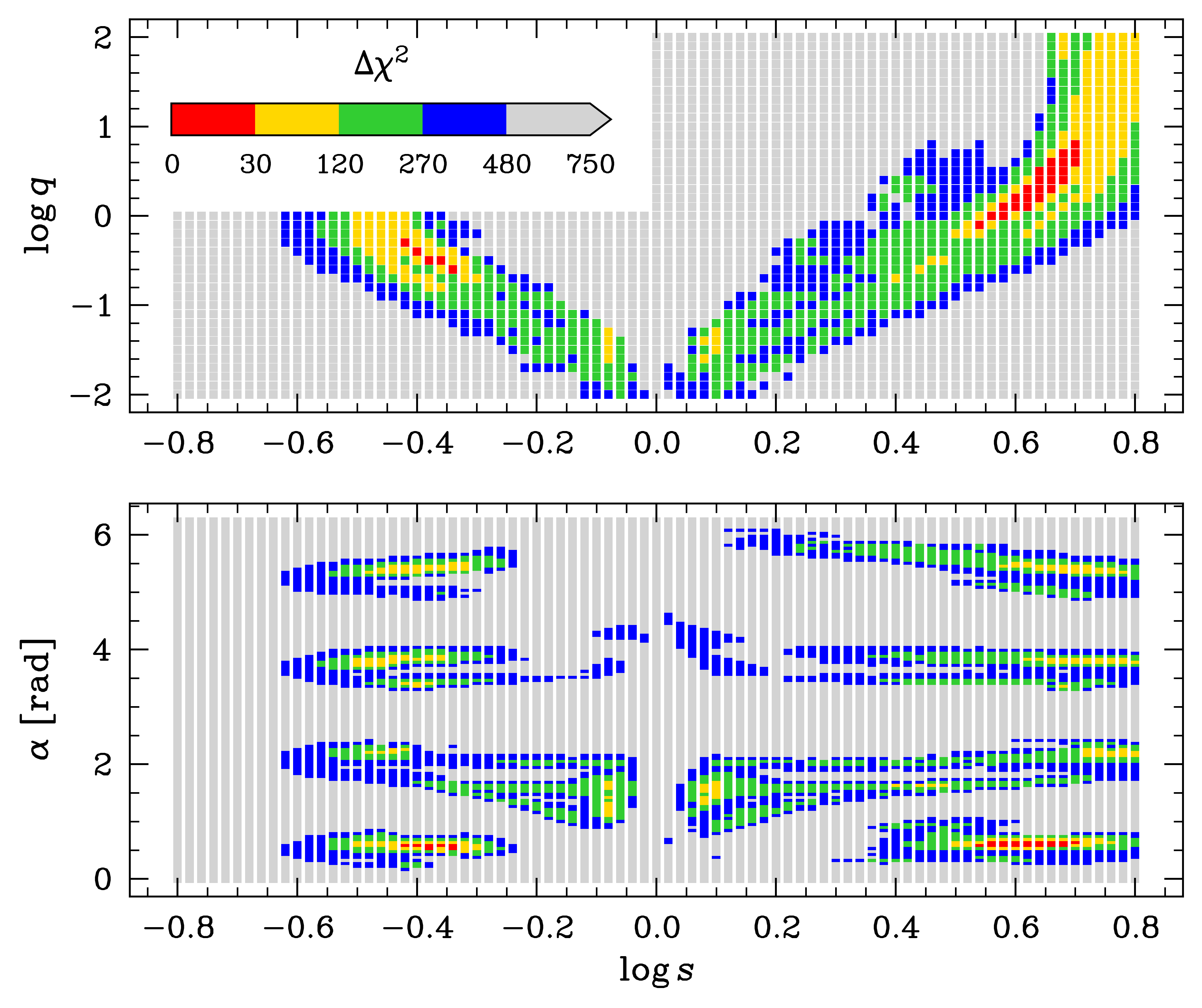
Figure 3: $\Delta\chi^{2}$ map for the grid search of 2L1S light-curve models, in the $\log s-\log q$ (upper panel) and $\log s-\alpha$ planes (lower panel). For $\log s<0$, there is a perfect degeneracy $(\log q,\alpha)\to(-\log q,\alpha+\pi)$, and thus the search is only conducted with $\log q\leq 0$. The regions with $\Delta\chi^{2}<30,120,270,480$ and $>480$ with respect to the best fit are color-coded with red, yellow, green, blue and light gray, respectively.

We start by scanning the 7-d parameter space on a fixed $(\log s,\log q,\alpha)$ grid with $-1\leq\log s\leq 1$, $-2\leq\log q\leq 1$ and $0\leq\alpha<2\pi$. At each grid point, we minimize the $\chi^{2}$ by setting the 4 remaining parameters $(t_{0},u_{0},t_{\rm eff}\equiv u_{0}t_{\rm E},t_{*}\equiv\rho t_{\rm E})$ free in MCMC using the EMCEE package (Foreman-Mackey et al., 2013). The resulting $\chi^{2}$ map is shown in Figure 3, from which we identify 5 local minima in the close-binary $(s<1)$ regime and 9 local minima in the wide-binary $(s>1)$ regime. The severe finite-source effects smear out the sharp magnification structure of caustics, leading to a plethora of local minima over a broad range of $\log q$. For close solutions, there is a perfect degeneracy of $(\log q,\alpha)\to(-\log q,\alpha+\pi)$, and therefore we only conduct the grid search with $\log q\leq 0$. For wide solutions, we have a 4-fold degeneracy in $\alpha$. When $q\gg 1$, the “planetary” caustic associated with secondary mass is reduced to a Chang-Refsdal (Chang & Refsdal, 1979) caustic with shear $s^{-2}/q\ll 1$. The four identical cusps of a Chang-Refsdal lead to a degeneracy of $\alpha\to\alpha+\pi/2$, as shown in Figure 3. The solutions with $q\gg 1$ can correspond to unrealistic value of $t_{\rm E}$. We limited our analysis to $\log q<3$, which corresponds to an upper limit of $t_{\rm E}\sim 2000\,\rm d$.

Then we probe all local minima by setting all the parameters free in MCMC. We also introduce the higher-order effects into the modeling. We include the annual microlens parallax effects (Gould, 1992), which are the light-curve distortions due to the Earth’s orbital acceleration toward the Sun. The static binary-lens model has a perfect geometric degeneracy $(u_{0},\alpha)\to-(u_{0},\alpha)$, which is broken when taking the microlens parallax into account. For the $u_{0}>0$ and $u_{0}<0$ geometry, the lens takes different sides of the source trajectory, leading to different magnifications. The microlens parallax effects are described by ${\bm{\pi}}_{\rm E}$ vector with the East and North components ${\bm{\pi}}_{\rm E}=(\pi_{\rm E,E},\pi_{\rm E,N})$, as defined in Gould (2004). We also consider the orbital motion of the binary lens, which can have degeneracies with microlens parallax (Batista et al., 2011; Skowron et al., 2011). We apply the linearized orbital motion

$$s(t)=s_{0}+\frac{ds}{dt}(t-t_{0});\;\;\;\alpha(t)=\alpha_{0}+\frac{d\alpha}{dt}(t-t_{0}).$$ (6)

with two parameters $ds/dt$ and $d\alpha/dt$. This approximation is subject to physical constraints as discussed in Dong et al. (2009). For a bound system, the ratio of the projected kinetic to the potential energy $\beta$ should be less than unity:

$$\beta=\left|\frac{\rm KE_{\perp}}{\rm PE_{\perp}}\right|=\frac{(\gamma\cdot{\rm yr})^{2}}{8\pi^{2}}\frac{M_{\sun}\kappa\pi_{\rm E}}{\theta_{\rm E}}\left(\frac{s}{\pi_{\rm E}+\pi_{\rm S}/\theta_{\rm E}}\right)^{3}<1,$$ (7)

where $\gamma=(ds/s\,dt,d\alpha/dt)$ and $\pi_{\rm S}$ is the trigonometric parallax of the source star. We adopt $\theta_{\rm E}=0.73\,{\rm mas}$ and $\pi_{\rm S}=0.185\,{\rm mas}$ (see § 5.1) and restrict the MCMC exploration to $\beta<1$.

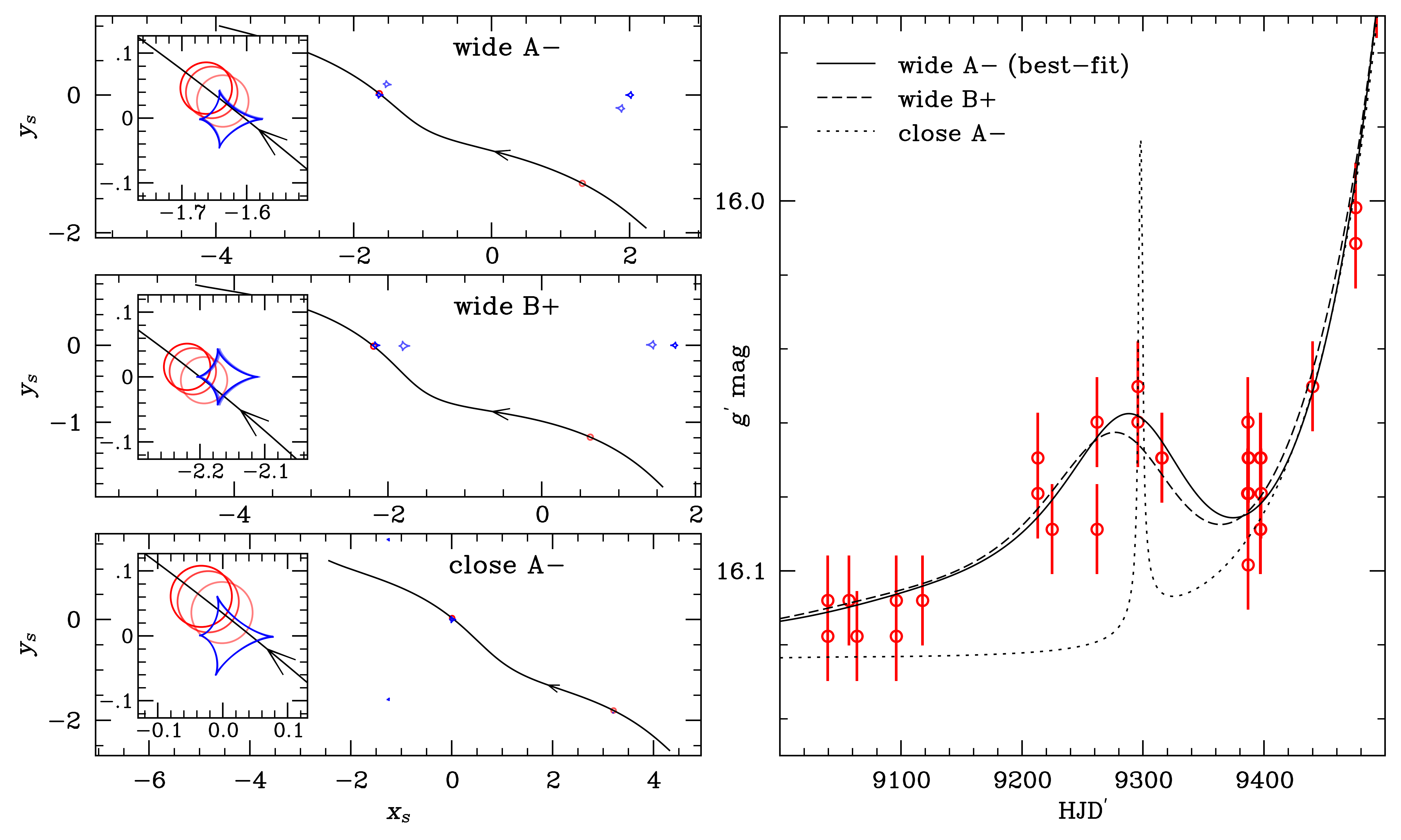
Figure 4: The source trajectories and light curves of three 2L1S models (“wide A$-$”, “wide $B+$” and “close A$-$”) taking the microlens parallax and binary orbital motion into account. Left: The upper, middle, and lower sub-panels show the caustics (blue) and source trajectories (black curves with arrows) for the “wide A$-$” (best-fit), “wide B$+$”, and “close A$-$” solutions, respectively. In each sub-panel, we show the source positions (red circles) and caustics at $\rm HJD^{\prime}=9300$ and $9601$, with increased opacity for the latter. The inset of each subpanel displays the source positions and caustics at the three nights of VLTI GRAVITY observations. Right: The Gaia $G$ light curve shows a broad feature at $\rm HJD^{\prime}\sim 9300$, and the three best-fit 2L1S models are shown with solid (wide A$-$), dashed (wide B$+$), and dash-dot (close A$-$) lines, respectively. The wide solutions can match this feature well while the “close A$-$” solution cannot.

We find that the best-fit solution is a wide-binary with $u_{0}<0$ and label it as “wide A$-$”. The source trajectory and caustics are shown in the upper left sub-panel of Figure 4. The “wide A$-$” solution has $\chi^{2}=948.9$, and all other solutions are worse by $\Delta\chi^{2}>50$. Nevertheless, we keep all solutions with $\Delta\chi^{2}<81$ (listed in Table 1) for further analysis incorporating the VLTI GRAVITY data.

4 Interferometric Data Analysis

4.1 Parameterization

The images generated from the binary-lens equation are oriented with respect to the binary-lens axis and in the units of the Einstein radius, so they need to be rotated to the sky plane and scaled by $\theta_{\rm E}$ to compute the closure phases. We define $\Psi$ as the position angle of the binary-lens axis. The direction of lens-source relative motion ${\bm{\mu}}_{\rm rel}$ , which is the same as that of the microlens parallax ${\bm{\pi}}_{\rm E}$, can be expressed as:

$$\Phi_{{\bm{\pi}}}=\alpha+\Psi$$ (8)

We incorporate the 2 parameters $\{\theta_{\rm E},\Psi\}$ in addition to the 2L1S parameters $\{s,q,\alpha,\rho,t_{0},u_{0},t_{\rm E}\}$ for modeling the interferometric data. The microlens parallax is re-parameterized by $(\pi_{\rm E,N},\pi_{\rm E,E})=\pi_{\rm E}\cdot(\cos\Phi_{{\bm{\pi}}},\sin\Phi_{{\bm{\pi}}})$ with $\Phi_{{\bm{\pi}}}=\alpha+\Psi$.

4.2 Probing Interferometric Observables

Prior to carrying out the full joint analysis of VLTI and light curve, we first investigate the VLTI observables with limited input from the light-curve models. We start the investigation using only $(s,q,\rho)$ from the best-fit light-curve model “wide A$-$”. We perform 4-dimensional grid search on $(\theta_{\rm E},\Psi,u_{x},u_{y})$ to fit the closure-phase data from each of the eight VLTI exposures, where $(u_{x},u_{y})$ are the source’s coordinates on the binary-lens plane. At each grid point, we generate the images scaled and rotated to the sky plane based on $(\theta_{\rm E},\Psi)$ and then calculate the closure phases and corresponding $\chi_{{\rm VLTI},i}^{2}(\theta_{\rm E},\Psi,u_{x},u_{y})$ for every VLTI exposure $i$. We describe our method of calculating the closure phase from the binary-lens images in Appendix B. Our closure-phase calculations from the images are validated with the PMOIRED software (Mérand, 2022).

To exclude unreasonable source positions, we add a penalty term

$$\chi^{2}_{i}=\chi_{{\rm VLTI},i}^{2}+\left(\frac{A(u_{x,i},u_{y,i})-A_{{\rm LC},i}}{0.1A_{{\rm LC},i}}\right)^{2},$$ (9)

for the deviation from light-curve magnification for each VLTI exposure $i$, where $A_{{\rm LC},i}$ is the magnification from the “wide A$-$” model at the $i$-th VLTI exposure, and we adopt a fractional error of $10\%$ so that $(u_{x,i},u_{y,i})$ are only subject to loose light-curve magnification constraints.

A self-consistent VLTI model should have the same values of $(\theta_{\rm E},\Psi)$ on all the exposures. Therefore, for each set of $(\theta_{\rm E},\Psi)$, we calculate

$$\chi_{\rm tot}^{2}(\theta_{\rm E},\Psi)=\sum_{i}{\rm min}\left[\chi_{i}^{2}(\theta_{\rm E},\Psi,u_{x,i},u_{y,i})\right],$$ (10)

where ${\rm min}\left[\chi_{i}^{2}(\theta_{\rm E},\Psi,u_{x,i},u_{y,i})\right]$ is the minimum $\chi^{2}$ for a given $(\theta_{\rm E},\Psi)$ in the $i$-th VLTI exposure.

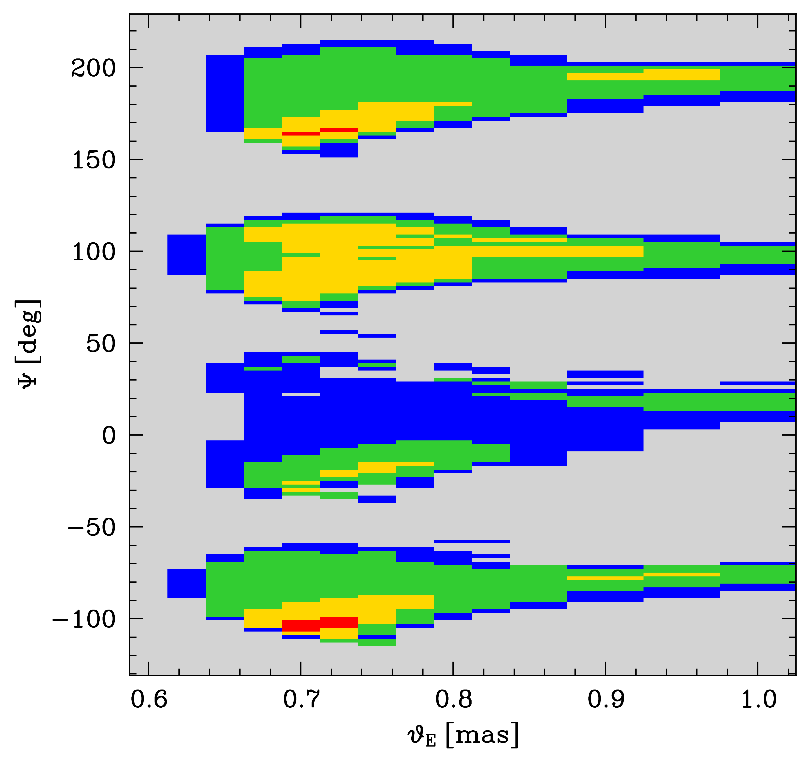
(a)

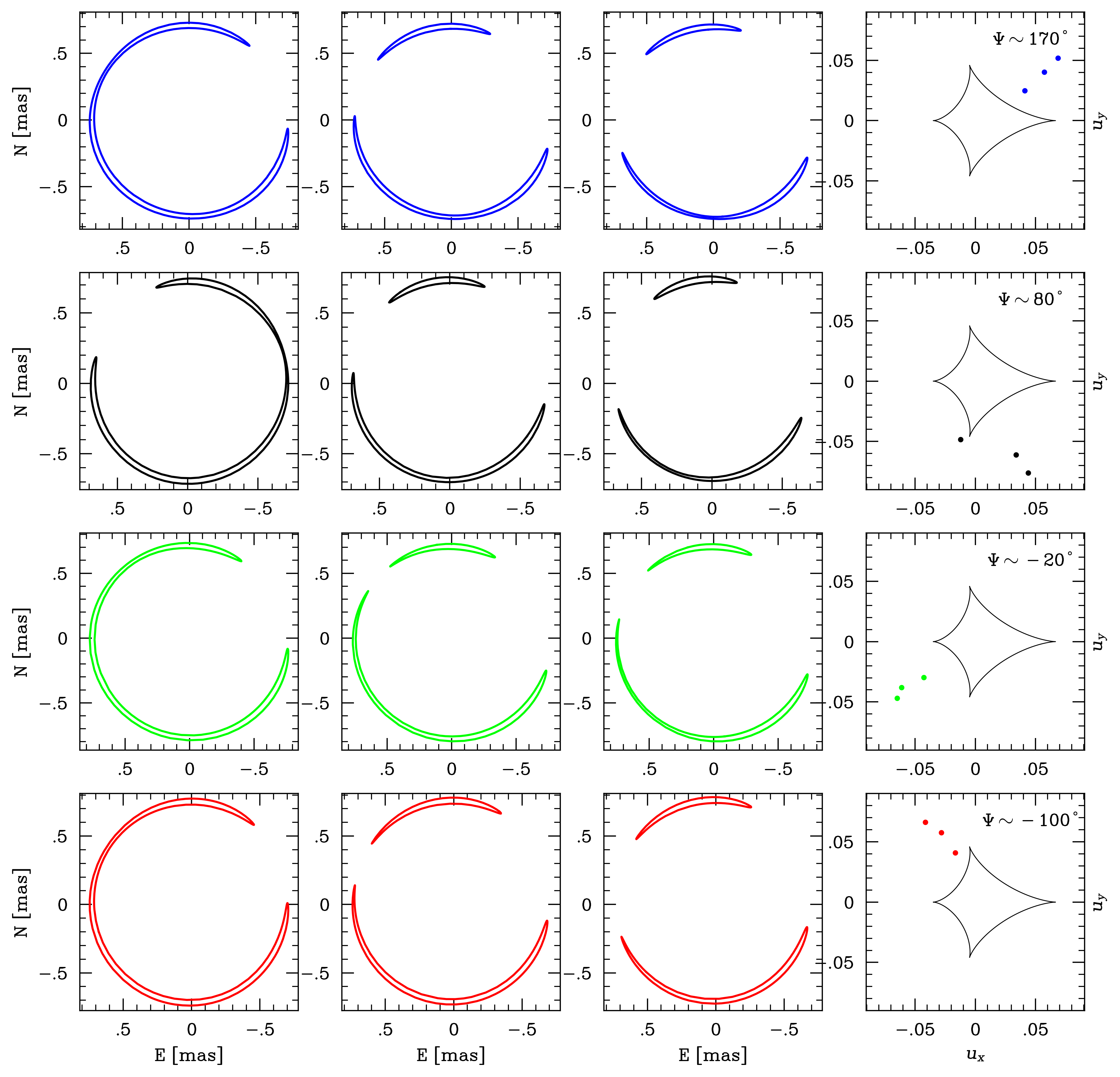
(b)

Figure 5: Left: The $\Delta\chi_{\rm tot}^{2}(\theta_{\rm E},\Psi)$ map from fitting the VLTI data evaluated at $(s,q,\rho)=(3.8,0.84,0.044)$. Areas with $\Delta\chi^{2}<30,120,270,480$ and $\Delta\chi^{2}>480$ are color-coded in red, yellow, green, blue, and gray, respectively. There are four local minima around $\Psi=(170^{\circ},80^{\circ},-10^{\circ},-100^{\circ})$ Right: Images and geometry of the four local minima. The four rows from top to bottom correspond to local minima at $\Psi=170^{\circ}(\rm blue),80^{\circ}(\rm black),-10^{\circ}(\rm green),-100^{\circ}(\rm red)$, respectively. The first three columns show the model images oriented in the East and North directions on the three VLTI nights. The last column shows the source positions (solid dots) on the three VLTI nights and the caustics (black closed curve).

The left panel of Figure 5 shows the $\Delta\chi^{2}_{\rm tot}(\theta_{\rm E},\Psi)$ map, from which we identify four local minima. The $\theta_{\rm E}$ is within a broad range of $0.6-1.0\,{\rm mas}$, and $\Psi$ is subject to a 4-fold degeneracy around $(-100^{\circ},-10^{\circ},80^{\circ},170^{\circ})$, each with an uncertainty of $\sim 10^{\circ}$. The 4-fold degeneracy corresponds to having the source positions near the four cusps of the “central” caustic associated with the primary mass, resulting in similar image morphologies that are compatible with the VLTI data (see the sub-panels on the right of Figure 5).

Next, we further probe the four local minima by jointly fitting all epochs of VLTI data. In a satisfactory VLTI microlensing model, the source positions should lie approximately on a straight line following the source-lens relative motion, so we parameterize the source positions $(u_{x},u_{y})$ with $(u_{0},t_{0},t_{\rm E},\alpha)$ as,

$$u_{x} =u_{0}\sin\alpha-\tau\cos\alpha,$$

$$u_{y} =-u_{0}\cos\alpha-\tau\sin\alpha,$$

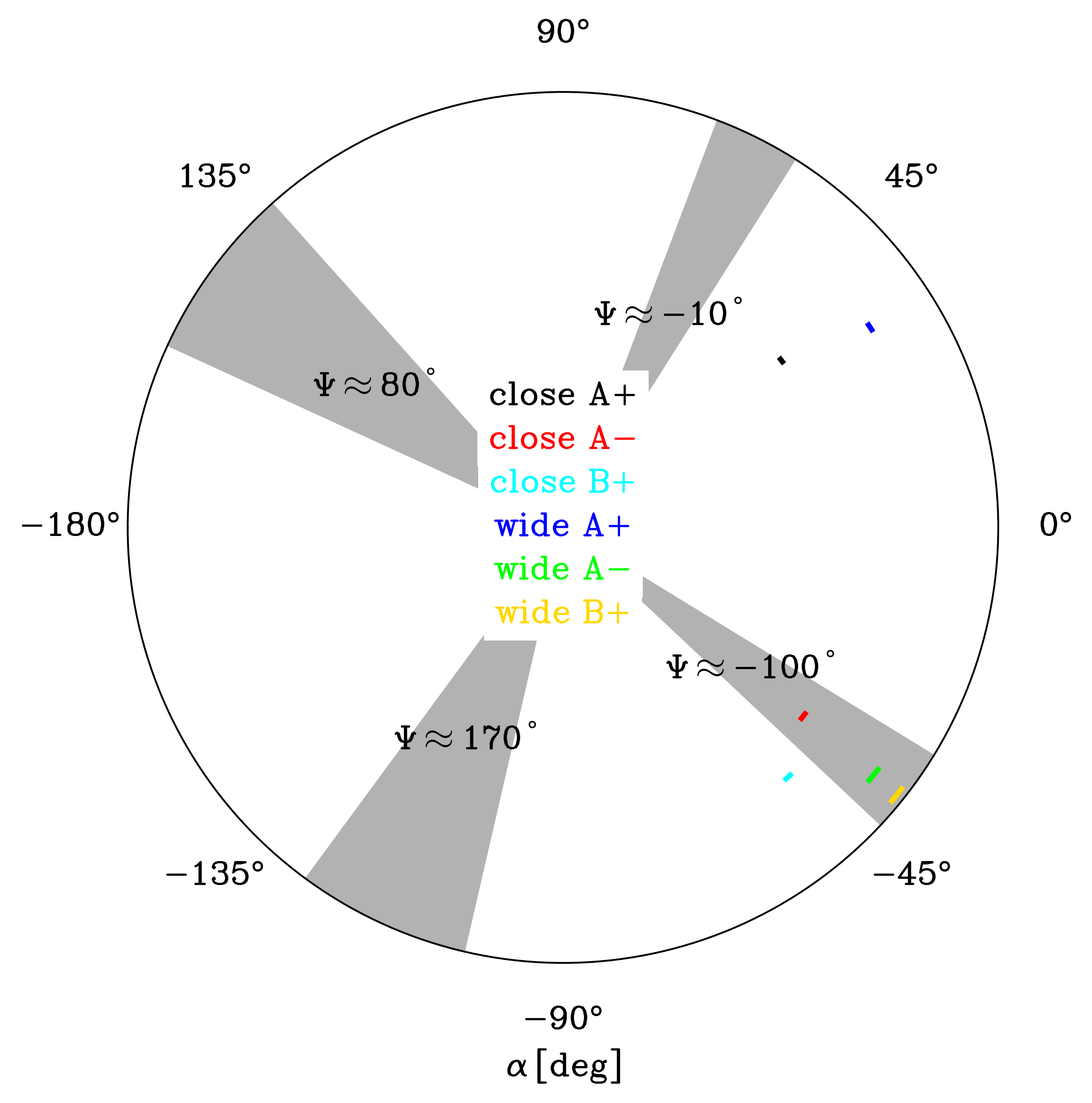
Figure 6: The comparisons of $\alpha_{\rm LC}$ derived from light-curve fitting with $\alpha_{\rm VLTI}$ inferred from VLTI data. The colored arcs denote the 1$\sigma$ range of $\alpha_{\rm LC}$ for solutions “close A$+$” (black), “close A$-$” (red), “close B$+$” (cyan), “wide A$+$” (blue), “wide A$-$” (green) and “wide B$+$” (yellow), respectively. The shaded regions indicate the 3$\sigma$ range of $\alpha_{\rm VLTI}$ at $\Psi\sim-100^{\circ},-10^{\circ},80^{\circ}$ and $170^{\circ}$. Three solutions (wide A$-$, wide B$+$ and close A$-$) have consistent $\alpha_{\rm LC}$ with $\alpha_{\rm VLTI}$.

where $\tau=(t-t_{0})/{t_{\rm E}}$. The interferometric parameters $(\theta_{\rm E},\Psi)$ are seeded from the above-mentioned four local minima. We allow $(\log s,\log q,\log\rho)$ to freely vary, and no longer add the $\chi^{2}$ penalty term as in Eq. 9. The four best-fit solutions have similar $\chi^{2}$ ($\Delta\chi^{2}<10$), so the VLTI data alone cannot distinguish between them. All the solutions strongly prefer $u_{0}<0$. As in the previous single-lens events, $u_{0}>0$ and $u_{0}<0$ solutions can distinguished with two or more epochs of VLTI data (Dong et al., 2019; Zang et al., 2020; Cassan et al., 2022). The four degenerate solutions correspond to 4 distinct $\alpha$ values, denoted as $\alpha_{\rm VLTI}$, which are displayed as shaded regions in Figure 6. The allowed $(\log s,\log q)$ from the posteriors have broad ranges, suggesting that the resulting constraints on $\alpha_{\rm VLTI}$ are not specific to the seed solution of “wide A$-$”, so we use them as the starting point for the joint analysis with the light curves in § 4.3.

4.3 Joint Analysis with Light Curves

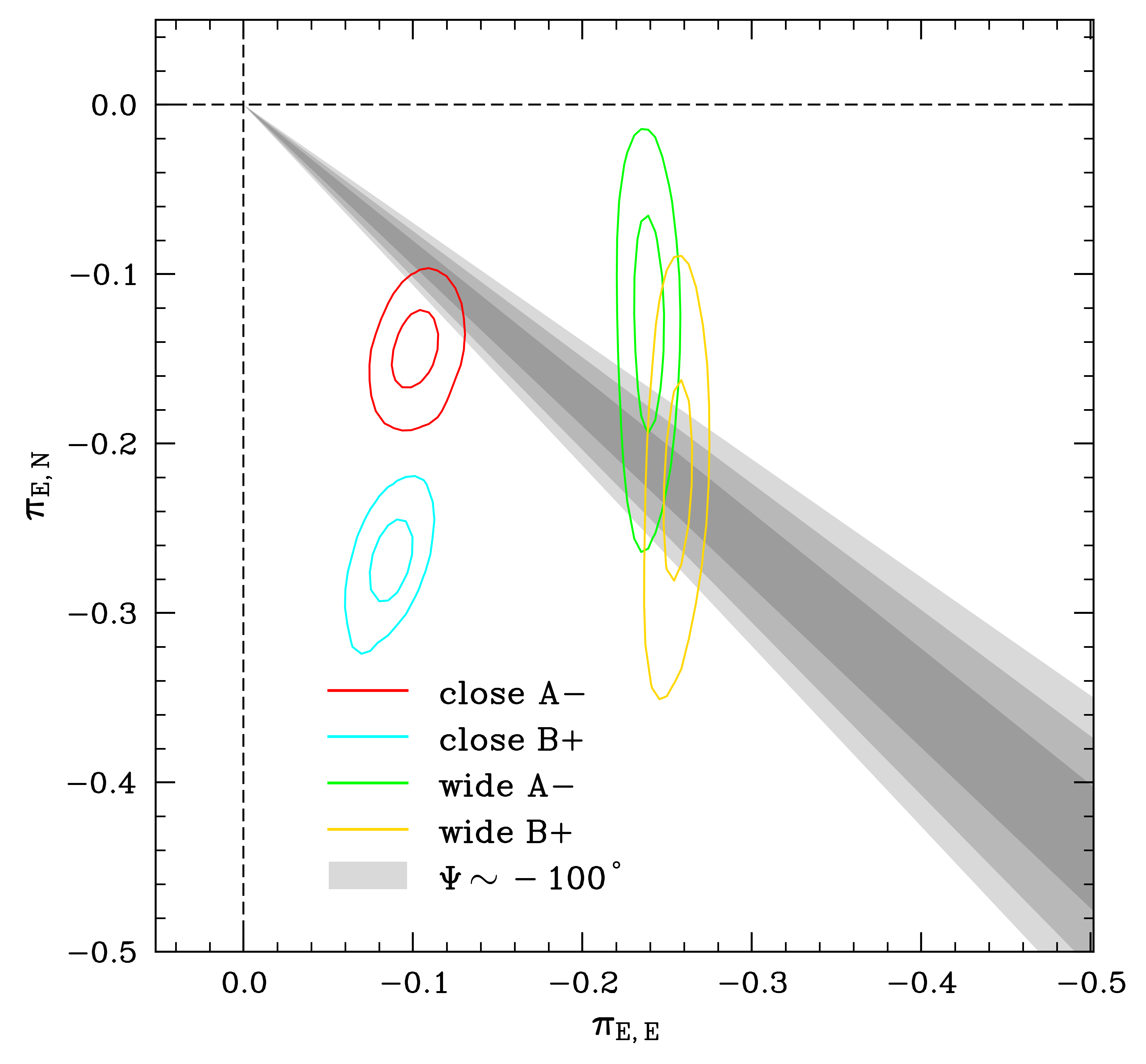
Figure 7: The 1 and 2$\sigma$ posterior distribution of the microlens parallax vector ${\bm{\pi}}_{\rm E}=(\pi_{{\rm E},{\rm E}},\pi_{{\rm E},{\rm N}})$ from light curve analysis for the “close A$+$” (red contours), “close B$+$” (cyan contours), “wide A$-$” (green contours) and “wide B$+$” (yellow contours) solutions, respectively. The shaded regions are the 1, 2, and 3$\sigma$ constraints on $\Phi_{\pi}$ derived from the interferometric data for the local minimum of $\Psi\sim-100^{\circ}$. The light-curve and VLTI constraints are consistent for the wide A$-$, wide B$+$ and close A$-$ solutions.

In this section, we present joint analysis of VLTI and light-curve modeling. We begin by comparing the light-curve parameters and VLTI constraints. Figure 6 shows the comparisons between the $\alpha$ parameters $\alpha_{\rm LC}$ derived from the light-curve solutions with $\alpha_{\rm VLTI}$. The three solutions are mutually compatible within $3\,\sigma$, and they are all at $\Psi\sim-100^{\circ}$. These include one close solution (“close A$-$”), and two wide solutions (“wide A$-$” and “wide B$+$”). Next we check the consistency of the direction ${\bm{\pi}}_{\rm E}$ between the light curve solutions and VLTI solution at $\Psi\sim-100^{\circ}$. Figure 7 displays the posterior distribution of $(\pi_{\rm E,E},\pi_{\rm E,N})$ and the $\Phi_{{\bm{\pi}}}$ constraint from VLTI. For three light-curve solutions (“wide A$-$”, “wide B$+$” and “close A$-$”), the two directions agree to $\sim 1\,\sigma$.

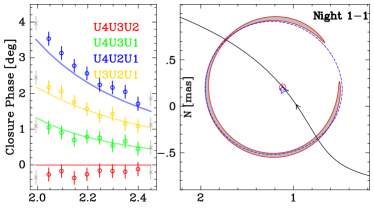
(a)

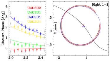
(b)

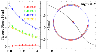
(c)

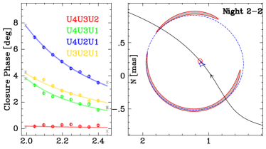
(d)

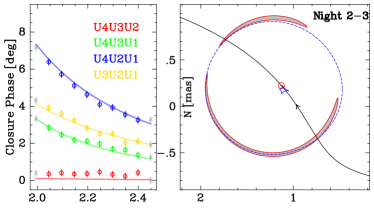
(e)

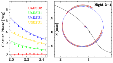
(f)

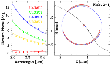
(g)

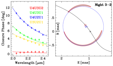
(h)

Figure 8: $4\times 2$ panel groups showing the closure phase data and the best-fit microlensing model (“wide A$-$”) for the eight VLTI GRAVITY exposures obtained over three nights. Within each group, the left sub-panel shows the closure phase data as a function of wavelength, with the best-fit model over-plotted as solid lines; the right sub-panel shows the caustics (blue), source trajectory (black line with an arrow) and source position (red circle) at the time of the VLTI observation, with the microlensed images displayed as shaded regions and the critical curves as blue dashed lines.

Then we perform a joint fit to the VLTI and light curve data for the “wide A$-$”, “wide B$+$” and “close A$-$” solutions. We include the higher-order effects of microlens parallax and binary orbital motion. Table 2 lists the best-fit parameters and their uncertainties. The global best-fit is the “wide A$-$” solution, and Figure 8 shows its best-fit closure-phase models along with the geometric configurations of the source, caustic and images. The “close A$-$” solution is worse by $\Delta\chi^{2}\approx 50$, which is somewhat ($\approx 15$) less compared with light-curve-only $\Delta\chi^{2}$. Therefore, the preference for the “wide A$-$” over the “close A$-$” comes from the light-curve fitting. It mainly stems from a $\sim 0.1$ mag broad bump-like feature in Gaia $G$-band light curve around $\rm HJD^{\prime}\sim 9300$, which can be only well matched by the wide solutions (see the right panel of Figure 4). In contrast, the “wide B$+$” model fit is worse by $\Delta\chi^{2}\approx 267$ with respect to “wide A$-$”, significantly increased by $\approx 218$ compared with light-curve only. As discussed in § 4.2, such $u_{0}>0$ geometries are strongly disfavored by the constraints from multi-epoch VLTI data.

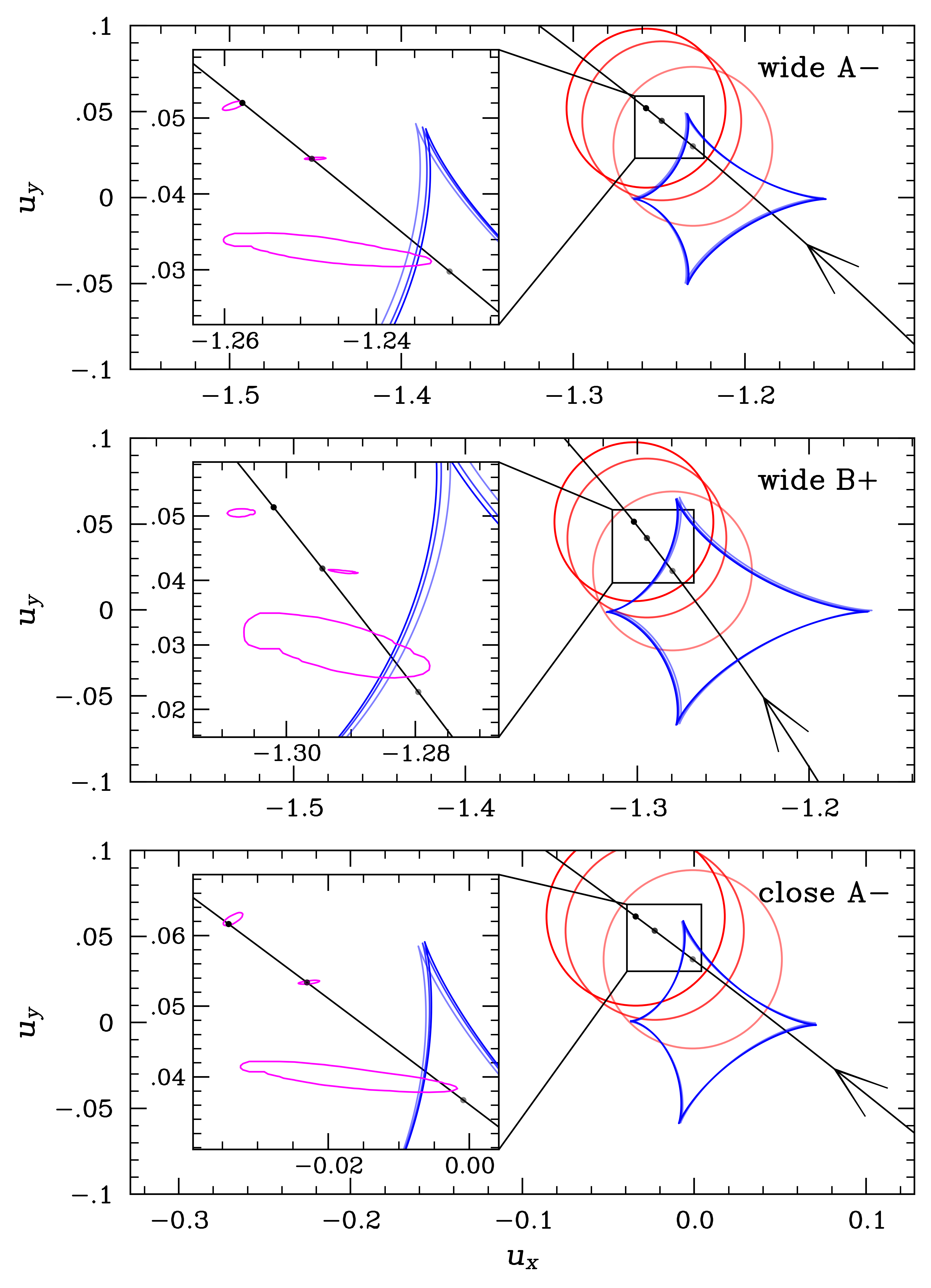
Figure 9: The source trajectory (black solid line) and caustics (blue closed curves) for “wide A$-$” (top panel), “wide B$+$” (middle panel) and “close A$-$” (bottom panel) solutions. The solid dots denote the source positions on the three nights of VLTI GRAVITY observations. The $3\sigma$ contours in magenta show the posteriors of the source positions inferred from the interferometric data only, with the geometric parameters $(s,q,\rho,\theta_{\rm E},\Psi)$ held fixed to the values in Table 2.

To further understand the VLTI constraints on these three solutions, we performed additional fitting with the interferometric data only. We hold the parameters $(s,q,\rho,\Psi,\theta_{\rm E})$, which define the caustics’ configuration, fixed at their best-fit values from the joint modeling, while the source positions $(u_{x},u_{y})$ of the three nights are allowed to vary. Figure 9 shows the $3\,\sigma$ $(u_{x},u_{y})$ contours (magenta) compared with the expected source positions (black dots) on the best-fit trajectory (black solid line) from the joint modeling for each solution. For the “wide A$-$” solution, there is a $\gtrsim 3\sigma$ discrepancy in $(u_{x},u_{y})$ during Night 1, which corresponds to the $\lesssim 0.3^{\circ}$ systematic residuals of the closure phases for U4U2U1 and U4U3U2 in both exposures of that night, as displayed in the top two sub-panels of Figure 8. During the other two nights, the source positions are in good agreements with the “wide A$-$” solution. Note that such $\sim 0.3^{\circ}$ systematic offsets also show up in the third exposure of Night 2 (see Figure 8), but they are not present in the other three exposures (i.e., Night 2-1, 2-2 and 2-4), which are in good agreement with the model. This suggests the existence of sub-degree level systematic error in the closure-phase data. The “close A$-$” solution shows a similar degree of consistency to the “wide A$-$”. In contrast, for the “wide B+” solution, which is ruled out by the VLTI data, the source positions of all three nights deviate by $>3\,\sigma$ from the expectation.

In conclusion, because the “wide A$-$” solution is preferred over all other local minima by $\Delta\chi^{2}\gtrsim 50$, we regard it as the only favored solution of ASASSN-22av.

5 Physical Parameters

5.1 Source Properties and Finite-Source Effects

The finite-source effects exhibited in ASASSN-22av’s light curves provide an opportunity to cross check the VLTI-measured $\theta_{\rm E}$ with $\theta_{\rm E}={\theta_{*}}/{\rho}$. The standard method (Yoo et al., 2004) to derive $\theta_{*}$ for bulge microlensing events uses the source’s de-reddened color and magnitude with the extinction coefficients estimated from the location of bulge red clump (RC) stars in a color-magnitude diagram (CMD). In our case, the source star is not toward the bulge, and the CMD contains RC stars at a variety of distances, making it difficult to apply the standard method. Gaia DR3 reports a trigonometric parallax $\pi_{\rm S}=0.137\pm 0.016\,{\rm mas}$. We adopt $\pi_{{\rm S},\rm corr}=0.185\,{\rm mas}$ after applying the preliminary zero-point correction from Lindegren et al. (2021). The independent investigation on the Gaia parallax zero-point offset by Groenewegen (2021) yields a consistent value of $\pi_{{\rm S},\rm corr}=0.207\pm 0.025\,{\rm mas}$. We fit the spectral energy distribution (SED) using photometric data from 2MASS, Gaia and SkyMapper Southern Survey Data Release 4 (SMSS DR4; Onken et al., 2024). We employ the MESA Isochrones and Stellar Tracks (MIST; Choi et al., 2016) to generate synthetic magnitudes as a function of stellar mass, age, and metallicity. The extinction $E(B-V)$ is taken as a free parameter with a flat prior, and we assume that $R_{V}=3.1$. We use the corrected Gaia parallax as a prior for source distance. MIST returns the stellar radius $R_{*}$, and hence, the angular radius $\theta_{*}=R_{*}/D_{\rm S}$ can be estimated with MCMC. The photometric error bars are inflated by a factor of 2 so that $\chi^{2}/{\rm d.o.f}\sim 1$. We find that the best-fit $E(B-V)=0.64^{+0.06}_{-0.04}$, which is consistent with the lower limit of $E(B-V)>0.61$ (for distance greater than $4.3$ kpc) according to the 3D dust map of Guo et al. (2021). The best-fit stellar parameters are $T_{\rm eff}=3747^{+46}_{-18}\,{\rm K},\,\log g=1.07^{+0.11}_{-0.04}$ and $[{\rm Fe/H}]=0.01^{+0.12}_{-0.07}$, arriving at $\theta_{*}=44.0\pm 0.8\,\mu\rm as$. The SED-derived stellar parameters are consistent with the spectroscopic ones from § 2.3.

For the best-fit “wide A$-$” solution with $\rho=0.059\pm 0.001$, we find $\theta_{\rm E}=0.746\pm 0.019\,{\rm mas}$, which differs by $1\sigma$ from the $\theta_{\rm E}=0.726\pm 0.002\,{\rm mas}$ determined by VLTI GRAVITY. In comparison, for the “close A$-$” solution, where $\rho=0.052^{+0.001}_{-0.001}$, the corresponding $\theta_{\rm E}=0.846\pm 0.022\,{\rm mas}$ deviates from the VLTI GRAVITY value of $\theta_{\rm E}\simeq 0.736\pm 0.002\,{\rm mas}$ by $5\sigma$. Note that the $\sim 2\,\%$ error of our $\theta_{*}$ estimate is likely an underestimate due to unaccounted systematic uncertainties. For example, $\theta_{*}$ inferences from the empirical color/surface-brightness relations such as Kervella et al. (2004) generally have errors of $\sim 4$–$5\,\%$. In any case, for the “wide A$-$” solution, $\theta_{\rm E}$ derived from VLTI and finite-source effects are consistent.

5.2 Physical Properties of the Lens System

With measurements of the angular Einstein radius $\theta_{\rm E}$ and the microlens parallax $\pi_{\rm E}$, the physical parameters of the lens system can be unambiguously derived from microlensing observables:

$$M_{\rm L}=\frac{\theta_{\rm E}}{\kappa\pi_{\rm E}};\quad\pi_{\rm rel}=\theta_{\rm E}\pi_{\rm E};\quad{\bm{\mu}}_{\rm rel}=\frac{\theta_{\rm E}}{t_{\rm E}}\,\frac{{\bm{\pi}}_{\rm E}}{\pi_{\rm E}},$$ (11)

and adopting $\pi_{\rm S}=0.185\pm 0.016\,{\rm mas}$, we can also infer the lens distance,

$$D_{\rm L}=\frac{{\rm AU}}{\pi_{\rm E}\theta_{\rm E}+\pi_{\rm S}}.$$ (12)

The lens properties of the favored solution (“wide A$-$”) are listed in Table 3. The lens system is composed of two M dwarfs with $M_{1}=0.261^{+0.009}_{-0.008}\,M_{\odot}$ and $M_{2}=0.252\pm{0.017}\,M_{\odot}$, separated by a projected separation of $r_{\perp}=7.42\pm 0.33\,{\rm AU}$, and at a distance of $D_{\rm L}=2.31\pm 0.09$ kpc.

Based on MIST isochrones, we estimate that the lens system has $K_{s}=18.5$ (assuming zero extinction). In comparison, the source’s 2MASS magnitude is $K_{s}=9.23$. During the VLTI observations, the magnification is more than $15$, and thus the flux ratio between the lens and magnified source is $\xi=f_{{\rm L}}/(Af_{{\rm S}})<1.4\times 10^{-5}$. Therefore, the lens light has a negligible effect on the closure phase, justifying our approach of calculating closure phases without the lens flux contribution.

6 Discussion and Conclusion

ASASSN-22av is the first binary-lens microlensing event with multiple images resolved by interferometry. The modeling is considerably more complex than for a single-lens event. For a typical single-lens event, the simple model of two point images is generally satisfactory for fitting the closure-phase data (Dong et al., 2019), and thus, closure-phase modeling can, in principle, be performed separately from the light curve. In contrast, a binary lens has three or five images for a point source, depending on whether the source is outside or inside the caustics. During the VLTI observations of ASASSN-22av, the images, formed from a finite source crossing caustics, morphed from a nearly complete Einstein ring to separated arcs over a period of several nights. Thus, the interpretation of the closure-phase data from such a binary-lens event requires inputs from light-curve modeling.

The weak binary perturbation and sparse pre-peak photometric coverage make the light-curve modeling particularly complicated for ASASSN-22av. In the early stages of our work where we did not include the Gaia light curve, we found 25 local minima in our binary-lens grid search. After incorporating the VLTI data, the best-fit solution, which is the same as the presently-favored “wide A$-$” solution, ‘predicted’ the existence of the bump at $\rm HJD^{\prime}\sim 9300$ shown in the Gaia light curve. We only realized this ‘prediction’ later, after conducting light-curve modeling after the inclusion of Gaia data. The predictive power of the “wide A$-$” solution offers good evidence for its validity.

We also made several consistency checks between the light curve and multi-epoch VLTI data. For the favored solution, there are good agreements in multiple aspects, including $\alpha$ (Figure 6), direction of ${\bm{\pi}}_{\rm E}$ (Figure 7), source trajectory (Figure 9) and $\theta_{\rm E}$ (see discussion in § 5.1), further demonstrating the model’s robustness. The agreement between the best-fit model and the closure-phase data is at $\lesssim 0.3^{\circ}$ (Figure 8, §4.3), which likely reflects the instrument’s systematics floor. We measure the Einstein radius $\theta_{\rm E}=0.726$ mas with $0.3\%$ precision, even thought it is close to the smallest value resolvable by VLTI GRAVITY. The expected closure phase would be $\lesssim 5^{\circ}$ for $\theta_{\rm E}$ to $0.6\,{\rm mas}$ and $\lesssim 2^{\circ}$ for $\theta_{\rm E}=0.5\,{\rm mas}$.

The lens system consists of two M dwarfs separated by $\sim 7.4\,{\rm AU}$ at $2.3\,\rm kpc$, with $(M_{1},M_{2})=(0.261\pm{0.009},0.252\pm{0.017})\,M_{\sun}$. The primary mass is more precisely determined than the secondary ($3.4\%$ versus $6.7\%$). This is because, in the wide-binary ($s>1$) regime, the scale of images (measured by VLTI GRAVITY) is proportional to $\theta_{\rm E}$ of the primary mass rather than the total mass. Hence, the uncertainty of the secondary mass $M_{2}$ is contributed by an additional uncertainty from the mass ratio. The estimated orbital period is $P\sim 27\,\rm yr$ for a circular orbit, and the angular separation between the binaries is $\sim 3\,{\rm mas}$ at $2.3\,\rm kpc$. Such faint low-mass binary systems at intermediate separations have so far been inaccessible by any other method (El-Badry, 2024, see their Figure 1). Similar VLTI microlensing observations will be able to identify and characterize intermediate binaries containing dark compact objects like neutron stars and stellar-mass black holes to complement other detection techniques.

Appendix A Binning the closure-phase data

The interferometric observables are the complex visibilities $\mathcal{V}_{pq}$ and closure phases $\phi_{pqr}$, with (van Cittert, 1934; Zernike, 1938)

$$\mathcal{V}_{pq}(u,v;\lambda)=\frac{\int I(\alpha,\delta)e^{-2\pi i(u\alpha+v\delta)}d\alpha d\delta}{\int I(\alpha,\delta)d\alpha d\delta},$$ (A1)

where $I(\alpha,\delta)$ is the on-sky target intensity distribution centered on light of sight $(\alpha_{0},\delta_{0})$, and $(u,v)=(\bm{n}_{\rm E},\bm{n}_{\rm N})\cdot\bm{B}_{pq}/\lambda$ is the on-sky projection of baseline vector over wavelength. The closure phase is defined for a three telescope array as $\phi_{pqr}(\lambda)=\arg(\mathcal{V}_{pq}\mathcal{V}_{qr}\mathcal{V}_{rp})$. For a list of closure phases $\{\phi_{k}\}$, the mean closure phase $\bar{\phi}$ is calculated by assigning $\phi_{k}$ to unit complex and summing them up for binning as

$$\bar{\phi}=\arg\sum_{k}e^{i\phi_{k}}.$$ (A2)

The uncertainty of $\bar{\phi}$ is estimated using bootstrap resampling.

Appendix B image generation and visibility calculation

For given source coordinate $(u_{x},u_{y})$ and binary configuration $(s,q)$, we extract the image contours used for the magnification calculation in VBBinaryLensing package. The contours are then converted to 2D images using the loop-linking method (Dong et al., 2006), which combines the contour integration and inverse ray-shooting methods. The loop-linking method fills the contour with a uniform grid of points organized in vertical links of points. Our code returns the head $(x_{k},y_{k})$, the length $n_{k}$ of every link, and the spacing of the mesh grid $\delta$. For any baseline coordinate $(u,v)$, the complex visibility is calculated by summing up the contribution from all links (assuming $\Psi=0$) as

$$\mathcal{V}(u,v) =\sum_{k}\sum_{j=0}^{n_{k}-1}e^{-2\pi i(vx_{k}+u(y_{k}+j\delta))}$$

$$=\sum_{k}e^{-2\pi i(vx_{k}+uy_{k})}\sum_{j=0}^{n_{k}-1}(e^{-2\pi iu\delta})^{j}$$

$$=\sum_{k}e^{-2\pi i(vx_{k}+uy_{k})}\frac{1-e^{-2\pi iu\delta n_{k}}}{1-e^{-2\pi iu\delta}}.$$

The calculation is optimized by grouping the links by $n_{k}$ and summing up them first, which reduces the number of calculations by a factor of $\sim 2$. We caution that the dot product of $(x_{k},y_{k})$ and $(u,v)$ is not arbitrary. In our case, it has to be $x_{k}v+y_{k}u$. Otherwise, the transformation from the image plane to the sky plane is not positive-definite and the angle $\Psi$ is not well-defined.

An alternative method to compute the visibility is applying the divergence theorem on the closed image contour $\partial D$ with

$$V(\bm{u})=\iint_{D}e^{-2\pi i\bm{u}\cdot\bm{r}}d^{2}\bm{r}=\oint_{\partial D}e^{-2\pi i\bm{u}\cdot\bm{r}}\frac{\bm{u}\cdot\bm{\hat{n}}}{-2\pi iu^{2}}ds,$$ (B1)

where $\bm{\hat{n}}$ the unit vector normal to the boundary $\partial D$ at $\bm{r}$. For a closed polygon with vertices $\bm{r}_{k}$, the integration for edge $\bm{r}_{k}\to\bm{r}_{k+1}$ is

$$\int_{\bm{r}_{k}}^{\bm{r}_{k+1}}e^{-2\pi i\bm{u}\cdot\bm{r}}\frac{\bm{u}\times d\bm{r}}{-2\pi iu^{2}}=\frac{1}{4\pi^{2}u^{2}}\frac{\bm{u}\times(\bm{r}_{k}-\bm{r}_{k+1})}{\bm{u}\cdot(\bm{r}_{k}-\bm{r}_{k+1})}(e^{-2\pi i\bm{u}\cdot\bm{r}_{k}}-e^{-2\pi i\bm{u}\cdot\bm{r}_{k+1}}).$$ (B2)

The visibility is then the sum over all edges. This method is faster than the loop-linking method for convex images, while the loop-linking method is faster for concave images. In our case, the images are ring-like arcs, and thus we adopt the loop-linking method.

Table 1: Best-fit light-curve parameters and $1\sigma$ uncertainties

Solution	$t_{0}$	$u_{0}$	$t_{\mathrm{E}}$	$\rho$	$s$	$q$	$\alpha$	$\pi_{\rm E,N}$	$\pi_{\rm E,E}$	$ds/dt$	$d\alpha/dt$	$\beta$
$\chi^{2}$	$\rm HJD^{\prime}$		$\rm day$				$\rm deg$			$\rm yr^{-1}$	$\rm yr^{-1}$
close A$+$	$9601.24$	$0.035$	$65.4$	$0.056$	$0.4$	$0.36$	$37.4$	$-0.28$	$-0.14$	$0.15$	$-1.41$	$0.03$
1005.3	${}^{+0.04}_{-0.05}$	${}^{+0.002}_{-0.002}$	${}^{+1.3}_{-1.1}$	${}^{+0.002}_{-0.002}$	${}^{+0.1}_{-0.1}$	${}^{+0.04}_{-0.03}$	${}^{+0.6}_{-0.6}$	${}^{+0.04}_{-0.03}$	${}^{+0.02}_{-0.02}$	${}^{+0.02}_{-0.02}$	${}^{+0.07}_{-0.06}$	${}^{+0.01}_{-0.01}$
close A$-$	$9601.11$	$-0.028$	$74.0$	$0.048$	$0.4$	$0.21$	$-38.1$	$-0.14$	$-0.10$	$0.20$	$2.11$	$0.12$
1013.5	${}^{+0.06}_{-0.04}$	${}^{+0.002}_{-0.002}$	${}^{+1.4}_{-1.8}$	${}^{+0.003}_{-0.002}$	${}^{+0.1}_{-0.1}$	${}^{+0.04}_{-0.02}$	${}^{+0.6}_{-0.6}$	${}^{+0.03}_{-0.03}$	${}^{+0.02}_{-0.02}$	${}^{+0.02}_{-0.03}$	${}^{+0.05}_{-0.08}$	${}^{+0.02}_{-0.03}$
close B$+$	$9601.35$	$0.040$	$63.5$	$0.056$	$0.4$	$0.50$	$-47.9$	$-0.27$	$-0.09$	$0.16$	$1.49$	$0.03$
1025.9	${}^{+0.03}_{-0.03}$	${}^{+0.002}_{-0.002}$	${}^{+0.9}_{-1.1}$	${}^{+0.002}_{-0.002}$	${}^{+0.1}_{-0.1}$	${}^{+0.05}_{-0.05}$	${}^{+0.5}_{-0.5}$	${}^{+0.03}_{-0.02}$	${}^{+0.02}_{-0.02}$	${}^{+0.01}_{-0.01}$	${}^{+0.06}_{-0.06}$	${}^{+0.01}_{-0.01}$
wide A$+$	$9601.34$	$0.035$	$56.3$	$0.068$	$5.4$	$1.04$	$33.2$	$-0.40$	$-0.03$	$0.80$	$0.16$	$0.98$
1028.4	${}^{+0.03}_{-0.04}$	${}^{+0.002}_{-0.002}$	${}^{+1.4}_{-1.3}$	${}^{+0.002}_{-0.003}$	${}^{+0.2}_{-0.2}$	${}^{+0.08}_{-0.07}$	${}^{+0.6}_{-0.5}$	${}^{+0.03}_{-0.03}$	${}^{+0.02}_{-0.02}$	${}^{+0.14}_{-0.15}$	${}^{+0.03}_{-0.04}$	${}^{+0.02}_{-0.05}$
wide A$-$	$\bf 9601.30$	$\bf-0.028$	$\bf 69.5$	$\bf 0.054$	$\bf 5.1$	$\bf 0.77$	$\bf-38.5$	$\bf-0.13$	$\bf-0.24$	$\bf 0.19$	$\bf-0.11$	$\bf 0.39$
948.9	${}^{+0.08}_{-0.07}$	${}^{+0.002}_{-0.002}$	${}^{+3.0}_{-3.3}$	${}^{+0.002}_{-0.002}$	${}^{+0.3}_{-0.3}$	${}^{+0.09}_{-0.08}$	${}^{+1.1}_{-0.9}$	${}^{+0.06}_{-0.08}$	${}^{+0.02}_{-0.01}$	${}^{+0.34}_{-0.33}$	${}^{+0.06}_{-0.05}$	${}^{+0.31}_{-0.18}$
wide B$+$	$9601.07$	$0.033$	$61.1$	$0.054$	$6.2$	$1.27$	$-39.0$	$-0.22$	$-0.26$	$1.03$	$-0.00$	$0.87$
999.6	${}^{+0.04}_{-0.04}$	${}^{+0.002}_{-0.002}$	${}^{+1.9}_{-1.9}$	${}^{+0.003}_{-0.002}$	${}^{+0.3}_{-0.3}$	${}^{+0.12}_{-0.09}$	${}^{+1.1}_{-1.1}$	${}^{+0.07}_{-0.07}$	${}^{+0.01}_{-0.01}$	${}^{+0.07}_{-0.14}$	${}^{+0.04}_{-0.03}$	${}^{+0.07}_{-0.20}$

Table 2: Best-fit parameters and $1\sigma$ uncertainties from the joint VLTI and light-curve analysis

Solution	$t_{0}$	$u_{0}$	$t_{\mathrm{E}}$	$\rho$	$s$	$q$	$\alpha$	$\pi_{\rm E}$	$ds/dt$	$d\alpha/dt$	$\beta$	$\theta_{\rm E}$	$\Psi$
$\chi^{2}$	$\rm HJD^{\prime}$		$\rm day$				$\rm deg$		$\rm yr^{-1}$	$\rm yr^{-1}$		${\rm mas}$	$\rm deg$
close A$-$	$9601.16$	$-0.029$	$72.7$	$0.052$	$0.4$	$0.26$	$-37.3$	$0.18$	$0.18$	$2.04$	$0.09$	$0.736$	$259.9$
1227.3	${}^{+0.02}_{-0.02}$	${}^{+0.001}_{-0.001}$	${}^{+0.7}_{-0.8}$	${}^{+0.001}_{-0.001}$	${}^{+0.1}_{-0.1}$	${}^{+0.01}_{-0.01}$	${}^{+0.4}_{-0.4}$	${}^{+0.01}_{-0.01}$	${}^{+0.01}_{-0.01}$	${}^{+0.02}_{-0.03}$	${}^{+0.01}_{-0.01}$	${}^{+0.002}_{-0.002}$	${}^{+0.2}_{-0.2}$
wide A$-$	$\bf 9601.14$	$\bf-0.029$	$\bf 68.3$	$\bf 0.059$	$\bf 4.4$	$\bf 0.60$	$\bf-39.8$	$\bf 0.34$	$\bf-0.54$	$\bf-0.07$	$\bf 0.26$	$\bf 0.726$	$\bf 260.8$
1177.8	${}^{+0.03}_{-0.04}$	${}^{+0.001}_{-0.001}$	${}^{+1.0}_{-1.1}$	${}^{+0.001}_{-0.001}$	${}^{+0.1}_{-0.1}$	${}^{+0.03}_{-0.03}$	${}^{+0.5}_{-0.5}$	${}^{+0.01}_{-0.02}$	${}^{+0.21}_{-0.18}$	${}^{+0.03}_{-0.02}$	${}^{+0.20}_{-0.12}$	${}^{+0.002}_{-0.002}$	${}^{+0.2}_{-0.3}$
wide B$+$	$9600.68$	$-0.005$	$62.5$	$0.062$	$4.3$	$0.81$	$-52.9$	$0.48$	$0.73$	$-0.09$	$0.27$	$0.728$	$263.2$
1477.6	${}^{+0.02}_{-0.02}$	${}^{+0.001}_{-0.001}$	${}^{+0.6}_{-0.5}$	${}^{+0.001}_{-0.001}$	${}^{+0.1}_{-0.1}$	${}^{+0.03}_{-0.03}$	${}^{+0.3}_{-0.2}$	${}^{+0.01}_{-0.01}$	${}^{+0.04}_{-0.03}$	${}^{+0.02}_{-0.02}$	${}^{+0.03}_{-0.04}$	${}^{+0.002}_{-0.002}$	${}^{+0.1}_{-0.2}$

Table 3: Derived physical parameters of the lens system

$M_{1}$	$M_{2}$	$r_{\perp}$	$\pi_{\rm rel}$	$D_{\rm L}$	$\mu_{\rm hel,N}$	$\mu_{\rm hel,E}$
$M_{\sun}$	$M_{\sun}$	${\rm AU}$	${\rm mas}$	$\rm kpc$	$\rm mas\,yr^{-1}$	$\rm mas\,yr^{-1}$
$0.261^{+0.009}_{-0.008}$	$0.252^{+0.017}_{-0.017}$	$7.42^{+0.33}_{-0.33}$	$0.248^{+0.007}_{-0.008}$	$2.31^{+0.09}_{-0.09}$	$-1.40^{+0.06}_{-0.05}$	$-2.80^{+0.05}_{-0.06}$

References

- Afonso et al. (2001) Afonso, C., Albert, J. N., Andersen, J., et al. 2001, A&A, 378, 1014. doi:10.1051/0004-6361:20011204
- Alard & Lupton (1998) Alard, C. & Lupton, R. H. 1998, ApJ, 503, 325. doi:10.1086/305984
- Alard (2000) Alard, C. 2000, A&AS, 144, 363. doi:10.1051/aas:2000214
- Albrow et al. (2001) Albrow, M., An, J., Beaulieu, J.-P., et al. 2001, ApJ, 550, L173. doi:10.1086/319635
- An et al. (2002) An, J. H., Albrow, M. D., Beaulieu, J.-P., et al. 2002, ApJ, 572, 521. doi:10.1086/340191
- Batista et al. (2011) Batista, V., Gould, A., Dieters, S., et al. 2011, A&A, 529, A102. doi:10.1051/0004-6361/201016111
- Becker (2015) Becker, A. 2015, Astrophysics Source Code Library. ascl:1504.004
- Bernstein et al. (2003) Bernstein, R., Shectman, S. A., Gunnels, S. M., et al. 2003, Proc. SPIE, 4841, 1694. doi:10.1117/12.461502
- Bozza (2010) Bozza, V. 2010, MNRAS, 408, 2188. doi:10.1111/j.1365-2966.2010.17265.x
- Bozza et al. (2018) Bozza, V., Bachelet, E., Bartolić, F., et al. 2018, MNRAS, 479, 5157. doi:10.1093/mnras/sty1791
- Brown et al. (2013) Brown, T. M., Baliber, N., Bianco, F. B., et al. 2013, PASP, 125, 1031. doi:10.1086/673168
- Buckley et al. (2006) Buckley, D. A. H., Swart, G. P., & Meiring, J. G. 2006, Proc. SPIE, 6267, 62670Z. doi:10.1117/12.673750
- Buder et al. (2018) Buder, S., Asplund, M., Duong, L., et al. 2018, MNRAS, 478, 4513. doi:10.1093/mnras/sty1281
- Buder et al. (2019) Buder, S., Lind, K., Ness, M. K., et al. 2019, A&A, 624, A19. doi:10.1051/0004-6361/201833218
- Buder et al. (2021) Buder, S., Sharma, S., Kos, J., et al. 2021, MNRAS, 506, 150. doi:10.1093/mnras/stab1242
- Cassan & Ranc (2016) Cassan, A., & Ranc, C. 2016, MNRAS, 458, 2074
- Cassan et al. (2022) Cassan, A., Ranc, C., Absil, O., et al. 2022, Nature Astronomy, 6, 121. doi:10.1038/s41550-021-01514-w
- Chang & Refsdal (1979) Chang, K. & Refsdal, S. 1979, Nature, 282, 561. doi:10.1038/282561a0
- Chen et al. (2022) Chen, P., Dong, S., Kochanek, C. S., et al. 2022, ApJS, 259, 53. doi:10.3847/1538-4365/ac50b7
- Choi et al. (2016) Choi, J., Dotter, A., Conroy, C., et al. 2016, ApJ, 823, 102. doi:10.3847/0004-637X/823/2/102
- Claret & Bloemen (2011) Claret, A. & Bloemen, S. 2011, A&A, 529, A75. doi:10.1051/0004-6361/201116451
- Claret (2019) Claret, A. 2019, VizieR Online Data Catalog, 6154. VI/154
- Dalal & Lane (2003) Dalal, N., & Lane, B. F. 2003, ApJ, 589, 199
- Delplancke et al. (2001) Delplancke, F., Górski, K. M., & Richichi, A. 2001, A&A, 375, 701
- De Silva et al. (2015) De Silva, G. M., Freeman, K. C., Bland-Hawthorn, J., et al. 2015, MNRAS, 449, 2604. doi:10.1093/mnras/stv327
- Dong et al. (2006) Dong, S., DePoy, D. L., Gaudi, B. S., et al. 2006, ApJ, 642, 842. doi:10.1086/501224
- Dong et al. (2007) Dong, S., Udalski, A., Gould, A., et al. 2007, ApJ, 664, 862. doi:10.1086/518536
- Dong et al. (2009) Dong, S., Gould, A., Udalski, A., et al. 2009, ApJ, 695, 970. doi:10.1088/0004-637X/695/2/970
- Dong et al. (2019) Dong, S., Mérand, A., Delplancke-Ströbele, F., et al. 2019, ApJ, 871, 70. doi:10.3847/1538-4357/aaeffb
- Einstein (1936) Einstein, A. 1936, Science, 84, 506. doi:10.1126/science.84.2188.506
- Eisenhauer et al. (2023) Eisenhauer, F., Monnier, J. D., & Pfuhl, O. 2023, ARA&A, 61, 237. doi:10.1146/annurev-astro-121622-045019
- El-Badry (2024) El-Badry, K. 2024, New A Rev., 98, 101694. doi:10.1016/j.newar.2024.101694
- Foreman-Mackey et al. (2013) Foreman-Mackey, D., Hogg, D. W., Lang, D., et al. 2013, PASP, 125, 306. doi:10.1086/670067
- Gaia Collaboration et al. (2016) Gaia Collaboration, Prusti, T., de Bruijne, J. H. J., et al. 2016, A&A, 595, A1. doi:10.1051/0004-6361/201629272
- Gaia Collaboration et al. (2023) Gaia Collaboration, Vallenari, A., Brown, A. G. A., et al. 2023, A&A, 674, A1. doi:10.1051/0004-6361/202243940
- Gould (1992) Gould, A. 1992, ApJ, 392, 442. doi:10.1086/171443
- Gould (1994a) Gould, A. 1994, ApJ, 421, L71. doi:10.1086/187190
- Gould (1994b) Gould, A. 1994, ApJ, 421, L75. doi:10.1086/187191
- Gould et al. (1994) Gould, A., Miralda-Escude, J., & Bahcall, J. N. 1994, ApJ, 423, L105. doi:10.1086/187247
- Gould (2000) Gould, A. 2000, ApJ, 542, 785
- Gould (2004) Gould, A. 2004, ApJ, 606, 319. doi:10.1086/382782
- GRAVITY Collaboration et al. (2017) GRAVITY Collaboration, Abuter, R., Accardo, M., et al. 2017, A&A, 602, A94. doi:10.1051/0004-6361/201730838
- GRAVITY+ Collaboration et al. (2022a) GRAVITY+ Collaboration, Abuter, R., Allouche, F., et al. 2022, A&A, 665, A75. doi:10.1051/0004-6361/202243941
- GRAVITY+ Collaboration et al. (2022b) GRAVITY+ Collaboration, Abuter, R., Alarcon, P., et al. 2022, The Messenger, 189, 17. doi:10.18727/0722-6691/5285
- Groenewegen (2021) Groenewegen, M. A. T. 2021, A&A, 654, A20. doi:10.1051/0004-6361/202140862
- Guo et al. (2021) Guo, H.-L., Chen, B.-Q., Yuan, H.-B., et al. 2021, ApJ, 906, 47. doi:10.3847/1538-4357/abc68a
- Hodgkin et al. (2021) Hodgkin, S. T., Harrison, D. L., Breedt, E., et al. 2021, A&A, 652, A76. doi:10.1051/0004-6361/202140735
- Jung et al. (2022) Jung, Y. K., Zang, W., Han, C., et al. 2022, AJ, 164, 262. doi:10.3847/1538-3881/ac9c5c
- Kammerer et al. (2020) Kammerer, J., Mérand, A., Ireland, M. J., et al. 2020, A&A, 644, A110. doi:10.1051/0004-6361/202038563
- Kervella et al. (2004) Kervella, P., Bersier, D., Mourard, D., et al. 2004, A&A, 428, 587
- Kochanek et al. (2017) Kochanek, C. S., Shappee, B. J., Stanek, K. Z., et al. 2017, PASP, 129, 104502. doi:10.1088/1538-3873/aa80d9
- Kos et al. (2017) Kos, J., Lin, J., Zwitter, T., et al. 2017, MNRAS, 464, 1259. doi:10.1093/mnras/stw2064
- Le Bouquin et al. (2011) Le Bouquin, J.-B., Berger, J.-P., Lazareff, B., et al. 2011, A&A, 535, A67. doi:10.1051/0004-6361/201117586
- Lindegren et al. (2021) Lindegren, L., Bastian, U., Biermann, M., et al. 2021, A&A, 649, A4. doi:10.1051/0004-6361/202039653
- Lindegren et al. (2021) Lindegren, L., Klioner, S. A., Hernández, J., et al. 2021, A&A, 649, A2. doi:10.1051/0004-6361/202039709
- Mayor et al. (2003) Mayor, M., Pepe, F., Queloz, D., et al. 2003, The Messenger, 114, 20
- Mérand (2022) Mérand, A. 2022, Proc. SPIE, 12183, 121831N. doi:10.1117/12.2626700
- Mróz et al. (2024) Mróz, P., Dong, S., Mérand, A., et al. 2024, Submitted
- Onken et al. (2024) Onken, C. A., Wolf, C., Bessell, M. S., et al. 2024, arXiv:2402.02015. doi:10.48550/arXiv.2402.02015
- Paczyński (1986) Paczyński, B. 1986, ApJ, 304, 1. doi:10.1086/164140
- Piskunov & Valenti (2017) Piskunov, N. & Valenti, J. A. 2017, A&A, 597, A16. doi:10.1051/0004-6361/201629124
- Rattenbury & Mao (2006) Rattenbury, N. J., & Mao, S. 2006, MNRAS, 365, 792
- Recio-Blanco et al. (2023) Recio-Blanco, A., de Laverny, P., Palicio, P. A., et al. 2023, A&A, 674, A29. doi:10.1051/0004-6361/202243750
- Refsdal (1966) refsdal, s. 1966, MNRAS, 134, 315
- Riello et al. (2021) Riello, M., De Angeli, F., Evans, D. W., et al. 2021, A&A, 649, A3. doi:10.1051/0004-6361/202039587
- Rybicki et al. (2022) Rybicki, K. A., Wyrzykowski, L., Bachelet, E., et al. 2022, A&A, 657, A18. doi:10.1051/0004-6361/202039542
- Schechter et al. (1993) Schechter, P. L., Mateo, M., & Saha, A. 1993, PASP, 105, 1342. doi:10.1086/133316
- Shappee et al. (2014) Shappee, B. J., Prieto, J. L., Grupe, D., et al. 2014, ApJ, 788, 48. doi:10.1088/0004-637X/788/1/48
- Sheinis et al. (2015) Sheinis, A., Anguiano, B., Asplund, M., et al. 2015, Journal of Astronomical Telescopes, Instruments, and Systems, 1, 035002. doi:10.1117/1.JATIS.1.3.035002
- Skowron et al. (2011) Skowron, J., Udalski, A., Gould, A., et al. 2011, ApJ, 738, 87. doi:10.1088/0004-637X/738/1/87
- Skrutskie et al. (2006) Skrutskie, M. F., Cutri, R. M., Stiening, R., et al. 2006, AJ, 131, 1163. doi:10.1086/498708
- Smith et al. (2003) Smith, M. C., Mao, S., & Paczyński, B. 2003, MNRAS, 339, 925. doi:10.1046/j.1365-8711.2003.06183.x
- Ting et al. (2019) Ting, Y.-S., Conroy, C., Rix, H.-W., et al. 2019, ApJ, 879, 69. doi:10.3847/1538-4357/ab2331
- Yee et al. (2012) Yee, J. C., Shvartzvald, Y., Gal-Yam, A., et al. 2012, ApJ, 755, 102. doi:10.1088/0004-637X/755/2/102
- Yoo et al. (2004) Yoo, J., DePoy, D. L., Gal-Yam, A., et al. 2004, ApJ, 603, 139. doi:10.1086/381241
- van Cittert (1934) van Cittert, P. H. 1934, Physica, 1, 201. doi:10.1016/S0031-8914(34)90026-4
- Wyrzykowski et al. (2023) Wyrzykowski, L., Kruszyńska, K., Rybicki, K. A., et al. 2023, A&A, 674, A23. doi:10.1051/0004-6361/202243756
- Zang et al. (2020) Zang, W., Dong, S., Gould, A., et al. 2020, ApJ, 897, 180. doi:10.3847/1538-4357/ab9749
- Zernike (1938) Zernike, F. 1938, Physica, 5, 785. doi:10.1016/S0031-8914(38)80203-2
- Zhu et al. (2014) Zhu, W., Penny, M., Mao, S., et al. 2014, ApJ, 788, 73. doi:10.1088/0004-637X/788/1/73