HOD-informed prior for EFT-based full-shape analyses of LSS

Abstract

To improve the performance of full-shape analyses of large-scale structure, we consider using a halo occupation distribution (HOD)-informed prior for the effective field theory (EFT) nuisance parameters. We generate 320 000 mock galaxy catalogs using 10 000 sets of HOD parameters across 32 simulation boxes with different cosmologies. We measure and fit the redshift-space power spectra using a fast emulator of the EFT model, and the resulting best-fit EFT parameter distributions are used to create the prior. This prior effectively constrains the EFT nuisance parameter space, limiting it to the space of HOD-mocks that can be well fit by a EFT model. We have tested the stability of the prior under different configurations, including the effect of varying the HOD sample distribution and the inclusion of the hexadecapole moment. We find that our HOD-informed prior and the cosmological parameter constraints derived using it are robust. While cosmological fits using the standard EFT prior suffer from prior effects, sometimes failing to recover the true cosmology within Bayesian credible intervals, the HOD-informed prior mitigates these issues and significantly improves cosmological parameter recovery for $\Lambda$CDM and beyond. This work lays the foundation for better full-shape large-scale structure analyses in current and upcoming galaxy surveys, making it a valuable tool for addressing key questions in cosmology.

1 Introduction

The large-scale structure (LSS) of the universe, characterized by the distribution of galaxies and matter over vast cosmic distances, offers a profound window into the underlying physics governing the universe. By studying the LSS, cosmologists can glean insights into the nature of dark matter, dark energy, and the initial conditions of the universe. Previous-generation galaxy surveys, such as the Baryon Oscillation Spectroscopic Survey (BOSS) [1] and the extended BOSS (eBOSS) [2], have already made significant contributions to our understanding of cosmic expansion and structure growth. Building on these recent advancements, are the ongoing Dark Energy Spectroscopic Instrument (DESI) [3, 4, 5, 6] and Euclid mission [7], and the planned Rubin Observatory Legacy Survey of Space and Time (LSST) [8], and Nancy Grace Roman Space Telescope [9]. These surveys aim to map the distribution of millions of galaxies with unprecedented precision, providing information about the distribution of perturbations in the early universe from the late-time clustering, and information about the late time universe from its projection into observed angular positions and redshifts of galaxies.

To analyze the wealth of data from galaxy surveys, the effective field theory of large-scale structure (EFTofLSS) [10, 11, 12, 13] has emerged as a robust framework. EFTofLSS systematically incorporates non-linear gravitational effects and other complex phenomena that influence the formation and distribution of galaxies. This theoretical approach has proven instrumental in translating observed galaxy clustering patterns into constraints on cosmological parameters, as demonstrated in analyses of BOSS and eBOSS data [14, 15, 16, 17, 18, 19, 20, 21, 22, 23, 24, 25, 26, 27, 28, 29, 30, 31, 32, 33]. Within the framework of $\Lambda$CDM, these analyses have provided strong constraints on the matter density parameter $\Omega_{m}$, comparable to Planck [34], and on the Hubble constant $H_{0}$, with precision similar to that of the SH0ES collaboration [35].

While the EFTofLSS offers a state-of-the-art description of the physics of large-scale structure tracers, it necessitates an extensive number of nuisance parameters that need to be accounted for. These parameters, which encapsulate various small-scale effects, have sufficient effect on the model that they can lead to an estimate of cosmological parameters which is biased with respect to the truth if one considers the 1D Bayesian credible intervals if not properly constrained [26, 36, 27, 37]. These issues, collectively referred to as prior effects [26], include the projection effect, where a large parameter space introduces degeneracies that affect the determination of the cosmological parameters, and the prior weight effect, where the weighting of different regions of the parameter space biases the posterior distribution. [38] showed that Bayesian and frequentist approaches can lead to different cosmological constraints due to the sensitivity of the Bayesian method to prior effects, resulting in significant differences between the credible and confidence intervals that result from fits using the two statistical methods.

To address this challenge, it is essential to constrain the nuisance parameter space effectively, reducing the risk of prior effects. One alternative approach to modeling the non-linear clustering is to use the HOD model [39, 40, 41, 42, 43, 44, 45, 46, 47], in which galaxies are placed in dark matter halos based on probabilistic prescriptions that depend on the properties of the host halo and its neighborhood. The HOD method has been successfully used to describe the small-scale non-linearity of biased tracers in both DESI and (e)BOSS [48, 49, 50, 51, 52, 53, 54, 55, 56, 57, 58]. By leveraging the HOD model, we can generate mock galaxy catalogs that span a broad range of possible galaxy distributions, thereby providing a distribution of possible clustering scenarios that all have a physical basis, assuming HOD is a reasonable parametric description of galaxy formation up to small scales.

In this paper, we use a sample of such scenarios to derive an HOD-informed prior for the EFTofLSS model to address the issue of an overly large nuisance parameter volume. Our method involves generating a diverse set of galaxy power spectrum measurements from HOD mock catalogs, covering a wide range of HOD parameter space and various cosmological models. By fitting the EFTofLSS model to the power spectra derived from these mock catalogs, we identify the best-fit EFTofLSS parameters and use their distribution to form our HOD-informed prior. This approach ensures that the HOD-informed prior encompasses most of the physically plausible power spectra, allowing us to delineate a more constrained and physical parameter space. Regions outside this prior are likely unphysical and can be excluded from the analysis, thereby helping to reduce the prior effect and improve the precision of cosmological parameter estimates. We carefully tested several configurations that could influence the prior, including the impact of different cosmologies, variations in HOD parameter samples, the inclusion or exclusion of the hexadecapole moment, and dependence on covariance matrices. These tests ensure the robustness and reliability of the HOD-informed prior across various scenarios. [59, 60] applied a similar strategy, by incorporating simulation-based priors, in their full-shape analysis, and achieving a reduction of prior volume of bias parameters. However, they were limited in the range of cosmologies they could consider when forming the prior, leading to concerns that the prior might be biased towards a particular set of cosmological parameters. By using a novel emulator for the EFTofLSS we are able to consider a far wider range of cosmologies making this technique feasible for full fits.

Applying our HOD-informed prior to fit a mock catalog of luminous red galaxies (LRG), we observed a significant improvement in both accuracy and precision for the recovered cosmological parameters compared to the standard EFT prior for full-shape analysis. In particular, for the $\Lambda$CDM model, the prior effect was notably reduced. For instance, the standard prior resulted in a 1.65$\sigma$ deviation between the marginalized mean and the true value for $\Omega_{c}h^{2}$, while the HOD-informed prior reduced this to 0.57$\sigma$. Similarly, for $H_{0}$, the deviation was reduced from 1.55$\sigma$ with the standard prior to 0.87$\sigma$ with the HOD-informed prior. In the $w$CDM model, which includes additional parameter space, the prior effects were more pronounced. The standard prior resulted in deviations of 1.90$\sigma$ for $\Omega_{c}h^{2}$ and 2.55$\sigma$ for $\ln 10^{10}A_{s}$, whereas the HOD-informed prior reduced these deviations to 1.03$\sigma$ and 1.55$\sigma$, respectively, showing better performance in mitigating prior effects in this expanded parameter space. For the more complex $w_{0}w_{a}$CDM model, while the data does not provide sufficient constraining power, our HOD-informed prior still performed better than the standard prior, consistent with the improvements observed in the $\Lambda$CDM and $w$CDM cases.

The structure of this paper is as follows: Section 2 provides a detailed overview of the theoretical framework, including the HOD model and the EFTofLSS. Section 3 outlines our methodology, describing the generation of galaxy power spectra from HOD and N-body simulations, the rapid best-fit estimation of EFT parameters, and the process of learning the distribution with normalizing flow. Section 4 analyzes the impact of different configurations on the HOD-informed prior, including variations in HOD sample distributions, cosmological dependencies, and the inclusion or exclusion of the hexadecapole moment. Section 5 presents a comparative analysis of priors on mock datasets, and Section 6 concludes with a summary of our findings and their implications for future full-shape LSS analysis.

2 Theoretical Framework

In this section, we introduce the models and theories that underpin our analysis. We begin with the galaxy-halo connection, outlining the HOD approach, which describes the relationship between galaxies and their underlying dark matter halos. This model is essential for generating realistic galaxy power spectrum measurements from dark matter based simulations. Following this, we briefly summarize the EFTofLSS, which provides a robust framework for modeling the clustering of galaxies on quasi-linear scales, incorporating various physical effects that influence the power spectrum.

2.1 HOD model

The HOD model is a statistical framework used to describe how galaxies occupy dark matter halos. By specifying the probability distribution of galaxy numbers within halos based on a set of given halo properties, the HOD provide a link between the distribution of dark matter and the observable clustering of galaxies.

In this analysis, we adopt the HOD prescription described in [57] for LRGs. Building on the basic model originally proposed by [46], which assumes that the expected number of galaxies in a dark matter halo depends solely on the halo mass, we also introduce flexibility in modeling galaxy velocities through velocity bias. Incorporating velocity bias is essential for generating the redshift-space clustering, which accounts for redshift-space distortions (RSD). The HOD model can be summarized as follows:

$$\langle N_{\mathrm{cen}}\rangle(M) =\frac{1}{2}\mathrm{erfc}\left(\frac{\log_{\mathrm{10}}(M_{\rm cut}/M)}{\sqrt{2}\sigma}\right)\,,$$ (2.1)

$$\langle N_{\mathrm{sat}}\rangle(M) =\langle N_{\mathrm{cen}}\rangle(M)\left(\frac{M-\kappa M_{\rm cut}}{M_{1}}\right)^{\alpha}\,.$$ (2.2)

The expectation value differs for central galaxies, which occupy the center of the halo, and satellite galaxies, which are in motion around the center. Here, $M$ represents the mass of the host halo, and $M_{\mathrm{cut}}$ is the characteristic minimum mass required to host a galaxy. The parameter $\sigma$ describes the steepness of the probability increases with halo mass around $M_{\mathrm{cut}}$. $\kappa M_{\rm cut}$ sets a mass threshold for the satellite galaxies, while $\alpha$ controls how steeply the probability of hosting satellites rises with increasing halo mass. $M_{1}$ represents the extra mass above the threshold required for a halo to host, on average, one satellite galaxy.

Regarding velocity bias, we focus on modifying the velocity along the line-of-sight (LoS) direction using two additional parameters,

$$v_{\mathrm{cen,LoS}}^{b} =v_{\mathrm{halo,LoS}}+\alpha_{\mathrm{cen}}\delta v(\sigma_{\mathrm{LoS}})\,,$$ (2.3)

$$v_{\mathrm{sat,LoS}}^{b} =v_{\mathrm{halo,LoS}}+\alpha_{\mathrm{sat}}(v_{\mathrm{sat,LoS}}-v_{\mathrm{halo,LoS}})\,.$$ (2.4)

LoS in a simulation box is typically assumed to be a fixed, parallel direction, representing the path along which an observer at an infinite distance would view the system. In eq. 2.3 and 2.4, $v_{\mathrm{halo,LoS}}$ denotes the LoS component of the host halo’s velocity, while $\delta v(\sigma_{\mathrm{LoS}})$ represents the velocity dispersion of the host halo. The term $v_{\mathrm{sat,LoS}}$ refers to the LoS component of the satellite galaxy’s velocity before applying velocity biasing. It is important to note that different simulations may employ various strategies for velocity assignment. In general, the velocity bias parameters $\alpha_{\mathrm{cen}}$ and $\alpha_{\mathrm{sat}}$ describe deviations in velocity for central galaxies from the halo center and for satellite galaxies from the local dark matter environment, respectively.

As presented, the HOD model chosen for this analysis includes five HOD parameters adopted from [46]: $M_{\mathrm{cut}},M_{1},\sigma,\alpha$,and $\kappa$ along with two velocity parameters $\alpha_{\mathrm{cen}}$ and $\alpha_{\mathrm{sat}}$, making a total of seven parameters:

$$\{M_{\mathrm{cut}},M_{1},\sigma,\alpha,\kappa,\alpha_{\rm{cen}},\alpha_{\rm{sat}}\}\,.$$ (2.5)

There have been several studies exploring the impact of assembly bias, which considers how secondary halo properties beyond halo mass can influence galaxy occupation [61, 62, 63, 64, 65, 66, 67, 68, 69, 70, 71, 72, 73, 74, 75, 76]. However, in this analysis, we choose to use the baseline HOD prescription described above and leave extensions to galaxy halo connection model for future work. Although, given the scales we explored, we do not expect the results to show significant differences, since assembly bias have more obvious effect on smaller scales.

With the HOD prescription described above, we can generate real-space mock galaxy catalogues based on dark matter only simulations. To transform these into redshift space, we apply RSD to the mock galaxy positions as follow:

$$\mathbf{r}_{\mathrm{redshift}}=\mathbf{r}_{\mathrm{real}}+\frac{\left(\mathbf{v}_{\mathrm{pec}}\cdot\hat{\mathbf{r}}_{\mathrm{LoS}}\right)(1+z)}{H(z)}\hat{\mathbf{r}}_{\mathrm{LoS}}\,,$$ (2.6)

where $\mathbf{r}_{\mathrm{real}}$ is the real-space position vector of the galaxy, $\mathbf{v}_{\mathrm{pec}}$ is the peculiar velocity vector $\hat{\mathbf{r}}_{\mathrm{LoS}}$ is the unit vector in the direction of the LoS, and $H(z)$ is the Hubble parameter, with the $1+z$ factor converting to comoving units.

2.2 Galaxy power spectrum in the EFTofLSS

The EFTofLSS provides a robust framework for modeling the redshift-space galaxy power spectrum by systematically incorporating the effects of small-scale physics on large-scale clustering. EFTofLSS extends traditional perturbation theory by including additional counterterms that account for the influence of small-scale physics, including the galaxy formation processes. We briefly summarize the model here and refer readers to [13, 15] for further details.

The model for the redshift space galaxy power spectrum at one loop EFT is given by:

$$P_{g}(k,\mu) =Z_{1}(\mu)^{2}P_{11}(k)+2\int\frac{d^{3}q}{(2\pi)^{3}}\;Z_{2}(\mathbf{q},\mathbf{k}-\mathbf{q},\mu)^{2}P_{11}(|\mathbf{k}-\mathbf{q}|)P_{11}(q)$$

$$+6Z_{1}(\mu)P_{11}(k)\int\,\frac{d^{3}q}{(2\pi)^{3}}\;Z_{3}(\mathbf{q},-\mathbf{q},\mathbf{k},\mu)P_{11}(q)$$

$$+2Z_{1}(\mu)P_{11}(k)\left(c_{\text{ct}}\frac{k^{2}}{{k^{2}_{\textsc{m}}}}+c_{r,1}\mu^{2}\frac{k^{2}}{k^{2}_{\textsc{r}}}+c_{r,2}\mu^{4}\frac{k^{2}}{k^{2}_{\textsc{r}}}\right)$$

$$+\frac{1}{\bar{n}_{g}}\left(c_{\epsilon,0}+c_{\epsilon,1}\frac{k^{2}}{k_{\textsc{m}}^{2}}+c_{\epsilon,2}f\mu^{2}\frac{k^{2}}{k_{\textsc{m}}^{2}}\right)\,,$$ (2.7)

Our notation follows that established in [17], incorporating a combination of linear terms, 1-loop Standard Perturbation Theory (SPT) terms, counterterms, and stochastic terms. The quantity $\mu$ is the cosine of the angle between the LoS direction and wavenumber vector $\mathbf{k}$. $P_{11}(k)$ denotes the linear matter power spectrum, and f is the growth factor. The scale $k_{\textsc{m}}^{-1}$ controls the spatial extension of the collapsed objects, the scale $k_{\textsc{r}}^{-1}$ controls the counterterms needed to define the product of velocities at the same point [77, 78], and $\bar{n}_{g}$ is the mean galaxy number density. $Z_{n}$ represents the $n$th order of the redshift galaxy density kernel,

$$Z_{1}(\mathbf{q}_{1}) =K_{1}(\mathbf{q}_{1})+f\mu_{1}^{2}G_{1}(\mathbf{q}_{1})=b_{1}+f\mu_{1}^{2}\,,$$

$$Z_{2}(\mathbf{q}_{1},\mathbf{q}_{2},\mu) =K_{2}(\mathbf{q}_{1},\mathbf{q}_{2})+f\mu_{12}^{2}G_{2}(\mathbf{q}_{1},\mathbf{q}_{2})+\,\frac{1}{2}f\mu q\left(\frac{\mu_{2}}{q_{2}}G_{1}(\mathbf{q}_{2})Z_{1}(\mathbf{q}_{1})+\text{perm.}\right)\,,$$

$$Z_{3}(\mathbf{q}_{1},\mathbf{q}_{2},\mathbf{q}_{3},\mu) =K_{3}(\mathbf{q}_{1},\mathbf{q}_{2},\mathbf{q}_{3})+f\mu_{123}^{2}G_{3}(\mathbf{q}_{1},\mathbf{q}_{2},\mathbf{q}_{3})$$

$$+\frac{1}{3}f\mu q\left(\frac{\mu_{3}}{q_{3}}G_{1}(\mathbf{q}_{3})Z_{2}(\mathbf{q}_{1},\mathbf{q}_{2},\mu_{123})+\frac{\mu_{23}}{q_{23}}G_{2}(\mathbf{q}_{2},\mathbf{q}_{3})Z_{1}(\mathbf{q}_{1})+\text{cyc.}\right)\,,$$ (2.8)

where $K_{n}$ are $n$-th order galaxy density kernels,

$$K_{1} =b_{1}\,,$$

$$K_{2}(\mathbf{q}_{1},\mathbf{q}_{2}) =b_{1}\frac{\mathbf{q}_{1}\cdot\mathbf{q}_{2}}{q_{1}^{2}}+b_{2}\left(F_{2}(\mathbf{q}_{1},\mathbf{q}_{2})-\frac{\mathbf{q}_{1}\cdot\mathbf{q}_{2}}{q_{1}^{2}}\right)+b_{4}+\text{perm.}\,,$$

$$K_{3}(k,q) =\frac{b_{1}}{504k^{3}q^{3}}\left(-38k^{5}q+48k^{3}q^{3}-18kq^{5}+9(k^{2}-q^{2})^{3}\log\left[\frac{k-q}{k+q}\right]\right)$$

$$+\frac{b_{3}}{756k^{3}q^{5}}\left(2kq(k^{2}+q^{2})(3k^{4}-14k^{2}q^{2}+3q^{4})+3(k^{2}-q^{2})^{4}\log\left[\frac{k-q}{k+q}\right]\right)\,.$$

The explicit expressions for the second-order density kernel $F_{2}$ and velocity kernels $G_{n}$ of the standard perturbation theory are omitted here for brevity. To summarize, we use four bias parameters: $b_{1},b_{2},b_{3}$, and $b_{4}$; three parameters for counterterms: $c_{\rm{ct}},c_{r,1}$, and $c_{r,2}$; and three parameters for stochastic terms $c_{\epsilon,0},c_{\epsilon,1},c_{\epsilon,2}$. This gives a total of 10 parameters:

$$\{b_{1},b_{2},b_{3},b_{4},c_{\rm{ct}},c_{r,1},c_{r,2},c_{\epsilon,0},c_{\epsilon,1},c_{\epsilon,2}\}\,.$$ (2.9)

The theoretical power spectrum is properly IR-resummed [79, 80, 81] to handle long-wavelength modes that could otherwise lead to divergences in perturbative calculations.

2.3 Alcock-Paczynski distortions

When we fit to data, we apply the Alcock-Paczynski(AP) transformation to account for potential distortions arising when converting redshifts to distances, due to the offset between the fiducial cosmology and the true cosmology. We use the standard method for addressing these distortions, where the perpendicular and parallel distortion factors can be computed as:

$$q_{\parallel} =\frac{H^{\rm fid}(z)/H_{0}^{\rm fid}}{H(z)/H_{0}}\,,$$ (2.10)

$$q_{\perp} =\frac{D_{\mathrm{A}}(z)H_{0}}{D^{\rm fid}_{\mathrm{A}}(z)H_{0}^{\rm fid}}\,,$$

where $H(z)$ and $D_{\mathrm{A}}(z)$ are the Hubble parameter and the angular diameter distance at redshift $z$, respectively. The superscript fid denotes the quantities computed in the fiducial cosmology used for converting redshifts to distances, while non-superscripted quantities refer to those computed in the observed cosmology. The magnitude and angle of the wavenumber computed in the model (primed quantities) are then related to the observed magnitude and angle (unprimed quantities) by:

$$k^{\prime} =\frac{k}{q_{\perp}}\left[1+\mu^{2}\left(\frac{1}{F^{2}}-1\right)\right]^{1/2}\,,$$ (2.11)

$$\mu^{\prime} =\frac{\mu}{F}\left[1+\mu^{2}\left(\frac{1}{F^{2}}-1\right)\right]^{-1/2}\,,$$

where $F=q_{\parallel}/q_{\perp}$. The modeled multipole power spectrum with AP effect then read:

$$P_{\rm\ell}(k) =\frac{(2\ell+1)}{2q^{2}_{\perp}q_{\parallel}}\int^{1}_{-1}d\mu\;P_{g}\left[k^{\prime}(k,\mu),\mu^{\prime}(\mu)\right]\mathcal{L}_{\ell}(\mu)\,,$$ (2.12)

where the power spectrum under the integral can be computed using eq. 2.2, and $\mathcal{L}_{\ell}(\mu)$ is the Legendre polynomials.

3 Methodology

The primary motivation for this paper is to establish a connection between the HOD model and the EFT parameter space, with the goal of effectively reducing the nuisance parameter space volume of the EFT model, using physical constraints. By linking these two frameworks, we can leverage the strengths of the HOD model to inform the EFT parameters, resulting in a more precise and efficient cosmological analysis.

To achieve this, we outline our comprehensive pipeline in the following subsections. First, we generate the galaxy power spectrum using a broad range of HOD parameters from N-body simulations across different cosmologies, which we detail in Section 3.1. Section 3.2 then explains the method for rapidly estimating the best-fit EFT parameters for each power spectrum measurement. The distribution of these best-fit EFT parameters forms our HOD-informed EFT parameter distribution. In Section 3.3, we describe how a normalizing flow is employed to better understand this distribution and to generate HOD-informed prior likelihoods for arbitrary sets of EFT parameters, which can be subsequently used in cosmological analyses.

3.1 Generating galaxy power spectra from HOD and N-body simulations

We use the AbacusSummit simulation suite [82, 83, 84, 85, 86] for this analysis, which provides a set of large, high-resolution N-body simulations specifically designed to meet the accuracy requirements of the DESI galaxy survey. These simulations cover a wide range of cosmological parameters, making them particularly suitable for our study. For this work, we utilize the AbacusSummit_base_c000_ph000 box, which represents the Planck 2018 cosmology [34], along with the AbacusSummit_base_c130_ph000 to AbacusSummit_base_c160_ph000 boxes at $z=0.8$. The latter form an unstructured emulator grid surrounding the c000 box, providing wider coverage of the 7-dimensional cosmological space $\{\omega_{b}h^{2},\omega_{c}h^{2},h,A_{s},n_{s},w_{0},w_{a}\}$. Each simulation box has a size of $2000\,h^{-1}\rm{Mpc}$ per side and contains $6912^{3}$ dark matter particles. This setup allows us to generate galaxy power spectra with diverse cosmological parameters, ensuring generality in our findings - the prior should not be tied to a single comsological model, which might then bias results. The cosmological dependencies of the resulting HOD-informed EFT parameter distribution will be discussed in detail in Section 4.1.

Parameter	Distribution
$\log_{10}M_{\mathrm{cut}}$	$\mathcal{N}(\mu=13.0,\sigma=1)$, truncated $[12.0,13.8]$
$\log_{10}M_{1}$	$\mathcal{N}(\mu=14.0,\sigma=1)$, truncated $[12.5,15.5]$
$\sigma$	$\mathcal{N}(\mu=0.5,\sigma=0.5)$, truncated $[0.0,3.0]$
$\alpha$	$\mathcal{N}(\mu=1.0,\sigma=0.5)$, truncated $[0.0,2.0]$
$\kappa$	$\mathcal{N}(\mu=0.5,\sigma=0.5)$, truncated $[0.0,3.0]$
$\alpha_{\rm{cen}}$	$\mathcal{N}(\mu=0.4,\sigma=0.4)$, truncated $[0.0,1.0]$
$\alpha_{\rm{sat}}$	$\mathcal{N}(\mu=0.8,\sigma=0.4)$, truncated $[0.0,2.0]$

Table 1: HOD sample distributions for the seven HOD parameters. Each parameter is sampled from a normal distribution with truncation applied where specified. We also test the impact of removing the normal distribution, leaving only the truncation; see Section 4 for details.

The dark matter halos are identified using the CompaSO halo finder, a highly efficient, on-the-fly group finder specifically designed for the AbacusSummit simulations [87]. We use the AbacusHOD code [88] to rapidly generate 10,000 power spectrum multipole measurements for each simulation box, corresponding to 10,000 different sets of HOD parameters. These measurements are produced using the HOD model described in Section 2.1, with the HOD parameters sampled according to the distributions listed in Table 1. The HOD parameter distributions are broad and based on the priors selected for the DESI LRG HOD study by [57], providing a conservative choice to inform the EFT parameter space. Unlike HOD fitting, our approach does not aim to imprint small-scale clustering information into the HOD-informed EFT parameter space. Instead, by using a broad range of HOD parameters and varying cosmologies, we ensure that the resulting HOD-informed EFT parameter distribution is primarily shaped by the structure of the HOD model and the selected HOD distributions for specific types of galaxies. It is important to note that the choice of HOD model and parameter distributions could impact the resulting EFT parameter space, as it directly reflects the characteristics of the galaxies being studied. However, we find that the results are insensitive to this choice, suggesting the primary impact of the HOD prior is to remove unphysical regions of EFT parameter space. A detailed discussion of the HOD parameter distribution choices will be presented in Section 4.2, highlighting how they shape the EFT parameter landscape.

3.2 Rapid best-fit estimation of EFT parameters

We perform EFT parameter fits to the galaxy power spectrum multipoles generated from 32 simulation boxes, using the theoretical model described in Section 2.2. We use Effort.jl [89] to compute the galaxy clustering multipoles, as a function of cosmological and nuisance parameters. Effort.jl is a novel emulator for the EFTofLSS based on PyBird [17], which shares the same computational backend of Capse.jl [90] and whose main feature is its compatibility with the Turing.jl [91] library and automatic differentiation engines. Turing.jl is a probabilistic programming language which can be used to define differentiable likelihoods and is interfaced with gradient-based minimizers such as the Limited memory Broyden–Fletcher–Goldfarb–Shanno (L-BFGS) algorithm [92], which ensures a quick and reliable convergence to the maximum of the log-likelihood.

We fit the monopole and quadrupole up to $k_{\rm{max}}=0.2\,{\rm{Mpc}}^{-1}h$ as our baseline results, with the impact of including the hexadecapole discussed in Section 4.2. The choice of $k_{\rm{max}}=0.2\,{\rm{Mpc}}^{-1}h$ is reasonable given the samples and the volumes considered in the tests in Section 5; we thus match the same $k_{\rm{max}}$ in the best-fitting procedure When the hexadecapole is not included, the parameters $c_{\mathrm{r,2}}$ and $c_{\epsilon,1}$ are fixed to 0, as $c_{\mathrm{r,2}}$ is exactly degenerate with $c_{\mathrm{r,1}}$ and $c_{\epsilon,1}$ could not be well constrained by just the monopole and quadrupole. When the hexadecapole is included, we continue to use $k_{\rm{max}}=0.2\,{\rm{Mpc}}^{-1}h$ and allow all ten EFT parameters to vary. During the best-fit finding process, we fix the cosmology to match the corresponding simulation box and vary only the EFT parameters. Additionally, we set the model galaxy density to match the true galaxy density corresponding to the power spectrum we fit to, in order to consistently fit the stochastic coefficients across all samples. Given the broad range of the HOD parameter space, we use wide, uninformative flat priors for the best-fit estimation at this stage of the process. The broad priors used, along with the standard priors for EFTofLSS-based full-shape cosmological analysis, are listed in Table 2.

Finally, we run the likelihood maximization procedure eight times for each HOD model, starting from different initial guesses and retaining the best solution. This approach helps avoiding convergence to local minima and ensures the robustness of our results.

Parameter	Best fit finding Prior	Standard prior
$b_{1}$	$\mathcal{U}(0.0,12.0)$	$\mathcal{U}(0.0,4.0)$
$b_{2}$	$\mathcal{U}(-24.0,24.0)$	$\mathcal{U}(-4.0,4.0)$
$b_{3}$	$\mathcal{U}(-90.0,90.0)$	$\mathcal{N}(0.0,10.0)$
$b_{4}$	$\mathcal{U}(-24.0,24.0)$	$\mathcal{N}(0.0,2.0)$
$c_{\rm{ct}}$	$\mathcal{U}(-36.0,36.0)$	$\mathcal{N}(0.0,4.0)$
$c_{r,1}$	$\mathcal{U}(-72.0,72.0)$	$\mathcal{N}(0.0,8.0)$
$c_{r,2}$	$\mathcal{U}(-72.0,72.0)$	$\mathcal{N}(0.0,8.0)$
$c_{\epsilon,0}$	$\mathcal{U}(-24.0,24.0)$	$\mathcal{N}(0.0,2.0)$
$c_{\epsilon,1}$	$\mathcal{U}(-90.0,90.0)$	$\mathcal{N}(0.0,4.0)$
$c_{\epsilon,2}$	$\mathcal{U}(-72.0,72.0)$	$\mathcal{N}(0.0,4.0)$

Table 2: EFT parameter priors for best fit finding and standard EFT-based full-shape analysis

For our analysis, we use the CovaPT code to generate a Gaussian analytic covariance matrix based on perturbation theory [93]. It is important to note that the resulting HOD-informed EFT parameter distribution is not strongly dependent of the specific covariance used. Further details on this independence are provided in Appendix A.

3.3 Learning the distribution with normalizing flow

To generate a HOD-informed prior that covers arbitrary inputs of EFT parameter sets within the exploring range, we employ a Normalizing Flow (NF) model [94]. We begin by compiling the best-fit EFT parameters obtained from the 32 simulation boxes. Outliers that are close to the boundaries defined in Table 2 are removed to ensure robust training data, accounting for approximately 5$\%$ of the total samples. We pre-process the data using a min-max scaling strategy to normalize the input features. The scaled data is then split into training and validation sets, with 70$\%$ of the data used for training and the remaining 30$\%$ for validation. This split ensures that the model generalizes well to unseen data.

The flows are implemented using the nflows [95] library, which provides the flow transformations for the NF model. The model structure and training process are managed using PyTorch Lightning [96], which simplifies the setup and ensures scalability. The NF model is built with 10 features, 10 layers of Masked Affine Autoregressive Transforms, and a batch size of 256 for efficient training. The base distribution is a standard normal distribution, and the transforms include reverse permutations to enhance the model’s expressiveness. We use the Adam optimizer [97] with a learning rate of 0.005 during training. The training process minimizes the negative log-likelihood of the data under the flow model, which corresponds to maximizing the probability of the observed data. We log the training and validation losses to monitor performance, and the best models are saved based on the validation loss using a checkpoint callback. The NF model effectively learns the distribution of the best-fit EFT parameters, providing a reliable HOD-informed prior. In the next section, we will demonstrate the robustness of this approach and present the resulting learned prior.

4 HOD-informed priors

We now analyze the behavior of the HOD-informed prior under various conditions. We begin by testing its sensitivity to different cosmological models and demonstrating the effectiveness of the NF model in learning the distribution. We then investigate the impact of both the HOD sample distributions and the inclusion of the hexadecapole moment on the resulting EFT parameter space. We set three configurations to evaluate their effects on the prior formation:

• TNHOD M+Q: This configuration uses truncated normal HOD samples as described in Table 1, incorporating only the monopole and quadrupole moments. It serves as the baseline configuration for our analysis, with 8 free EFT parameters ($c_{\mathrm{r,2}}$ and $c_{\epsilon,1}$ fixed to 0).

• UHOD M+Q: In this configuration, the HOD samples are uniformly distributed but share the same truncation limits as the TNHOD configuration, omitting the Gaussian component. Like the baseline, only the monopole and quadrupole are used, with 8 free EFT parameters.

• TNHOD M+Q+H: This configuration extends the baseline by including the hexadecapole moment, providing additional information for prior formation. In this case, all 10 EFT parameters are free to vary.

We also perform a perturbative check to ensure that the HOD-informed EFT parameter space satisfies the perturbative requirements. Further details are provided in the Appendix B.

4.1 Cosmology dependency and robustness of NF

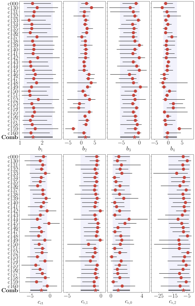
Figure 1: The median and 68th percentile of the best-fit EFT parameter distributions for the TNHOD M+Q configuration, prior to applying the NF model. Each panel represents one of the eight EFT parameters across 32 individual simulation boxes, with the combined case (Comb) shown at the bottom. The red points represent the median values for each box, and the horizontal error bars indicate the 68th percentile range of the best-fit distributions. The shaded regions represent the 68th percentile for the combined case.

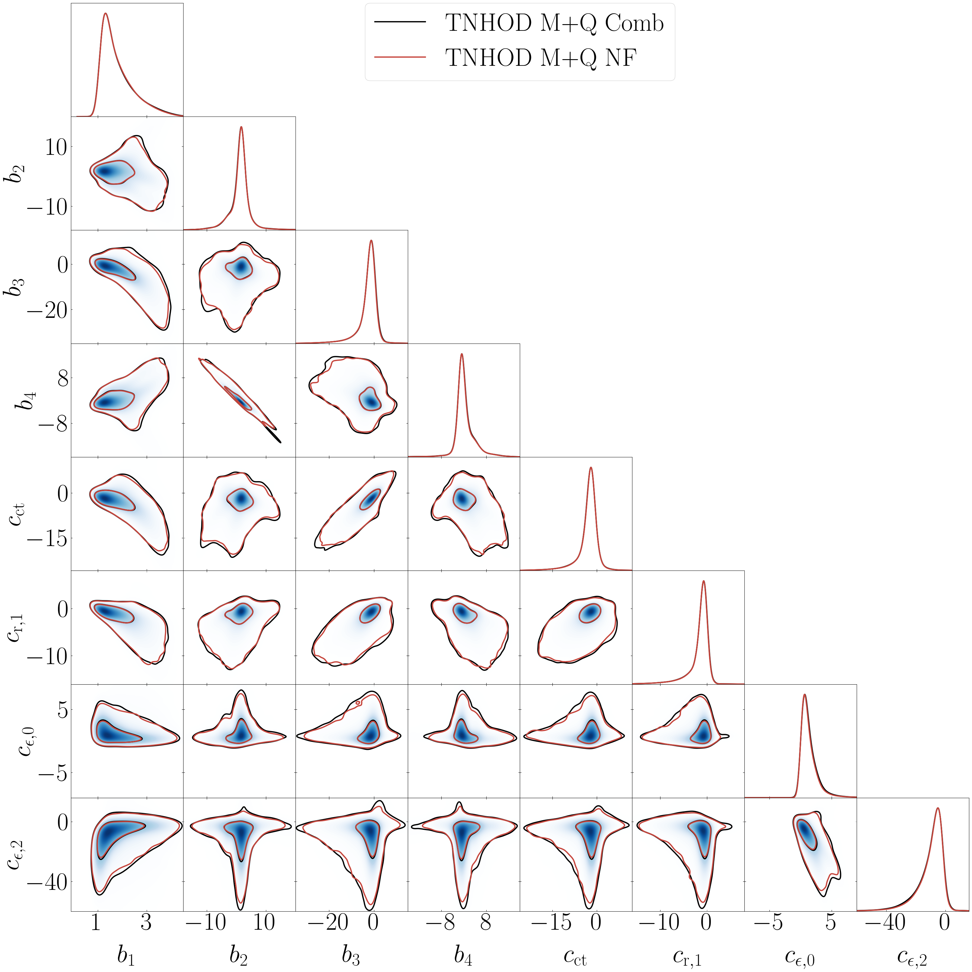
Figure 2: A comparison between the original combined best-fit EFT parameter distributions (black shaded contours) and the distributions learned by the NF model (red contours) for the TNHOD M+Q configuration. The diagonal panels show the 1D marginalized distributions, while the off-diagonal panels display the 1-$\sigma$ and 2-$\sigma$ contours.

Figure 1 displays the median and 68th percentile of the best-fit distribution under the TNHOD M+Q configuration, prior to applying the NF, for each individual simulation box as well as the combined case (Comb) across all 32 boxes. Each red point represents the median value of an EFT parameter, with the error bars denoting the 68th percentile range. The consistency between the individual boxes and the combined result is apparent for all EFT parameters explored, with most individual box distributions overlapping well with the combined case. This indicates that no strong cosmological dependency is observed in the EFT parameter distributions, ensuring the safety of using the HOD-informed prior when exploring the cosmological parameter space.

Figure 2 compares the true combined best-fit EFT parameter distributions (shaded black contours) to those learned by the NF model (red contours) for the TNHOD M+Q configuration. The 1D marginalized distributions and 1-$\sigma$ contours show excellent alignment between the true and NF-learned distributions. Only slight differences appear in the 2-$\sigma$ contour lines, demonstrating the NF model’s robustness in capturing the distribution, with minimal discrepancies at the outer edges.

4.2 Influence of HOD sample distribution and hexadecapole inclusion

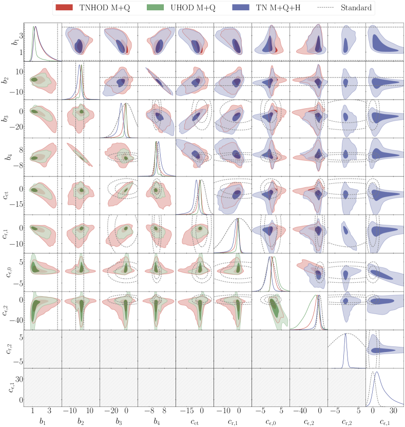
Figure 3: Contour plots illustrating the NF learned HOD-informed priors using three different configurations: TNHOD M+Q (red contours), UHOD M+Q (green contours), and TNHOD M+Q+H (blue contours). The unfilled gray contours (and boundary lines) represent the standard prior for EFTofLSS full-shape analysis as listed in Table 2 for comparison. Each contour indicates the 1-$\sigma$ and 2-$\sigma$ intervals of the distribution. The lower triangle compares the TNHOD M+Q and UHOD M+Q priors, highlighting the impact of removing the Gaussian component from the HOD sample distribution. The upper triangle compares the TNHOD M+Q and TNHOD M+Q+H priors, showing the effect of including the hexadecapole moment on the priors.

The NF-learned HOD-informed priors for the three configurations are displayed in Figure 3. In this figure, the red contours correspond to the TNHOD M+Q configuration, the green contours to the TNHOD M+Q+H configuration, and the slate blue contours to the UHOD M+Q configuration. For comparison, the standard EFTofLSS full-shape analysis prior, as listed in Table 2, is shown as a gray dashed contour.

Focusing on the lower triangle in this figure, we compare the impact of removing the Gaussian prior when sampling the HOD parameters. The most notable difference is observed in $b_{1}$, where the UHOD configuration shows a more concentrated $b_{1}$ distribution, indicated by a smaller 1-sigma contour area and 1D marginalized distribution. This occurs because $b_{1}$ is the most degenerate parameter with the HOD parameters. Specifically, in the UHOD configuration, we sample more combinations with large $\sigma$ and smaller $\log M_{\mathrm{cut}}$. These combinations tend to lead to smaller values of $b_{1}$.

From the HOD model perspective, larger $\sigma$ means that the transition from low to high probability of a halo hosting a galaxy is less steep, allowing a broader range of halo masses to contribute to the galaxy population. This more gradual transition results in a higher number of low-mass halos hosting galaxies, which generally have lower bias, thus reducing the overall galaxy bias. Similarly, a smaller $\log M_{\mathrm{cut}}$ lowers the threshold mass for halos to begin hosting galaxies, further increasing the contribution from low-mass halos. These low-mass halos, with lower bias, also contribute to reducing the overall value of $b_{1}$. Since $b_{1}$ represents the linear galaxy bias, its value is closely tied to the mass distribution and occupancy of galaxies within halos. The inclusion of more extreme HOD parameter combinations under the UHOD configuration therefore skews the $b_{1}$ distribution towards smaller values, reflecting these physical relationships.

Despite the differences in the distribution of $b_{1}$, the overall volume of the parameter space is smaller for the UHOD M+Q configuration compared to TNHOD M+Q, as indicated by the generally smaller 2-$\sigma$ contour sizes in most cases. As discussed earlier for $b_{1}$, the UHOD configuration allows for more galaxies to reside in low-mass host halos, leading to a different galaxy population compared to TNHOD. Consequently, the two configurations represent different types of galaxies, with TNHOD being more LRG-like, reflecting galaxies in more massive halos, while UHOD produces a more concentrated best-fit EFT distribution. However, aside from $b_{1}$, the peak values of the 1D distributions remain largely unchanged for most other parameters.

Next, we focus on the upper triangle in Figure 3, where we compare the impact of including the hexadecapole. For the M+Q cases, we set $c_{\mathrm{r,2}}$ to 0, as it is degenerate with $c_{\mathrm{r,1}}$. However, when we include the hexadecapole, $c_{\mathrm{r,2}}$ can be well constrained. Additionally, examining the 1D marginalized distributions, we observe slight shifts in several parameters with the inclusion of the hexadecapole. The higher-order bias terms $b_{2}$, $b_{3}$ and $b_{4}$ are affected as the hexadecapole provide more information about the anisotropic clustering of galaxies. The counterterm coefficient $c_{\mathrm{ct}}$ which account for corrections to non-linear effects, is influenced by the hexadecapole’s ability to distinguish velocity dispersion effects from galaxy clustering anisotropies. $c_{\epsilon,0}$ tends to favor smaller values due to the inclusion of $c_{\epsilon,1}$ as free parameter. Nevertheless, the distribution remains largely consistent between the M+Q and M+Q+H cases.

When comparing all HOD-informed priors with the standard prior, it is clear that the HOD-informed priors, regardless of the configuration, provide provide a detailed picture of the degeneracy directions between the EFT parameters, which the standard prior fails to capture. Additionally, for most parameters, the 1-$\sigma$ contour areas are significantly smaller for the HOD-informed priors, indicating a noticeable reduction in the effective EFT parameter space. This reduction shows that the HOD-informed priors help guide the exploration of a more physically meaningful parameter space, mitigating prior effects and ultimately leading to more accurate cosmological parameter posteriors.

5 Comparative analysis of priors

Model	$\Lambda$CDM			$w$CDM			$w_{0}w_{a}$CDM
Prior	Standard	TNHOD	UHOD	Standard	TNHOD	UHOD	Standard	TNHOD	UHOD
$\Omega_{c}h^{2}$	1.65(2.46)	0.57(1.36)	0.46	1.90(2.64)	1.03(1.44)	0.96	2.00(2.60)	1.00(1.39)	1.04
$H_{0}$	1.55(1.74)	0.87(1.08)	0.82	2.26(1.36)	1.57(0.88)	1.56	1.84(0.93)	1.76(1.04)	1.38
$\ln 10^{10}A_{s}$	1.46(1.61)	0.37(0.74)	0.22	2.55(1.95)	1.55(0.81)	1.42	2.89(1.61)	2.05(0.90)	1.72
$n_{s}$	1.88(2.12)	0.50(1.29)	0.32	1.97(2.31)	1.13(1.35)	0.96	2.09(2.31)	1.17(1.41)	1.06
$w$	-   (   -   )	-   (   -   )	-	1.97(0.80)	1.42(0.44)	1.40	0.72(0.21)	1.01(0.56)	0.64
$w_{a}$	-   (   -   )	-   (   -   )	-	-   (   -   )	-   (   -   )	-	0.59(0.13)	0.12(0.25)	0.17

Table 3: $\sigma$-distance values for all tested combinations of cosmological models and priors. This table compares results across the $\Lambda$CDM, $w$CDM and $w_{0}w_{a}$CDM cosmological models, using both the standard prior and HOD-informed priors (TNHOD and UHOD). The numbers outside of the brackets represent results from the M+Q case, while the numbers inside the brackets correspond to the M+Q+H case. For the UHOD prior, only the M+Q case is shown.

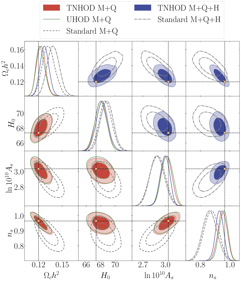
Figure 4: Marginalised posterior constraints obtained using different priors for $\Lambda\mathrm{CDM}$ model. The lower triangle shows the results using the monopole and quadrupole moments (M+Q), while the upper triangle includes the hexadecapole moment (M+Q+H). Red and green contours represent posteriors obtained with TNHOD and UHOD priors, respectively, for the M+Q case, while blue contours show TNHOD posteriors for the M+Q+H case. Dashed and dot-dash gray lines correspond to the standard prior results for M+Q and M+Q+H, respectively. Moccasin cross markers indicate the true values. All contours show 68$\%$ and 95$\%$ credible intervals.

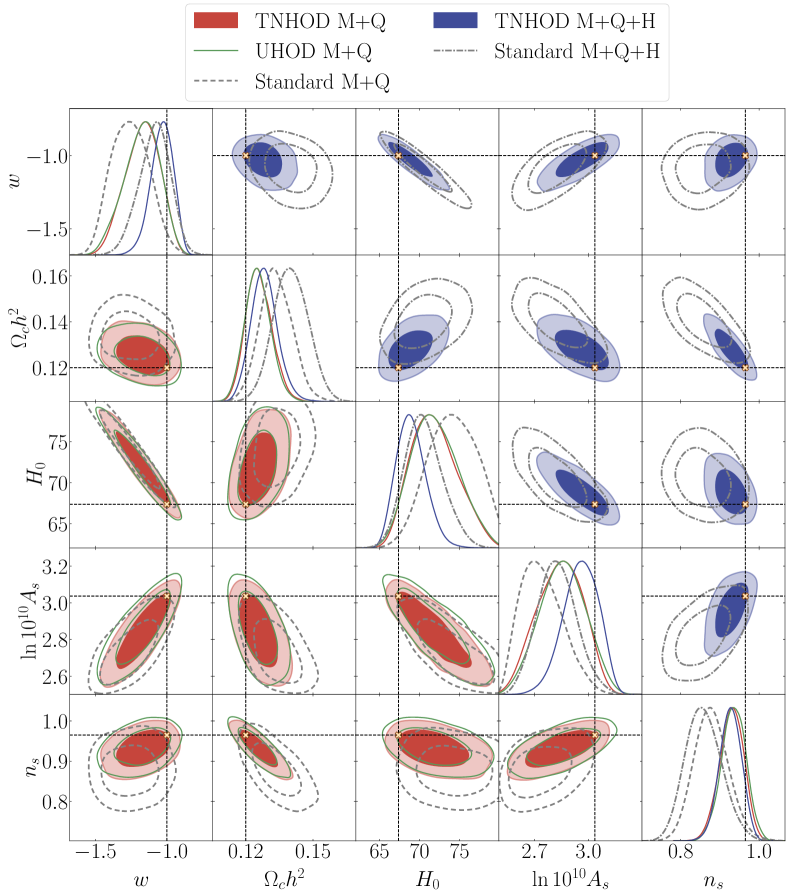
Figure 5: Similar plot as Figure 4 for $w\mathrm{CDM}$

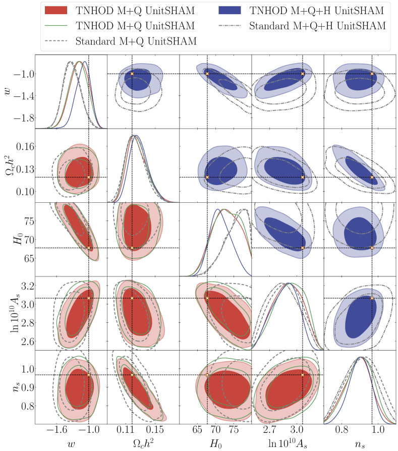
Figure 6: Similar plot as Figure 4 for $w\mathrm{CDM}$ using a SHAM-Unit mock

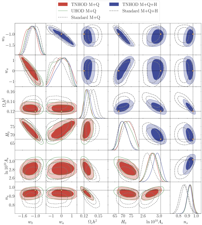
Figure 7: Similar plot as Figure 4 for $w_{0}w_{a}\mathrm{CDM}$

In this section, we perform a full-shape power spectrum analysis using the EFTofLSS redshift-space power spectrum model described in Section 2.2 to evaluate the improvement of the HOD-informed prior compared to the standard prior in reducing prior effects. Both cosmological parameters and EFT parameters are allowed to vary, with a Big Bang Nucleosynthesis (BBN) prior [98] imposed on the physical baryon density $\Omega_{b}h^{2}$. The cosmological parameters sampled include: $\Omega_{b}h^{2}$, $\Omega_{c}h^{2}$, respectively physical baryon and cold dark matter densities, $H_{0}$, the Hubble constant, $\ln 10^{10}A_{s}$, the amplitude of primordial scalar fluctuations, and $n_{s}$, the scalar spectral index.

To conduct this analysis, we prepared an DESI LRG-like HOD galaxy catalog using the
AbacusSummit_base_c000_ph000 box at redshift $z=0.8$. The HOD parameters used are based on those described in table 3 of [57] for LRG with $0.6<z<0.8$, with the galaxy density tuned to $5\times 10^{-4}\,{\rm Mpc}^{-3}$. We computed the power spectrum multipoles for this catalog, adopting 18 linear bins with a scale cut of $0.02<k<0.2\,h^{-1}\rm{Mpc}$ for the monopole, quadrupole, and hexadecapole moments. For the covariance matrix, we utilized the Gaussian Covariance from CovaPT, with linear bias, volume, and number density matching the catalog.

We proceed to fit with three different cosmological models: $\Lambda\mathrm{CDM}$, $w\mathrm{CDM}$, $w_{0}w_{a}\mathrm{CDM}$. For each model, we examine two cases: one using only the monopole and quadrupole moments (M+Q) and the other including the hexadecapole moment (M+Q+H). In the analyses without the hexadecapole, $c_{\mathrm{r,2}}$ and $c_{\mathrm{\epsilon,1}}$ are set to zero. The M+Q cases use the HOD-informed prior trained with M+Q data (red or green contours on Figure 3), while the M+Q+H cases use the HOD-informed prior trained with M+Q+H data (slate blue contours on Figure 3). We use the pocoMC as sampler [99, 100] and GetDist [101] to generate the contour plots. In this section we use PyBird to compute the theoretical model rather than effort.jl, to show that the emulator did not introduce any sizable error that could lead to biased results when using the HOD calibrated prior. We set the fiducial cosmology to match that of the simulation used to generate the mock. The Alcock-Paczynski effect is then applied by PyBird as described in Section 2.3.

To quantitatively describe the discrepancy between the resulting posteriors using different priors and the true cosmology, we use the $\sigma$-distance metric. For a certain parameter $X$, $\sigma$-$\mathrm{distance}=\left|X_{\mathrm{mean}}-X_{\mathrm{true}}\right|/\sigma$, where $X_{\mathrm{mean}}$ is the marginalised mean, $X_{\mathrm{true}}$ is the true value from the simulation, and $\sigma$ is the 1-$\sigma$ error. While it is not necessary that the truth lies within a Bayesian credible interval a certain fraction of the time - it is a frequentist test - it can be indicative of a bias within the Bayesian analysis caused by the prior. Table 3 shows the $\sigma$-distance values for all combinations of cosmological models and priors that have been tested. It is evident that the standard prior suffers significantly from prior effects, leading to a higher $\sigma$-distance and less accurate recovery of the true cosmology. In contrast, the HOD-informed priors (both TNHOD and UHOD) help mitigate these prior effects, consistently providing a more precise recovery of the true cosmological parameters across all models. We will discuss different cases in detail, along with the corresponding contour plots, in the following paragraphs.

Figure 4 presents contour plots comparing the performance of HOD-informed priors against standard priors in a full-shape analysis for the $\Lambda\mathrm{CDM}$ cosmological model. The plot is divided into two sections: the lower triangle shows results from the analysis using monopole and quadrupole moments (M+Q), while the upper triangle includes the hexadecapole moment (M+Q+H). The red contours represent the TNHOD prior for the M+Q case, the green contours represent the UHOD prior for the M+Q case, and the blue contours correspond to the TNHOD prior for the M+Q+H case. The dashed and dot-dash gray contours represent the standard prior for the M+Q and M+Q+H cases, respectively. Cross markers indicate the true values of the cosmological parameters. Note that $\Omega_{b}h^{2}$ is dominated by the BBN prior, so it is omitted from the contour plots.

The results made using the standard prior are significantly biased with the true cosmological parameters far from the credible regions. This is evident when comparing the HOD-informed prior contours (red, green, and blue) with the standard prior contours (gray dashed, gray dot-dashed) of Figure 4. On the other hand, all HOD-informed priors provide credible regions more consistent with the underlying cosmology, particularly for parameters such as $\Omega_{c}h^{2}$, $\ln 10^{10}A_{s}$ and $n_{s}$ compared to the standard prior. For example, focusing on the TNHOD M+Q (red) contours, the $\sigma$-distance for $\Omega_{c}h^{2}$ improves from 1.65 with the standard prior to 0.57. Similarly, for $\ln 10^{10}A_{s}$, the value improves from 1.46 to 0.37, and for $n_{s}$ , it drops from 1.88 to 0.50. Also for $H_{0}$, there is a notable improvement, with the $\sigma$-distance reduced from 1.55 to 0.87. These comparisons clearly demonstrate the ability of the HOD-informed prior to mitigate the prior effect. Note that though power spectrum alone has limited constraining power on $n_{s}$, it is still correlated with other parameters and EFT parameters. The HOD-informed prior, by reducing the degeneracies among those parameters, allows $n_{s}$ to be better recovered. The HOD-informed prior leads to tighter constraints by $28\%$, $9\%$, $29\%$, and $37\%$ for $\Omega_{c}h^{2}$, $H_{0}$, $\ln 10^{10}A_{s}$, and $n_{s}$, respectively, compared to the standard prior. Thus we see that the $\sigma$-distance improvements were not driven by having larger credible intervals, but instead by mitigating prior effects. This improvement in constraints is not driven by physical knowledge of the particular halos being modelled, as we have used a wide range of HOD parameters.

Another interesting point is that the posteriors using TNHOD and UHOD are nearly identical, indicating that the cosmological analysis, at least for the $\Lambda$CDM model, is not significantly influenced by the distribution of HOD sample used to generate the HOD-informed prior. Although the UHOD prior exhibits a more concentrated distribution, as shown in Figure 3, it does not lead to tighter constraints compared to the TNHOD prior.

Figure 5 present the contour plots for the $w\mathrm{CDM}$ model. In this case, the fit using the standard prior suffers from more severe prior effects due to the expanded parameter space. The $\sigma$-distance values for most parameters are around or exceed 2 in the M+Q case. Although the inclusion of the hexadecapole in the M+Q+H case provides some improvement, there are still significant deviations, with $\Omega_{c}h^{2}$ and $n_{s}$ showing over 2-$\sigma$ differences from the true values. In contrast, the HOD-informed prior (red and blue contours) consistently recovers the true values across all parameters. Taking the TNHOD M+Q case as an example, the $\sigma$-distance for $\Omega_{c}h^{2}$ decreases from 1.90 with the standard prior to 1.03, for $H_{0}$ from 2.26 to 1.57, for $\ln 10^{10}A_{s}$ from 2.55 to 1.55, for $n_{s}$ from 1.97 to 1.13. and for the parameter $w$, from 1.97 to 1.42. The green (UHOD M+Q) and red (TNHOD M+Q) contours match each other perfectly, constraining power using HOD-informed prior remaining similar as using standard prior, and the arguments made for the $\Lambda$CDM case still hold for the $w$CDM model.

Figure 6 presents contour plots for the $w\mathrm{CDM}$ cosmological model, similar to Figure 5, but with the analysis performed on a galaxy catalog generated using the Sub-Halo Abundance Matching (SHAM) approach [102, 103, 104, 105, 106, 107], also using a different simulation, UNIT [108]. This SHAM-based mock catalog is an DESI LRG-like mock from [109], at redshift $z=0.8188$ with a box size of 1000$h^{-1}\mathrm{Mpc}$ per side. Even though the simulation is different, the results are consistent with those observed in Figure 5. We also fit this mock with $\Lambda\mathrm{CDM}$ and $w_{0}w_{a}\mathrm{CDM}$ models, which both give similar results as using the Abacus mock. For brevity, we only show the contourplot for the $w\mathrm{CDM}$ model. The fact that the HOD-informed prior, when applied to galaxy catalogs generated using different galaxy-halo connection approaches, gives consistent results, makes us more confident about applying it to real observational data.

The results from fitting the $w_{0}w_{a}$CDM model are shown in Figure 7. Fits using the standard prior again lead to 1D credible intervals shifted from the truth, particularly for $\Omega_{c}h^{2}$, $\ln 10^{10}A_{s}$ and $n_{s}$. However, the inclusion of the hexadecapole seems to help in matching the credible intervals to the true values for $H_{0}$ and $\ln 10^{10}A_{s}$. Meanwhile, the HOD-informed priors continue to perform well, accurately matching intervals and the true cosmological parameters across the all cases. Interestingly, the UHOD prior (green contours) performs slightly better than the TNHOD prior (red contours) in this case, as indicated by the small shift in the 1 and 2 $\sigma$ contours. This is likely due to the use of a more flexible cosmological model and the fact that the data alone do not have enough constraining power. As a result, the more concentrated UHOD prior helped with a better recovery. However, the difference between the two is still small, and it is expected that when we combine more data from multiple redshifts, the dependency on the choice of the HOD sample distribution will again become minimal.

6 Conclusion

In this paper, we introduced an HOD-informed prior for the EFTofLSS framework to mitigate the prior effects commonly encountered in full-shape cosmological analyses of large-scale structure. We generated galaxy power spectra from a diverse set of HOD mock catalogs, covering a broad range of HOD parameter space and cosmological models. By fitting the EFTofLSS model to these power spectra, we extracted the best-fit EFT parameters and used their distribution to construct an HOD-informed prior. This approach provides a more physically motivated parameter space by mapping the EFT parameter space to a galaxy-halo connection framework.

We tested the robustness of our HOD-informed prior by analyzing its dependence on cosmological models, HOD sample distributions, and the inclusion of the hexadecapole moment. Our results showed that the distribution of EFT parameters does not exhibit specific dependencies on cosmology, making the prior largely cosmology-independent. Importantly, the HOD sample distribution does influence the HOD-informed prior, as it intrinsically represents different types of tracers.

We then conducted a full-shape analysis on a DESI LRG-like HOD catalog generated at redshift $z=0.8$. In general, the HOD-informed prior consistently outperformed the standard prior, mitigating prior effects across all three cosmological models we tested and under various configurations. For example, in the $\Lambda$CDM case, the $\sigma$-distance for $\Omega_{c}h^{2}$ improved from 1.65 with the standard prior to 0.57 with the HOD-informed prior. Similarly, in the $w$CDM model,it decreased from 1.90 to 1.03. In the more flexible $w_{0}w_{a}$CDM model, the HOD-informed prior brought the $\sigma$-distance down from 2.00 to 1.00. We achieved a good recovery of all cosmological parameters within credible regions, with detailed $\sigma$-distance values presented in Table 3. Those test on mock catalog highlight the robustness and effectiveness of the HOD-informed prior in recovering true cosmological parameters more precisely.

We further tested this using a SHAM-based mock from the UNIT simulation, and the consistent results demonstrate that our approach is simulation-independent. We also find that, while the HOD sample distribution does influence the shape of the prior itself, it has limited impact on cosmological fitting. Together, these findings confirm the robustness of the HOD-informed prior and its suitability for application to real observational data.

In future work, we aim to extend the current HOD model by incorporating assembly bias, allowing us to capture additional nonlinear information. By accounting for these missing nonlinear modes that the baseline model overlooks, we can further refine the HOD-informed prior, making it even more reliable for cosmological analyses. While this study has focused on LRG-like galaxies, we plan to expand the method to other tracers by adjusting the HOD models and sample distributions, allowing our approach to be applied across different galaxy populations and redshifts. This method could be extended to higher-order statistics, such as the bispectrum for additional information. The 1-loop EFT model for the bispectrum has more nuisance parameters compared to power spectrum, making it more sensitive to prior effects [37].

As current-generation surveys continue to produce more data, and with the arrival of next-generation surveys, the advantages of full-shape analysis will become increasingly evident. It is crucial to extract accurate cosmological information from the available data to address key questions, such as the Hubble constant tension and the $S_{8}$ tension, from a large-scale structure perspective. The HOD-informed prior presented in this paper will play an important role in the future, making full-shape analysis performance better, providing a robust tool for both current and upcoming surveys.

Appendix A Covariance matrix dependency

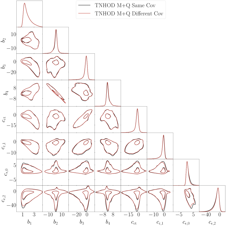
Figure 8: 68$\%$ and 95$\%$ contour plots compare the best-fit EFT parameter distributions for the TNHOD M+Q case using a single covariance matrix (black contours) and using a different covariance matrix for each power spectrum (red contours).

We test here whether the best-fit EFT parameter distribution depends on the covariance matrix used during the fitting process. By default, we employ a single analytical Gaussian covariance matrix, assuming a linear bias of 2 and a galaxy density of $5\times 10^{-4}\,{\rm Mpc}^{-3}$ for all fits. To investigate any dependence on the covariance matrix, we conduct a test for the TNHOD and M+Q case.

For each power spectrum we fit, we generate an analytical Gaussian covariance matrix based on the true linear bias and number density of the corresponding HOD mock catalog. This results in using a different covariance matrix for every power spectrum, amounting to 320,000 different covariance matrices in total.

Figure 8 shows that the best-fit EFT parameter distribution is nearly identical when using one single covariance matrix compared to using different covariance matrices for each fit. As our focus is on finding the best fits rather than exploring detailed EFT parameter distributions or degeneracies, it is safe to use the same covariance matrix for the best-fit finding. This also demonstrates that our EFT parameter best-fit distribution is effectively independent of the covariance matrix used.

Appendix B Check on the perturbativity of the prior

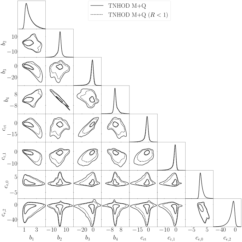
Figure 9: 68$\%$ and 95$\%$ contour plots compare the best-fit EFT parameter distributions for the TNHOD M+Q case with (dashed contours) and without (solid contours) a perturbative cut.

The EFTofLSS is based on the assumption that the model is being evaluated in the perturbative regime: if the contributions from the re-normalized loop-term happened to be bigger than the linear term, this would highlight a breakdown of the model and hence the non-reliability of the results.

In this appendix, we present the result of this check for the TNHOD M+Q case. For each best-fit combination, we compute the ratio

$$R=\frac{P_{\text{1-loop}}+P_{\text{ct}}}{P_{\text{lin}}},$$ (B.1)

where the subscript 1-loop, ct, and lin represent the 1-loop, counterterms, and linear contributions to the theoretical power spectrum monopole, respectively, at the highest $k$ considered in our fits. Only $3.1\%$ of the best fits show a ratio greater than 1, indicating that the vast majority of the best fits remain within the perturbative regime. We also would like to point out this be a consequence of the removal of best fits described in Sec. 3.3, when we removed points close to the boundary set on EFT parameters; given their large values, it was very likely they would have not passed the perturbativity test. Figure 9 shows the distributions of the best fits with (dashed) and without (solid) the perturbative cut. These two distributions exhibit nearly identical 1D marginalized distribution and 1-$\sigma$ contours, with only minor differences in their tails, as indicated by the difference in the 2-$\sigma$ contours. Given that the most of best-fit combinations comply with perturbative requirements and show minimal impact on the distribution, we conclude that using a prior with or without the perturbative cut does not significantly influence the analysis presented in this paper.

References

- [1] K.S. Dawson, D.J. Schlegel, C.P. Ahn, S.F. Anderson, E. Aubourg, S. Bailey et al., The Baryon Oscillation Spectroscopic Survey of SDSS-III, The Astronomical Journal 145 (2013) 10.
- [2] K.S. Dawson, J.-P. Kneib, W.J. Percival, S. Alam, F.D. Albareti, S.F. Anderson et al., The SDSS-IV Extended Baryon Oscillation Spectroscopic Survey: Overview and Early Data, The Astronomical Journal 151 (2016) 44.
- [3] M. Levi, C. Bebek, T. Beers, R. Blum, R. Cahn, D. Eisenstein et al., The DESI Experiment, a whitepaper for Snowmass 2013, arXiv e-prints (2013) arXiv:1308.0847.
- [4] DESI Collaboration, A. Aghamousa, J. Aguilar, S. Ahlen, S. Alam, L.E. Allen et al., The DESI Experiment Part I: Science,Targeting, and Survey Design, arXiv e-prints (2016) arXiv:1611.00036.
- [5] DESI Collaboration, A. Aghamousa, J. Aguilar, S. Ahlen, S. Alam, L.E. Allen et al., The DESI Experiment Part II: Instrument Design, arXiv e-prints (2016) arXiv:1611.00037.
- [6] D. Collaboration, B. Abareshi, J. Aguilar, S. Ahlen, S. Alam, D.M. Alexander et al., Overview of the Instrumentation for the Dark Energy Spectroscopic Instrument, The Astronomical Journal 164 (2022) 207.
- [7] Euclid Collaboration, Y. Mellier, Abdurro’uf, J.A. Acevedo Barroso, A. Achúcarro, J. Adamek et al., Euclid. I. Overview of the Euclid mission, arXiv e-prints (2024) arXiv:2405.13491.
- [8] Ž. Ivezić, S.M. Kahn, J.A. Tyson, B. Abel, E. Acosta, R. Allsman et al., LSST: From Science Drivers to Reference Design and Anticipated Data Products, The Astrophysical Journal 873 (2019) 111.
- [9] D. Spergel, N. Gehrels, C. Baltay, D. Bennett, J. Breckinridge, M. Donahue et al., Wide-Field InfrarRed Survey Telescope-Astrophysics Focused Telescope Assets WFIRST-AFTA 2015 Report, arXiv e-prints (2015) arXiv:1503.03757.
- [10] D. Baumann, A. Nicolis, L. Senatore and M. Zaldarriaga, Cosmological non-linearities as an effective fluid, Journal of Cosmology and Astroparticle Physics 2012 (2012) 051.
- [11] J.J.M. Carrasco, M.P. Hertzberg and L. Senatore, The effective field theory of cosmological large scale structures, Journal of High Energy Physics 2012 (2012) 82.
- [12] R.A. Porto, L. Senatore and M. Zaldarriaga, The Lagrangian-space Effective Field Theory of large scale structures, Journal of Cosmology and Astroparticle Physics 2014 (2014) 022.
- [13] A. Perko, L. Senatore, E. Jennings and R.H. Wechsler, Biased Tracers in Redshift Space in the EFT of Large-Scale Structure, arXiv e-prints (2016) arXiv:1610.09321.
- [14] T. Colas, G. d’Amico, L. Senatore, P. Zhang and F. Beutler, Efficient cosmological analysis of the SDSS/BOSS data from the Effective Field Theory of Large-Scale Structure, Journal of Cosmology and Astroparticle Physics 2020 (2020) 001.
- [15] G. d’Amico, J. Gleyzes, N. Kokron, K. Markovic, L. Senatore, P. Zhang et al., The cosmological analysis of the SDSS/BOSS data from the Effective Field Theory of Large-Scale Structure, Journal of Cosmology and Astroparticle Physics 2020 (2020) 005.
- [16] M.M. Ivanov, M. Simonović and M. Zaldarriaga, Cosmological parameters from the BOSS galaxy power spectrum, Journal of Cosmology and Astroparticle Physics 2020 (2020) 042.
- [17] G. D’Amico, L. Senatore and P. Zhang, Limits on wCDM from the EFTofLSS with the PyBird code, Journal of Cosmology and Astroparticle Physics 2021 (2021) 006.
- [18] F. Niedermann and M.S. Sloth, New early dark energy is compatible with current LSS data, Physical Review D 103 (2021) 103537.
- [19] S. Kumar, R.C. Nunes and P. Yadav, Updating non-standard neutrinos properties with Planck-CMB data and full-shape analysis of BOSS and eBOSS galaxies, Journal of Cosmology and Astroparticle Physics 2022 (2022) 060.
- [20] T. Simon, G.F. Abellán, P. Du, V. Poulin and Y. Tsai, Constraining decaying dark matter with BOSS data and the effective field theory of large-scale structures, Physical Review D 106 (2022) 023516.
- [21] R.C. Nunes, S. Vagnozzi, S. Kumar, E. Di Valentino and O. Mena, New tests of dark sector interactions from the full-shape galaxy power spectrum, Physical Review D 105 (2022) 123506.
- [22] O.H.E. Philcox and M.M. Ivanov, BOSS DR12 full-shape cosmology: CDM constraints from the large-scale galaxy power spectrum and bispectrum monopole, Physical Review D 105 (2022) 043517.
- [23] P. Zhang, G. D’Amico, L. Senatore, C. Zhao and Y. Cai, BOSS Correlation Function analysis from the Effective Field Theory of Large-Scale Structure, Journal of Cosmology and Astroparticle Physics 2022 (2022) 036.
- [24] S.-F. Chen, Z. Vlah and M. White, A new analysis of galaxy 2-point functions in the BOSS survey, including full-shape information and post-reconstruction BAO, Journal of Cosmology and Astroparticle Physics 2022 (2022) 008.
- [25] A. Laguë, J.R. Bond, R. Hložek, K.K. Rogers, D.J.E. Marsh and D. Grin, Constraining ultralight axions with galaxy surveys, Journal of Cosmology and Astroparticle Physics 2022 (2022) 049.
- [26] T. Simon, P. Zhang, V. Poulin and T.L. Smith, Consistency of effective field theory analyses of the BOSS power spectrum, Physical Review D 107 (2023) 123530.
- [27] P. Carrilho, C. Moretti and A. Pourtsidou, Cosmology with the EFTofLSS and BOSS: dark energy constraints and a note on priors, Journal of Cosmology and Astroparticle Physics 2023 (2023) 028.
- [28] N. Schöneberg, G.F. Abellán, T. Simon, A. Bartlett, Y. Patel and T.L. Smith, Comparative analysis of interacting stepped dark radiation, Physical Review D 108 (2023) 123513.
- [29] T.L. Smith, V. Poulin and T. Simon, Assessing the robustness of sound horizon-free determinations of the Hubble constant, Physical Review D 108 (2023) 103525.
- [30] I.J. Allali, F. Rompineve and M.P. Hertzberg, Dark sectors with mass thresholds face cosmological datasets, Physical Review D 108 (2023) 023527.
- [31] T. Simon, P. Zhang and V. Poulin, Cosmological inference from the EFTofLSS: the eBOSS QSO full-shape analysis, Journal of Cosmology and Astroparticle Physics 2023 (2023) 041.
- [32] T. Simon, P. Zhang, V. Poulin and T.L. Smith, Updated constraints from the effective field theory analysis of the BOSS power spectrum on early dark energy, Physical Review D 107 (2023) 063505.
- [33] G. D’Amico, Y. Donath, L. Senatore and P. Zhang, Limits on clustering and smooth quintessence from the EFTofLSS, Journal of Cosmology and Astroparticle Physics 2024 (2024) 032.
- [34] P. Collaboration, N. Aghanim, Y. Akrami, M. Ashdown, J. Aumont, C. Baccigalupi et al., Planck 2018 results. VI. Cosmological parameters, Astronomy and Astrophysics 641 (2020) A6.
- [35] A.G. Riess, S. Casertano, W. Yuan, L.M. Macri and D. Scolnic, Large Magellanic Cloud Cepheid Standards Provide a 1% Foundation for the Determination of the Hubble Constant and Stronger Evidence for Physics beyond CDM, The Astrophysical Journal 876 (2019) 85.
- [36] A. Gómez-Valent, Fast test to assess the impact of marginalization in Monte Carlo analyses and its application to cosmology, Physical Review D 106 (2022) 063506.
- [37] G. D’Amico, Y. Donath, M. Lewandowski, L. Senatore and P. Zhang, The BOSS bispectrum analysis at one loop from the Effective Field Theory of Large-Scale Structure, JCAP 05 (2024) 059 [2206.08327].
- [38] E.B. Holm, L. Herold, T. Simon, E.G.M. Ferreira, S. Hannestad, V. Poulin et al., Bayesian and frequentist investigation of prior effects in EFT of LSS analyses of full-shape BOSS and eBOSS data, Physical Review D 108 (2023) 123514.
- [39] Y.P. Jing, H.J. Mo and G. Börner, Spatial Correlation Function and Pairwise Velocity Dispersion of Galaxies: Cold Dark Matter Models versus the Las Campanas Survey, The Astrophysical Journal 494 (1998) 1.
- [40] J.A. Peacock and R.E. Smith, Halo occupation numbers and galaxy bias, Monthly Notices of the Royal Astronomical Society 318 (2000) 1144.
- [41] U. Seljak, Analytic model for galaxy and dark matter clustering, Monthly Notices of the Royal Astronomical Society 318 (2000) 203.
- [42] R. Scoccimarro, R.K. Sheth, L. Hui and B. Jain, How Many Galaxies Fit in a Halo? Constraints on Galaxy Formation Efficiency from Spatial Clustering, The Astrophysical Journal 546 (2001) 20.
- [43] A. Cooray and R. Sheth, Halo models of large scale structure, Physics Reports 372 (2002) 1.
- [44] A.A. Berlind and D.H. Weinberg, The Halo Occupation Distribution: Toward an Empirical Determination of the Relation between Galaxies and Mass, The Astrophysical Journal 575 (2002) 587.
- [45] Z. Zheng, A.A. Berlind, D.H. Weinberg, A.J. Benson, C.M. Baugh, S. Cole et al., Theoretical Models of the Halo Occupation Distribution: Separating Central and Satellite Galaxies, The Astrophysical Journal 633 (2005) 791.
- [46] Z. Zheng, A.L. Coil and I. Zehavi, Galaxy Evolution from Halo Occupation Distribution Modeling of DEEP2 and SDSS Galaxy Clustering, The Astrophysical Journal 667 (2007) 760.
- [47] Z. Zheng, I. Zehavi, D.J. Eisenstein, D.H. Weinberg and Y.P. Jing, Halo Occupation Distribution Modeling of Clustering of Luminous Red Galaxies, The Astrophysical Journal 707 (2009) 554.
- [48] M. White, M. Blanton, A. Bolton, D. Schlegel, J. Tinker, A. Berlind et al., The Clustering of Massive Galaxies at z ~ 0.5 from the First Semester of BOSS Data, The Astrophysical Journal 728 (2011) 126.
- [49] J. Richardson, Z. Zheng, S. Chatterjee, D. Nagai and Y. Shen, The Halo Occupation Distribution of SDSS Quasars, The Astrophysical Journal 755 (2012) 30.
- [50] Z. Zhai, J.L. Tinker, C. Hahn, H.-J. Seo, M.R. Blanton, R. Tojeiro et al., The Clustering of Luminous Red Galaxies at z 0.7 from EBOSS and BOSS Data, The Astrophysical Journal 848 (2017) 76.
- [51] S. Alam, J.A. Peacock, K. Kraljic, A.J. Ross and J. Comparat, Multitracer extension of the halo model: probing quenching and conformity in eBOSS, Monthly Notices of the Royal Astronomical Society 497 (2020) 581.
- [52] S. Avila, V. Gonzalez-Perez, F.G. Mohammad, A. de Mattia, C. Zhao, A. Raichoor et al., The Completed SDSS-IV extended Baryon Oscillation Spectroscopic Survey: exploring the halo occupation distribution model for emission line galaxies, Monthly Notices of the Royal Astronomical Society 499 (2020) 5486.
- [53] A. Smith, E. Burtin, J. Hou, R. Neveux, A.J. Ross, S. Alam et al., The completed SDSS-IV extended Baryon Oscillation Spectroscopic Survey: N-body mock challenge for the quasar sample, Monthly Notices of the Royal Astronomical Society 499 (2020) 269.
- [54] R. Zhou, J.A. Newman, Y.-Y. Mao, A. Meisner, J. Moustakas, A.D. Myers et al., The clustering of DESI-like luminous red galaxies using photometric redshifts, Monthly Notices of the Royal Astronomical Society 501 (2021) 3309.
- [55] G. Rossi, P.D. Choi, J. Moon, J.E. Bautista, H. Gil-Marín, R. Paviot et al., The completed SDSS-IV extended Baryon Oscillation Spectroscopic Survey: N-body mock challenge for galaxy clustering measurements, Monthly Notices of the Royal Astronomical Society 505 (2021) 377.
- [56] H. Zhang, L. Samushia, D. Brooks, A. de la Macorra, P. Doel, E. Gaztañaga et al., Constraining galaxy-halo connection with high-order statistics, Monthly Notices of the Royal Astronomical Society 515 (2022) 6133.
- [57] S. Yuan, H. Zhang, A.J. Ross, J. Donald-McCann, B. Hadzhiyska, R.H. Wechsler et al., The DESI one-per cent survey: exploring the halo occupation distribution of luminous red galaxies and quasi-stellar objects with ABACUSSUMMIT, Monthly Notices of the Royal Astronomical Society 530 (2024) 947.
- [58] A. Rocher, V. Ruhlmann-Kleider, E. Burtin, S. Yuan, A. de Mattia, A.J. Ross et al., The DESI One-Percent survey: exploring the Halo Occupation Distribution of Emission Line Galaxies with ABACUSSUMMIT simulations, Journal of Cosmology and Astroparticle Physics 2023 (2023) 016.
- [59] M.M. Ivanov, C. Cuesta-Lazaro, S. Mishra-Sharma, A. Obuljen and M.W. Toomey, Full-shape analysis with simulation-based priors: constraints on single field inflation from BOSS, arXiv e-prints (2024) arXiv:2402.13310.
- [60] M.M. Ivanov, A. Obuljen, C. Cuesta-Lazaro and M.W. Toomey, Full-shape analysis with simulation-based priors: cosmological parameters and the structure growth anomaly, arXiv e-prints (2024) arXiv:2409.10609.
- [61] R.H. Wechsler, J.S. Bullock, J.R. Primack, A.V. Kravtsov and A. Dekel, Concentrations of Dark Halos from Their Assembly Histories, The Astrophysical Journal 568 (2002) 52.
- [62] L. Gao, V. Springel and S.D.M. White, The age dependence of halo clustering, Monthly Notices of the Royal Astronomical Society 363 (2005) L66.
- [63] D.J. Croton, L. Gao and S.D.M. White, Halo assembly bias and its effects on galaxy clustering, Monthly Notices of the Royal Astronomical Society 374 (2007) 1303.
- [64] L. Gao and S.D.M. White, Assembly bias in the clustering of dark matter haloes, Monthly Notices of the Royal Astronomical Society 377 (2007) L5.
- [65] Y.-T. Lin, R. Mandelbaum, Y.-H. Huang, H.-J. Huang, N. Dalal, B. Diemer et al., On Detecting Halo Assembly Bias with Galaxy Populations, The Astrophysical Journal 819 (2016) 119.
- [66] A. Pujol, K. Hoffmann, N. Jiménez and E. Gaztañaga, What determines large scale galaxy clustering: halo mass or local density?, Astronomy and Astrophysics 598 (2017) A103.
- [67] M.C. Artale, I. Zehavi, S. Contreras and P. Norberg, The impact of assembly bias on the halo occupation in hydrodynamical simulations, Monthly Notices of the Royal Astronomical Society 480 (2018) 3978.
- [68] I. Zehavi, S. Contreras, N. Padilla, N.J. Smith, C.M. Baugh and P. Norberg, The Impact of Assembly Bias on the Galaxy Content of Dark Matter Halos, The Astrophysical Journal 853 (2018) 84.
- [69] B. Hadzhiyska, S. Bose, D. Eisenstein, L. Hernquist and D.N. Spergel, Limitations to the ‘basic’ HOD model and beyond, Monthly Notices of the Royal Astronomical Society 493 (2020) 5506.
- [70] X. Xu, I. Zehavi and S. Contreras, Dissecting and modelling galaxy assembly bias, Monthly Notices of the Royal Astronomical Society 502 (2021) 3242.
- [71] X. Xu, S. Kumar, I. Zehavi and S. Contreras, Predicting halo occupation and galaxy assembly bias with machine learning, Monthly Notices of the Royal Astronomical Society 507 (2021) 4879.
- [72] A.M. Delgado, D. Wadekar, B. Hadzhiyska, S. Bose, L. Hernquist and S. Ho, Modelling the galaxy-halo connection with machine learning, Monthly Notices of the Royal Astronomical Society 515 (2022) 2733.
- [73] A.N. Salcedo, Y. Zu, Y. Zhang, H. Wang, X. Yang, Y. Wu et al., Elucidating galaxy assembly bias in SDSS, Science China Physics, Mechanics, and Astronomy 65 (2022) 109811.
- [74] S. Yuan, B. Hadzhiyska, S. Bose and D.J. Eisenstein, Illustrating galaxy-halo connection in the DESI era with ILLUSTRISTNG, Monthly Notices of the Royal Astronomical Society 512 (2022) 5793.
- [75] K. Wang, Y.-Y. Mao, A.R. Zentner, H. Guo, J.U. Lange, F.C. van den Bosch et al., Evidence of galaxy assembly bias in SDSS DR7 galaxy samples from count statistics, Monthly Notices of the Royal Astronomical Society 516 (2022) 4003.
- [76] S. Yuan, R.H. Wechsler, Y. Wang, M.A.C. de los Reyes, J. Myles, A. Rocher et al., Unraveling emission line galaxy conformity at z-0.5ex1 with DESI early data, arXiv e-prints (2023) arXiv:2310.09329.
- [77] G. D’Amico, L. Senatore, P. Zhang and T. Nishimichi, Taming redshift-space distortion effects in the EFTofLSS and its application to data, Journal of Cosmology and Astroparticle Physics 2024 (2024) 037.
- [78] M.M. Ivanov, O.H.E. Philcox, M. Simonović, M. Zaldarriaga, T. Nischimichi and M. Takada, Cosmological constraints without nonlinear redshift-space distortions, Physical Review D 105 (2022) 043531.
- [79] L. Senatore and M. Zaldarriaga, Redshift Space Distortions in the Effective Field Theory of Large Scale Structures, arXiv e-prints (2014) arXiv:1409.1225.
- [80] L. Senatore and M. Zaldarriaga, The IR-resummed Effective Field Theory of Large Scale Structures, Journal of Cosmology and Astroparticle Physics 2015 (2015) 13.
- [81] M. Lewandowski and L. Senatore, An analytic implementation of the IR-resummation for the BAO peak, Journal of Cosmology and Astroparticle Physics 2020 (2020) 018.
- [82] L.H. Garrison, D.J. Eisenstein, D. Ferrer, M.V. Metchnik and P.A. Pinto, Improving initial conditions for cosmological N-body simulations, Monthly Notices of the Royal Astronomical Society 461 (2016) 4125.
- [83] L.H. Garrison, D.J. Eisenstein, D. Ferrer, J.L. Tinker, P.A. Pinto and D.H. Weinberg, The Abacus Cosmos: A Suite of Cosmological N-body Simulations, The Astrophysical Journal Supplement Series 236 (2018) 43.
- [84] L.H. Garrison, D.J. Eisenstein and P.A. Pinto, A high-fidelity realization of the Euclid code comparison N-body simulation with ABACUS, Monthly Notices of the Royal Astronomical Society 485 (2019) 3370.
- [85] L.H. Garrison, D.J. Eisenstein, D. Ferrer, N.A. Maksimova and P.A. Pinto, The ABACUS cosmological N-body code, Monthly Notices of the Royal Astronomical Society 508 (2021) 575.
- [86] S. Bose, D.J. Eisenstein, B. Hadzhiyska, L.H. Garrison and S. Yuan, Constructing high-fidelity halo merger trees in ABACUSSUMMIT, Monthly Notices of the Royal Astronomical Society 512 (2022) 837.
- [87] B. Hadzhiyska, D. Eisenstein, S. Bose, L.H. Garrison and N. Maksimova, COMPASO: A new halo finder for competitive assignment to spherical overdensities, Monthly Notices of the Royal Astronomical Society 509 (2022) 501.
- [88] S. Yuan, L.H. Garrison, B. Hadzhiyska, S. Bose and D.J. Eisenstein, ABACUSHOD: a highly efficient extended multitracer HOD framework and its application to BOSS and eBOSS data, Monthly Notices of the Royal Astronomical Society 510 (2022) 3301.
- [89] M. Bonici and G. D’Amico, effort.jl, arXiv e-prints (in prep) .
- [90] M. Bonici, F. Bianchini and J. Ruiz-Zapatero, Capse.jl: efficient and auto-differentiable CMB power spectra emulation, 2307.14339.
- [91] H. Ge, K. Xu and Z. Ghahramani, Turing: A Language for Flexible Probabilistic Inference, in Proceedings of the Twenty-First International Conference on Artificial Intelligence and Statistics, A. Storkey and F. Perez-Cruz, eds., vol. 84 of Proceedings of Machine Learning Research, pp. 1682–1690, PMLR, 9, 2018, https://proceedings.mlr.press/v84/ge18b.html.
- [92] D.C. Liu and J. Nocedal, On the limited memory BFGS method for large scale optimization, Mathematical Programming 45 (1989) 503.
- [93] D. Wadekar and R. Scoccimarro, Galaxy power spectrum multipoles covariance in perturbation theory, Physical Review D 102 (2020) 123517.
- [94] D. Jimenez Rezende and S. Mohamed, Variational Inference with Normalizing Flows, arXiv e-prints (2015) arXiv:1505.05770.
- [95] C. Durkan, A. Bekasov, I. Murray and G. Papamakarios, Neural Spline Flows, arXiv e-prints (2019) arXiv:1906.04032.
- [96] A. Paszke, S. Gross, F. Massa, A. Lerer, J. Bradbury, G. Chanan et al., PyTorch: An Imperative Style, High-Performance Deep Learning Library, arXiv e-prints (2019) arXiv:1912.01703.
- [97] D.P. Kingma and J. Ba, Adam: A Method for Stochastic Optimization, arXiv e-prints (2014) arXiv:1412.6980.
- [98] N. Schöneberg, The 2024 BBN baryon abundance update, Journal of Cosmology and Astroparticle Physics 2024 (2024) 006.
- [99] M. Karamanis, F. Beutler, J.A. Peacock, D. Nabergoj and U. Seljak, Accelerating astronomical and cosmological inference with preconditioned Monte Carlo, Monthly Notices of the Royal Astronomical Society 516 (2022) 1644.
- [100] M. Karamanis, D. Nabergoj, F. Beutler, J. Peacock and U. Seljak, pocoMC: A Python package for accelerated Bayesian inference in astronomy and cosmology, The Journal of Open Source Software 7 (2022) 4634.
- [101] A. Lewis, GetDist: a Python package for analysing Monte Carlo samples, arXiv e-prints (2019) arXiv:1910.13970.
- [102] A.V. Kravtsov, A.A. Berlind, R.H. Wechsler, A.A. Klypin, S. Gottlöber, B. Allgood et al., The Dark Side of the Halo Occupation Distribution, The Astrophysical Journal 609 (2004) 35.
- [103] A. Vale and J.P. Ostriker, Linking halo mass to galaxy luminosity, Monthly Notices of the Royal Astronomical Society 353 (2004) 189.
- [104] C. Conroy, R.H. Wechsler and A.V. Kravtsov, Modeling Luminosity-dependent Galaxy Clustering through Cosmic Time, The Astrophysical Journal 647 (2006) 201.
- [105] A. Vale and J.P. Ostriker, The non-parametric model for linking galaxy luminosity with halo/subhalo mass, Monthly Notices of the Royal Astronomical Society 371 (2006) 1173.
- [106] P.S. Behroozi, C. Conroy and R.H. Wechsler, A Comprehensive Analysis of Uncertainties Affecting the Stellar Mass-Halo Mass Relation for 0 < z < 4, The Astrophysical Journal 717 (2010) 379.
- [107] H. Guo, Z. Zheng, P.S. Behroozi, I. Zehavi, C.-H. Chuang, J. Comparat et al., Modelling galaxy clustering: halo occupation distribution versus subhalo matching, Monthly Notices of the Royal Astronomical Society 459 (2016) 3040.
- [108] C.-H. Chuang, G. Yepes, F.-S. Kitaura, M. Pellejero-Ibanez, S. Rodríguez-Torres, Y. Feng et al., UNIT project: Universe N-body simulations for the Investigation of Theoretical models from galaxy surveys, Monthly Notices of the Royal Astronomical Society 487 (2019) 48.
- [109] J. Yu, C. Zhao, V. Gonzalez-Perez, C.-H. Chuang, A. Brodzeller, A. de Mattia et al., The DESI One-Percent Survey: exploring a generalized SHAM for multiple tracers with the UNIT simulation, Monthly Notices of the Royal Astronomical Society 527 (2024) 6950.