Entanglement-enhanced quantum sensing via optimal global control

Abstract

We present a deterministic protocol for the preparation of arbitrary entangled states in the symmetric Dicke subspace of $N$ spins coupled to a common cavity mode. By combining a new geometric phase gate, an analytic solution of the noisy quantum channel dynamics and optimal control methods, the protocol prepares entangled states that are useful for quantum sensing, achieving a precision significantly better than the standard quantum limit in the presence of photon cavity loss, spontaneous emission and dephasing. This work opens the way to entanglement-enhanced sensing with cold trapped atoms in cavities and is also directly relevant for experiments with trapped ions.

Multi-particle entanglement is an essential resource for achieving quantum advantage in computing and sensing [1, 2], however it is fragile to errors. Quantum error correction (QEC) provides a general approach to protect entanglement from noise in quantum computers. However, a similar general approach does not exist for sensing because quantum sensors need to be simultaneously sensitive to the unknown field strength they are measuring but insensitive to noise. When the signal lies in the span of the noise operators, which is typically the case, then standard signal preserving QEC will not improve precision beyond the standard quantum limit (SQL) [3, 4] (although, adaptive, finite round QEC can circumvent this obstacle [5]). Thus, while entangled quantum states can in principle lead to Heisenberg limited precision, decoherence appears to limit the advantage. Indeed, experiments have so far relied on preparing simpler, spin squeezed states that are somewhat robust to noise, but that achieve measurement uncertainties scaling only moderately better than the SQL [6, 7, 8, 9, 10].

In this work, we present a deterministic protocol to prepare entangled states in the symmetric Dicke subspace of $N$ spins that are useful for sensing and optimally robust in the presence of a noisy environment. There are different approaches to this task, for example one can target states that maximize the quantum Fisher information in the presence of noise [11] but that doesn’t guarantee the states or the measured observable are efficiently constructed. We focus on spins coupled to a common cavity mode in the regime of strong coupling of cavity quantum electrodynamics, as can be realized, for example, with cold atoms trapped in optical cavities. Our noise-informed protocol combines a cavity driven geometric phase gate presented in the companion work [12], with an analytical approach to the solution of noisy channel quantum dynamics and optimal control methods to shape the laser pulses – i.e. the classical photon field driving the cavity mode and the global laser driving collective spin rotations. When applied to the measurement of the strength of a weak external field, the protocol prepares multi-particle entangled states leading to a scaling with $N$ of the measurement precision characterised by the variance of the estimated field strength that is significantly better than the SQL in the presence of relevant noise, such as photon cavity loss, spontaneous emission and dephasing already for moderately large strengths of light-matter interactions. Surprisingly, the protocol requires only a few global pulses of the cavity mode drive and global rotations, whose parameters we provide. We discuss the performance of different classes of entangled states that can be prepared using the protocol for field signal acquisition in the presence of spin dephasing. Using realistic estimates for parameters from current experiments, we find that neutral atoms are excellent candidates for entanglement-enhanced metrology. The approach can be extended to other platforms, e.g. trapped ions or Rydberg atoms.

We consider a setup consisting of $N$ three-level spin systems with computational qubit basis states $\ket{0}$ and $\ket{1}$ and an excited state $\ket{e}$. The levels $|1\rangle$ and $|e\rangle$ are coupled via a cavity mode with annihilation (creation) operators $\hat{a}$($\hat{a}^{\dagger})$ with coupling strength $g$ (Fig. 1(a)). The cavity mode is driven by a complex classical field of strength $\eta(t)$ which is detuned from the cavity and the $\ket{1}\leftrightarrow\ket{e}$ transition by $\delta$ and $\Delta$, respectively. The relevant Hamiltonian reads

$$\hat{H}=\delta\hat{a}^{\dagger}\hat{a}+\left(\Delta-i\frac{\gamma}{2}\right)\hat{n}_{e}+\left[\left(g\hat{S}^{-}+i\eta(t)\right)\hat{a}^{\dagger}+\mathrm{h.c.}\right]$$

with $\hat{n}_{e}=\sum_{j}|e_{j}\rangle\langle e_{j}|$, $\hat{S}^{+}=\sum_{j}|e_{j}\rangle\langle 1_{j}|$, $\hat{S}^{-}=(\hat{S}^{+})^{\dagger}$, and $\gamma$ the spontaneous emission rate from $\ket{e}$ state.

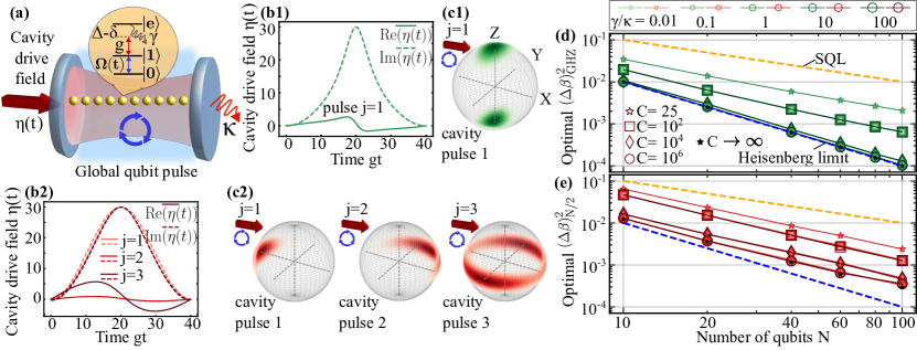
Figure 1: (a) A register of spins with states $\{|0\rangle,|1\rangle,|e\rangle\}$ is coupled to a cavity mode with coupling strength $g$ addressing the $\ket{1}\leftrightarrow\ket{e}$ transition, with detuning $\Delta-\delta$. The cavity mode is externally driven by a laser with amplitude $|\eta(t)|$, and a global laser pulse is applied on the $\ket{0}\leftrightarrow\ket{1}$ spin transition. Panels (b1,b2): Cavity drive pulses of the optimal state preparation protocol for $N=40$, $C=10^{4}$ and $\gamma/\kappa=0.01$, for GHZ-like and Dicke-like states, respectively. Throughout, we make a choice of the cavity drive pulse $\zeta(t)$ in the effective frame with $\mathrm{Re}(\zeta(t))=-2\delta\sqrt{\frac{2\phi}{3\delta T}}\sin^{2}(\frac{\pi t}{T})$ and $\mathrm{Im(\zeta(t))}=-\partial_{t}\mathrm{Re}(\zeta(t))/\delta$ (see [13] and [12]). The obtained minimal measurement precision variances here are $N(\Delta\beta)^{2}_{\mathrm{GHZ}}=0.03$ and $N(\Delta\beta)^{2}_{N/2}=0.08$. The parameters used in optimal state preparation protocol are listed in the Supplemental Material. (c1, c2): State trajectories in Husimi-Q representation of the spin states in the symmetric Dicke subspace after the application of each protocol step $j\,\forall j=1,\dots,P$. (d) Optimal $(\Delta\beta)^{2}_{\mathrm{GHZ}}$ for $P=1$ and (e) $(\Delta\beta)^{2}_{N/2}$ for $P=3$ obtained as a function of number of qubits $N$, plotted for spin-cavity cooperativities $C=25$ with $\gamma/\kappa=1$, and $C=10^{2},10^{4},10^{6}$ with different ratios $\gamma/\kappa=0.01,0.1,1,10,100$, obtained for the case of $gT\rightarrow\infty$. The optimal states prepared in the presence of finite $C$ successfully surpass the SQL for values as small as $C=25$.

In the companion work [12], we show that in the limit of strong cavity driving $\eta/g\rightarrow\infty$ and large detuning $\Delta/g\rightarrow\infty$, and $\delta=\mathcal{O}(g)$, the system dynamics can be reduced to the effective Hamiltonian

$$\hat{H}_{\mathrm{\mathrm{eff}}}=\delta\hat{a}^{\dagger}\hat{a}+\left(-i\frac{\gamma_{1}}{2}+\zeta\hat{a}^{\dagger}+\zeta^{*}\hat{a}\right)\hat{n}_{1},$$ (1)

with $\hat{n}_{1}=\sum_{j}\ket{1_{j}}\bra{1_{j}}$, $\gamma_{1}=\gamma(1-\sqrt{1-4|\zeta|^{2}/g^{2}})/2$, and $\zeta=g^{2}\alpha/\sqrt{4g^{2}|\alpha|^{2}+\Delta^{2}}$ where $\dot{\alpha}=-\eta-(i\delta+\kappa/2)\alpha$ with $\alpha(t=0)=0$. Here we recall the basic elements of the derivation: Eq. (1) is obtained from $\hat{H}$ by first moving into a frame rotating with the cavity by applying a time-dependent displacement operator $\hat{D}(\alpha(t))=\exp(\alpha\hat{a}^{\dagger}-\alpha^{*}\hat{a})$, with the amplitude $\alpha(t)$. The $\eta,\kappa-$dependent choice of $\alpha$ ensures that in the rotated frame the cavity drive $\eta(t)$ effectively appears as a collective drive of the qubits as $-g(\alpha\hat{S}^{+}+\alpha^{*}\hat{S}^{-})$. Further rotating in a frame that diagonalizes the qubit subspace in the limit $\Delta/g\rightarrow\infty$ and assuming that $n_{e}=0$ at time $t=0$ leads to Eq. (1). Interestingly, Eq. (1) is equivalent up to single spin rotations to the Mølmer-Sørensen Hamiltonian [14], originally developed for trapped ions, and can be thus used to generate fast geometric phase gates – albeit now for spin systems coupled to a cavity [12].

In this work, we are interested in the open system dynamics determined by Eq. (1) containing the non-hermitian contribution of $\gamma$ and within a Lindblad master equation approach with $\dot{\rho}=-i\hat{H}_{\mathrm{eff}}\rho+i\rho\hat{H}_{\mathrm{eff}}^{\dagger}+\hat{L}\rho\hat{L}^{\dagger}-\{\hat{L}^{\dagger}\hat{L},\rho\}/2$, with $\rho$ the system density matrix and $\hat{L}=\sqrt{\kappa}\hat{a}$ the jump operator where $\kappa$ is the the cavity mode decay rate [15].

We define the quantum channel of the geometric phase gate (realised with a single cavity drive of duration $T$) acting on a basis state $|q_{n}\rangle\langle q_{m}|$ of the qubit density matrix, where $\hat{n}_{1}|q_{n}\rangle=n|q_{n}\rangle$, ($q\in\{0,1\}^{N}$) as

$$\mathcal{E}_{\mathrm{gpg}}(\ket{q_{n}}\bra{q_{m}})=e^{i\varphi_{nm}(T)}\ket{q_{n}}\bra{q_{m}}.$$ (2)

The channel $\mathcal{E}_{\mathrm{gpg}}$ is obtained after tracing out the cavity from the joint spin-cavity state, which results in phase accumulation as a function of $n,m$ (i.e., the number of qubits in the $|1\rangle$ state). We then combine the dynamics obtained from Eq. (2) with optimal control methods to steer the collective symmetric (Dicke) states of $N$ spin qubits into entangled states of metrological use that are robust to relevant noise sources, such as loss of photons from the cavity mode with rate $\kappa$, loss of population from the excited state $|e\rangle$ with rate $\gamma$ and dephasing in the qubit subspace with rate $\gamma_{\phi}$. This is achieved by (i) solving analytically the Lindblad master equation to obtain the geometric phases $\varphi_{nm}(T)$, in particular by (ii) focusing on the dynamics in the collective Dicke subspace; (iii) introducing a state-preparation protocol consisting of sequence of pulses where the geometric phase gate operations $\mathcal{E}_{\mathrm{gpg}}$ are combined with global single-qubit rotations to consecutively steer and squeeze an initial coherent Dicke state for a finite number of steps $P$ to prepare (iv) an arbitrary final state in the symmetric Dicke subspace which is optimised for a cost function corresponding to the variance of a desired measurement with an observable $\hat{M}$, where the final state is the probe state.

Depending on the chosen observable $\hat{M}$, the noise-informed protocol given above leads to the realization of different classes of metrologically useful entangled many-particle states that closely approximate the Heisenberg scaling for realistic values of relevant noise sources, in just one or a few steps $P$. In the following, we detail the points above focusing on to two different choices of observable $\hat{M}$ of experimental interest, namely (I) the parity operator along spin $x-$ axis and (II) the square of collective spin observable along $z$.

The geometric phases $\varphi_{nm}(T)$ [point (i) above] can be obtained analytically by assuming $\rho(0)=\ket{0}\bra{0}\otimes\ket{q_{n}}\bra{q_{m}}$ for the joint cavity-qubit system at time $t=0$. The Lindblad master equation is then exactly solved by using the following Ansatz for a state component [12] $\rho_{nm}(t)=e^{i\varphi_{nm}(t)}\ket{\beta_{n}}\bra{\beta_{m}}\otimes\ket{q_{n}}\bra{q_{m}}/\innerproduct{\beta_{n}}{\beta_{m}}$, where $|\beta_{n}\rangle\langle\beta_{m}|$ denotes the state of the cavity. Substituting the expression for $\rho_{nm}(t)$ in the Lindblad master equation, we obtain the following differential equations for $\beta_{n}(t)$ and $\varphi_{nm}(t)$

$$\dot{\beta}_{n} = -(i\delta+\kappa/2)\beta_{n}-in\zeta$$ (3)

$$\dot{\varphi}_{nm} = (m-n)(\zeta\beta_{m}+\zeta^{*}\beta_{n})+i(m+n)\gamma_{1}/2$$ (4)

An analytic solution to Eqs. (3) and (4) is then obtained via an adiabatic approximation in the limit $T\rightarrow\infty$ and to the first order in $\kappa,\gamma$, by setting $\dot{\beta}_{n}=0$ in Eq. (3) as

$$\frac{\varphi_{nm}(T)}{\phi}=n^{2}-m^{2}+(m-n)^{2}\frac{i\kappa}{2\delta}+(m+n)\frac{i\gamma\delta}{2g^{2}},$$ (5)

where $\phi=\delta^{-1}\int_{0}^{T}\mathrm{d}t|\zeta(t)|^{2}$ is the geometric phase corresponding to the unitary evolution $\hat{U}_{\mathrm{gpg}}=e^{i\phi\hat{n}_{1}^{2}}$ in the lossless case ($\kappa,\gamma=0$) (the general solution for $\varphi_{nm}(T)$ is given in Supplemental Material, see also [12]). To our knowledge, this is the first analytic solution of geometric gate dynamics in the presence of relevant noise.

The Dicke subspace [point (ii)] is the vector space spanned by states $|\mathcal{D}^{N}_{n}\rangle=\frac{1}{\sqrt{\binom{N}{n}}}\sum_{\{\mathcal{P}~{}|~{}\hat{n}_{1}\ket{q_{n}}=n\ket{q_{n}}\}}\mathcal{P}|q_{n}\rangle$, where $\mathcal{P}$ denotes all qubit permutations resulting in computational states $|q_{n}\rangle$ with a fixed number of spins $n$ in $|1\rangle$. These states are simultaneous eigenstates of the collective spin operators $\hat{J}^{2}=\hat{J}_{x}^{2}+\hat{J}_{y}^{2}+\hat{J}_{z}^{2}$ and $\hat{J}_{z}$. We note that for a choice of initial state $\ket{\mathcal{D}_{0}^{N}}$ in the symmetric Dicke subspace, the qubit dynamics during a geometric phase gate remains restricted to the symmetric Dicke subspace. The action of the quantum channel $\mathcal{E}_{\mathrm{gpg}}$ on $\rho$ expanded in the Dicke basis then reads $\mathcal{E}_{\mathrm{gpg}}(\rho)=\sum_{n,m}e^{i\varphi_{nm}(T)}\bra{\mathcal{D}^{N}_{n}}\rho\ket{\mathcal{D}^{N}_{m}}\ket{\mathcal{D}^{N}_{n}}\bra{\mathcal{D}^{N}_{m}}$, see Eq. (2).

The state-preparation protocol [point (iii) above] for obtaining arbitrary $N$-particle entangled states within the Dicke subspace is now realized by a pulse sequence with $P$ steps, where each step $j$ consists of the cavity geometric phase gate $(\mathcal{E}_{\mathrm{gpg}})_{j}$ followed by a global qubit rotation $\hat{\mathcal{U}}_{j}=e^{-i\theta^{\alpha}_{j}\hat{J}_{z}}e^{-i\theta^{\beta}_{j}\hat{J}_{y}}e^{-i\theta^{\gamma}_{j}\hat{J}_{z}}$. The corresponding quantum channel $\mathcal{E}_{\mathrm{q}}$ then reads $\mathcal{E}_{\mathrm{q}}=\mathcal{E}_{P}\cdot\mathcal{E}_{P-1}\cdots\mathcal{E}_{1}\cdot\hat{\mathcal{U}}_{0}$, with $\mathcal{E}_{j}=\hat{\mathcal{U}}_{j}\cdot(\mathcal{E}_{\mathrm{gpg}})_{j}$. In the limit $T\rightarrow\infty$, $(\mathcal{E}_{\mathrm{gpg}})_{j}$ is fully characterised by the geometric phase $\phi_{j}$ and cavity-drive detuning $\delta_{j}$ for fixed loss rates $\kappa,\gamma$ (see Eq. (5)). The state-preparation protocol is thus characterised by the set of parameters $\Theta=\{\theta^{\alpha}_{0},\theta^{\beta}_{0},\theta^{\gamma}_{0},\theta^{\alpha}_{j},\theta^{\beta}_{j},\theta^{\gamma}_{j},\phi_{j},\delta_{j}\dots;\forall j=1,2\dots P\}$, consisting of the global rotation angles $\theta_{j}^{\alpha,\beta,\gamma}$, the geometric phases $\phi_{j}$s and corresponding $\delta_{j}$s in $\mathcal{E}_{q}$. This approach is similar to recent Refs. [16, 17], where squeezing operations are based on dispersive spin-cavity mode couplings for closed quantum systems. However, here we utilise our own geometric-phase gate protocol $\mathcal{E}_{\mathrm{gpg}}$ with linear spin-cavity mode coupling and, crucially, target open quantum systems.

In the following, we employ the state-preparation protocol described above to prepare an optimally robust probe state for a defined field-sensing experiment. We define the latter by considering a field along the direction $\vec{n}$ that is coupled to the $N$ spin qubits with interaction Hamiltonian $\hat{H}_{\vec{n}}=J\hat{J}_{\vec{n}}$, with $J$ the coupling strength. $\hat{H}_{\vec{n}}$ is applied for a time $t$ such that a given probe state $\rho$ is rotated along the field axis by an angle $\beta=Jt$. The goal of the field-sensing experiment is to estimate the rotation angle $\beta$ as accurately as possible by performing measurements on the spins using an observable $\hat{M}$. For any given $\hat{M}$(unbiased estimator), $\beta$ can be estimated with a variance

$$(\Delta\beta)^{2}=(\Delta\hat{M}(\beta))^{2}/\left|\partial_{\beta}\langle\hat{M}(\beta)\rangle\right|^{2},$$ (6)

where $\hat{M}(\beta)=e^{-i\hat{H}_{\vec{n}}\beta}\hat{M}e^{i\hat{H}_{\vec{n}}\beta}$ and $(\Delta X)^{2}=\langle X^{2}\rangle-\langle X\rangle^{2}$. The minimal $(\Delta\beta)^{2}$ is bound by the quantum Cramer-Rao inequality $(\Delta\beta)^{2}\geq 1/\mathcal{F}_{Q}(\rho,\hat{H}_{\vec{n}})$, where $\mathcal{F}_{Q}(\rho,\hat{H}_{\vec{n}})$ is the quantum Fisher information, with $\mathcal{F}_{Q}=N$ and $\mathcal{F}_{Q}=N^{2}$ for uncorrelated and maximally entangled $N$-spin states, respectively [18].

The problem we focus on is finding the optimal probe state $\rho_{\mathrm{opt}}$ that can be prepared in the presence of noise for given $\hat{H}_{\vec{n}}$ and $\hat{M}$ accessible in experiments. This is achieved by choosing $(\Delta\beta)^{2}$ in Eq. (6) as the protocol cost function and minimizing it with respect to $\Theta$ in $\mathcal{E}_{q}$, for the chosen $\hat{M}$ [point (iv) above], keeping $\beta$ as an additional free parameter in the optimisation [19]. The latter is performed numerically using the Broyden–Fletcher–Goldfarb–Shanno method [20, 21], where gradients of the cost function are computed analytically (see Supplemental Material). Since the optimal parameters $\Theta_{\mathrm{opt}}$ are found for $\kappa,\gamma\neq 0$, the obtained cavity drive and global qubit pulses are noise-informed.

We illustrate the protocol by choosing two different observables $\hat{M}$ of experimental relevance:(I) parity along the $x$ axis $\hat{M}=\bigotimes_{i=1}^{N}\hat{\sigma}_{x}^{(i)}$ [22, 7], and (II) square of the collective spin observable $\hat{M}=\hat{J}_{z}^{2}$ along $\hat{z}$ [23]. Choices (I) and (II) correspond to the observables that for $\kappa=\gamma=0$ are theoretically known to saturate the quantum Cramer-Rao inequality with ideal GHZ and Dicke $\ket{\mathcal{D}^{N}_{N/2}}$ probe states for fields along $\vec{n}=\hat{z}$ and $\hat{y}$ directions, respectively [24, 25].

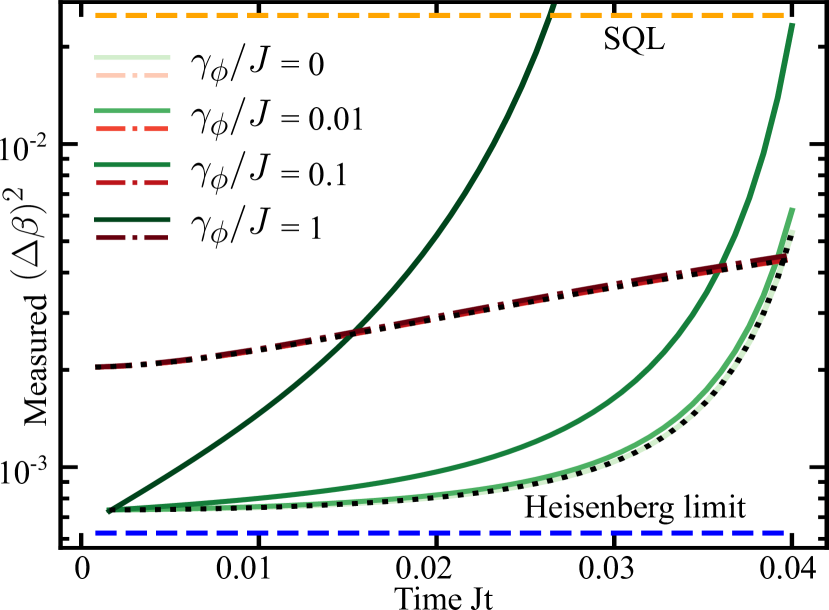
Figure 2: Measured $(\Delta\beta)^{2}$ as a function of dimensionless signal acquisition time $Jt$ by evolving the optimal state minimising $(\Delta\beta)^{2}$ under a field coupled with the spins with coupling strength $J$ with local homogeneous dephasing acting on the spins with rates $\gamma_{\phi}/J=0,0.01,0.1,1.0$ for $N=40$, $C=10^{4}$, $\gamma/\kappa=1.0$. Green solid lines (darker shade for larger $\gamma_{\phi}$) correspond to GHZ-like states while red dash-dot lines correspond to the $\ket{\mathcal{D}^{N}_{N/2}}$-like states. Dotted black curves are the optimal $(\Delta\beta)^{2}$ obtained with analytic solution of $\mathcal{E}_{\mathrm{gpg}}$ for $\gamma_{\phi}/J=0$.

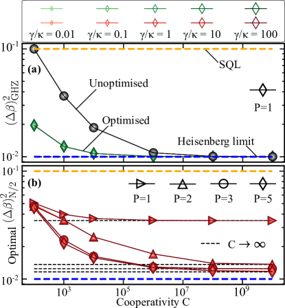
Figure S1: (a) Optimal $(\Delta\beta)^{2}_{\mathrm{GHZ}}$ for $P=1$ step obtained as a function of Cooperativity $C$ , plotted for $N=10$ and different ratios $\gamma/\kappa$. The circle markers correspond to the results obtained with the application of unoptimised pulses referring to the pulses which prepare the ideal GHZ state with $(\Delta\beta)^{2}_{\mathrm{GHZ}}=1/N^{2}$ for the case $\kappa=\gamma=0$. (b) $(\Delta\beta)^{2}_{N/2}$ for $P=1,2,3,5$ steps obtained as a function of Cooperativity $C$ , plotted for $N=10$ and different ratios $\gamma/\kappa$.

We perform extensive numerical simulations in the parameter ranges $10\leq N\leq 100$, $25\leq C\leq 10^{6}$, $10^{-2}\leq\gamma/\kappa\leq 10^{2}$ for cavity pulse durations $10\leq gT\leq 10^{2}$. For both cases (I) and (II), we find that the noise-informed protocol prepares final probe states resulting in measurement variances $(\Delta\beta)^{2}$ that scale better with $N$ than the SQL in all cases with $C\gtrsim 20$ and closely approach the Heisenberg scaling $(\Delta\beta)^{2}\sim N^{-2}$ for $C\gtrsim 10^{3}$, independently of the ratio $\gamma/\kappa$. Pulse durations $gT\lesssim 40$ are sufficient to converge to analytic results obtained in the adiabatic limit $gT\rightarrow\infty$ from Eqs. (2) and (5), in all shown cases. For each $N$ and $\gamma/\kappa$, $(\Delta\beta)^{2}$ decreases monotonically with increasing $P$, reaching the analytic predictions for $C\rightarrow\infty$ in just a few steps (see Fig. S1 in Supplemental Material). The resulting global control pulses have a smooth, continuous form for all protocol steps $P$.

Figure 1(b1) and (b2) show example results of optimal cavity drive pulses $\eta(t)$ found to minimize $(\Delta\beta)^{2}$ for observables (I) and (II), respectively, for $N=40$, $C=10^{4}$, $\gamma/\kappa=0.01$ and $gT=40$. The plots show a continuous, smooth profile for both real and imaginary parts of $\eta(t)$. Surprisingly, the protocol requires only $P=1$ and $P=3$ steps to reach converge to the asymptotic results with $P\rightarrow\infty$ for cases (I) and (II), respectively. For each $P$, panels (c1) and (c2) show the corresponding state trajectories in Husimi-Q representation of qubit state in the symmetric Dicke subspace. As expected, they appear similar, but not identical, to those of GHZ and symmetric Dicke states: asymmetries due to squeezing-like behavior are visible, resulting on only $\sim 57\%$ and $\sim 15\%$ overlap with ideal GHZ and symmetric Dicke states, respectively. Nevertheless, we term them as GHZ-like and $\ket{\mathcal{D}^{N}_{N/2}}$-like states. Panels (d) and (e) summarize our results for optimal $(\Delta\beta)^{2}$ as a function of qubit number $N$, for different cooperativities $C$ and linewidth ratios $\gamma/\kappa$, computed in the limit $gT\rightarrow\infty$. For each $N$, $C$ and $\gamma/\kappa$, the optimisation is performed $\mathcal{O}(N)$ times with randomly initialised parameters and the best value is plotted. For case (I) [panel (d)], the optimal probe states prepared with the noise-informed protocol surpass the SQL with variance $(\Delta\beta)^{2}_{\mathrm{GHZ}}$ scaling with $N$ as $\sim N^{-1.24}$ for cooperativities as small as $C=25$, as $\sim N^{-1.52}$ for $C=100$, and closely approaching the Heisenberg limit for $C\gtrsim 10^{4}$, with scaling $\Delta\beta^{2}\sim N^{-\alpha}$ and $\alpha>1.93$. For case (II) [panel (e)], the optimal $(\Delta\beta)^{2}_{N/2}\sim N^{-\alpha}$ scale with $\alpha\approx 1.4$ for $C=25$, $\alpha\approx 1.5$ for $C=10^{2},10^{4}$ and $\alpha\approx 1.6$ for $C=10^{6}$, showing considerable improvement over the SQL for all $C$. In all cases, optimal results are essentially independent of the ratio $\gamma/\kappa$. While our sensing protocol does not allow for arbitrarily high precision, i.e. arbitrarily large $N$, as to be expected since no QEC is employed, it provides a simple method using minimal quantum control resources to achieve quantum advantage in the presence of realistic noise.

In order to explore the experimental observability of the above predictions, in Fig. 2 we show the performance of the prepared optimal probe states during signal collection in a field-sensing experiment where spin qubits are additionally subjected to local dephasing with rate $\gamma_{\phi}$, as originated for example by optical trapping of atoms in independent tweezers [26]. Homogeneous local dephasing can be described as a collective process [27], with each $N$-qubit state $\rho$ in the collective Hilbert space $\mathcal{H}_{C}$ of dimension $\sum_{J=J_{\mathrm{min}}}^{J_{\mathrm{max}}}(2J+1)$, with $J_{\mathrm{max}}=N/2$ and $J_{\mathrm{min}}=(N$ mod $2)/2$. Having the field generator $\hat{H}_{\vec{n}}$, we describe the homogeneous local dephasing (fluctuations in transition frequency) with rate $\gamma_{\phi}$ on the two-level spin with index ’$j$’ using the jump operator $\mathcal{A}^{(j)}=\frac{1}{2}\hat{\sigma}_{z}^{(j)}$ where $\hat{\sigma}_{z}^{(j)}=|1_{j}\rangle\langle 1_{j}|-|0_{j}\rangle\langle 0_{j}|$. The optimal probe state $\rho_{\mathrm{opt}}$ evolves according to $\dot{\rho}_{\mathrm{opt}}=-i\left[\hat{H}_{\vec{n}},\rho_{\mathrm{opt}}\right]+\gamma_{\phi}\sum_{j=1}^{N}\mathcal{L}^{(j)}[\rho_{\mathrm{opt}}]$, where $\mathcal{L}^{(j)}[\rho_{\mathrm{opt}}]=\mathcal{A}^{(j)}\rho_{\mathrm{opt}}(\mathcal{A}^{(j)})^{\dagger}-\frac{1}{2}\{(\mathcal{A}^{(j)})^{\dagger}\mathcal{A}^{(j)},\rho_{\mathrm{opt}}\}$. We solve the model numerically using piqs package [28], using optimal probe states prepared for $N=40$, $C=10^{4}$ and $\gamma/\kappa=1.0$ as initial state at $Jt=0$. Figure 2 shows that $(\Delta\beta)^{2}_{\mathrm{GHZ}}$ increases rapidly with time $t$ as $\sim e^{N\gamma_{\phi}t}$ for any given $\gamma_{\phi}/J$ using GHZ-like probe states[29, 30]. Results for $\ket{\mathcal{D}^{N}_{N/2}}-$like states appear instead to be essentially independent of $\gamma_{\phi}/J$ for the shown $t$[29](see also Supplemental Material for results with dephasing added during state preparation). Our results are directly relevant to state-of-the-art experiments with neutral atoms trapped in optical cavities. As an example, we consider ⁸⁷Rb atoms trapped in optical tweezers and coupled to a fiber Fabry-Perot cavity [31, 32, 33]. We choose qubit states $\ket{0}=\ket{5^{2}S_{1/2},F=1,m_{F}=0}$, $\ket{1}=\ket{5^{2}S_{1/2},F=2,m_{F}=0}$, and $\ket{e}=\ket{5^{2}P_{3/2},F=3,m_{F}=0}$, where the linewidth of the $\ket{1}\leftrightarrow\ket{e}$ transition ($\lambda=780\,$nm) is $\gamma=2\pi\times 6\,$MHz (FWHM). We assume a cavity finesse $F\approx 2\times 10^{5}$, a waist radius $\omega_{0}\approx 2\,\mu$m and a length $L\approx 40\,\mu$m resulting in a cooperativity of $C=3\lambda^{2}F/(2\pi^{3}\omega_{0}^{2})\approx 1500$ with a coupling strength of $g=\sqrt{3\lambda^{2}C\gamma}/(2\pi^{2}\omega_{0}^{2}L)\approx 2\pi\times 400\,$MHz and $\kappa=\pi C/LF\approx 2\pi\times 20\,$MHz (FWHM), so that $\gamma/\kappa\approx 0.3$. Our noise-informed state preparation protocol obtains for $N=10$ atoms a minimal $(\Delta\beta)^{2}_{N/2}=0.022$ with $P=3$ protocol steps and a minimal $(\Delta\beta)^{2}_{\mathrm{GHZ}}=0.013$ with $P=1$ protocol step, where in each step the cavity pulse is applied for a duration $T=20g^{-1}\approx 8\,$ns. Tweezer induced dephasing rates on state $\ket{1}$ can be as small as $\gamma_{\phi}/g=0.03\times 10^{-6}$ [34], which we find to be negligible (see also Supplemental Material).

Finally we note that, beyond the preparation of metrological states presented here, the setup described above is sufficient to achieve unitary synthesis in the Dicke subspace. In fact, the control algebra $\{\hat{J}_{z}^{2},\hat{J}_{x},\hat{J}_{y},\hat{J}_{z}\}$ used above is universal for Dicke state preparation starting from a canonical product state like $\ket{D^{N}_{N}}$ [16, 17]. In the companion work Ref. [12] we propose an alternative adiabatic phase gate using the same cavity setup as above but in the weak drive, long pulse time limit with detunings $\Delta,\delta=O(g)$. There we show that sequential application of $N$ adiabatic gates can generate a multi-controlled phase gate deterministically $V(\phi)=e^{i\phi\ket{D^{N}_{N}}\bra{D^{N}_{N}}}$. Writing an arbitrary unitary in the Dicke subspace in its spectral decomposition, $U=\sum_{j=1}^{N+1}e^{i\lambda_{j}\ket{\lambda_{j}}\bra{\lambda_{j}}}$, the following decomposition suffices $U=\prod_{j=1}^{N+1}W(\lambda_{j})^{\dagger}V(\lambda_{j})W(\lambda_{j})$, where $W(\lambda_{j})^{\dagger}$ is any unitary extension of the state mapping $W(\lambda_{j})^{\dagger}\ket{D^{N}_{N}}=\ket{\lambda_{j}}$.

While the results presented in this work are directly relevant to state-of-the-art experiments with cold atoms trapped in tweezer arrays in cavities as shown above, we anticipate that our noise-informed protocols can be generalized to different physical setups and noise models, e.g. for Rydberg atoms and cold ion chains. This will be subject of future work.

Supplemental Material

I Exact solution of the geometric phases in the presence of losses

In this section, we present the exact solution of the geometric phases $\varphi_{nm}(T)$ in Eq. 2 (of the main text).

We describe the state of the joint spin-cavity system at any time $t$ as $\rho(t)=\sum_{n,m}\rho_{nm}(t)$, and use an Ansatz for the state components $\rho_{nm}(t)$ given by

$$\rho_{nm}(t)=e^{i\varphi_{nm}(t)}\ket{\beta_{n}}\bra{\beta_{m}}\otimes\ket{q_{n}}\bra{q_{m}}/\langle\beta_{n}|\beta_{m}\rangle,$$ (S1)

where $\varphi_{nm}(t)$ are the geometric-phases acquired by the qubit state component $\ket{q_{n}}\bra{q_{m}}$, and $\ket{\beta_{n}}\bra{\beta_{m}}$ is the corresponding state of the cavity mode. With this Ansatz, we exactly solve the open quantum system for $\rho_{nm}(t)$ with $\kappa,\gamma\neq 0$. The later is described by the Lindbladian master equation given by

$$\dot{\rho}_{nm} =-i\hat{H}_{\mathrm{eff}}^{n}\rho_{nm}+i\rho_{nm}(\hat{H}_{\mathrm{eff}}^{m})^{{\dagger}}+\hat{L}\rho_{nm}\hat{L}^{{\dagger}}-\frac{1}{2}\{\hat{L}^{{\dagger}}\hat{L},\rho_{nm}\},$$

with $\hat{H}_{\mathrm{eff}}^{n}=\delta a^{{\dagger}}a+(-i\frac{\gamma_{1}}{2}+\zeta(t)\hat{a}^{{\dagger}}+\zeta(t)^{*}\hat{a})n$. On substituting the Ansatz for $\rho_{nm}$ in the master equation, we obtain the derivatives for $\beta_{n}(t)$ and $\varphi_{nm}(t)$ as(see Ref. [12]),

$$\dot{\beta}_{n} = -(i\delta+\kappa/2)\beta_{n}-in\zeta,$$ (S2)

$$\dot{\varphi}_{nm} = (m-n)(\zeta\beta_{m}+\zeta^{*}\beta_{n})+i(m+n)\gamma_{1}/2.$$ (S3)

We now take the initial state of the joint spin-cavity system as $\rho(0)=\ket{\beta_{n}(0)}\bra{\beta_{m}(0)}\otimes\ket{q_{n}}\bra{q_{m}}$, which forms the basis for all possible initial states and is hence sufficient to obtain a general solution for the state evolution. The solutions corresponding to $\beta(t)$ and $\psi_{nm}(t)$ are then given by

$$\beta_{n}(t)=\beta_{n}(0)e^{-(i\delta+\kappa/2)t}-in\int_{0}^{t}\mathrm{d}t^{\prime}\zeta(t^{\prime})e^{-(i\delta+\kappa/2)(t-t^{\prime})},$$ (S4)

and

$$\varphi_{nm}(t)=\int_{0}^{t} \Big{[} (m-n)(\zeta(t)\beta_{m}(t)^{*}+\zeta(t)^{*}\beta_{n}(t))$$ (S5)

$$+ i(m+n)\gamma_{1}(t)/2\Big{]}\mathrm{d}t.$$

The cavity drive pulses $\zeta(t)$ in $\hat{H}_{\mathrm{eff}}$ are chosen of duration $T$ such that $\zeta(0)=\zeta(T)=0$ so that $\beta_{n}(0)=\beta_{n}(T)$, ensuring that the cavity mode is decoupled from the spins at the end of the geometric phase gate. One can hence write the corresponding quantum channel of the geometric phase gate on a spin basis state by tracing out the cavity mode as in Eq. (2).

II Optimal state-preparation-protocol at $gT\rightarrow\infty$ and at finite $gT$

In this section, we discuss the numerical optimisation details for both the cases of the cavity pulse duration in the application of $\mathcal{E}_{\mathrm{gpg}}$ corresponding to $gT\rightarrow\infty$ and for a finite $gT$.

For finding the optimal state preparation protocol parameters for the case of $gT\rightarrow\infty$, we make use of Eq. (5)(in the main text) in the application of $\mathcal{E}_{\mathrm{gpg}}$ where we have $\phi=\frac{1}{\delta}\int_{0}^{T}|\zeta(t)|^{2}$, and hence we must have the same sign for $\phi_{j}$ and $\delta_{j}$ in each step $j$ while finding the optimal parameters. We hence perform a boundless optimisation using $\varphi_{nm}=(n^{2}-m^{2})\phi_{j}+(m-n)^{2}\frac{i\kappa}{2}\left|\frac{\phi_{j}}{\delta_{j}}\right|+(m+n)\frac{i\gamma}{2g^{2}}\left|\phi_{j}\delta_{j}\right|$, and post adjust the sign of $\delta_{j}$ corresponding to the sign of $\phi_{j}$.

For finding the optimal protocol parameters for a finite cavity pulse duration, the quantum channel $\mathcal{E}_{\mathrm{gpg}}$ from Eq. 2 is applied using the solution in Eqs.S4- S5 with $\beta_{n}(0)=0$, that is assuming the cavity mode starts in vacuum(note that the protocol is independent of the initial cavity state, see Ref. [12]). The optimisation is partially bounded where the bounds are introduced for the $\delta_{j}$ values arising from the physical constraint of limiting the pulse duration to $gT$ while keeping reasonable $\mathrm{max}_{t}|\eta(t)|$. The constraint can be explicitly written from the transformation from the full Hamiltonian to the effective Hamiltonian in Eq. (1), as $|\zeta|^{2}<g^{2}/4$, which sets the bounds $\delta^{(j)}\in\left(\frac{2\pi}{T},\frac{3g^{2}T}{32\phi^{(j)}}\right)$. We start the optimisation with the parameters corresponding to the $T\rightarrow\infty$ case, with $\delta^{(j)}$s adjusted within the bounds mentioned above. Fig.S2 shows the obtained optimal $(\Delta\beta)^{2}_{\mathrm{GHZ}}$ and $(\Delta\beta)^{2}_{N/2}$ as a function of the cavity pulse duration in each application of $\mathcal{E}_{\mathrm{gpg}}$. The obtained optimal values optimal $(\Delta\beta)^{2}_{\mathrm{GHZ}}$ and $(\Delta\beta)^{2}_{N/2}$ show a dependence on $\gamma/\kappa$ and is minimal for $\gamma=\kappa$. For large cooperativities of $C>100$, the optimal values converge close to the values corresponding to $gT\rightarrow\infty$ case for pulse durations $gT\approx 30-40g^{-1}$.

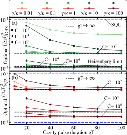
Figure S2: (a) Optimal $(\Delta\beta)^{2}_{GHZ}$ for $P=1$ step and (b) $(\Delta\beta)^{2}_{N/2}$ for $P=3$ steps obtained as a function of the cavity drive pulse duration $gT$, plotted for $N=10$, cooperativities $C=10^{2},10^{4},10^{6}$ and different ratios $\gamma/\kappa$.

III Exact derivatives of the protocol cost function

In this section we provide the derivatives of our protocol cost function $(\Delta\beta)^{2}$ with respect to all parameters $\Theta=\{\theta^{\alpha}_{0},\theta^{\beta}_{0},\theta^{\gamma}_{0},\theta^{\alpha}_{j},\theta^{\beta}_{j},\theta^{\gamma}_{j},\phi_{j},\delta_{j}\dots\forall j=1,2\dots P\}$. We first start out by writing the derivatives of the states obtained after each protocol step.

Our protocol starts with the application of $\hat{\mathcal{U}}_{0}$ on the initial state $\rho_{\mathrm{in}}=\ket{\mathcal{D}_{0}}$, giving $\rho_{0}=\hat{\mathcal{U}}_{0}\rho_{\mathrm{in}}\hat{\mathcal{U}}_{0}^{\dagger}$. The states $\rho_{j}$ obtained after application of protocol step $j$ for $j=1,2\dots P$ are obtained as

$$\rho_{j} = \hat{\mathcal{U}}_{j}\mathcal{E}_{gpg}(\rho_{j-1})\hat{\mathcal{U}}_{j}^{\dagger}.$$ (S6)

It is then straightforward to write the derivatives of $\rho_{0}$ and $\rho_{j}$ $\forall j=1,2,\dots P$ with respect to the parameters $\Theta$, which are obtained as given below

$$\partial_{\theta_{0}}\rho_{0} =(\partial_{\theta_{0}}\hat{U}_{0})\rho_{\mathrm{in}}\hat{U}_{0}^{\dagger}+\hat{U}_{0}\rho_{\mathrm{in}}(\partial_{\theta_{0}^{\alpha}}\hat{U}_{0}^{\dagger}),$$

$$\partial_{\theta_{j}}\rho_{0} =\partial_{\phi_{j}}\rho_{0}=\partial_{\delta_{j}}\rho_{0}=0,$$

$$\partial_{\theta_{j}}\rho_{j} =(\partial_{\theta_{j}}\hat{U}_{j})\mathcal{E}_{gpg}(\rho_{j-1})\hat{U}_{j}^{\dagger}+\hat{U}_{j}\mathcal{E}_{gpg}(\rho_{j-1})(\partial_{\theta_{j}}\hat{U}_{j}^{\dagger}),$$

$$\partial_{\phi_{j}}\rho_{j} =\hat{U}_{j}(\sum_{n,m}\partial_{\phi_{j}}(\varphi_{nm})e^{i\varphi_{nm}}\bra{\mathcal{D}_{n}}\rho_{j}\ket{\mathcal{D}_{m}}\ket{\mathcal{D}_{n}}\bra{\mathcal{D}_{m}})\hat{U}_{j}^{\dagger},$$

$$\partial_{\delta_{j}}\rho_{j} =\hat{U}_{j}(\sum_{n,m}\partial_{\delta_{j}}(\varphi_{nm})e^{i\varphi_{nm}}\bra{\mathcal{D}_{n}}\rho_{j}\ket{\mathcal{D}_{m}}\ket{\mathcal{D}_{n}}\bra{\mathcal{D}_{m}})\hat{U}_{j}^{\dagger}$$

$$\partial_{\Theta_{k<j}}\rho_{j} =\mathcal{E}_{j}\dots\mathcal{E}_{k+1}(\partial_{\Theta_{k}}\rho_{k}),\partial_{\Theta_{k>j}}\rho_{j}=0.$$

We have used the shorthand $\theta_{j}$ for $\theta_{j}^{\alpha},\theta_{j}^{\beta},\theta_{j}^{\gamma}$ and $\Theta_{j}$ refers to all elements in the set $\{\theta_{j}^{\alpha},\theta_{j}^{\beta},\theta_{j}^{\gamma},\phi_{j},\delta_{j}\}$ in the equations above. Note that the derivatives of the state $\rho_{j}$ are simply obtained by performing similar operations- applying the geometric-phase-gate operation $\mathcal{E}_{\mathrm{gpg}}$ and global spin rotation operations. For example, obtaining $\partial_{\phi_{j}}\rho_{j}$ and $\partial_{\delta_{j}}\rho_{j}$ are similar to calculating $\mathcal{E}_{\mathrm{gpg}}(\rho_{j})$ but with modified phases $e^{i\varphi_{nm}}\rightarrow\partial_{\phi_{j}}(\varphi_{nm})e^{i\varphi_{nm}}$ and $e^{i\varphi_{nm}}\rightarrow\partial_{\delta_{j}}(\varphi_{nm})e^{i\varphi_{nm}}$ respectively. The optimal probe state is prepared after at $j=P$ protocol steps which we denote by $\rho_{P}=\rho_{\mathrm{opt}}$. With the prescription described above we obtain the exact derivatives corresponding to $\partial_{\Theta}\rho_{\mathrm{opt}}$, for all parameters $\Theta$. In the following, we obtain the derivatives of the protocol cost function $(\Delta\beta)^{2}$ for the two choices of the measurement operator $\hat{M}$ corresponding to $(\Delta\beta)^{2}_{\mathrm{GHZ}}$ and $(\Delta\beta)^{2}_{N/2}$ for case I and II below respectively.

III.0.1 Case I: Choosing $\hat{M}=\hat{\mathcal{P}}_{x}=\bigotimes_{i=1}^{N}\hat{\sigma}_{x}^{(i)}$

The operator $\mathcal{P}_{x}=\bigotimes_{i=1}^{N}\hat{\sigma}_{x}^{(i)}$ measures the parity of the state along $x$. Using $e^{i\pi/2\sigma_{x}}=i\sigma_{x}$, we rewrite $\hat{M}$ as

$$\hat{M} = e^{i\pi(\hat{J}_{x}-N/2)}.$$ (S7)

We choose the field generator corresponding to a field along $z$ for this case as $\hat{H}_{\vec{z}}=J\hat{J}_{z}$. Let the state obtained after the rotation of the optimal probe state $\rho_{\mathrm{opt}}$ by an angle $\beta=Jt$ along the field axis be denoted by $\rho_{\mathrm{opt}}^{\beta}$. We obtain

$$\rho_{\mathrm{opt}}^{\beta}=e^{-i\beta\hat{J}_{z}}\rho_{\mathrm{opt}}e^{i\beta\hat{J}_{z}},\hskip 1.00006pt\partial_{\beta}\rho_{\mathrm{opt}}^{\beta}=i\left[\rho_{\mathrm{opt}}^{\beta},\hat{J}_{z}\right],$$ (S8)

$$\partial_{\Theta}\partial_{\beta}\rho_{\mathrm{opt}}^{\beta}=i\left[\partial_{\Theta}\rho_{\mathrm{opt}}^{\beta},\hat{J}_{z}\right],$$ (S9)

$$\langle\hat{\mathcal{P}}_{x}(\beta)\rangle=\mathrm{Tr}(\hat{\mathcal{P}}_{x},\rho_{\mathrm{opt}}^{\beta}),$$ (S10)

$$\partial_{\Theta}\langle\hat{\mathcal{P}}_{x}(\beta)\rangle=\mathrm{Tr}(\hat{\mathcal{P}}_{x},\partial_{\Theta}\rho_{\mathrm{opt}}^{\beta}),$$ (S11)

where $\partial_{\Theta}\rho_{\mathrm{opt}}^{\beta}=e^{-i\beta\hat{J}_{z}}(\partial_{\Theta}\rho_{\mathrm{opt}})e^{i\beta\hat{J}_{z}}$. Similarly, $\langle\hat{\mathcal{P}}_{x}^{2}(\beta)\rangle=\mathrm{Tr}(\hat{\mathcal{P}}_{x}^{2},\rho_{\mathrm{opt}}^{\beta})$, $\partial_{\Theta}\langle\hat{\mathcal{P}}^{2}_{x}(\beta)\rangle=\mathrm{Tr}(\hat{\mathcal{P}}^{2}_{x},\partial_{\Theta}\rho_{\mathrm{opt}}^{\beta})$, $\partial_{\beta}\langle\hat{\mathcal{P}}_{x}(\beta)\rangle=\mathrm{Tr}(\hat{\mathcal{P}}_{x},\partial_{\beta}\rho_{\mathrm{opt}}^{\beta})$ and $\partial_{\Theta}\partial_{\beta}\langle\hat{\mathcal{P}}_{x}(\beta)\rangle=\mathrm{Tr}(\hat{\mathcal{P}}_{x},\partial_{\Theta}\partial_{\beta}\rho_{\mathrm{opt}}^{\beta})$.

With these, we obtain the derivatives of $(\Delta\beta)^{2}_{\mathrm{GHZ}}$ as

$$\partial_{\Theta}(\Delta\beta)^{2}_{\mathrm{GHZ}}=\left[\left(\partial_{\Theta}\langle\hat{\mathcal{P}}^{2}_{x}(\beta)\rangle-\partial_{\Theta}(\langle\hat{\mathcal{P}}_{x}(\beta)\rangle)^{2}\right)\left|\partial_{\beta}\langle\hat{\mathcal{P}}_{x}(\beta)\rangle\right|^{2}\right.$$

$$\left.-\left(\langle\hat{\mathcal{P}}^{2}_{x}(\beta)\rangle-\langle\hat{\mathcal{P}}_{x}(\beta)\rangle^{2}\right)\partial_{\Theta}\left|\partial_{\beta}\langle\hat{\mathcal{P}}_{x}(\beta)\rangle\right|^{2}\right]/\left|\partial_{\beta}\langle\hat{\mathcal{P}}_{x}(\beta)\rangle\right|^{4}.$$ (S12)

III.0.2 Case II: Choosing $\hat{M}=\hat{J}_{z}^{2}$

For this choice of measurement operator $\hat{M}$, we choose the field along $y$ axis corresponding to $\hat{H}_{\vec{y}}=J\hat{J}_{y}$. The second and the fourth moments for $\hat{M}=\hat{J}_{z}^{2}$ after rotation of the probe state $\rho_{\mathrm{opt}}$ by angle $\beta=Jt$, written with $\langle\hat{X}\rangle=\mathrm{Tr}(\hat{X},\rho_{\mathrm{opt}})$ are given by

$$\langle{\hat{J}_{z}^{2}(\beta)}\rangle =\langle{\hat{J}_{z}^{2}}\rangle\cos^{2}{\beta}+\langle{\hat{J}_{x}^{2}}\rangle\sin^{2}{\beta}-\langle{\{{\hat{J}_{z}},{\hat{J}_{x}}\}}\rangle\sin{\beta}\cos{\beta},$$ (S13)

$$\langle{\hat{J}_{z}^{4}(\beta)}\rangle =\langle{\hat{J}_{z}^{4}}\rangle\cos^{4}{\beta}+\langle{\hat{J}_{x}^{4}}\rangle\sin^{4}{\beta}$$ (S14)

$$+(\langle{\{{\hat{J}_{z}},{\hat{J}_{x}}\}^{2}}\rangle+\langle{\{{\hat{J}_{z}^{2}},{\hat{J}_{x}^{2}}\}}\rangle)\cos^{2}{\beta}\sin^{2}{\beta}$$

$$-\langle{\hat{A}}\rangle\cos^{3}{\beta}\sin{\beta}-\langle{\hat{B}}\rangle\cos{\beta}\sin^{3}{\beta},$$

where $\hat{A}=\{{\hat{J}_{z}^{2}},{\{{\hat{J}_{z}},{\hat{J}_{x}}\}}\}$ and $\hat{B}=\{{\hat{J}_{x}^{2}},{\{{\hat{J}_{z}},{\hat{J}_{x}}\}}\}$.

The variance of the measurement results is then obtained as $(\Delta\hat{J}_{z}^{2}(\beta))^{2}=\langle{\hat{J}_{z}^{4}(\beta)}\rangle-\langle{\hat{J}_{z}^{2}(\beta)}\rangle^{2}$. The derivative term in the denominator of $(\Delta\beta)^{2}$ is obtained as

$$\partial_{\beta}\langle{\hat{J}_{z}^{2}(\beta)}\rangle =2(\langle{\hat{J}_{x}^{2}}\rangle-\langle{\hat{J}_{z}^{2}}\rangle)\cos{\beta}\sin{\beta}$$ (S15)

$$-\langle{\{{\hat{J}_{z}},{\hat{J}_{x}}\}}\rangle(\cos^{2}{\beta}-\sin^{2}{\beta}).$$

By writing $\partial_{\Theta}\langle\hat{X}\rangle=\mathrm{Tr}(\hat{X},\partial_{\Theta}\rho_{\mathrm{opt}})$, it is straightforward to obtain $\partial_{\Theta}(\Delta\beta)^{2}_{N/2}$ similar to Eq. (III.0.1).

IV Optimal state preparation protocol parameters

In this section, we tabulate the obtained optimal parameters $\Theta$ in $\mathcal{E}_{q}$ which prepare the optimal probe states $\rho_{\mathrm{opt}}$ minimising $(\Delta\beta)^{2}_{\mathrm{GHZ}}$ and $(\Delta\beta)^{2}_{N/2}$ in Tables 1 and 2 respectively.

$N$	$C$	$\gamma/\kappa$	$N(\Delta\beta)^{2}_{\mathrm{GHZ}}$	$(\theta_{0}^{\alpha},\theta_{0}^{\beta},\theta_{0}^{\gamma})$
				$(\phi_{1},\delta_{1},\theta_{1}^{\alpha},\theta_{1}^{\beta},\theta_{1}^{\gamma})$, $\Delta_{1}$
10	$10^{2}$	0.01	0.61	(0.98, 1.57, 0.88)
				(0.86, 2.18g, -1.16, 1.57, 0.96), 26g
		1.0	0.20	(1.57, 1.41, 0.34)
				(1.56, 0.48g, 0, 1.57, 1.36), 237g
	$10^{4}$	0.01	0.109	(0, 1.56, 0.50)
				(1.56, 2.15g, 0, 1.57, -0.04), 9g
		1.0	0.107	(-0.22, 1.55, 0.36)
				(1.57, 0.44g,0, 1.57, 0.19), 267g
40	$10^{2}$	1.0	0.096	(-0.34, 1.14, 0.50)
				(1.61, 0.30g, 0, 1.57, 0.07), 457g
	$10^{4}$	0.01	0.030	(1.51, 1.54, 0.37)
				(1.57, 2.03g , 0.08, 1.57, 1.58), 12g
		1.0	0.029	(-0.04, 1.53, 0.37)
				(1.57, 0.28g, 0.08, 1.57,0.02), 497g
100	$10^{2}$	0.01	0.15	(1.51, 0.98, 0.69)
				(1.56, 2.13g, 0, 1.57, 1.32), 10g
		1.0	0.07	(1.47, 0.87, 0.69)
				(1.64, 0.24g, 0, 1.57, 1.29), 597g
	$10^{4}$	0.01	0.013	(1.42, 1.51, 0.22)
				(1.57, 1.80g, 0.03, 1.57, 1.66 ), 19g
		1.0	0.013	(1.38, 1.51, 0.22)
				(1.57, 0.18g, 0.03, 1.57, 1.63), 844g

Table 1: Optimal state preparation protocol parameters $\Theta_{\mathrm{opt}}$ minimizing $(\Delta\beta)^{2}_{\mathrm{GHZ}}$. The listed values correspond to the cavity pulses in the application of geometric phase gate $\mathcal{E}_{\mathrm{gpg}}$ of duration of $T=40g^{-1}$. The $\Delta_{j}$ values are derived from the optimal $\phi_{j}$, $\delta_{j}$ and the choice of $\mathrm{max}_{t}(|\eta(t)|)=30g$ by inverting the pulse $\zeta(t)$ in Eq. (1) to $\eta(t)$ in the full Hamiltonian. An extra rotation along $\hat{z}$ direction to set $\beta_{\mathrm{opt}}=0$ is incorporated in $\theta^{\alpha}_{1}$[19].

$N$	$C$	$\gamma/\kappa$	$N(\Delta\beta)^{2}_{N/2}$	$(\theta_{0}^{\alpha},\theta_{0}^{\beta},\theta_{0}^{\gamma})$, $\theta_{-1}^{\beta}$
				$(\phi_{1},\delta_{1},\theta_{1}^{\alpha},\theta_{1}^{\beta},\theta_{1}^{\gamma})$, $\Delta_{1}$
				$(\phi_{2},\delta_{2},\theta_{2}^{\alpha},\theta_{2}^{\beta},\theta_{2}^{\gamma})$, $\Delta_{2}$
				$(\phi_{3},\delta_{3},\theta_{3}^{\alpha},\theta_{3}^{\beta},\theta_{3}^{\gamma})$, $\Delta_{3}$
10	$10^{2}$	0.01	0.51	(1.19, 2.10, 0.66), 2.22
				(0, -, -2.11, 1.50, 0.70), -
				(0.21, 8g, -2.46, 2.15, -1.72), 8g
				(0.02, 7.06g, -0.96, 2.86, -2.01), 39g
		1.0	0.47	(1.15, -0.97, 0.43), 0.24
				(0.08, 1.17g, 0.49, 1.08, 0.92), 323g
				(-0.14, -0.83g, -0.25, 0.96, 0.92), 393g
				(0.06, 1.06g, -0.99, -0.59, 0.13), 427g
	$10^{4}$	0.01	0.165	(-0.08, -1.57, 0.63), 0.09
				(0.10, 7.22g, 0.29, 2.52, -0.48), 17g
				(0.30, 5.66g, 1.91, 0.18, -0.42), 11g
				(1.38, 1.86g, 0.92, 0, 1.57), 21g
		1.0	0.163	(-0.34, 1.57, 0.42), 2.09
				(0.10, 1.14g, 1.68, 0.61, -0.23), 293g
				(0.29, 0.67g, 0.49, 0.18, 1.25), 362g
				(1.38, 0.25g, 3.14, 2.00, 0.79), 611g
40	$10^{2}$	0.01	0.21	(0.04, 0, 0.41), -0.03
				(0.95, 0.41g, -1.03, 1.51, 0.43), 265g
				(-0.07, -7.07g, -2.59, 0.63, -0.19), 21g
				(0.03, 7.07g, 1.82, -0.26,-2.74 ), 33g
		1.0	0.20	(0.36, -1.51, 0.49), -1.08
				(0.06, 0.82g, -0.90, 2.47, 0.45), 600g
				(-0.04, -0.71g, -0.41, 0.56, -0.84), 900g
				(0.01, 0.94g, 0.33, 1.16, -0.90), 1200g
	$10^{4}$	0.01	0.081	(0.29, 1.57, 0.74), 0.51
				(0.05, 6.34g, 1.50, 0.42, -0.02), 32g
				(0.22, 5.72g, -0.35, 0.09, 0.97), 15g
				(1.47, 0.89g, 0, 0.48, -0.60), 90g
		1.0	0.086	(0.26, 1.57, 0.74), 0.51
				(0.04, 5.30g, 1.28, 0.43, -0.05), 44g
				(0.21, 0.67g, -0.67, 0.09, 0.75), 400g
				(1.45, 0.17g, 0, -0.48, -0.92), 900g
100	$10^{2}$	0.01	0.133	(0.23, 0, 0.72), 2.16
				(0.32, 0.64g, -1.93, -1.58, 0.92), 300g
				(-0.04, -7.07g, 1.83, -0.34, -1.05), 28g
				(0.04, 3.26g, -0.11, 0.97, 1.33), 90g
	$10^{4}$	0.01	0.045	(-1.17, 1.55, 0.53), 0
				(0.02, 15.69g, 0.078, -0.34, -1.07), 11g
				(0.17, 4.55g, 0.84, 0.10, 0.80), 26g
				(-0.08, -7.07g, 1.07, 0.04, 0.88), 19g
		1.0	0.048	(0.49, 1.59, 0.71), -0.07
				(0.03, 0.76g, -0.08, 0.32, 0.85), 1000g
				(0.18, 0.25g, 0.26, 0.05, 0.33), 1800g
				(0.43, 0.17g, 0.21, 0.08, 0.75), 1700g

Table 2: Optimal state preparation protocol parameters $\Theta_{\mathrm{opt}}$ minimizing $(\Delta\beta)^{2}_{N/2}$. The listed values correspond to the cavity pulses in the application of geometric phase gate $\mathcal{E}_{\mathrm{gpg}}$ of duration of $T=40g^{-1}$.The $\Delta_{j}$ values are derived from the optimal $\phi_{j}$, $\delta_{j}$ and the choice of $\mathrm{max}_{t}(|\eta(t)|)=30g$ by inverting the pulse $\zeta(t)$ in Eq. (1) to $\eta(t)$ in the full Hamiltonian. The angles $\theta_{-1}^{\beta}$ refer to the extra rotation along the field axis $\hat{y}$ at the end of the protocol steps to set $\beta_{\mathrm{opt}}=0$ [19].

V Spins under local homogeneous dephasing during state preparation

In this section, we study the robustness of our state preparation protocol against the local homogeneous dephasing process. We consider the dephasing effects introduced as local homogeneous dephasing processes, which can be described as a collective process[27], and we work in the collective Hilbert space $\mathcal{H}_{C}$ of dimension $\sum_{J=J_{\mathrm{min}}}^{J_{\mathrm{max}}}(2J+1)$ where $J_{\mathrm{max}}=N/2$ and $J_{\mathrm{min}}=(N$ mod $2)/2$. We study primarily the effects of the local homogeneous dephasing process during the application of the geometric phase gate $\mathcal{E}_{\mathrm{gpg}}$ and consider negligible dephasing during the fast global spin rotation operations. We perform the numerical calculations in the collective Hilbert space using the piqs solver[28].

In our geometric phase gate protocol implemented during the state preparation protocol, we make use of the cavity mode coupled with the $\ket{1}\leftrightarrow\ket{e}$ transition with strength $g$, while the state $\ket{0}$ remains uncoupled. To add finite local homogeneous dephasing in the three-level system, we model the three level dephasing with the jump operators $\mathcal{A}_{\gamma_{\phi}^{e}}^{(j)}=\ket{e_{j}}\bra{e_{j}}$ and $\mathcal{A}_{\gamma_{\phi}^{1}}^{(j)}=\ket{1_{j}}\bra{1_{j}}$ corresponding to dephasing of states $\ket{e}$ and $\ket{1}$ with rates $\gamma_{\phi}^{e}$ and $\gamma_{\phi}^{1}$ respectively [35]. We include as before the cavity mode decay with rate $\kappa$ and the corresponding jump operator $\mathcal{A}_{\kappa}=\hat{a}$. The state $\rho$ in the original frame evolves according to $\dot{\rho}=-i\left[\hat{H},\rho\right]+\mathbf{L}[\rho]$ where

$$\mathbf{L}[\rho] = \kappa\mathbf{L}_{\kappa}[\rho]+\sum_{j=1}^{N}\left(\gamma_{\phi}^{1}\mathbf{L}_{\gamma_{\phi}^{1}}^{(j)}[\rho]+\gamma_{\phi}^{e}\mathbf{L}_{\gamma_{\phi}^{e}}^{(j)}[\rho]\right),$$ (S16)

with $\mathbf{L}_{\alpha}[\rho]=\mathcal{A}_{\alpha}\rho\mathcal{A}_{\alpha}^{\dagger}-\frac{1}{2}\{\mathcal{A}_{\alpha}^{\dagger}\mathcal{A},\rho\}$.

We move from the original frame to the effective frame by performing two basis transformations. The first basis transformation acts only on the cavity subspace mapping $\rho\rightarrow\rho^{\prime}$ and $\hat{H}\rightarrow\hat{H}^{\prime}$ with $\mathbf{L}[\rho^{\prime}]=\mathbf{L}[\rho]$. The second basis transformation defined by $\hat{U}=\exp\left[\frac{\lambda}{2}\hat{O}\right]$ with $\hat{O}=-e^{i\mu}\hat{S}^{+}+e^{-i\mu}\hat{S}^{-}$, where $\mu=\mathrm{arg}(\alpha)$ and $\lambda$ such that $\cos(\lambda)=\Delta/\sqrt{\Delta^{2}+4g^{2}|\alpha|^{2}}$[12] acts on the qubit subspace alone which maps $\rho^{\prime}\rightarrow\tilde{\rho}=\hat{U}\rho^{\prime}\hat{U}^{\dagger}$. We hence obtain

$$\begin{split}\dot{\tilde{\rho}}&=\left(-i\hat{U}\hat{H}^{\prime}\hat{U}^{\dagger}+\partial_{t}((\lambda/2)\hat{O})\right)\tilde{\rho}\\ &+\tilde{\rho}\left(i\hat{U}\hat{H}^{\prime}\hat{U}^{\dagger}+\partial_{t}((\lambda/2)\hat{O}^{\dagger})\right)+\hat{U}\mathbf{L}[\rho]\hat{U}^{\dagger}\\ &\equiv\dot{\rho}_{\mathrm{eff}}=-i\left[\hat{H}_{\mathrm{eff}},\tilde{\rho}\right]+\mathcal{L}(\rho_{\mathrm{eff}}).\end{split}$$ (S17)

In the effective frame, we map $\tilde{\rho}\rightarrow\rho_{\mathrm{eff}}$ where we restrict the dynamics only to the computational states $|0\rangle$ and $|1\rangle$, by assuming that we initially always start with a state with $n_{e}=0$, neglecting energy terms of the order $\mathcal{O}(\Delta)$, and coupling terms of the order $\mathcal{O}(g)$ between the states with energy difference diverging with $\Delta/g\rightarrow\infty$. We use $\hat{U}\hat{H}^{\prime}\hat{U}^{\dagger}+i\partial_{t}((\lambda/2)\hat{O}=\hat{H}_{\mathrm{eff}}+\mathcal{O}(g)(\hat{S}^{+},\hat{S}^{-})\approx\hat{H}_{\mathrm{eff}}$. We map similarly $\tilde{\mathcal{L}}[\tilde{\rho}]=\hat{U}\mathbf{L}[\rho]\hat{U}^{\dagger}\rightarrow\mathcal{L}(\rho_{\mathrm{eff}})$. The transformed jump operators $\tilde{\mathcal{A}^{(j)}}=\hat{U}\mathcal{A}^{(j)}\hat{U}^{\dagger}$ are obtained as

$$\tilde{\mathcal{A}^{(j)}_{\gamma_{\phi}^{1}}} = \mathcal{A}^{(j)}_{\gamma_{\phi}^{1}}\frac{1}{2}\left(1+\sqrt{1-4|\zeta|^{2}/g^{2}}\right)$$ (S18)

$$+\mathcal{A}^{(j)}_{\gamma_{\phi}^{e}}\frac{1}{2}\left(1-\sqrt{1-4|\zeta|^{2}/g^{2}}\right)$$

$$-(e^{i\mu}(\mathcal{A}^{(j)}_{\gamma})^{\dagger}+e^{-i\mu}(\mathcal{A}^{(j)}_{\gamma}))\frac{1}{2}(|\zeta|/g),$$

$$\tilde{\mathcal{A}^{(j)}_{\gamma_{\phi}^{e}}} = \mathcal{A}^{(j)}_{\gamma_{\phi}^{e}}\frac{1}{2}\left(1+\sqrt{1-4|\zeta|^{2}/g^{2}}\right)$$ (S19)

$$+\mathcal{A}^{(j)}_{\gamma_{\phi}^{1}}\frac{1}{2}\left(1-\sqrt{1-4|\zeta|^{2}/g^{2}}\right)$$

$$+(e^{i\mu}(\mathcal{A}^{(j)}_{\gamma})^{\dagger}+e^{-i\mu}(\mathcal{A}^{(j)}_{\gamma}))\frac{1}{2}(|\zeta|/g)$$

The Lindbladian $\mathcal{L}[\rho_{\mathrm{eff}}]=$ is obtained from $\hat{U}\mathbf{L}\hat{U}^{\dagger}$ after applying similar assumptions described above as in the derivation of $\hat{H}_{\mathrm{eff}}$, given by

$$\begin{split}&\mathcal{L}[\rho_{\mathrm{eff}}]=\kappa\mathcal{L}_{\kappa}[\rho_{\mathrm{eff}}]+\sum_{j=1}^{N}\left(\gamma^{\prime}_{\phi}\mathcal{L}_{\gamma^{\prime}_{\phi}}^{(j)}[\rho_{\mathrm{eff}}]+\gamma^{\prime}\mathcal{L}_{\gamma^{\prime}}^{(j)}[\rho_{\mathrm{eff}}]\right),\\ &\mathcal{L}_{\kappa}[\rho_{\mathrm{eff}}]=\mathbf{L}_{\kappa}[\rho_{\mathrm{eff}}],\\ &\mathcal{L}_{\gamma^{\prime}_{\phi}}^{(j)}[\rho_{\mathrm{eff}}]=\mathcal{A}_{\gamma^{\prime}_{\phi}}^{(j)}\rho_{\mathrm{eff}}(\mathcal{A}_{\gamma^{\prime}_{\phi}}^{(j)})^{\dagger}-\frac{1}{2}\{(\mathcal{A}_{\gamma^{\prime}_{\phi}}^{(j)})^{\dagger}\mathcal{A}_{\gamma^{\prime}_{\phi}}^{(j)},\rho_{\mathrm{eff}}\},\\ &\mathcal{L}_{\gamma^{\prime}}^{(j)}[\rho_{\mathrm{eff}}]=-\frac{1}{2}\{\hat{n}_{1}^{(j)},\rho\},\end{split}$$ (S20)

where

$$\gamma^{\prime}_{\phi} = \gamma_{\phi}^{1}\frac{(1+\sqrt{(1-4|\zeta|^{2}/g^{2})})^{2}}{4}+\gamma_{\phi}^{e}\frac{(1-\sqrt{(1-4|\zeta|^{2}/g^{2})})^{2}}{4},$$

$$\mathcal{A}^{(j)}_{\gamma^{\prime}_{\phi}} = \frac{1}{2}\sigma_{z}^{(j)},\hskip 5.0pt\gamma^{\prime}=(\gamma_{\phi}^{1}+\gamma_{\phi}^{e})\frac{|\zeta|^{2}}{g^{2}}.$$ (S21)

We combine $\mathcal{L}_{\gamma^{\prime}}^{(j)}[\rho_{\mathrm{eff}}]$ in the Hamiltonian as non-hermitian contribution resulting in solving the system with

$$\hat{H}_{\mathrm{eff}} = \delta\hat{a}^{\dagger}\hat{a}+\left(-i\frac{(\gamma_{1}+\gamma^{\prime})}{2}+\zeta\hat{a}^{\dagger}+\zeta^{*}\hat{a}\right)\hat{n}_{1},$$

$$\mathcal{L}[\rho_{\mathrm{eff}}] = \kappa\mathcal{L}_{\kappa}[\rho_{\mathrm{eff}}]+\gamma^{\prime}_{\phi}\sum_{j=1}^{N}\mathcal{L}_{\gamma^{\prime}_{\phi}}^{(j)}[\rho_{\mathrm{eff}}]$$ (S22)

In Fig. S3, $(\Delta\beta)^{2}_{N/2}$ and $(\Delta\beta)^{2}_{\mathrm{GHZ}}$ is plotted by simulating the master equation dynamics with the model described above (solid lines) with dephasing rates $\gamma_{\phi}^{1}=\gamma_{\phi}^{e}=\gamma_{\phi}=0,10^{-4}\,g,10^{-3}\,g$ for $N=10$, $C=10^{2}$, $\gamma/\kappa=1.0$. The results with $\gamma_{\phi}/g=0$(circle markers) coincide with the results obtained with analytical solution(dashed lines) in Eqs. (S4)-(S5), which validate our state preparation protocol. We see that the optimal probe states remain quite robust against dephasing rates of the order $\gamma_{\phi}/g<10^{-4}$.

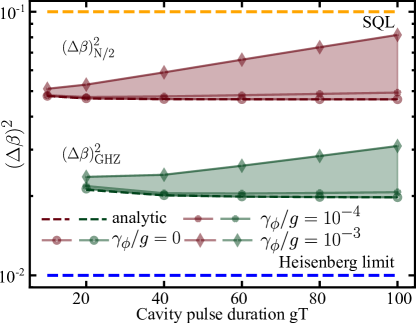
Figure S3: $(\Delta\beta)^{2}_{N/2}$ and $(\Delta\beta)^{2}_{\mathrm{GHZ}}$ obtained with our optimal state preparation protocol when local homogeneous dephasing of states $\ket{1}$ and $\ket{e}$ is added with rates $\gamma_{\phi}^{1}=\gamma_{\phi}^{e}=\gamma_{\phi}$, for $N=10$, $C=10^{2}$, $\gamma/\kappa=1.0$. The markers correspond to numerical results obtained with simulations performed with the effective model derived in Eq. (S22) in the collective Hilbert space. The dashed lines correspond to the values obtained with analytical solutions in Eqs. (S4)-(S5).

VI Spins under local homogeneous dephasing during signal collection

In this section we present the analytic expressions for the measured $(\Delta\beta)^{2}$ with ideal GHZ and $\ket{\mathcal{D}^{N}_{N/2}}$ states in the presence of local homogeneous dephasing of the spins as a function of time during signal acquisition in field sensing experiment, and further present the results of the measured $(\Delta\beta)^{2}$ with the optimal probe states obtained at finite cooperativities. The former expressions also provide approximate fitting functions to the latter.

VI.1 Analytic fit for GHZ-like states undergoing dephasing during signal collection

Analytical results of evolution of an ideal GHZ state acted upon by a field $\hat{H}_{\vec{z}}=J\hat{J}_{z}$ in the presence of local homogeneous dephasing on the spins are presented in Ref. [30]. We summarize the results here, and write the analytic expression for $(\Delta\beta)^{2}$ of ideal GHZ states (rotated by $\pi/2N$ along $z$ such that $\beta_{\mathrm{opt}}=0$).

In accordance with the definition of jump operator $\mathcal{A}_{j}=\frac{1}{2}\hat{\sigma}_{z}$ in the master equation dynamics(see main text), the local dephasing map on a single spin is defined as $\mathcal{A}_{t}(\hat{\sigma}_{x}\pm i\hat{\sigma}_{y})=e^{-i\frac{\gamma_{\phi}}{2}t}e^{\mp iJt}(\hat{\sigma}_{x}+i\hat{\sigma}_{y})$, and $\mathcal{A}_{t}(\hat{\sigma}_{z})=\hat{\sigma}_{z}$, $\mathcal{A}_{t}(\hat{\mathbb{I}})=\hat{\mathbb{I}}$. This map can be directly applied on the ideal GHZ state expanded as [30]

$$\rho_{GHZ}=\frac{1}{2^{N+1}}\left(\otimes_{j=1}^{N}(\hat{\mathbb{I}}+\hat{\sigma}_{z;j})+\otimes_{j=1}^{N}(\hat{\mathbb{I}}-\hat{\sigma}_{z;j})+\otimes_{j=1}^{N}(\hat{\sigma}_{x;j}+i\hat{\sigma}_{y;j})+\otimes_{j=1}^{N}(\hat{\sigma}_{x;j}-i\hat{\sigma}_{y;j})\right)$$

Now for the GHZ state rotated by $\pi/2N$ along $\hat{z}$ given by $e^{-i(\pi/2N)\hat{J}_{z}}\rho_{GHZ}e^{i(\pi/2N)\hat{J}_{z}}$, and under the dephasing map, for $\hat{M}=\mathcal{P}_{x}$ we obtain

$$\langle\hat{M}\rangle =e^{-N\frac{\gamma_{\phi}}{2}t}\cos{(NJt+\pi/2)},\quad(\Delta\hat{M})^{2}=1-e^{-N\gamma_{\phi}t}\cos^{2}{(NJt+\pi/2)},$$ (S23)

$$(\Delta Jt)^{2} =\frac{e^{N\gamma_{\phi}t}}{N^{2}}\frac{1-e^{-N\gamma_{\phi}t}\cos^{2}{(NJt+\pi/2)}}{|\sin{(NJt+\pi/2)}+(\gamma_{\phi}/2J)\cos{(NJt+\pi/2)}|^{2}}.$$ (S24)

For the obtained noisy GHZ-like optimal probe states, we fit $\langle\hat{M}\rangle$ with

$$\langle\hat{M}\rangle =\sum_{m=N/2}^{1}\alpha_{m}e^{-m\gamma_{\phi}t}\cos{(2m(Jt+\pi/(2N)))}+\alpha_{0},$$ (S25)

and expect a similar $\sim\exp{N\gamma_{\phi}t}$ scaling in $(\Delta Jt)^{2}$. For the case of $\gamma_{\phi}/J=0.01$ in Fig.2, we obtain non-zero fit parameters $\alpha_{N/2-1}=0.78$, $\alpha_{N/2-2}=0.16$, $\alpha_{0}=0.05$.

VI.2 Analytic fit for $\ket{\mathcal{D}^{N}_{N/2}}$-like states undergoing dephasing during signal collection

We can perform a similar calculation to evaluate the effect of dephasing during signal accumulation on the $\ket{\mathcal{D}^{N}_{N/2}}$ state by a field $\hat{H}_{\vec{y}}=J\hat{J}_{y}$. In this scenario, the map generated by the signal and that due to dephasing in the $\hat{z}$ basis do not commute. To simplify this calculation, we assume that the input state is a perfect $\ket{\mathcal{D}^{N}_{N/2}}$, which then undergoes dephasing at a rate $\gamma_{\phi}$ over a time $t$, followed by perfect rotation of the system by the unitary $U=e^{-iJt\hat{J}_{y}}$ without dephasing. This models a field profile where the field strength $J(\tau)$ is near zero until time $t$ where it turns on strongly so that the integrated action angle is $\beta=\int_{0}^{t}J(\tau)d\tau=Jt$. The variance of the estimation of $\beta$ given the measurement operator $\hat{M}=\hat{J}_{z}^{2}$ is given by [24]:

$$(\Delta\beta)^{2}=\frac{(\Delta\hat{J}_{x}^{2})^{2}f(\beta)+4\langle\hat{J}_{x}^{2}\rangle-3\langle\hat{J}_{y}^{2}\rangle-2\langle\hat{J}_{z}^{2}\rangle(1+\langle\hat{J}_{x}^{2}\rangle)+6\langle\hat{J}_{z}\hat{J}_{x}^{2}\hat{J}_{z}\rangle}{4(\langle\hat{J}_{x}^{2}\rangle-\langle\hat{J}_{z}^{2}\rangle)^{2}}$$ (S26)

where

$$f(\beta)=\frac{(\Delta\hat{J}_{z}^{2})^{2}}{\tan^{2}(\beta)(\Delta\hat{J}_{x}^{2})^{2}}+\tan^{2}(\beta).$$

Now we define the set of $n$ bit strings with Hamming weight $w$ as $\mathcal{B}^{n}_{w}=\{\vec{x}|\sum_{j}x_{j}=w\}$ and furthermore the distance between two binary strings as $d(\vec{x},\vec{y})=\sum_{j}|x_{j}-y_{j}|$. The Dicke state can be written

$$\ket{\mathcal{D}^{N}_{N/2}}=\sqrt{\frac{1}{\binom{N}{N/2}}}\sum_{\vec{x}\in\mathcal{B}^{n}_{w}}\ket{\vec{x}}\otimes\ket{\mathcal{D}^{N-n}_{N/2-w}}\sqrt{\binom{N-n}{N/2-w}}.$$

Let the output of dephasing map after time $t$ acting on a state $\rho$ be written $S_{t}(\rho)$. Notice that the expression for the variance in Eq. (S26) involves second and fourth moments of angular momentum operators. This fact together with the permutation invariance property of the Dicke states, and the local action of the dephasing map, implies that the we can focus on the action of the map on a decomposition of the input state into a partition of the state into a subsystem of the first two or four qubits and the rest. Specifically we have the following decomposition of the output state:

$$\begin{array}[]{lll}S_{t}\Big{(}\ket{\mathcal{D}^{N}_{N/2}}\bra{\mathcal{D}^{N}_{N/2}}\Big{)}&=&\frac{1}{\binom{N}{N/2}}\sum_{w}\sum_{\vec{x},\vec{y}\in\mathcal{B}^{j}_{w}}\ket{\vec{x}}\bra{\vec{y}}e^{-d(\vec{x},\vec{y})\gamma_{\phi}t}\otimes S_{t}\Big{(}\ket{\mathcal{D}^{N-j}_{N/2-w}}\bra{\mathcal{D}^{N-j}_{N/2-w}}\Big{)}{\binom{N-j}{N/2-w}}\\ &&+\Big{(}{\rm terms\ having\ }S_{t}\Big{(}\ket{\mathcal{D}^{N-j}_{N/2-w}}\bra{\mathcal{D}^{N-j}_{N/2-w^{\prime}}}\Big{)}{\rm with\ }w\neq w^{\prime}\Big{)}.\end{array}$$

where we can focus on this decomposition for $j=2,4$. The last terms which are off diagonal in the Dicke basis will not contribute to expectation values of weight $2$ or $4$ Pauli operators, when we take the trace, namely $\langle\hat{O}\rangle=\Tr[\hat{O}S_{t}\Big{(}\ket{\mathcal{D}^{N}_{N/2}}\bra{\mathcal{D}^{N}_{N/2}}\Big{)}]$. The input state is invariant under rotations about $\hat{z}$ as is the dephasing map so $\langle\hat{J}_{x}^{2}\rangle=\langle\hat{J}_{y}^{2}\rangle$. Also because there are an equal number of diagonal terms with even and odd Hamming weight we have $\langle\hat{J}_{z}^{2}\rangle=\langle\hat{J}_{z}^{4}\rangle=0$. Now we write

$$\hat{J}_{x}^{2}=\frac{1}{4}\sum_{j\neq k}X_{j}X_{k}+\frac{N}{4}{\bf 1},\quad\hat{J}_{x}^{4}=\frac{1}{16}\sum_{j\neq k,j^{\prime}\neq k^{\prime}}X_{j}X_{k}X_{j^{\prime}}X_{k^{\prime}}+\frac{N}{8}\sum_{j\neq k}X_{j}X_{k}+\frac{N^{2}}{16}{\bf 1}.,$$

For $\langle\hat{J}_{x}^{2}\rangle$ the two point expectation value

$$\langle X_{j}X_{k}\rangle=\frac{e^{-2\gamma_{\phi}t}N}{2(N-1)}$$

for $j\neq k$, of which there are $N(N-1)$ terms, and hence

$$\langle\hat{J}_{x}^{2}\rangle=\frac{1}{4}\Big{(}\frac{e^{-2\gamma_{\phi}t}N^{2}}{2}+N\Big{)}.$$

For $\langle\hat{J}_{x}^{4}\rangle$, the four point expectation value

$$\langle X_{j}X_{k}X_{\ell}X_{m}\rangle=\frac{e^{-4\gamma_{\phi}t}3N(N-2)}{8(N-1)(N-3)},$$

for $j\neq k\neq\ell\neq m$, of which there are $N(N-1)(N-2)(N-3)$ terms. The number of terms involving $\langle{\bf 1}\rangle$ are $3N^{2}-2N$. The remaining terms only involve two point expectation values $\langle X_{j}X_{k}\rangle$ with $j\neq k$ and there are $N^{4}-N(N-1)(N-2)(N-3)-(3N^{2}-2N)$ of them. Hence

$$\langle\hat{J}_{x}^{4}\rangle=\frac{1}{16}\Big{(}(3N^{2}-2N)+e^{-2\gamma_{\phi}t}(3N^{3}-4N^{2})+\frac{e^{-4\gamma_{\phi}t}3N^{2}(N-2)^{2}}{8}\Big{)}.$$

Finally, we find

$$\begin{array}[]{lll}\langle\hat{J}_{z}\hat{J}_{x}^{2}\hat{J}_{z}\rangle&=&\Tr[\hat{J}_{z}\hat{J}_{x}^{2}\hat{J}_{z}S_{t}\Big{(}\ket{\mathcal{D}^{N}_{N/2}}\bra{\mathcal{D}^{N}_{N/2}}\Big{)}]\\ &=&\Tr[\hat{J}_{x}^{2}\hat{J}_{z}S_{t}\Big{(}\ket{\mathcal{D}^{N}_{N/2}}\bra{\mathcal{D}^{N}_{N/2}}\Big{)}\hat{J}_{z}]\\ &=&\Tr[\hat{J}_{x}^{2}S_{t}\Big{(}\hat{J}_{z}\ket{\mathcal{D}^{N}_{N/2}}\bra{\mathcal{D}^{N}_{N/2}}\hat{J}_{z}\Big{)}]\\ &=&0\end{array}$$

using the fact that $\hat{J}_{z}$ commutes with the dephasing channel, and $\hat{J}_{z}\ket{\mathcal{D}^{N}_{N/2}}=0$. Hence we arrive at for $\beta=Jt$

$$(\Delta Jt)^{2}=\frac{16e^{2\gamma_{\phi}t}(2e^{2\gamma_{\phi}t}+N)+(16e^{4\gamma_{\phi}t}(N-1)+16e^{2\gamma_{\phi}t}N(N-2)+N(12-12N+N^{2}))\tan^{2}(Jt)}{8N(2e^{2\gamma_{\phi}t}+N)^{2}}.$$ (S27)

Notice as expected, at $t=0$ the variance $(\Delta\beta)^{2}=\frac{2}{N(N+2)}$.

In Fig.S4, we plot $(\Delta\beta)^{2}=(\Delta Jt)^{2}$ as a function of the signal acquisition time $Jt$ for ideal GHZ and $\ket{\mathcal{D}^{N}_{N/2}}$ probe states(panel (a)) with local homogeneous dephasing rates $\gamma_{\phi}/J=0,0.01,0.1,1.0$ for $N=10,40,60$ and compare their performance in field-sensing experiment against the performance of the optimal probe states(similar to Fig.2 but for longer signal collection times) prepared for $C=10^{4}$, $\gamma/\kappa=1.0$(panel (b)) and $C=10^{2}$, $\gamma/\kappa=1.0$(panel (c)). We observe a qualitatively similar behaviour of the optimal probe states prepared at finite cooperativities.

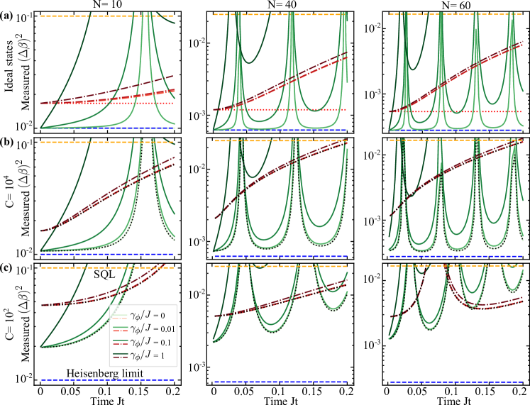
Figure S4: (a) $(\Delta\beta)^{2}=(\Delta Jt)^{2}$ as a function of dimensionless signal acquisition time $Jt$ for ideal GHZ states and ideal $\ket{\mathcal{D}^{N}_{N/2}}$ states evolving under a field coupled with strength $J$ with local homogeneous dephasing acting on spins obtained in Eqs. (S24) and  (S27) respectively, for dephasing rates $\gamma_{\phi}/J=0,0.01,0.1,1.0$ and $N=10,40,60$. The dotted red lines correspond to $(\Delta\beta)^{2}=2/(N(N+2)$. (b) Measured $(\Delta\beta)^{2}$ as a function of dimensionless signal acquisition time $Jt$ by numerically evolving the optimal probe states prepared at cooperativity $C=10^{4}$, $\gamma/\kappa=1.0$ under a field coupled with spins with coupling strength $J$, with local dephasing on spins with rates $\gamma_{\phi}$ (for similar values as in panel (a)). Dotted black curves are the optimal $(\Delta\beta)^{2}$ obtained with analytic solution of $\mathcal{E}_{\mathrm{gpg}}$ for $\gamma_{\phi}/J=0$. (c) Similar to panel (b) for optimal states prepared at cooperativity $C=10^{2}$, $\gamma/\kappa=1.0$. The cooperativity $C$ values corresponding to an entire panel (row) and $N$ values corresponding to an entire column are indicated to the left and the top sides respectively. Throughout, green solid lines (darker shades for larger $\gamma_{\phi}$) correspond to GHZ-like states while red dash-dot lines correspond to $\ket{\mathcal{D}^{N}_{N/2}}$ states.

VII Local homogeneous spontaneous emission treated as a collective process

In this section, we treat the local homogeneous spontaneous emission rate $\gamma$ of state $|e\rangle$ in the master equation approach with jump operator $\mathcal{A}_{\gamma}^{(j)}=\ket{1_{j}}\bra{e_{j}}$. The transformed jump operator $\tilde{\mathcal{A}_{\gamma}^{(j)}}=\hat{U}\mathcal{A}_{\gamma}^{(j)}\hat{U}^{\dagger}$(similar to qubit basis transformation performed in Eqs. (S18)-(S19)) is obtained as

$$\tilde{\mathcal{A}^{(j)}_{\gamma}} = \mathcal{A}^{(j)}_{\gamma}\frac{1}{2}\left(1+\sqrt{1-4|\zeta|^{2}/g^{2}}\right)$$ (S28)

$$-(\mathcal{A}^{(j)}_{\gamma_{\phi}^{e}}-\mathcal{A}^{(j)}_{\gamma_{\phi}^{1}})e^{i\psi}(|\zeta|/g)$$

$$-(\mathcal{A}^{(j)}_{\gamma})^{\dagger}\frac{e^{i2\psi}}{2}\left(1-\sqrt{1-4|\zeta|^{2}/g^{2}}\right).$$

We obtain a similar effective Lindbladian $\mathcal{L}_{\mathrm{eff}}$ in the same form as in Eqs. (S20), with

$$\gamma_{\phi}^{\prime}=\gamma|\zeta|^{2}/g^{2},\hskip 10.00002pt\mathcal{A}_{\gamma_{\phi}^{\prime}}=\frac{1}{2}\sigma_{z}^{(j)},$$ (S29)

$$\gamma^{\prime}=\gamma\frac{(1-\sqrt{(1-4|\zeta|^{2}/g^{2})})^{2}}{4}.$$ (S30)

The effective model is reduced to

$$\hat{H}_{\mathrm{eff}} = \delta\hat{a}^{\dagger}\hat{a}+\left(-i\frac{\gamma^{\prime}}{2}+\zeta\hat{a}^{\dagger}+\zeta^{*}\hat{a}\right)\hat{n}_{1},$$ (S31)

$$\mathcal{L}[\rho_{\mathrm{eff}}] = \kappa\mathcal{L}_{\kappa}[\rho_{\mathrm{eff}}]+\gamma^{\prime}_{\phi}\sum_{j=1}^{N}\mathcal{L}_{\gamma^{\prime}_{\phi}}^{(j)}[\rho_{\mathrm{eff}}].$$ (S32)

In Fig. S5, $(\Delta\beta)^{2}_{N/2}$ and $(\Delta\beta)^{2}_{\mathrm{GHZ}}$ is plotted by simulating the master equation dynamics with the model described above (solid lines). It is compared against the values obtained when $\gamma$ is treated as a non-hermitian contribution (dashed lines, model described in the main text, see Eq. (1)). We see that the solid lines always lie very close or below the dashed lines, hence implying an upper bound on the variance corresponding to the $(\Delta\beta)^{2}$ values obtained in the main text by treating $\gamma$ as a non-hermitian contribution.

Figure S5: $(\Delta\beta)^{2}_{N/2}$ and $(\Delta\beta)^{2}_{\mathrm{GHZ}}$ obtained with our optimal state preparation protocol with the spontaneous emission from the $\ket{e}$ state is treated as a non-hermitian contribution (dashed lines, star markers) compared with the values obtained when decay is treated as a Lindbladian jump operator in the master equation formalism(solid lines, circle markers).

References

Jozsa and Linden [2003]R. Jozsa and N. Linden, Proceedings of the Royal Society of London. Series A: Mathematical, Physical and Engineering Sciences 459, 2011 (2003).
Huang et al. [2024]J. Huang, M. Zhuang, and C. Lee, arXiv preprint arXiv:2402.03572 (2024).
Leroux et al. [2010]I. D. Leroux, M. H. Schleier-Smith, and V. Vuletić, Physical Review Letters 104, 073602 (2010).
Schleier-Smith et al. [2010]M. H. Schleier-Smith, I. D. Leroux, and V. Vuletić, Physical review letters 104, 073604 (2010).
Cox et al. [2016]K. C. Cox, G. P. Greve, J. M. Weiner, and J. K. Thompson, Physical review letters 116, 093602 (2016).
Bohnet et al. [2016]J. G. Bohnet, B. C. Sawyer, J. W. Britton, M. L. Wall, A. M. Rey, M. Foss-Feig, and J. J. Bollinger, Science 352, 1297 (2016).
Pedrozo-Peñafiel et al. [2020]E. Pedrozo-Peñafiel, S. Colombo, C. Shu, A. F. Adiyatullin, Z. Li, E. Mendez, B. Braverman, A. Kawasaki, D. Akamatsu, Y. Xiao, et al., Nature 588, 414 (2020).
Jandura et al. [2023]S. Jandura, V. Srivastava, G. Brennen, and G. Pupillo, arXiv:2303.13127 (2023).
[13]The cavity drive pulse in the original frame is obtained by inverting the pulse in Eq. (1) with a finite value of which is set by a choice of . Here, we make a choice of .
[15]See Supplemental Material where the decay from with rate is also included as a local-homogeneous collective process in the Lindblad master equation defined in a collective Hilbert space(see Ref. [27]).
Gutman et al. [2024]N. Gutman, A. Gorlach, O. Tziperman, R. Ruimy, and I. Kaminer, Physical Review Letters 132, 153601 (2024).
Bond et al. [2023]L. J. Bond, M. J. Davis, J. Minář, R. Gerritsma, G. K. Brennen, and A. Safavi-Naini, arXiv preprint arXiv:2312.05060 (2023).
Braunstein and Caves [1994]S. L. Braunstein and C. M. Caves, Physical Review Letters 72, 3439 (1994).
[19]Without loss of generality, we set by adding a step in the protocol corresponding to global qubit rotation by the found along the field-axis (known).
[20]G. Scheithauer, Jorge nocedal and stephen j. wright: Numerical optimization, springer series in operations research, 1999, isbn 0-387-98793-2.
Leibfried et al. [2004]D. Leibfried, M. D. Barrett, T. Schaetz, J. Britton, J. Chiaverini, W. M. Itano, J. D. Jost, C. Langer, and D. J. Wineland, Science 304, 1476 (2004).
Lücke et al. [2011]B. Lücke, M. Scherer, J. Kruse, L. Pezzé, F. Deuretzbacher, P. Hyllus, O. Topic, J. Peise, W. Ertmer, J. Arlt, et al., Science 334, 773 (2011).
Apellaniz et al. [2015]I. Apellaniz, B. Lücke, J. Peise, C. Klempt, and G. Tóth, New Journal of Physics 17, 083027 (2015).
Kuhr et al. [2005]S. Kuhr, W. Alt, D. Schrader, I. Dotsenko, Y. Miroshnychenko, A. Rauschenbeutel, and D. Meschede, Physical Review A 72, 023406 (2005).
Chase and Geremia [2008]B. A. Chase and J. Geremia, Physical Review A 78, 052101 (2008).
Shammah et al. [2018]N. Shammah, S. Ahmed, N. Lambert, S. De Liberato, and F. Nori, Physical Review A 98, 063815 (2018).
[29]See Supplemental Material for analytic fits and results for different and values, and for longer collection times.
Shaji and Caves [2007]A. Shaji and C. M. Caves, Physical Review A—Atomic, Molecular, and Optical Physics 76, 032111 (2007).
Barontini et al. [2015]G. Barontini, L. Hohmann, F. Haas, J. Estève, and J. Reichel, Science 349, 1317 (2015).
Manetsch et al. [2024]H. J. Manetsch, G. Nomura, E. Bataille, K. H. Leung, X. Lv, and M. Endres, arXiv preprint arXiv:2403.12021 (2024).
Li et al. [2012]J. Li, M. A. Sillanpää, G. Paraoanu, and P. J. Hakonen, in Journal of Physics: Conference Series, Vol. 400 (IOP Publishing, 2012) p. 042039.