The number of minima in random landscapes generated by constrained random walk and Lévy flights: universal properties
Abstract
We provide a uniform framework to compute the exact distribution of the number of minima/maxima in three different random walk landscape models in one dimension. The landscape is generated by the trajectory of a discrete-time continuous space random walk with arbitrary symmetric and continuous jump distribution at each step. In model I, we consider a “free” random walk of steps. In model II, we consider a “meander landscape” where the random walk, starting at the origin, stays non-negative up to steps. In model III, we study a “first-passage landscape” which is generated by the trajectory of a random walk that starts at the origin and stops when it crosses the origin for the first time. We demonstrate that while the exact distribution of the number of minima is different in the three models, for each model it is universal for all , in the sense that it does not depend on the jump distribution as long as it is symmetric and continuous. In the last two cases we show that this universality follows from a non trivial mapping to the Sparre Andersen theorem known for the first-passage probability of discrete-time random walks with symmetric and continuous jump distribution. Our analytical results are in excellent agreement with our numerical simulations.
I Introduction
A typical realisation of a random landscape in dimension consists of local minima, local maxima and saddle points. How many such stationary points are there in a given realisation of the landscape? How do these numbers fluctuate from sample to sample? These are fundamentally important questions in a wide variety of fields including physics, chemistry, mathematics and computer science Adler ; Azais ; Freund (1995); Halperin and Lax (1966); Broderix et al. (2000); Longuet-Higgins (1960); halperin_82 ; Ros_Fyo_23 . For example, in liquids or glassy systems, the statistics of such stationary points provide information on the complexity (entropy) of metastable states Bray and Moore (1980); Annibale et al. (2003); Aspelmeier et al. (2004); Satya_Martin ; Hivert ; Sollich . The same question also appears in string theory Aazami and Easther (2006); Susskind (2003), random matrix theory and also in the characterisation of the fitness landscapes in evolutionary biology Barton (2005); Krug_review ; Krug_fitness1 ; Krug_fitness2 . Another application appears in optics, where one needs to estimate the number of specular points on a random reflecting surface. Similarly, the intensity of the electric field of speckle laser patterns requires the knowledge of the number of stationary points of a Gaussian random field Longuet-Higgins (1960); halperin_82 . This estimation problem also recently appeared in computer science problems dealing with big data where one wants to perform non-convex optimisation of large dimensional data Ganguli_14 . Most of these studies concentrated on calculating just the mean number of stationary points of a random landscape, for instance by using the Kac-Rice formalism Rice . However, computing the full distribution of the number of such stationary points has largely remained open, except for uncorrelated landscape. In this latter case, the full distribution can be shown to follow Gaussian statistics via the Central Limit Theorem Satya_Martin ; Hivert ; Sollich .
Thus computing the full distribution of the number of minima, maxima or saddles in a correlated landscape is a difficult and important problem. In a recent paper KMS24 , we have computed the full distribution of the number of minima/maxima in a one-dimensional correlated landscape generated by the trail of a discrete-time random walk. More precisely, the random landscape of size in this model is just the spatial trajectory of a discrete-time random walk of steps with arbitrary symmetric jump distribution at each step. We found that the distribution of the number of minima , given the size of the landscape, is completely universal for any , i.e., independent of the jump distribution as long as it is symmetric. This was proved by solving an exact recursion relation. Moreover, in this work, we found, rather strikingly, that the distribution of the number of minima is also universal for a different random walk landscape, which we called the “first-passage landscape”. This first-passage landscape is generated by the trajectory of a discrete-time random walk till its first crossing of the origin. The reasons behind the universality in these two models were found to be quite different. In the first-passage landscape model, the universality emerged due to a deep connection KMS24 between the combinatorial problem of counting the number of local minima of such a landscape and the Sparre Andersen theorem of Markov jump processes known in probability theory SA1954 .
The purpose of this paper is to provide a unified framework that can be used to derive the universal results for the statistics of the number of minima/maxima in both landscape models, namely the free walk and the first-passage walk. Furthermore, we show that this unified framework can be extended to derive universal results for yet another constrained random walk landscape, namely the “meander landscape”. This meander landscape is generated by the trajectory of a random walker of steps that starts at zero and remains nonnegative up to steps. Our unified framework is based on an exact mapping between the statistics of the number of minima of such constrained random walk landscapes and the first-passage property of an effective auxiliary random walk. This allows us to derive the full distribution of the number of minima for all and also proving their universalities for the three classes of random walk landscapes. Our analytical predictions are verified by numerical simulations, finding excellent agreement.
The rest of the paper is organized as follows. In Section II, we define the model, the observables of interest and also provide a short summary of the main results. In Section III, we establish an exact mapping between the statistics of the number of minima and the first-passage property of an auxiliary random walk problem. In Section IV we use this mapping to compute the full distribution of the number of minima for a free random walk of steps. Section V deals with the exact distribution of a landscape generated by a random walk meander, using this mapping. Finally, in Section VI we show how this mapping can be used to compute exactly the distribution of the number of minima in a first-passage landscape. Section VI provides a summary and conclusion.
II The model, the observables and the summary of the main results
We consider a discrete-time, continuous-space random walker/Lévy flight on a line whose position at step evolves via the Markov jump process
| (1) |
where ’s are independent and identically distributed (IID) jump lengths, each drawn from a symmetric and continuous probability distribution function (PDF) , which is normalized to unity, . Because of the symmetry, the mean jump length vanishes identically, . If the variance is finite, the walk converges, for large , to the Brownian motion via central limit theorem. In constrast, for Lévy flights where with the Lévy index , the variance of the jump length is infinite due to the presence of very long jumps.
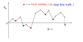
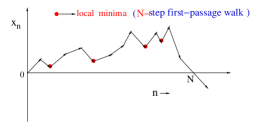
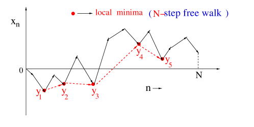
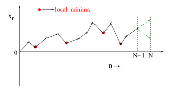
In this paper, we consider such a random walk/Lévy flight of steps, starting at the origin, but subjected to different spatial constraints. We study three different constrained walks: (I) an -step free random walk (II) an -step meander random walk where the walker is constrained to stay non-negative up to -steps and (III) an -step random walk that stays positive up to steps and crosses the origin to the negative side exactly at step –we refer to it as an -step first-passage walk (see Fig. (1)). In each model, we count the number of local minima in a trajectory of steps. Clearly, is a random variable that fluctuates from one trajectory to another in any given model. We are interested in computing the the distribution of the number of local minima , for fixed , in all the three models , and . More precisely, we define the following three probabilities:
-
(I)
Probobility of having local minima in an -step free random walk evolving via Eq. (1), starting from the origin.
-
(II)
Joint probability that the random walk, starting at the origin, stays positive up to step and that the trajectory has local minima. The subscript ‘me’ denotes a meander.
-
(III)
Joint probability that the random walk, starting at the origin, stays positive up to step and crosses the origin to the negative side at step and that the walk has local minima. The subscript ‘fp’ stands for a first-passage walk.
Our main results can be summarized as follows. We show that all three probabilities listed above are completely universal for all and all , i.e., independent of the jump PDF , as long as it is continuous and symmetric. In Model (I), it does not even need to be continuous. The exact and explicit expressions for the three probablities are given below.
-
•
Model I. In this case we show that
(2) -
•
Model II. For the -step meander walk, we prove that
(3) -
•
Model III. For the -step first-passage walk, we prove that for all
(4) For , we have .
We show that all the three exact results in Eqs. (2), (3) and (4) can be derived from the same basic ingredient, namely, by exploiting an exact mapping to an auxiliary random walk that transits from one local minima to the next. We will also see that while the universality in model I emerges from local properties of the noise variables (two successive independent jumps in the walk having respectively negative and positive directions create a local minimum), the mechanism responsible for the universality in models II and III is much more nontrivial since the actual space (and not just the signatures of local jumps) is involved. We will see that in these last two models, the universality emerges as a consequence of the Sparre Andersen theorem applied to the auxiliary random walk connecting the local minima.
The result for for an -step free random walk in Eq. (2) was derived recently in Ref. KMS24 by using an alternative method. In addition, the result for the sum was also derived in Ref. KMS24 . However, the results for in Eq. (3), as well as that of in Eq. (4), valid for arbitrary (and not just the sum over ), are new. Numerical simulations are in excellent agreement with our analytical predictions in Eqs. (2)-(4).
III Basic ingredients: an exact mapping to an auxilary random walk
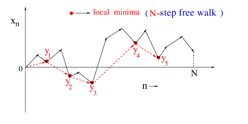
In this section, we will see that the statistics of minima in a random walk landscape generated via Eq. (1), in the presence or the absence of constraints, can be most conveniently computed by exploiting an exact mapping to an auxiliary random walk problem connecting only the local minima–we will refer to it as the minima random walk (MRW). To see how this mapping works, we consider any arbitrary -step trajectory of the random walk generated via Eq. (1), as shown in Fig. (2). We locate the local minima and denote their positions by where is the number of local minima in the trajectory. We join these local minima by dashed lines and also connect the origin to the first minima at location (as in Fig. (2)). This set then forms the trajectory of an auxiliary random walk (we call it MRW), where the MRW jumps from to at the -th step. Note that the number of steps of the original walk between two successive positions of MRW (say between and ) is not fixed and varies from trajectory to trajectory. Our first goal is to compute the transition probability density of the MRW to arrive at , starting from , in steps of the original random walk.
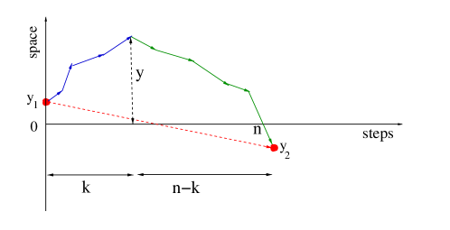
To compute the transition probability density , let us consider the -step segment of the original walk between two successive local minima with heights and respectively, as shown in Fig. (3). The first observation is that since and are successive local minima by definition, there can not be another local minumum inside the segment and the number of steps in the segment must be atleast , i.e., . Also, there must be one and only one local maximum in the interior of this segment (see Fig. (3)). Clearly, the segment must start from with an upward jump and continue with upward jumps till it reaches the local maximum, say at height and then come down to only via negative jumps. The local maximum then divides the segment of steps into the left part of upward jumps and a right part of downward jumps. We refer to the left part as a monotonically upward segment (MUS) and the right part as the monotonically downward segment (MDS). Let and denote the number of steps belonging respectively to the MUS and MDS in a particular configuration (and eventually we will sum over all allowed values of ). Clearly . We also note that , since is the height of the maximum between and .
Let us first focus on the segment MUS consisting of upward jumps only. Let denote the probability density of reaching , starting from , after successive positive jumps of the original walk in Eq. (1). Then satisfies
| (5) |
starting from . To exploit the convolution structure in Eq. (5), it is useful to define the Laplace transform
| (6) |
Consequently, taking Laplace transform of Eq. (5) and using the convolution property, we get
| (7) |
where
| (8) |
Note that since we assume that the jump distribution is symmetric and is normalized to unity on the whole line, we have from Eq. (8)
| (9) |
Consequently, from Eq. (7), we have
| (10) |
It is also useful to define the generating function
| (11) |
Integrating over , using (10) gives
| (12) |
Finally, we note that since the jump distribution of the original walk is symmetric, it follows that for the MDS, i.e., the monotonically downward segment on the right of the maximum, will have the same statistics as the MUS on the left of the maximum. In addition, the two segments MUS and MDS are statistically independent due to the Markov property of the walk.
Armed with the basic ingredients developed above, we can now write down the transition probability density of the auxiliary random walk MRW connecting successive local minima. Using the independence of MUS and MDS and the fact that they have the same statistics, we can write
| (13) |
where denotes the height of the maximum between and (see Fig. (3)), and is computed above. Taking generating function with respect to , and using (11), we get
| (14) |
Note that the sum over starts from since the number of steps of the origin walk between two successive local minima must be at least . Making further a shift in the integral in (14), we get
| (15) |
This shows that is only a function of the difference , and hence we can write
| (16) |
where is a symmetric function of . In addition, this function is non-negative for all and its normalization can be explicitly worked out as follows. Integrating over and using the symmetry in (16) gives
| (17) |
Finally, using (12) gives
| (18) |
Note that this generating function can easily be inverted to obtain
| (19) |
This result can be understood as follows (see Fig. 3): the factor corresponds to the probability for the random walk to perform positive steps followed by negative steps, while the factor takes into account the different positions of the maximum, with . It is further useful to define the function
| (20) |
such that is a symmetric non-negative function of , parametrized by , and is normalized to unity
| (21) |
Thus, to summarize, the generating function of the transition probability density can be exressed as
| (22) |
where can be interpreted as a continuous and symmetric PDF normalized to unity. Eq. (22) is the main result of this section. We will see in later sections that we can then use the result in (22) as the basic building block that will enable us to compute exactly the statistics of several observables of the MRW. Note that depends, of course, on the original jump PDF , since depends on as in Eq. (15) which, in turn, depends explicitly on and via Eq. (11). However, we will see below that we would not need this explicit dependence of on to establish our universal results on the statistics of the number of local minima that do not depend on . Just the fact that can be interpreted as a symmetric, continuous, normalized to unity PDF will be sufficient for us.
IV Number of local minima in model I : -step free walk
Using the basic building blocks developed in the previous section, here we first apply them to compute the distribution of the number of local minima in an -step free random walk. In order to use the results of the previous section, it is useful to first consider an extended joint probability of having local minima and their positions for an -step original free random walk. Once we have this extended joint probability, we can compute the marginal by integrating over the ’s, i.e.,
| (23) |
To compute the joint probability , it is further convenient to break it into two pieces
| (24) |
where denote the probability of the trajectory that starts with a positive or negative jump respectively. This amounts to splitting
| (25) |
where
| (26) |
We will see that these two probabilities will be diferent.
To proceed, we start by computing the joint probability . We first consider the event . The case is a bit special and will be treated later. It is easier to compute its generating function
| (27) |
that effectively attaches a weight to each jump of the original random walk. We start with in (27) since to have a number of local minima , the total number of steps must be at least . A typical trajectory contributing to this probability is shown in Fig. (2). Using the mapping to MRW, this trajectory consists of independent blocks connecting successive local minima and the origin and then a ‘dangling’ segment at the end, after the -th minimum (see Fig. (2)). This dangling segment can be of two types: (a) either all jumps in this segement are upwards, i.e., an MUS or (b) this segment may consist of a left segment with only upward jumps followed by a right segment of only downward jumps. So, we need to compute separately the weights of this dangling segment, after integrating out the final position at the end of the dangling segment. In case (a), where only upward jumps occur, the dangling segment contributes a weight (this follows from Eq. (12)). In case (b), since there is an MUS followed by a statistically indepedent MDS, the corresponding weight factor is just . Hence, the total weight of the dangling segment to the generating function is given by
| (28) |
Using this result and the independence of blocks of the MRW, we can then write, for ,
| (29) | |||||
where we used Eq. (28) for the dangling sector and Eq. (22) for each of the blocks of the MRW preceding the dangling sector. We recall that is normalized to unity as in Eq. (21). Now, integrating over using (21) we get
| (30) |
We now consider the case which is a bit special. In this case, only the dangling segment contributes, and we get, using Eq. (28)
| (31) |
Now, using this result and the fact that (since in one step the probability that the walk goes up is exactly ), we get
| (32) |
Hence summarzing, we get
Let us remark that this result in Eq. (IV) coincides with Eq. (S18) of Ref. KMS24 where it was derived by a completely different method.
We now turn to computing the joint probability , where the first jump from the origin is negative. A typical trajectory contributing to is shown in Fig. (4). As before, we first consider the event and the case will be treated separately. As in the previous case, it is easier to compute the generating function
| (33) |
where, by definition, . From Fig. (4) it is clear that the trajectory can be broken into blocks connecting the successive local minima and the two end segments. The segment at the end, i.e., after the -th minimum, is just the dangling segment whose weight was already computed in Eq. (28). The segement at the begining, connecting the origin to the first local minimum at consists of only downward jumps, starting at the origin and ending at , with . By using the up-down symmetry of the jump distribution, the weight of this segment is exactly identical to where is defined in Eq. (11). Taking the product of the weights of these three parts and using their independence, we can then write
| (34) | |||||
where the dangling sector contributes the factor . We next integrate over and over for all , use Eq. (12) and (21), to get
| (35) |
Let us now consider the case , with the first jump negative. In this case, the only configuration that contributes consists of only downward jumps. Hence we have, trivially, using Eq. (12)
| (36) |
Using we then get
| (37) |
Hence summarzing, we get
This result coincides with Eq. (S19) of Ref. KMS24 where it was derived by a different method.
Taking the generating function of the sum in Eq. (25)
| (38) |
and adding Eqs. (IV) and (IV) we get
Expanding the right hand side (rhs) of Eq. (IV) in powers of using the identity
| (39) |
and matching powers of on both sides gives
| (40) |
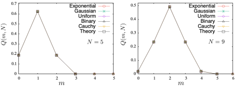
thus completing the derivation of the result announced in Eq. (2). Clearly is completely universal, i.e., independent of the jump distribution , as long as is symmetric. In Fig. (5) we compare our theoretical prediction (40) with direct numerical simulations, finding excellent agreement. As mentioned earlier, this result in Eq. (40) was already derived in Ref. KMS24 by a different method. But here we provide a derivation based on a more general method that can be easily extended to compute the distribution of the number of local minima for other constrained random walks, as shown in the next two sections. We also note that this result in (40) was derived in Marckert for lattice random walks (i.e., with jumps), but here we have shown that it is more general and holds for random walks with arbitrary symmetric jump distribution.
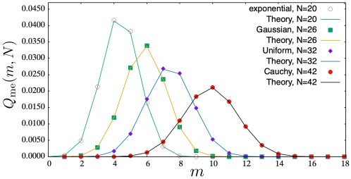
V Number of local minima in model II : -step meander walk
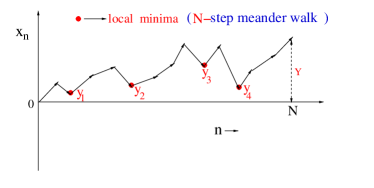
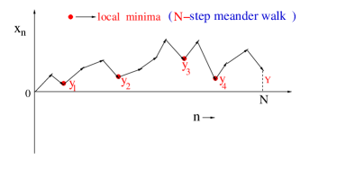
In this section we compute denoting the probability that the random walk in Eq. (1) remains non-negative up to step and that it has local minima. As in the previous section, it is convenient to first compute the extended joint distribution of the positions of the local minima and their number and then integrate out the positions of the local minima. But for the meander, one needs to be careful about the ‘dangling’ segment, i.e., the portion of the walk beyond the -th minimum. The last jump of this dangling sector can be either positive (as in the left panel of Fig. (6)) or negative (as in the right panel of Fig. (6)). One also needs to keep track of the position of the last point of the walk (see Fig. (6)). We first split the probability of having minima into two parts depending on whether the last jump is positive or negative
| (41) |
Similarly, we split the extended joint probability accordingly
| (42) |
such that
| (43) | |||||
| (44) |
We remark that the variables are integrated in the semi-infinite domain since we want the walk to remain non-negative. We note that in Eq. (43), the limit of integration over is over . This s because, the dangling segment in this case is monotonically increasing and hence we must have . In contrast, in Eq. (44), can take any value in , since the dangling segment now consists of an MUS followed by an MDS.
We start by writing down the expression for , or rather for its generating function
| (45) |
From the left panel of Fig. (6), it is clear that the weight of the dangling segment is an MUS and hence is given by , where is defined in Eq. (11). Then, we have
| (46) |
Consequently, by taking the generating function of Eq. (43), and using the result from Eq. (12), we get
| (47) |
where we have defined
| (48) |
Note, however, that since can be interpreted as the symmetric, continuous and normalized PDF of the jumps of the MRW (parametrized by ), the quantity is just the survival probablity of the MRW, starting at the origin, up to steps. By the celebrated Sparre Andersen theorem SA1954 , this survival probability is completely universal, i.e., independent of and is given by the formula
| (49) |
We now turn to the right panel of Fig. (6) where the last jump is negative. We define the generating function
| (50) |
From the right panel of Fig. (6), it is clear that the dangling segment now consists of a monotonically increasing stretch followed by a monotonically decreasing stretch ending at . Thus the dangling sector is very similar to any other interior block connecting and and hence carries a weight . Consequently, we get
| (51) |
Taking the generating function of Eq. (44) and integrating over the variables in the semi-infinite domain we get
| (52) |
Adding Eqs. (47) and (52) gives
| (53) |
where given in (49) is universal for all . This proves that is also universal, i.e., does not depend on the original jump distribution , as long as it is symmetric and continuous. Expanding the rhs of Eq. (53) in powers of using the identity (39) and reading off the coefficient of , it is easy to see that for
| (54) |
while for . Using from Eq. (49) and simplifying, we then get our final result announce in Eq. (3), namely
| (55) |
This analytical result is compared to numerical simulation in Fig. (7), finding excellent agreement.
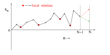
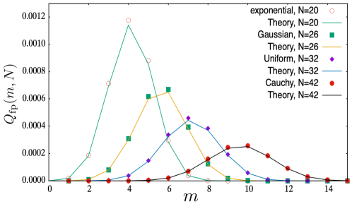
VI Number of local minima in model III: first-passage walk
In this section we compute denoting the joint distribution that the random walk in Eq. (1) crosses the origin from the positive side for the first time at step and that it has minima till this first crossing. For a typical trajectory contributing to , see the right panel in Fig. (1). We will see below that this probability can be related to the probabilities for an -step meander walk defined in Eqs. (43) and (44) and whose generating functions are explicitly computed respectively in Eqs. (47) and (52).
In order to make this connection to meander random walk discussed in the previous section we proceed as follows. Consider a typical trajectory contributing to in the right panel of Fig. (1). This walk clearly has to stay positive up to step and then has to cross to the negative side at step . We recall that denotes the probability that the walk stays positive up to step (with the last jump positive or negative) and that it has minima. Also, . Now, it is instructive to see what happens at the -th step. There are two possibilities. A walk that stays positive up to the -th. step, may either stay positive after the -th jump, or may cross the origin exactly at the -th step. Adding these two possibilities, we note that then denotes the probability that a walk stays positive up to steps and has local minima. Now, a local minimum may or may not form exactly at the -th step. If the former happens, the meander walk must have minima till the -th step and a new minima occurs exactly at the -th step, contributing to the event of minima up to steps. In the latter case, the meander walk must have already minima up to steps and no new minimum forms after the -th jump. In order to keep track of this last-step event, we need to consider a meander walk up to steps with the -th jump either positive or negative (as shown respectively in the left and the right panel of Fig. (8)). If the -th step is positive, then no matter what the sign of the -th jump is, there is no possibility of forming a new local minimum by the -th jump (see the left panel of Fig. (8)). In contrast, if the -th jump is negative, then there are two possibilities: (i) if the -th jump is positive (which occurs with probability ), then a new minimum forms exactly after the -th jump and (ii) if the -th jump is negative (which also occurs with probability ), no new minimum is generated at the -th step. Considering these possibilities, it is then easy to write down the following exact recursion relation
| (56) |
where the first term on the rhs refers to the event when the -th jump of the meander is positive (in that case it has to have minima till steps since no new minimum is generated at the -th step), while the last two terms counts the probability of events (i) and (ii) described above. Using Eq. (56) and the definition , we can then express in terms of the known quantities as
| (57) |
This recursion relation actually holds for and , with the convention that and . For the special case , one can similarly write down the recursion relation
| (58) |
Thus, we can actually include the term in the general recursion relation (57) valid for , provided we interpret . From now on we use this convention and hence Eq. (57) is valid for all and .
To proceed, we define the generating function
| (59) |
Taking generating function of Eq. (57) and using the convention and , we get
| (60) |
where . Using the explicit results for derived respectively in Eqs. (47) and (52), we get, after a few simplifying steps,
| (61) |
where is given in Eq. (49). Using this explicit result for , Eq. (61) reduces to
| (62) |
Let us remark that by setting in (62), and using , we obtain
| (63) |
thus recovering the result that was derived in Ref. KMS24 by a slightly different method. We next use the identity (39) to expand the rhs in powers of and then match the powers of on both sides of Eq. (62). This then gives the desired result (4), namely, for all
| (64) |
and for , we get . These analytical predictions are compared to numerical simulations in Fig. (9), finding excellent agreement.
VII Summary and Conclusion
In this paper we have provided a unified framework to compute the exact distribution of the number of minima/maxima in three one-dimensional random walk landscapes. The first landscape corresponds to the trajectory of a free discrete-time random walk of steps with arbitrary symmetric jump distribution at each step. The second “meander landscape” model corresponds to the trajectory a constrained random walk that starts at the origin and remains non-negative up to step . In the third “first-passage landscape ” we consider a random walk trajectory that starts at the origin and stops when it crosses the origin for the first time. Unlike in the first two models, here the number of steps of the landscape is a random variable that fluctuates from sample to sample. Our main result is to show that while the exact distribution of the number of minima is different in the three models, for each model it is universal for all , in the sense that it does not depend on the jump distribution as long as it is symmetric and continuous. In the last two cases we show that this universality follows from a deep connection to the Sparre Andersen theorem known for the first-passage probability of discrete-time random walks with symmetric and continuous jump distribution. Our analytical results are in excellent agreement with our numerical simulations.
There are many directions in which this work can be extended. For example, in Ref. KMS24 , we showed that, for a free random walk landscape the joint distribution of the number of minima and maxima up to steps is also universal and can be computed explicitly. It would be interesting to compute this joint distribution for the other two constrained random walk landscape models discussed in this paper and see whether there are also universal. The unified framework developed here via the mapping to the auxiliary random walk may be possible to use to compute the distribution of the number of minima or maxima (sometimes called “peaks”) for other constrained random walks, such as the random walk bridge or random walk excursion, as it was done for lattice random walks Marckert . Finally, it would be interesting to extend these studies of the statistics of the number of local minima, maxima and saddles to correlated landscapes in higher dimensions.
Acknowledgements.
The authors would like to thank the Isaac Newton Institute for Mathematical Sciences, Cambridge, for support and hospitality during the programmes New statistical physics in living matter: non equilibrium states under adaptive control and Stochastic systems for anomalous diffusion. where work on this paper was undertaken. This work was supported by by EPSRC Grant Number EP/R014604/1 and EPSRC grant no EP/K032208/1. SNM and GS acknowledge support from ANR Grant No. ANR-23-CE30-0020-01 EDIPS. SNM acknowledges the support from the Science and Engineering Research Board (SERB, Government of India), under the VAJRA faculty scheme (No. VJR/2017/000110). AK would like to acknowledge the support of DST, Government of India Grant under Project No. CRG/2021/002455 and the MATRICS Grant No. MTR/2021/000350 from the SERB, DST, Government of India. AK acknowledges the Department of Atomic Energy, Government of India, for their support under Project No. RTI4001.References
- (1) R. J. Adler, J. E. Taylor, Random Fields and Geometry (Berlin: Springer), (2009)
- (2) J.-M. Azaïs, M. Wschebor, Level Sets and Extrema of Random Processes and Fields, (New York: Wiley), (2009)
- Freund (1995) I. Freund, Phys. Rev. E, 52, 2348 (1995).
- Halperin and Lax (1966) B. Halperin and M. Lax, Phys. Rev., 148, 722 (1966).
- Broderix et al. (2000) K. Broderix, K. K. Bhattacharya, A. Cavagna, A. Zippelius, and I. Giardina, Phys. Rev. Lett., 85, 5360 (2000).
- Longuet-Higgins (1960) M. Longuet-Higgins, JOSA, 50, 845 (1960).
- (7) A. Weinrib, B. I. Halperin, Phys. Rev. B 26, 1362 (1982).
- (8) V. Ros, Y. V. Fyodorov, in The High-dimensional Landscape Paradigm: Spin-Glasses, and Beyond. In Spin Glass Theory and Far Beyond: Replica Symmetry Breaking After 40 Years, arXiv:2209.07975, (2023).
- Bray and Moore (1980) A. J. Bray and M. A. Moore, J. Phys. C: Solid State Phys., 13, L469 (1980).
- Annibale et al. (2003) A. Annibale, A. Cavagna, I. Giardina, and G. Parisi, Phys. Rev. E, 68, 061103 (2003).
- Aspelmeier et al. (2004) T. Aspelmeier, A. J. Bray, and M. Moore, Phys. Rev. Lett., 92, 087203 (2004).
- (12) S. N. Majumdar, O. C. Martin, Phys. Rev. E 74, 061112 (2006).
- (13) F. Hivert, S. Nechaev, G. Oshanin, O. Vasilyev, J. Stat. Phys. 126, 243 (2007).
- (14) P. Sollich, S. N. Majumdar, A. J. Bray, J. Stat. Mech., 11011 (2008).
- Aazami and Easther (2006) A. Aazami and R. Easther, J. Cosmo. Astr. Phys., 2006, 013 (2006).
- Susskind (2003) L. Susskind, arXiv preprint hep-th/0302219 (2003).
- Barton (2005) N. Barton, “Fitness landscapes and the origin of species,” (2005).
- (18) I. G. Szendro, M. F. Schenk, J. Franke, J. Krug, J. A. G. De Visser, J. Stat. Mech. 01005 (2013).
- (19) S.-C. Park, S. Hwang, J. Krug, J. Phys. A: Math. Theor. 53, 385601 (2020).
- (20) K. Crona, J. Krug, M. Srivastava, J. Math. Bio. 86, 62 (2023).
- (21) Y. N. Dauphin, R. Pascanu, C. Gulcehre, K. Cho, S. Ganguli, Y. Bengio, Adv. Neur. In. 27 (2014).
- (22) S. O. Rice, in Selected Papers on Noise and Stochastic Processes, edited by N. Wax (Dover, New York, 1954).
- (23) A. Kundu, S, N. Majumdar, G. Schehr, Universal distribution of the number of minima for random walks and Lévy flights, Phys. Rev. E, 110, 024137 (2024).
- (24) E. Sparre Andersen, Math. Scand. 2, 195 (1954).
- (25) J. - M. Labarbe, J. - F. Marckert, Electron. J. Probab. 12, 229 (2007).