EdgeGaussians - 3D Edge Mapping via Gaussian Splatting

Abstract

With their meaningful geometry and their omnipresence in the 3D world, edges are extremely useful primitives in computer vision. 3D edges comprise of lines and curves, and methods to reconstruct them use either multi-view images or point clouds as input. State-of-the-art image-based methods first learn a 3D edge point cloud then fit 3D edges to it. The edge point cloud is obtained by learning a 3D neural implicit edge field from which the 3D edge points are sampled on a specific level set (0 or 1). However, such methods present two important drawbacks: i) it is not realistic to sample points on exact level sets due to float imprecision and training inaccuracies. Instead, they are sampled within a range of levels so the points do not lie accurately on the 3D edges and require further processing. ii) Such implicit representations are computationally expensive and require long training times. In this paper, we address these two limitations and propose a 3D edge mapping that is simpler, more efficient, and preserves accuracy. Our method learns explicitly the 3D edge points and their edge direction hence bypassing the need for point sampling. It casts a 3D edge point as the center of a 3D Gaussian and the edge direction as the principal axis of the Gaussian. Such a representation has the advantage of being not only geometrically meaningful but also compatible with the efficient training optimization defined in Gaussian Splatting. Results show that the proposed method produces edges as accurate and complete as the state-of-the-art while being an order of magnitude faster. The code is released at https://github.com/kunalchelani/EdgeGaussians.

1 Introduction

Edges are one of the main visual primitives that intelligent systems identify during visual processing [51, 33, 50]. They represent the boundaries of a scene, which are relevant for various computer vision tasks such as mapping [46, 63, 6], localization [47, 43, 30], place recognition [9, 45, 75], surface reconstruction enhancement [4, 31, 23, 58], visual odometry [39, 40, 96, 85, 84], Simultaneous Localization And Mapping (SLAM) [71, 71], and rendering [12, 74, 11].

3D edges can be in the form of straight 3D lines or 3D curves, which we will refer to respectively as lines and curves for simplicity. Seminal works reconstruct 3D lines from images with a Structure-from-Motion (SfM) approach where line segments are detected from images, matched, and triangulated into 3D lines [82, 83, 5, 56, 6, 63]. The approach also extends to 3D curves [36, 68, 65, 37]. However, the lack of repeatability in the 2D edge detection and the limited robustness in the edge matching remain performance bottlenecks for such approaches. Recent works, although, have made impressive progress for mapping lines [60, 59, 46].

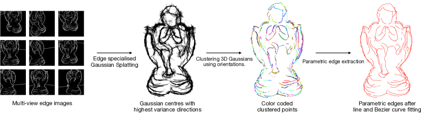
Figure 1: EdgeGaussians: the proposed method learns 3D edge points with an explicit representation where an edge point is cast as a 3D Gaussian centered at that point and the edge direction defines the main orientation of the Gaussian. Left to right: 2D edge maps generated by off-the-shelf detectors [73, 62] are used as supervisory signals to train the 3D edge Gaussians. Once trained, the Gaussian are clustered based on the spatial proximity of their centers and their direction consistency. Parametric edges are fitted on top of these clusters.

3D edge reconstruction from 3D point clouds is free of those limitations and usually follows three steps: classify which 3D points lie on edges, cluster the points belonging to the same edge, and link them [80, 8, 92, 78]. However, the classification is usually hindered by the extreme imbalance between the edge point and the non-edge points, and noisy point clouds can lead to spurious classification. An efficient alternative is to operate directly on a 3D edge point cloud, i.e., a point cloud with points only on the 3D edges.

Such an edge point cloud can be learned from images or 2D edge maps [18, 73] using neural fields [87, 44, 91] trained to represent the 3D edges. Once trained, 3D edge points are sampled from level sets of the neural fields on top of which the 3D edges are fitted. However, such neural fields are computationally expensive and require long training times: recent methods can take 1h30 [91], up to 14h [87] to train on a simple object from the ABC-NEF [91, 41] dataset of CAD models (see Sec. 4 for precise runtimes). Another limitation is the accuracy at which neural implicit fields can represent 3D edges: in theory, the 3D edge points lie on a level set of the field (0 for surface representations [44, 87] and 1 for volumetric ones [91]). In practice though, sampling points on such exact level sets is not feasible due to limited float precision or noise in the training. To compensate for this, the point sampling is done within an $\epsilon$-bound of the level sets [91, 44] but such points do not lie accurately on the 3D edges, requiring post-processing to correct these errors.

To make the 3D edge reconstruction simpler and more efficient while preserving accuracy, we propose to learn an explicit representation of the 3D edge points. It directly learns an edge point cloud, hence bypassing the need for level-set point sampling and post-processing. It also directly learns the point’s edge direction instead of inferring it from the 3D edge points [44], which makes the 3D edge fitting simpler. Last, it is on par with existing learning-based methods and runs much faster, e.g., 30 times faster than EMAP [44] and 17 times faster than NEF [91]. The proposed method defines a 3D edge point as the center of a 3D Gaussian and the edge direction defines the main direction of the 3D Gaussian. Such a representation is geometrically meaningful and is trained in a fast and straightforward manner by adopting the training optimization defined in Gaussian Splats [38]. The optimization is adapted to accommodate the specificities of 3D edge learning mainly the sparsity and the occlusion of the 3D edges. The training remains simple and is supervised with off-the-shelf 2D edge maps [73, 62], as in [44, 91].

To summarize, we make the following contributions: i) We propose a simple, accurate, and extremely efficient method to reconstruct 3D edge points. ii) The proposed method directly learns the oriented 3D points that form the 3D edge point cloud, hence bypassing the delicate and noisy level-set sampling of 3D edge points in existing implicit formulations. iii) Results show that the proposed representation enables 3D edge reconstruction performance better than or at par with previous learning-based methods while running an order of magnitude faster.

2 Related work

3D edge reconstruction methods vary based on the data they are generated from, e.g., images, point clouds, and whether they reconstruct only lines, only curves, or both.

The earliest methods reconstruct 3D lines from images with an SfM approach that detects lines [77, 59, 32, 86, 2], matches them across images based on line descriptors [60, 42, 76, 7], and lifts them to 3D with triangulation [83, 82, 95, 5, 56, 6, 13, 94, 53, 46, 63, 66] or epipolar geometry [27, 28, 29]. The main challenges are matching lines robustly and repetitively detecting lines even when their inconsistent endpoints across views due to occlusions. Existing solutions involve leveraging geometric cues in the scene such as planes [81] and Manhattan frames [67, 16] or replacing hand-crafted steps [77, 7, 76] of the pipeline by their learning counterparts [59, 60, 42, 61]. While recent works [46, 27, 28, 29, 26] have made impressive progress in addressing these limitations, the robustness of the line detection and matching remains a performance bottleneck. These limitations also hold for similar methods reconstructing curves-SfM [36, 68, 65, 37]. This motivates alternative approaches to work around line matching by estimating 3D lines from images using geometric graph optimization on the detected line segments [34, 64], or directly predicting the 3D wireframes in a learning end-to-end manner [97, 49]. A 3D wireframe is a set of 3D lines that define the layout of the scene and form a graph with vertices at edge junctions. Most methods address the 3D line or wireframe mapping problem, with fewer contributions to 3D curve mapping. In this work, we address the 3D mapping of both lines and curves.

Another way to work around the problem of reliable line detection and matching is to directly operate on 3D structures such as depth maps [52], meshes [15], and point clouds obtained from laser scanners [48] or SfM [70]. Given a set of 3D points, most approaches first classify which 3D points lie on edges, cluster the points that lie on the same edge, link them, and fit a parametric edge to each cluster. Each step has hand-crafted [80, 8, 89, 3, 24, 17] and learned variants [92, 78, 93, 25, 98] and some methods operate in an end-to-end manner [78, 93, 15]. One performance bottleneck is the point classification that gets affected by the noise in the point cloud due to laser measurement noise or SfM errors. Another challenge is that the 3D point classification is heavily imbalanced: there are many more non-edge points than edge ones. These challenges are typically addressed by including point filtering steps [14], weighted losses [93, 78] and robust edge parameter estimation [19, 69]. An efficient alternative to the 3D edge point classification is to work on a 3D edge point cloud directly, i.e., a point cloud with points only on the edges of the scene.

Recent works [91, 87, 44] demonstrate how to obtain such 3D edge point clouds from images: they train neural implicit fields that represent the 3D edges and supervise it with the standard rendering loss. The supervisory signals are images [87] or 2D edge maps [91, 44] generated by off-the-shelf detectors [18, 73, 62, 88]. The resulting 3D field is then sampled to get the 3D edge points on top of which the point clustering, linkage, and curve fitting are run. NEF [91] learns an edge density field that represents the probability of a 3D point to lie on a 3D edge. The point sampling then amounts to sampling the 1-level-set. Inspired by VolSDF [90], the edge density is tied to a volumetric density [54] so that NEF can be trained simply with volumetric rendering on the 2D edge maps [73]. NEF is trained with three losses to account for the specificities of 3D edge fields: a sparsity loss to encourage sparse edges, a balancing loss to account for the class imbalance between edge points and non-edge points, and a 3D view consistency loss to account for the occlusions in the supervisory signal. More specifically, NEF renderings display both the visible edges and the occluded ones whereas the 2D edge maps display only the visible ones (See Fig. 2). This consistency loss prevents NEF from wrongly penalizing the rendering when it displays the occluded edges. NEAT [87] adopts a Signed-Distance-Function (SDF) [90] to learn a 3D wireframe field from images. The 3D wireframe points lie on the 0-level set of the field. More recently, EMAP [44] learns a 3D edge field with an Unsigned-Distance-Function (UDF), which is better suited to the problem than SDF that are limited to watertight 3D structures. Compared to NEF [91], they account for the class imbalance and the view-inconsistent occlusions with importance sampling that samples rays along 2D edge and 2D non-edge pixels equally. One common limitation of these methods is their reliance on computationally heavy neural implicit representations to derive the 3D edge point cloud. Also, the point sampling is done within an $\epsilon$-bound of the level sets [91, 44] and such points do not lie accurately on the 3D edges, which require further post-processing.

Instead, we propose to learn directly the 3D edge point cloud with the explicit and extremely efficient Gaussian Splat [38] representation, which is inherently suited to represent edge point clouds: i) the 3D edge points are simply the centers of the learned Gaussians so no point sampling is required; ii) the main direction of the Gaussian defines the 3D edge point direction, which is the direction of the edge it lies on. This greatly simplifies the linkage and clustering step. iii) our method trains an order of magnitude faster than existing methods.

3 3D Edge Reconstruction with 3D Gaussians

3D Gaussians are a relevant alternative representation of 3D edge points that allows for efficient rendering-based training. After training, we revert to the traditional representation with the following mapping: a 3D edge point is the mean of the Gaussian, with the principal axis of the Gaussian as its associated direction. The principal axis of 3D Gaussian is the one with the largest scale. Once the 3D edge point cloud is obtained, the 3D edges are derived with a standard cluster-then-fit approach that first clusters the points into groups that lie on the same edge and then fits an edge to each cluster.

In this section, we first provide an overview of the original 3D Gaussian Splatting framework introduced in [38]. We then present an adaption of the splatting framework for the 3D edge reconstruction using multi-view 2D edge maps. Last, we describe how edges are fitted from the proposed explicit representation.

3.1 Preliminaries: 3D Gaussian Splatting (3DGS)

3D Gaussian Splatting [38] represents the scene using a set of 3D Gaussians. The mean $\mu\in\mathbb{R}^{3}$ of the Gaussian defines its position, and the scale and the orientation of the Gaussian are defined by its covariance matrix $\Sigma\in\mathbb{R}^{3\times 3}$. A 3D Gaussian centered at $\mu$ is defined as:

$$G(x)=e^{-\frac{1}{2}(x-\mu)^{T}\Sigma^{-1}(x-\mu)}\enspace.$$ (1)

Each Gaussian also has an opacity attribute $\alpha$ and a color attribute $c$ represented by spherical harmonic coefficients. All the Gaussian’s parameters are differentiable and are trained by rendering the 3D Gaussians and comparing the rendered images to the original images. The loss is a combination of the $\mathcal{L}_{1}$ loss and the Difference of Structural Similarity loss [79] (D-SSIM) $\mathcal{L}_{\text{SSIM}}$ between the two, weighted by $\lambda\in\mathbb{R}$:

$$\mathcal{L}=\lambda\mathcal{L}_{1}+(1-\lambda)\mathcal{L}_{\text{D-SSIM}}\enspace.$$ (2)

The rendering first projects the 3D Gaussians to 2D splats [99]. The color of a pixel in the rendering is derived by selecting the Gaussians which splats overlap with the pixel, ordering them based on their depth, and $\alpha$-blending their colors. To optimize the covariance matrix $\Sigma$ while maintaining its positive-semi definiteness, it is decomposed into a rotation matrix $R\in\mathbb{R}^{3\times 3}$ and a diagonal scaling matrix $S\in\mathbb{R}^{3\times 3}$, such that $\Sigma=RSS^{T}R^{T}$.

The representation is initialized with Gaussians centered at a sparse set of points, e.g., obtained from SfM [70]. The set of Gaussians in the scene is dynamically controlled by duplicating, splitting, and culling Gaussians based on various criteria - the important ones being 1) culling low-opacity Gaussians; and 2) duplicating/splitting Gaussians that are in a region that needs densification, or is a complex 3D surface requiring more Gaussians.

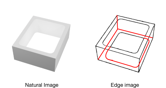
Figure 2: Occlusions for 3D edges. The red edges are the occluded edges absent from the supervisory 2D edge maps. This occlusion is inherited from the occlusion in the natural image (left) from which the 2D edge maps are inffered [73, 62]. Yet, these edges are present in the rendering of the 3D edge representation, which is the desired behavior.

3.2 Gaussian Splatting for Edge Images

The original Gaussian Splatting previously described is designed to reconstruct scenes in the wild so that novel views can be accurately and efficiently rendered. It is agnostic to the content of the images so it can train on 2D edge maps [18, 73, 62, 88] in a straightforward manner. Such an off-the-shelf training produces reasonable renderings. However, the properties of 3D edges, such as their geometry and their sparsity, and the inconsistencies between the 3D Gaussian renderings and the 2D edge maps used as supervisory signals require some adaptation of 3DGS, which we describe next.

Before, note that 3D edges are colorless by nature so we discard the spherical harmonic parameters used to model colors and view-dependent appearance, which significantly reduces the number of parameters [21] and contributes to our method’s efficiency.

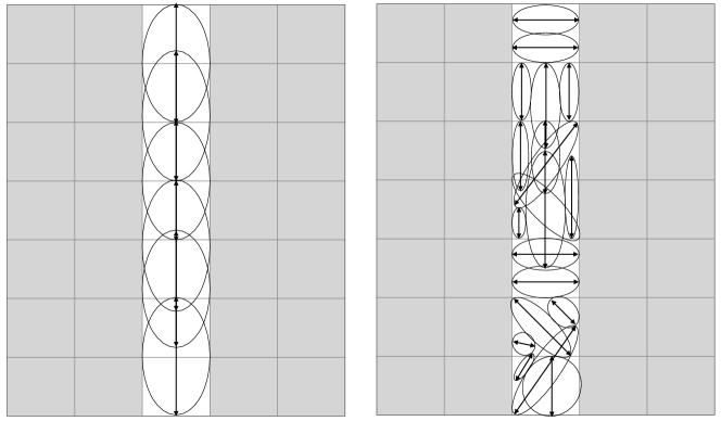
Figure 3: The two geometric criteria for the learned 3D Gaussians. Given the 3D edge point cloud, the 3D edges are derived by first clustering the points that belong to the same edges and then fitting an edge to each cluster. To enable such clustering, the Gaussians associated with two 3D edge points that lie on the same edge and that are neighbors must be spatially close and have similar directions (left) (see Sec. 3.2). Gaussians without the direction constraints are illustrated on the right. The white pixels of the grid here show edge pixels while grey ones show background.

3D edge sparsity and incomplete supervision.  Natural images typically depict the surfaces of the scene, which is a dense 3D geometry, so there are relatively few empty spaces. This is the opposite of 2D edge maps that depict 3D edges that are inherently sparse. As already observed in previous works [44, 91], such an extreme imbalance in the pixel distribution can hinder the training convergence. For example, since edge maps consist mostly of zero-value pixels where no 3D edge reprojects and few pixels with non-zero values, the training could converge to valid but degenerate sets of Gaussians such as an empty set of Gaussians or Gaussians with only background color.

Another issue lies in the supervisory signal: the proposed method, as well as previous works [91, 44], supervise their training with 2D edge maps generated by off-the-shelf detectors [73, 62]. The edge maps are generated from natural images with occlusions that the edge maps inherit even when the occlusions do not affect the 3D edges. We illustrate this phenomenon in Fig. 2: the supervisory edge map is generated from the natural image (left) and comprises only the visible edges (black edges on the right). However, the rendering of the 3D edges learned by the trained representations do show the occluded edges (red), which is the desired behavior. Naively training the model with the standard rendering loss would penalize the model for rendering the occluded edges, i.e., the red edges.

To address these issues, NEF [91] weights the rendering loss based on the pixel’s probability to be an edge, i.e., the pixel’s intensity in the edge map. This penalizes the edge pixels more than the non-edge pixels for which the supervisory signal is less reliable. However, this reduces the supervisory signal on occluded edges and the trained Gaussians would result in incomplete reconstructions: the 3D edges seen only by few edge maps would get discarded because their opacity would be too low. EMAP [44] works around this limitation with importance sampling that samples rays uniformly between edge and non-edge pixels. We adopt a similar strategy except that we sample uniformly at random between edge and non-edge pixels instead of rays to compute the projection loss.

This is derived by simply masking the $\mathcal{L}_{1}$ loss between a rendered image $\hat{I}$ and a training image $I$ as follows:

$$\mathcal{L}_{\text{proj}}=\text{average}\left(\mathcal{M}\odot|\hat{I}-I|\right)\enspace$$ (3)

where $\odot$ is Hadamard product and $\mathcal{M}$ is a 2D binary mask with values 1 at all edge pixels and at an equal number of randomly selected background pixels. Also, we discard the SSIM term in Eq. 2.

Learning oriented edge points as Gaussians.  The learned Gaussians should be such that the resulting edge points not only lie on the 3D edges but also are suitable for the subsequent edge fitting. As detailed in Sec. 3.3, we adopt a cluster-then-fit strategy that first clusters the points into groups that lie on the same edge and then fits an edge to each cluster. The clustering is cast as a simple graph traversal where the vertices are the oriented edge points: the vertex’s position is the Gaussian’s center and the vertex’s direction is the Gaussian’s principal direction. To allow such clustering to identify edges, the Gaussians should comply with two criteria illustrated in Fig. 3: i) the Gaussians belonging to the same edge should have centers that are spatially close; ii) the Gaussians belonging to the same edge should have a similar direction, i.e., their principal axes should be colinear. The second criterion is enforced by constraining the principal direction of the Gaussian with the largest axis to align with the direction of the edge it lies upon. A simple way to implement such a constraint is to encourage the principal axis of a 3D Gaussian to point towards its $k$ nearest neighbors in 3D, $k$ being a hyperparameter. Mathematically, we enforce the magnitude of the dot product between the principal axes of neighboring Gaussians to be close to 1. Given $N$ 3D Gaussians indexed between $1$ and $N$, let $\mu_{i}$ and $d_{i}$ be respectively the center and the principal direction of the $i^{th}$ Gaussian, and let $i_{1},...,i_{k}$ be the indices of the neighbors, we enforce the constraint with the following loss:

$$\mathcal{L}_{\text{orient}}=1-\frac{1}{N}\left(\sum_{i=1}^{N}\frac{1}{k}\sum_{j=1}^{k}|d_{i}^{T}d_{i_{j}}|\right)$$ (4)

We also regularize the Gaussians to have an ellipsoidal shape instead of spherical or disc-like shape so that identifying the principal direction of the Gaussian, i.e., the largest axis, is computationally more stable. For example, in the extreme case where the Gaussian is a perfect sphere, all directions would be the principal directions since they would have the same scale. The regularization encourages the largest axis of the Gaussian to be distinctive enough, which amounts to enforcing the ratio between the largest scale and the next one to be large:

$$\mathcal{L}_{\text{shape}}=\frac{1}{N}\sum_{i=1}^{N}\frac{{}^{2}s_{i}}{{}^{1}s_{i}}$$ (5)

where ${}^{1}s_{i}$ and ${}^{2}s_{i}$ are the scales of the largest and the second largest axes of the $i^{th}$ Gaussian.

The final loss is the sum of the three terms weighted by $\lambda_{1},\lambda_{2}\in\mathbb{R}$:

$$\mathcal{L}=\mathcal{L}_{\text{proj}}+\lambda_{1}\mathcal{L}_{\text{orient}}+\lambda_{2}\mathcal{L}_{\text{shape}}$$ (6)

An example of the resulting 3D Gaussians is shown in Fig. 1 where the length of the Gaussian’s principal direction is increased for visualization purposes.

3.3 Edge Fitting

Given a 3D edge point cloud, there are mainly two edge fitting strategies: the fit-then-cluster approach used in NEF [91] that operates in a multi-RANSAC [20] fashion. The clusters are simply the inlier supports of each edge. The second strategy is the cluster-then-fit approach, also used in EMAP [44]: it first clusters the points belonging to the same edges and then fits an edge to each cluster. We adopt the latter strategy as the qualitative results of NEF [91] show that the first strategy sometimes ignores the local geometry of the 3D edge points. For example, curves get fitted by lines, and neighboring points belonging to the same edge are inliers to different edges.

Clustering points into edges.  A common strategy to cluster points is to adopt a graph-traversal approach where points form the vertices of the graph and an edge exists between two vertices only if they are spatially close [55, 22]. Clustering the points into their supporting edges then amounts to solving a graph traversal problem. This simple solution is usually made robust by integrating a smoothness constraint between neighboring points [57]: two vertices are connected not only if they are spatially close but if their direction is also similar. This is what motivates the two constraints on the Gaussian’s orientation previously described in Eq. 4 and  Eq. 5. We adopt this graph traversal approach that is also used in EMAP [44] and has proven to be effective.

Given the trained Gaussians, we define the graph as follows. The vertices of the graph represent oriented edge points: the vertex’s position is the Gaussian’s center and the vertex’s direction is the Gaussian’s principal direction. Vertices are neighbors if they are spatial neighbors and if they have similar orientations. During traversal, we add a third orientation criterion for robustness: a new vertex is added to the current path / cluster only if its orientation is consistent with the path’s global direction, i.e., the edge direction. This is measured by comparing the direction of the path and the direction between the new vertex and the one last added to the path. These two directions should be close. This favors sharper clustering around corners where the learned direction can get smooth. For all orientation tests, we use a single orientation threshold $\theta$. The graph traversal results in clusters of points belonging to the same edge. We then fit edges to the resulting clusters in the form of line segments and cubic Bezier curves.

Method	Detector	Modal	Acc$\downarrow$	Comp$\downarrow$	R5$\uparrow$	R10$\uparrow$	R20$\uparrow$	P5$\uparrow$	P10$\uparrow$	P20$\uparrow$	F5$\uparrow$	F10$\uparrow$	F20$\uparrow$
LIMAP [46]	LSD	Line	9.9	18.7	36.2	82.3	87.9	43.0	87.6	93.9	39.0	84.3	90.4
	SOLD2	Line	5.9	29.6	64.2	76.6	79.6	88.1	96.4	97.9	72.9	84.0	86.7
	PiDiNeT†	Curve	11.9	16.9	11.4	62.0	91.3	15.7	68.5	96.3	13.0	64.0	93.3
NEF [91]	PiDiNeT	Curve	15.1	16.5	11.7	53.3	93.9	12.3	61.3	95.8	12.3	51.8	88.7
	DexiNed	Curve	21.9	15.7	11.3	48.3	93.7	11.5	58.9	91.7	10.8	42.1	76.8
	PiDiNeT	Edge	9.2	15.6	30.2	75.7	89.5	35.6	79.1	95.4	32.4	77.0	92.2
EMAP [44]	DexiNed	Edge	8.8	8.9	56.4	88.9	94.8	62.9	89.9	95.7	59.1	88.9	94.9
	PiDiNeT	Edge	11.7	10.3	17.1	73.9	83.1	26.0	87.2	92.5	20.58	79.3	86.7
Ours	DexiNed	Edge	9.6	8.4	42.4	91.7	95.8	49.1	94.8	96.3	45.2	93.7	95.7

Table 1: 3D Edge Reconstruction on ABC-NEF [91]. Overall, the proposed method is on par with the baselines and slightly better than the implicit representations NEF [91] and EMAP [44] under the 10mm and 20mm error thresholds. Under the 5mm threshold, the geometry-based LIMAP [46] outperforms most methods. We explain the lower performance of our method under this threshold by the bias in the 2D edge maps [73, 62] used as a supervisory signal. The baselines results are taken as provided by Table 1 in EMAP [44].

Parametric Edge Fitting.  The previous clustering generates groups of points that belong to the same edges on top of which we estimate a parametric representation of the edges. These edges can be either 3D lines or 3D curves, each having a different parametric representation so one must select which parametric model to fit on each cluster. To select between the two, we fit both a line and a curve on a given cluster and use the residuals’ error to select the best model.

Let $e_{\text{c}}$ and $e_{\textit{l}}$ be the average residual error of the curve and line models respectively. We select the curve model if the error $e_{\text{c}}$ is smaller than a fraction $\delta$ of the line residual error, i.e., $e_{\text{c}}\leq\delta e_{\textit{l}}$. The parameter $\delta$ can be tuned to control the fraction of lines and curves in the output. As shown in the qualitative results (Fig. 4), this strategy is more effective than the ones adopted in NEF [91] and EMAP [44]. NEF [91] first approximates all edges with 2-control-points Bezier curves, i.e., 3D lines, and uses the estimated control point to further optimize the models into 3D curves when needed. This approach produces several degenerate curve configurations, especially close to the corners. As for EMAP [44], it first fits 3D lines, filters out their inlier points, then fits 3D curves on top of the remaining points. This has the disadvantage of making the line fitting agnostic to the presence of curves so a large fraction of curves get fitted by lines instead.

4 Evaluation

We evaluate the proposed method against image-based edge reconstruction methods following the evaluation setup in EMAP [44]. Results show that our method reaches mapping performance on par with the state-of-art while running an order of magnitude faster. The rest of this section describes the evaluation setup and reports the results.

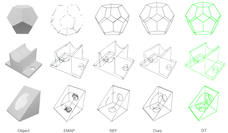
Figure 4: Qualitative results on ABC-NEF [91]. The proposed method captures curves and lines accurately but can be marginally incomplete. EMAP [44] is either slightly less complete than the proposed method or predicts extra edges. NEF [91] produces correct edges but exhibits knots observed around corners on many occasions.

4.1 Experimental Setup

Datasets.  We follow the quantitative evaluation defined in EMAP [44] that runs on two datasets: ABC-NEF [91, 41] and DTU [35]. The evaluation runs on the data released by EMAP [44], which includes 2D edge maps [73, 62] used for training, and with their released evaluation code. We also report qualitative results on the Replica dataset [72] in the supplementary material.

The ABC-NEF [91] dataset is a subset of the ABC dataset [41] curated specifically for the task of 3D edge mapping. It holds 115 CAD models, ground-truth parametric edges, and 50 views rendered from around the object. We use the subset of ABC-NEF selected by the authors of EMAP [44] that keeps 82 out of the 115 CAD models obtained after filtering out models with cylinders and spheres - ones that are inconsistent with edge observations. The DTU dataset [35] comprises multi-view images of everyday objects captured from fixed frontal viewpoints. We evaluate on the 6 DTU scenes for which the EMAP [44]’s authors provide pseudo-ground-truth 3D edge points. The pseudo-ground-truth is obtained by projecting 3D points measured by a structured-light scanner [1] onto the images and by filtering out the points that do not project to 2D edges [10]. Although we perform at par or better than the baselines on DTU, we observe that the pseudo-ground-truth introduces biases in the evaluation and we illustrate them in the qualitative results. Finally, as in [44], we report qualitative results on three scenes of the Replica dataset [72] that comprises high-quality reconstructions. We do not run quantitative evaluation on Replica for it does not provide any ground-truth edges.

Baselines.  We evaluate the line-SfM-based method LIMAP [46] that sets the state-of-the-art in geometry-based 3D line reconstruction and the 3D wireframe learning method NEAT [87]. We also evaluate the state-of-the-art 3D line / curve mapping methods NEF [91] and EMAP [44]. Following [44], NEAT [87] is not evaluated on ABC-NEF [91]: the authors observe that it often fails to train on the textureless renderings of the CAD models. The qualitative results we report are generated with the code and the weights released by the authors of the various baselines. For EMAP [44], at the time of writing, running the released code with the recommended configurations does not yield the exact same results as the ones shown in the paper or the website. We therefore report the results run on checkpoint versions graciously provided by the authors. The quantitative results for the baselines are reported from [44].

Metrics.  The ground-truth edges for the ABC-NEF [91] dataset are provided so parametric edges can be evaluated quantitatively. The evaluation defined in [44] samples points along the predicted parametric edges and compares those points against points sampled at the same resolution on the ground-truth edges to compute the metrics. The accuracy defines the mean distance from the predicted points to the closest ground-truth points, and the completeness defines the mean distance between the ground-truth points and their nearest predicted point. For these two metrics, the lower the better. The precision at a distance threshold $\tau$ (P($\tau$)) measures the percentage of predicted points with at least one ground-truth point within distance $\tau$. Symmetrically, the recall (R($\tau$)) measures the percentage of ground-truth points for which a predicted point is within the distance threshold $\tau$. For precision and recall, the higher the better. We report the metrics for $\tau$ in 5, 10, and 20 millimeters (mm). Note that the used error thresholds are quite strict, as ABC-NEF [91] objects are scaled so that the largest edge of the bounding box measures 1 meter (m). We also compare the running times of the different neural implicit representation methods to show the advantage of the explicit representation adopted in this paper. We do not report the Edge Direction Consistency metric (Norm) [44] as, at the time of the writing, the theoretical definition and the implementation of that metric are not available.

Although these metrics provide a meaningful evaluation of the reconstruction quality, they do not account for all the performance aspects of the 3D edge reconstruction. For example, duplicate edge reconstructions that lie close to a ground-truth edge are not penalized. This is especially important on the DTU dataset which pseudo-ground-truth 3D edge points do not lie exactly on the 3D edges but along the 3D edges, as illustrated in Fig. 5.

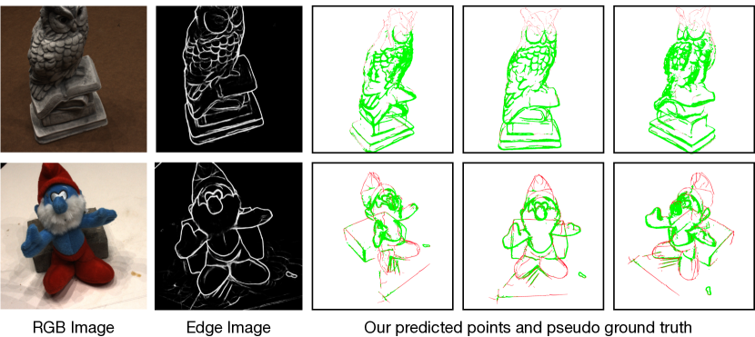
Figure 5: Qualitative results and pseudo-ground-truth on DTU [35]. We visualize our method (red) and the pseudo-ground-truth edge points (green) generated in [44] by projecting ground-truth 3D points onto an image and filtering the ones that fall out of 2D edges [10]. Note that our method gets penalized in precision when it predicts geometrically correct 3D edges that are missing from the pseudo-ground-truth, e.g., the top of the smurf and the howl. Also, the pseudo-ground-truth contains thick patches of points that make it difficult for well-predicted edges to get a high recall. Still, our method faithfully reconstructs the 3D parametric edges of the objects.

Implementation details  On ABC-NEF [91], we initialize our method with Gaussians centered at 10000 points randomly sampled in a unit cube. We use constant color and optimize for the positions, scales, and orientations of the Gaussian parameters. We use $k=4$ as the number of nearest neighbors for computing$\mathcal{L}_{\text{orient}}$ 4. The weights of the loss function in Eq. 6 are $\lambda_{1}=0.5$ and $\lambda_{2}=0.25$ when using the DexiNed [62] 2D edge maps. With PidiNet [73], we use a slightly lower value for $\lambda_{2}=0.1$ to account for the thicker edges. Further details about the initialization parameters can be found in the supplementary. During clustering, the alignment threshold is $\theta=0.8$ on ABC-NEF [91], which have clean straight lines, and $\theta=0.6$ on DTU [35] to account for the higher curvature of the shapes. During the parametric edge fitting, we fit a curve whenever the curve residual error is $\delta=0.5$ lower than the line residual error. Runtimes are reported for learning-based methods that all run on an Nvidia A100 GPU.

4.2 Results

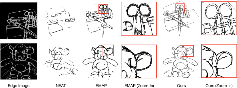
Figure 6: Qualitative results on DTU [35]. Comparison of the proposed 3D reconstruction method against baselines. NEAT [87] produces partially complete reconstructions with lines only. The EMAP [44] edges are more complete but there are duplicate edge predictions for a single target edge in 3D, while our reconstruction is much cleaner with mostly a single predicted edge boundary (see zoom-ins).

Scan	LIMAP [46]		NEF [91]		NEAT [87]		EMAP [44]		Ours
	R5$\uparrow$	P5$\uparrow$	R5$\uparrow$	P5$\uparrow$	R5$\uparrow$	P5$\uparrow$	R5$\uparrow$	P5$\uparrow$	R5$\uparrow$	P5$\uparrow$
37	75.8	74.3	39.5	51.0	63.9	85.1	62.7	83.9	83.0	80.3
83	75.7	50.7	32.0	21.8	72.3	52.4	72.3	61.5	81.6	65.8
105	79.1	64.9	30.3	32.0	68.9	73.3	78.5	78.0	78.3	75.9
110	79.7	65.3	31.2	40.2	64.3	79.6	90.9	68.3	87.3	60.0
118	59.4	62.0	15.3	25.2	59.0	71.1	75.3	78.1	84.9	76.6
122	79.9	79.2	15.1	29.1	70.0	82.0	85.3	82.9	92.3	84.8
Mean	74.9	66.1	27.2	33.2	66.4	73.9	77.5	75.4	84.6	73.5

	ABC-NEF [91]	DTU [35]
NEF [91]	1:26	1:50
NEAT [87]	14:13	8:38
EMAP [44]	2:30	12:00
Ours	0:05	0:05

Table 2: Left: 3D Edge Reconstruction on DTU [35]. Comparison of precision (P) and recall (R) under 5mm error. The scenes are scaled to a bounding box of a maximum side of 1 meter. Right: Average Runtimes of implicit representation methods in ‘hour:minutes’. The 3D edge reconstruction of the proposed method performs better or is at par with the learning-based baselines NEF [91], EMAP [44] and NEAT [87] and runs an order of magnitude faster.

Evaluation on ABC-NEF [91].  We report the quantitative evaluation in Tab. 1 and the qualitative results in Fig. 4. Overall, the proposed method is on par or slightly better than the implicit-representations-based NEF [91] and EMAP [44] and runs respectively 17 and 30 times faster (LABEL:{tab:dtu_and_runtime}-right). This supports that the proposed explicit representation enables efficient 3D edge reconstruction while preserving accuracy.

The accuracy and the completeness of our method are on par with EMAP [44] and significantly better than NEF [91]. However, the accuracy of all learning-based methods falls behind the accuracy of the geometry-based LIMAP [46]: it predicts points closer to the ground-truth ones although its completeness has room for improvement. This is indicated by the relatively lower completeness and recall metrics. Note that the ABC-NEF [91] CAD models are scaled to fit the unit cube so objects span one meter, which makes the millimeter (mm) error thresholds used in the evaluation extremely harsh. LIMAP [46] demonstrates impressive results followed by EMAP [44] that performs better than the proposed method under the 5mm error threshold although this trend is inverted under the 10mm and 20mm error thresholds. We note that the performance of the proposed method when supervised with the 2D edge maps generated by the PidiNet [73] detector is slightly worse than with DexiNed [62], although it remains very competitive with all baselines.

We explain the lower performance of our method under the 5mm error threshold by the bias that exists in the 2D edge maps used as a supervisory signal during training. This bias is introduced by the off-the-shelf detectors [73, 62] that generate 2D edges typically thicker than the projection of the ground-truth 3D edges (See example in Fig. 5). The learned Gaussians remain valid as long as they project onto the 2D edge maps, which is the case for 3D Gaussians lying close to but not on the 3D edges. In fact, the thicker the 2D edges, the farther away from the 3D edges can the valid Gaussians be. We verify this hypothesis visually and observe that even edge reconstructions with poor metrics exhibit 3D edge points that are close to the ground-truth edge. Independently of the reported results, we approximately quantify this bias by fitting the predicted 3D edge points to the ground-truth one and measure that the 2D edge map bias induces an error in the 3D Gaussian position of $\sim$0.5% of the scene size, which is $\sim$5mm for the 1 meter-wide objects in the ABC-NEF [91].

Evaluation on DTU [35].  The quantitative results are reported in Tab. 2-left and the qualitative results in Fig. 5 and Fig. 6. On each of the 6 DTU scans, our method either outperforms or is at par with the baselines. However, we observe biases in the evaluation introduced by the pseudo-ground-truth generation process. As mentioned in Sec. 4.1, the pseudo-ground-truth is obtained from a 3D point cloud by filtering out the points that do not project to edges on the 2D edge maps [10]. However, the edge maps exhibit edges [73, 62] thicker than the projection of the actual ground-truth 3D edges (Fig. 5). So the 3D points that get labeled as pseudo-ground-truth edge points are not only the points lying on the ground-truth edges but also the points within an $\epsilon$-bound on the edge, and the range of the bound is a function of the 2D edge map thickness and the distance between the object and the camera. We refer to this bias as the thickness bias. Another bias originates from the occlusions in the 2D edge maps that cause some 3D points to be incorrectly labeled as non-edge points. Fig. 5 illustrates these biases and compares the pseudo-ground-truth points (green) to the points sampled on the parametric edges predicted by our method (red). It can be clearly seen that our parametric edges are more complete than the pseudo-ground-truth points. Several predicted edges, for example in the hat and legs of the smurf soft toy, are not covered by the ground-truth, which illustrates the occlusion bias. This bias hinders the precision of our method even though the predictions are correct. The thickness bias is illustrated by the relatively thicker pseudo-ground-truth curves in green compared to the thinner edge predictions in red. This bias not only penalizes the recall of our method but also incorrectly favors methods that reconstruct duplicate edges along the ground-truth edges, which is undesirable as it makes the reconstruction noisier. Fig. 6 illustrates the edges predicted by our method and the baselines and show examples where EMAP [91] predicts duplicate edges whereas our method generates single and precise edges. As for the runtime, our method is as efficient as on the ABC-NEF [91] dataset and runs 22 times faster than NEF [44] and more than a hundred times faster than EMAP [44] (Tab. 2-right).

5 Conclusion

In this work, we propose a method for 3D edge reconstruction from images that explicitly learn the 3D edge points on top of which the 3D edges are fitted. The explicit representation is simple and casts 3D edge points as 3D Gaussians and the edge direction as the principal axis of the Gaussians. Such a representation allows for efficient rendering-based training supervised with off-the-shelf 2D edge maps. Results show the efficiency of the proposed explicit representation that enables 3D edge reconstruction performances on par with previous implicit representations yet runs an order of magnitude faster. While the off-the-shelf 2D edge maps make for a relevant supervisory signal, we observe that they can introduce bias in the training or the evaluation, which calls for investigating better supervision in the future.

Supplementary Material

Appendix A provides implementation details about the training of the edge-specialized Gaussian Splatting in addition to those provided in the main paper. Appendix B shows qualitative results over the test split of the Replica [72] dataset defined by the authors of EMAP [44]. Fig. 10 illustrates the limitations and failure cases of our method.

Appendix A Additional Implementation details

Gaussian Parameters Initialization.  At the beginning of the training, the Gaussians are initialized as follows. Gaussian Position: The CAD models of the ABC-NEF [91] dataset comprises texture-less objects on which SfM [70] generates extremely sparse or no point reconstruction at all. We therefore initialize the Gaussian means with 10000 randomly sampled points inside a unit cube. For scenes from the DTU [35] and Replica [72] datasets, we use the SfM [70] points as initialization. We note that the method also works with similar accuracy with the random point initialization. On the Replica [72] scene, the set of points is larger as the scene is larger and contains more elements. Scenes across all datasets are scaled so that the scene fits in a box which largest side is 1 meter (m). Gaussian Scale: We use a constant initial value of 0.004 for all datasets. Gaussian Opacity: We use a constant initial value of 0.08 for all datasets. Gaussian Orientation: Random unit quaternions are used as initial values for all Gaussians.

Training Strategy.  We train the model for 500 epochs. For the first 30 epochs, we only train the position parameters so that the scale and the orientation of the Gaussian do not compensate for its incorrect position during rendering. Thus the training constrains the Gaussian’s position, i.e.mean, to lie on 3D edges. We cull the Gaussians based on opacity and duplicate the ones with high positional gradients at regular intervals similar to the original work [38]. The learning rates of different parameters are as follows. Position: starting with $1e^{-3}$, scaled with a factor of 0.75 every 10 epochs, 5 times. Scale: $2e^{-4}$ constant. Opacity: $3e^{-2}$ constant. Orientation: $1e^{-3}$ constant.

Appendix B Qualitative Results over Replica

Fig. 7 to 9 show the results for the scenes room_0, room_1, room_2 of the Replica [72] dataset. The results show that our method produces edges with a higher completeness than EMAP [44]. Also, EMAP [44] predicts clusters of duplicate edges close to the ground-truth edge, which is not a desirable result as it makes the reconstruction less sharp. Overall, our method produces clean single edges that are more complete. However, in some cases, EMAP [44] produces geometrically accurate lines, which our method captures as incomplete curves. Fig. 8 shows one such example. Although this can be partially addressed by adjusting the parameter $\delta$ involved in the model selection when fitting a line or a curve, this could be seen as a current limitation of our method.

Appendix C Limitations / Failure Cases

We now review the limitations of the proposed method.

Fine structures.  In the qualitative results, we observe that the proposed method can not always reconstruct the edges of thin or near planar structures. Fig. 10 shows 3 such examples on the ABC-NEF [91] dataset where the method generates either broken curves or single edges in presence of fine multiple edges. The object on the right in Fig. 10 further has edges inside the object that are not detected in the 2D edge maps, i.e., there is no supervision for those edges, hence it is not possible to map them in 3D.

Large Scale Scenes.  The method has been tested with bounded scenes scaled within a unit cube. Scaling robustly to unbounded scenes is left for future work.

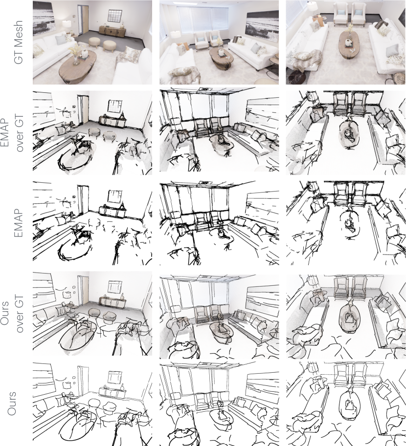
Figure 7: Replica [72] room_0 : Qualitative result showing edges produced by our method and EMAP [44]. In general it can be observed that EMAP [44] has several duplicate / dense sets of edges close to ground-truth edges whereas our method produces clean single edges.

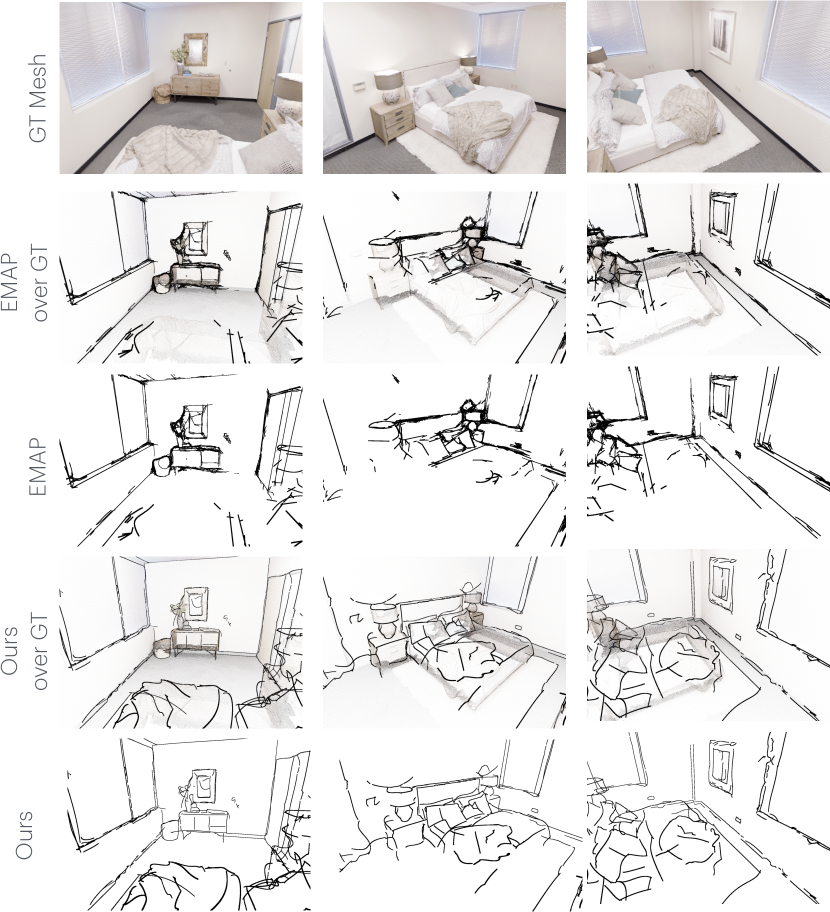
Figure 8: Replica [72] room_1 : Qualitative result showing three different views of edges produced by our method and EMAP [44]. In general it can be observed that EMAP [44] has several duplicate / dense sets of edges close to ground-truth edges, while our method produces clean single edges. However, EMAP [44] produces more accurate lines for some geometric edges, for example, on the window pane.

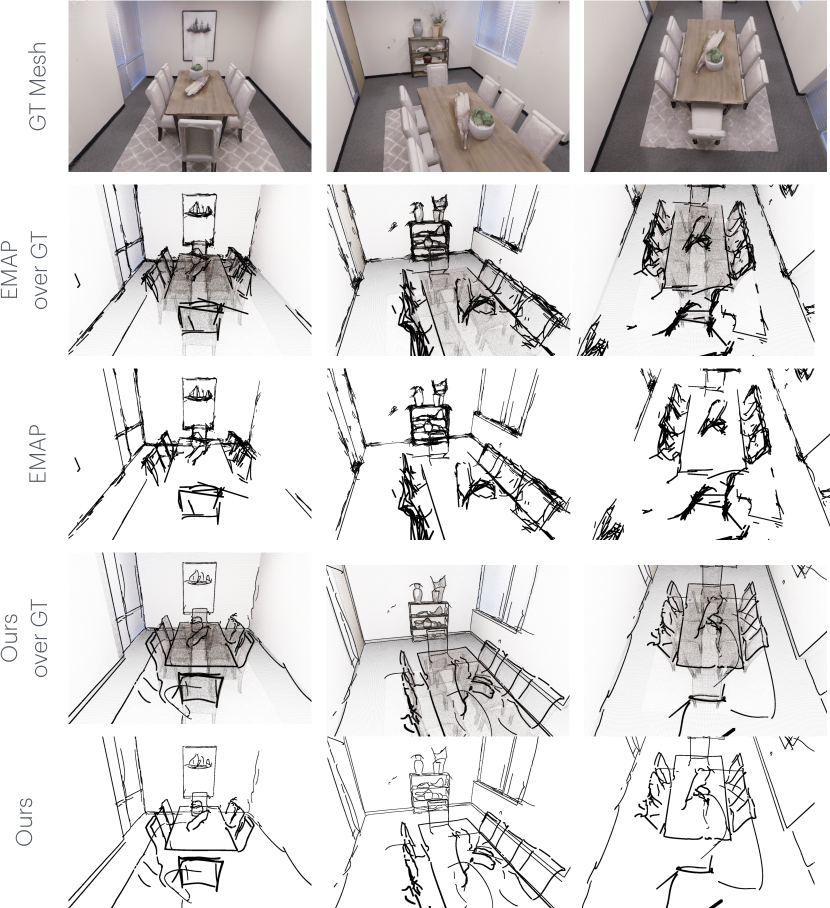
Figure 9: Replica [72] room_2 : Qualitative result showing edges produced by our method and EMAP [44]. In general it can be observed that EMAP [44] has several duplicate / dense sets of edges close to ground-truth edges, while our method produces clean single edges.

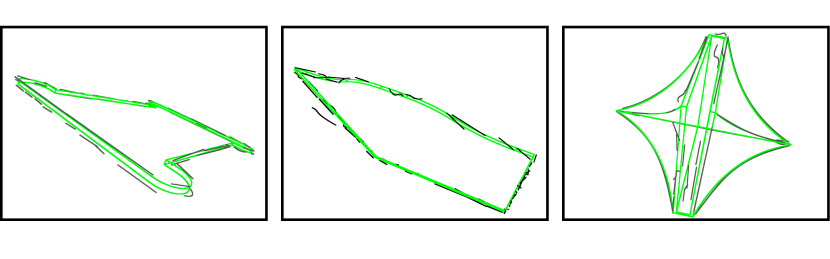
Figure 10: Failure cases : Scans 00009685, 00002412 and 00003884 (left to right) on the ABC-NEF [91]. The edges predicted by our method are shown in black and the ground-truth ones in green. These examples are challenging because they show extremely thin structures: the projection on two distinct parallel and close 3D edges can get projected into a single edge in several views of the supervisory 2D edge maps [73, 62]. Another example where the proposed method is incomplete (right) is when the object has 3D edges inside the structure that are not detected by the 2D edge detectors. Then, there is no supervisory signal for those 3D edges.

(glossaries) Package glossaries Warning: No “printglossary or “printglossaries found. Ω(Remove “makeglossaries if you don’t want any glossaries.) ΩThis document will not have a glossary

References

- [1] Henrik Aanæs, Rasmus Ramsbøl Jensen, George Vogiatzis, Engin Tola, and Anders Bjorholm Dahl. Large-scale data for multiple-view stereopsis. International Journal of Computer Vision, 120:153–168, 2016.
- [2] Hichem Abdellali, Robert Frohlich, Viktor Vilagos, and Zoltan Kato. L2d2: Learnable line detector and descriptor. In 2021 International Conference on 3D Vision (3DV), pages 442–452. IEEE, 2021.
- [3] Syeda Mariam Ahmed, Yan Zhi Tan, Chee Meng Chew, Abdullah Al Mamun, and Fook Seng Wong. Edge and corner detection for unorganized 3d point clouds with application to robotic welding. In 2018 IEEE/RSJ international conference on intelligent robots and systems (IROS), pages 7350–7355. IEEE, 2018.
- [4] Marc Alexa, Johannes Behr, Daniel Cohen-Or, Shachar Fleishman, David Levin, and Claudio T. Silva. Computing and rendering point set surfaces. IEEE Transactions on visualization and computer graphics, 9(1):3–15, 2003.
- [5] Caroline Baillard, Cordelia Schmid, Andrew Zisserman, and Andrew Fitzgibbon. Automatic line matching and 3d reconstruction of buildings from multiple views. In ISPRS Conference on Automatic Extraction of GIS Objects from Digital Imagery, volume 32, pages 69–80, 1999.
- [6] Adrien Bartoli and Peter Sturm. Structure-from-motion using lines: Representation, triangulation, and bundle adjustment. Computer vision and image understanding, 100(3):416–441, 2005.
- [7] Herbert Bay, Vittorio Ferraris, and Luc Van Gool. Wide-baseline stereo matching with line segments. In 2005 IEEE Computer Society Conference on Computer Vision and Pattern Recognition (CVPR’05), volume 1, pages 329–336. IEEE, 2005.
- [8] Dena Bazazian, Josep R Casas, and Javier Ruiz-Hidalgo. Fast and robust edge extraction in unorganized point clouds. In 2015 international conference on digital image computing: techniques and applications (DICTA), pages 1–8. IEEE, 2015.
- [9] Assia Benbihi, Stéphanie Arravechia, Matthieu Geist, and Cédric Pradalier. Image-based place recognition on bucolic environment across seasons from semantic edge description. In 2020 IEEE International Conference on Robotics and Automation (ICRA), pages 3032–3038. IEEE, 2020.
- [10] Andrea Bignoli, Andrea Romanoni, Matteo Matteucci, and Politecnico di Milano. Multi-view stereo 3d edge reconstruction. In 2018 IEEE Winter Conference on Applications of Computer Vision (WACV), pages 867–875. IEEE, 2018.
- [11] Waldemar Celes and Frederico Abraham. Texture-based wireframe rendering. In 2010 23rd SIBGRAPI Conference on Graphics, Patterns and Images, pages 149–155. IEEE, 2010.
- [12] Waldemar Celes and Frederico Abraham. Fast and versatile texture-based wireframe rendering. The Visual Computer, 27:939–948, 2011.
- [13] Manmohan Chandraker, Jongwoo Lim, and David Kriegman. Moving in stereo: Efficient structure and motion using lines. In 2009 IEEE 12th International Conference on Computer Vision, pages 1741–1748. IEEE, 2009.
- [14] Siheng Chen, Dong Tian, Chen Feng, Anthony Vetro, and Jelena Kovačević. Fast resampling of three-dimensional point clouds via graphs. IEEE Transactions on Signal Processing, 66(3):666–681, 2017.
- [15] Kseniya Cherenkova, Elona Dupont, Anis Kacem, Ilya Arzhannikov, Gleb Gusev, and Djamila Aouada. Sepicnet: Sharp edges recovery by parametric inference of curves in 3d shapes. In Proceedings of the IEEE/CVF Conference on Computer Vision and Pattern Recognition, pages 2727–2735, 2023.
- [16] James Coughlan and Alan L Yuille. The manhattan world assumption: Regularities in scene statistics which enable bayesian inference. Advances in Neural Information Processing Systems, 13, 2000.
- [17] Kris Demarsin, Denis Vanderstraeten, Tim Volodine, and Dirk Roose. Detection of closed sharp edges in point clouds using normal estimation and graph theory. Computer-Aided Design, 39(4):276–283, 2007.
- [18] Piotr Dollár and C Lawrence Zitnick. Fast edge detection using structured forests. IEEE transactions on pattern analysis and machine intelligence, 37(8):1558–1570, 2014.
- [19] Martin A. Fischler and Robert C. Bolles. Random sample consensus: a paradigm for model fitting with applications to image analysis and automated cartography. Commun. ACM, 24:381–395, 1981.
- [20] Martin A Fischler and Robert C Bolles. Random sample consensus: a paradigm for model fitting with applications to image analysis and automated cartography. Communications of the ACM, 24(6):381–395, 1981.
- [21] Sharath Girish, Kamal Gupta, and Abhinav Shrivastava. Eagles: Efficient accelerated 3d gaussians with lightweight encodings, 2024.
- [22] G Grant and AF Reid. An efficient algorithm for boundary tracing and feature extraction. Computer Graphics and Image Processing, 17(3):225–237, 1981.
- [23] Gael Guennebaud, Loïc Barthe, and Mathias Paulin. Real-time point cloud refinement. In PBG, pages 41–48, 2004.
- [24] Timo Hackel, Jan D Wegner, and Konrad Schindler. Contour detection in unstructured 3d point clouds. In Proceedings of the IEEE conference on computer vision and pattern recognition, pages 1610–1618, 2016.
- [25] Chems-Eddine Himeur, Thibault Lejemble, Thomas Pellegrini, Mathias Paulin, Loic Barthe, and Nicolas Mellado. Pcednet: A lightweight neural network for fast and interactive edge detection in 3d point clouds. ACM Transactions on Graphics (TOG), 41(1):1–21, 2021.
- [26] Manuel Hofer. Line3d++.
- [27] Manuel Hofer, Michael Maurer, and Horst Bischof. Improving sparse 3d models for man-made environments using line-based 3d reconstruction. In 2014 2nd International Conference on 3D Vision, volume 1, pages 535–542. IEEE, 2014.
- [28] Manuel Hofer, Michael Maurer, and Horst Bischof. Line3d: Efficient 3d scene abstraction for the built environment. In Pattern Recognition: 37th German Conference, GCPR 2015, Aachen, Germany, October 7-10, 2015, Proceedings 37, pages 237–248. Springer, 2015.
- [29] Manuel Hofer, Michael Maurer, and Horst Bischof. Efficient 3d scene abstraction using line segments. Computer Vision and Image Understanding, 157:167–178, 2017.
- [30] Petr Hruby, Shaohui Liu, Rémi Pautrat, Marc Pollefeys, and Daniel Barath. Handbook on leveraging lines for two-view relative pose estimation. In 2024 International Conference on 3D Vision (3DV), pages 376–386. IEEE, 2024.
- [31] Hui Huang, Shihao Wu, Minglun Gong, Daniel Cohen-Or, Uri Ascher, and Hao Zhang. Edge-aware point set resampling. ACM transactions on graphics (TOG), 32(1):1–12, 2013.
- [32] Siyu Huang, Fangbo Qin, Pengfei Xiong, Ning Ding, Yijia He, and Xiao Liu. Tp-lsd: Tri-points based line segment detector. In European Conference on Computer Vision, pages 770–785. Springer, 2020.
- [33] David H Hubel and Torsten N Wiesel. Receptive fields, binocular interaction and functional architecture in the cat’s visual cortex. The Journal of physiology, 160(1):106, 1962.
- [34] Arjun Jain, Christian Kurz, Thorsten Thormählen, and Hans-Peter Seidel. Exploiting global connectivity constraints for reconstruction of 3d line segments from images. In 2010 IEEE Computer Society Conference on Computer Vision and Pattern Recognition, pages 1586–1593. IEEE, 2010.
- [35] Rasmus Jensen, Anders Dahl, George Vogiatzis, Engil Tola, and Henrik Aanæs. Large scale multi-view stereopsis evaluation. In 2014 IEEE Conference on Computer Vision and Pattern Recognition, pages 406–413. IEEE, 2014.
- [36] Fredrik Kahl and Jonas August. Multiview reconstruction of space curves. In Proceedings Ninth IEEE International Conference on Computer Vision, pages 1017–1024. IEEE, 2003.
- [37] Jeremy Yermiyahou Kaminski, Michael Fryers, Amnon Shashua, and Mina Teicher. Multiple view geometry of non-planar algebraic curves. In Proceedings Eighth IEEE International Conference on Computer Vision. ICCV 2001, volume 2, pages 181–186. IEEE, 2001.
- [38] Bernhard Kerbl, Georgios Kopanas, Thomas Leimkühler, and George Drettakis. 3d gaussian splatting for real-time radiance field rendering. ACM Transactions on Graphics, 42(4), July 2023.
- [39] Changhyeon Kim, Pyojin Kim, Sangil Lee, and H Jin Kim. Edge-based robust rgb-d visual odometry using 2-d edge divergence minimization. In 2018 IEEE/RSJ International Conference on Intelligent Robots and Systems (IROS), pages 1–9. IEEE, 2018.
- [40] Laurent Kneip, Zhou Yi, and Hongdong Li. Sdicp: Semi-dense tracking based on iterative closest points. In Bmvc, pages 100–1, 2015.
- [41] Sebastian Koch, Albert Matveev, Zhongshi Jiang, Francis Williams, Alexey Artemov, Evgeny Burnaev, Marc Alexa, Denis Zorin, and Daniele Panozzo. Abc: A big cad model dataset for geometric deep learning. In Proceedings of the IEEE/CVF conference on computer vision and pattern recognition, pages 9601–9611, 2019.
- [42] Manuel Lange, Fabian Schweinfurth, and Andreas Schilling. Dld: A deep learning based line descriptor for line feature matching. In 2019 IEEE/RSJ International Conference on Intelligent Robots and Systems (IROS), pages 5910–5915. IEEE, 2019.
- [43] Sang Jun Lee and Sung Soo Hwang. Elaborate monocular point and line slam with robust initialization. In Proceedings of the IEEE/CVF International Conference on Computer Vision, pages 1121–1129, 2019.
- [44] Lei Li, Songyou Peng, Zehao Yu, Shaohui Liu, Rémi Pautrat, Xiaochuan Yin, and Marc Pollefeys. 3d neural edge reconstruction. In IEEE/CVF Conference on Computer Vision and Pattern Recognition (CVPR), 2024.
- [45] Liu Liu, Hongdong Li, and Yuchao Dai. Stochastic attraction-repulsion embedding for large scale image localization. In Proceedings of the IEEE/CVF International Conference on Computer Vision, pages 2570–2579, 2019.
- [46] Shaohui Liu, Yifan Yu, Rémi Pautrat, Marc Pollefeys, and Viktor Larsson. 3d line mapping revisited. In Proceedings of the IEEE/CVF Conference on Computer Vision and Pattern Recognition, pages 21445–21455, 2023.
- [47] Yuncai Liu, Thomas S Huang, and Olivier D Faugeras. Determination of camera location from 2-d to 3-d line and point correspondences. IEEE Transactions on pattern analysis and machine intelligence, 12(1):28–37, 1990.
- [48] Lingfei Ma, Ying Li, Jonathan Li, Zilong Zhong, and Michael A Chapman. Generation of horizontally curved driving lines in hd maps using mobile laser scanning point clouds. IEEE Journal of Selected Topics in Applied Earth Observations and Remote Sensing, 12(5):1572–1586, 2019.
- [49] Wenchao Ma, Bin Tan, Nan Xue, Tianfu Wu, Xianwei Zheng, and Gui-Song Xia. How-3d: Holistic 3d wireframe perception from a single image. In 2022 International Conference on 3D Vision (3DV), pages 596–605. IEEE, 2022.
- [50] David Marr. Vision: A computational investigation into the human representation and processing of visual information. MIT press, 2010.
- [51] David Marr and Ellen Hildreth. Theory of edge detection. Proceedings of the Royal Society of London. Series B. Biological Sciences, 207(1167):187–217, 1980.
- [52] Albert Matveev, Ruslan Rakhimov, Alexey Artemov, Gleb Bobrovskikh, Vage Egiazarian, Emil Bogomolov, Daniele Panozzo, Denis Zorin, and Evgeny Burnaev. Def: Deep estimation of sharp geometric features in 3d shapes. ACM Transactions on Graphics, 41(4), 2022.
- [53] Branislav Micusik and Horst Wildenauer. Structure from motion with line segments under relaxed endpoint constraints. International Journal of Computer Vision, 124:65–79, 2017.
- [54] Ben Mildenhall, Pratul P Srinivasan, Matthew Tancik, Jonathan T Barron, Ravi Ramamoorthi, and Ren Ng. Nerf: Representing scenes as neural radiance fields for view synthesis. Communications of the ACM, 65(1):99–106, 2021.
- [55] Carmelo Mineo, Stephen Gareth Pierce, and Rahul Summan. Novel algorithms for 3d surface point cloud boundary detection and edge reconstruction. Journal of Computational Design and Engineering, 6(1):81–91, 2019.
- [56] JMM Montiel, Juan D Tardós, and Luis Montano. Structure and motion from straight line segments. Pattern Recognition, 33(8):1295–1307, 2000.
- [57] Huan Ni, Xiangguo Lin, Xiaogang Ning, and Jixian Zhang. Edge detection and feature line tracing in 3d-point clouds by analyzing geometric properties of neighborhoods. Remote Sensing, 8(9):710, 2016.
- [58] A Cengiz Öztireli, Gael Guennebaud, and Markus Gross. Feature preserving point set surfaces based on non-linear kernel regression. In Computer graphics forum, volume 28, pages 493–501. Wiley Online Library, 2009.
- [59] Rémi Pautrat, Daniel Barath, Viktor Larsson, Martin R Oswald, and Marc Pollefeys. Deeplsd: Line segment detection and refinement with deep image gradients. In Proceedings of the IEEE/CVF Conference on Computer Vision and Pattern Recognition, pages 17327–17336, 2023.
- [60] Rémi Pautrat, Juan-Ting Lin, Viktor Larsson, Martin R Oswald, and Marc Pollefeys. Sold2: Self-supervised occlusion-aware line description and detection. In Proceedings of the IEEE/CVF Conference on Computer Vision and Pattern Recognition, pages 11368–11378, 2021.
- [61] Rémi Pautrat, Iago Suárez, Yifan Yu, Marc Pollefeys, and Viktor Larsson. Gluestick: Robust image matching by sticking points and lines together. In Proceedings of the IEEE/CVF International Conference on Computer Vision, pages 9706–9716, 2023.
- [62] Xavier Soria Poma, Edgar Riba, and Angel Sappa. Dense extreme inception network: Towards a robust cnn model for edge detection. In Proceedings of the IEEE/CVF winter conference on applications of computer vision, pages 1923–1932, 2020.
- [63] Srikumar Ramalingam, Michel Antunes, Dan Snow, Gim Hee Lee, and Sudeep Pillai. Line-sweep: Cross-ratio for wide-baseline matching and 3d reconstruction. In Proceedings of the IEEE Conference on Computer Vision and Pattern Recognition, pages 1238–1246, 2015.
- [64] Srikumar Ramalingam and Matthew Brand. Lifting 3d manhattan lines from a single image. In Proceedings of the IEEE International Conference on Computer Vision, pages 497–504, 2013.
- [65] Luc Robert and Olivier D Faugeras. Curve-based stereo: Figural continuity and curvature. In Proceedings. 1991 IEEE Computer Society Conference on Computer Vision and Pattern Recognition, pages 57–58. IEEE Computer Society, 1991.
- [66] Lawrence G. Roberts. MACHINE PERCEPTION OF THREE-DIMENSIONAL, SO LIDS. PhD thesis, MASSACHUSETTS INSTITUTE OF TECHNOLOGY, 1961.
- [67] Grant Schindler, Panchapagesan Krishnamurthy, and Frank Dellaert. Line-based structure from motion for urban environments. In Third International Symposium on 3D Data Processing, Visualization, and Transmission (3DPVT’06), pages 846–853. IEEE, 2006.
- [68] Cordelia Schmid and Andrew Zisserman. The geometry and matching of lines and curves over multiple views. International Journal of Computer Vision, 40:199–233, 2000.
- [69] Ruwen Schnabel, Roland Wahl, and Reinhard Klein. Efficient ransac for point-cloud shape detection. In Computer graphics forum, volume 26, pages 214–226. Wiley Online Library, 2007.
- [70] Johannes L Schonberger and Jan-Michael Frahm. Structure-from-motion revisited. In Proceedings of the IEEE conference on computer vision and pattern recognition, pages 4104–4113, 2016.
- [71] Paul Smith, Ian Reid, and Andrew J Davison. Real-time monocular slam with straight lines. In BMVC, volume 6, pages 17–26, 2006.
- [72] Julian Straub, Thomas Whelan, Lingni Ma, Yufan Chen, Erik Wijmans, Simon Green, Jakob J. Engel, Raul Mur-Artal, Carl Ren, Shobhit Verma, Anton Clarkson, Mingfei Yan, Brian Budge, Yajie Yan, Xiaqing Pan, June Yon, Yuyang Zou, Kimberly Leon, Nigel Carter, Jesus Briales, Tyler Gillingham, Elias Mueggler, Luis Pesqueira, Manolis Savva, Dhruv Batra, Hauke M. Strasdat, Renzo De Nardi, Michael Goesele, Steven Lovegrove, and Richard Newcombe. The Replica dataset: A digital replica of indoor spaces. arXiv preprint arXiv:1906.05797, 2019.
- [73] Zhuo Su, Wenzhe Liu, Zitong Yu, Dewen Hu, Qing Liao, Qi Tian, Matti Pietikäinen, and Li Liu. Pixel difference networks for efficient edge detection. In Proceedings of the IEEE/CVF international conference on computer vision, pages 5117–5127, 2021.
- [74] Chen Tang, Sheng Li, Guoping Wang, and Yutong Zang. Stable stylized wireframe rendering. Computer Animation and Virtual Worlds, 21(3-4):411–421, 2010.
- [75] Felix Taubner, Florian Tschopp, Tonci Novkovic, Roland Siegwart, and Fadri Furrer. Lcd–line clustering and description for place recognition. In 2020 International Conference on 3D Vision (3DV), pages 908–917. IEEE, 2020.
- [76] Bart Verhagen, Radu Timofte, and Luc Van Gool. Scale-invariant line descriptors for wide baseline matching. In IEEE Winter Conference on Applications of Computer Vision, pages 493–500. IEEE, 2014.
- [77] Rafael Grompone Von Gioi, Jeremie Jakubowicz, Jean-Michel Morel, and Gregory Randall. Lsd: A fast line segment detector with a false detection control. IEEE transactions on pattern analysis and machine intelligence, 32(4):722–732, 2008.
- [78] Xiaogang Wang, Yuelang Xu, Kai Xu, Andrea Tagliasacchi, Bin Zhou, Ali Mahdavi-Amiri, and Hao Zhang. Pie-net: Parametric inference of point cloud edges. Advances in neural information processing systems, 33:20167–20178, 2020.
- [79] Zhou Wang, Alan C Bovik, Hamid R Sheikh, and Eero P Simoncelli. Image quality assessment: from error visibility to structural similarity. IEEE transactions on image processing, 13(4):600–612, 2004.
- [80] Christopher Weber, Stefanie Hahmann, and Hans Hagen. Sharp feature detection in point clouds. In 2010 shape modeling international conference, pages 175–186. IEEE, 2010.
- [81] Dong Wei, Yi Wan, Yongjun Zhang, Xinyi Liu, Bin Zhang, and Xiqi Wang. Elsr: Efficient line segment reconstruction with planes and points guidance. In Proceedings of the IEEE/CVF Conference on Computer Vision and Pattern Recognition, pages 15807–15815, 2022.
- [82] Juyang Weng, Thomas S Huang, and Narendra Ahuja. Motion and structure from line correspondences; closed-form solution, uniqueness, and optimization. IEEE Transactions on Pattern Analysis & Machine Intelligence, 14(03):318–336, 1992.
- [83] Juyang Weng, Yuncai Liu, Thomas S Huang, and Narendra Ahuja. Estimating motion/structure from line correspondences: A robust linear algorithm and uniqueness theorems. In Proceedings CVPR’88: The Computer Society Conference on Computer Vision and Pattern Recognition, pages 387–388. IEEE Computer Society, 1988.
- [84] Xiaolong Wu, Assia Benbihi, Antoine Richard, and Cédric Pradalier. Semantic nearest neighbor fields monocular edge visual-odometry. arXiv preprint arXiv:1904.00738, 2019.
- [85] Xiaolong Wu, Patricio A Vela, and Cédric Pradalier. Robust monocular edge visual odometry through coarse-to-fine data association. In 2020 IEEE/RSJ International Conference on Intelligent Robots and Systems (IROS), pages 4923–4929. IEEE, 2020.
- [86] Yifan Xu, Weijian Xu, David Cheung, and Zhuowen Tu. Line segment detection using transformers without edges. In Proceedings of the IEEE/CVF Conference on Computer Vision and Pattern Recognition, pages 4257–4266, 2021.
- [87] Nan Xue, Bin Tan, Yuxi Xiao, Liang Dong, Gui-Song Xia, Tianfu Wu, and Yujun Shen. Neat: Distilling 3d wireframes from neural attraction fields. In Proceedings of the IEEE/CVF Conference on Computer Vision and Pattern Recognition, pages 19968–19977, 2024.
- [88] Nan Xue, Tianfu Wu, Song Bai, Fu-Dong Wang, Gui-Song Xia, Liangpei Zhang, and Philip HS Torr. Holistically-attracted wireframe parsing: From supervised to self-supervised learning. IEEE Transactions on Pattern Analysis and Machine Intelligence, 2023.
- [89] Bisheng Yang and Yufu Zang. Automated registration of dense terrestrial laser-scanning point clouds using curves. ISPRS journal of photogrammetry and remote sensing, 95:109–121, 2014.
- [90] Lior Yariv, Jiatao Gu, Yoni Kasten, and Yaron Lipman. Volume rendering of neural implicit surfaces. Advances in Neural Information Processing Systems, 34:4805–4815, 2021.
- [91] Yunfan Ye, Renjiao Yi, Zhirui Gao, Chenyang Zhu, Zhiping Cai, and Kai Xu. Nef: Neural edge fields for 3d parametric curve reconstruction from multi-view images. In Proceedings of the IEEE/CVF Conference on Computer Vision and Pattern Recognition (CVPR), pages 8486–8495, June 2023.
- [92] Lequan Yu, Xianzhi Li, Chi-Wing Fu, Daniel Cohen-Or, and Pheng-Ann Heng. Ec-net: an edge-aware point set consolidation network. In Proceedings of the European conference on computer vision (ECCV), pages 386–402, 2018.
- [93] Konrad Schindler Yujia Liu, Stefano D’Aronco and Jan Dirk Wegner. Pc2wf:3d wireframe reconstruction from raw point clouds. In Proceedings of the International Conference on Learning Representations, 2021.
- [94] Lilian Zhang and Reinhard Koch. Structure and motion from line correspondences: Representation, projection, initialization and sparse bundle adjustment. Journal of Visual Communication and Image Representation, 25(5):904–915, 2014.
- [95] Zhengyou Zhang. Estimating motion and structure from correspondences of line segments between two perspective images. IEEE Transactions on pattern analysis and machine intelligence, 17(12):1129–1139, 1995.
- [96] Yi Zhou, Hongdong Li, and Laurent Kneip. Canny-vo: Visual odometry with rgb-d cameras based on geometric 3-d–2-d edge alignment. IEEE Transactions on Robotics, 35(1):184–199, 2018.
- [97] Yichao Zhou, Haozhi Qi, Yuexiang Zhai, Qi Sun, Zhili Chen, Li-Yi Wei, and Yi Ma. Learning to reconstruct 3d manhattan wireframes from a single image. In Proceedings of the IEEE/CVF International Conference on Computer Vision, pages 7698–7707, 2019.
- [98] Xiangyu Zhu, Dong Du, Weikai Chen, Zhiyou Zhao, Yinyu Nie, and Xiaoguang Han. Nerve: Neural volumetric edges for parametric curve extraction from point cloud. In Proceedings of the IEEE/CVF Conference on Computer Vision and Pattern Recognition, pages 13601–13610, 2023.
- [99] Matthias Zwicker, Hanspeter Pfister, Jeroen Van Baar, and Markus Gross. Ewa volume splatting. In Proceedings Visualization, 2001. VIS’01., pages 29–538. IEEE, 2001.