Discovery potential of a long-lived partner of inelastic dark matter at MATHUSLA in $U(1)_{X_{3}}$ extension of the standard model

Abstract

We investigate the discovery potential at the MATHUSLA experiment of a long-lived particle (LLP), which is the heavier state of inelastic scalar dark matter (DM) in third generation-philic $U(1)$ ($U(1)_{X_{3}}$) extension of the standard model. Since the heavier state and DM state form the complex scalar charged under the $U(1)_{X_{3}}$, it is natural that the heavier state $P$ is almost degenerate with the DM state and hence long-lived. We find that third generation-philic right-handed $U(1)$, $U(1)_{R_{3}}$, model is the most interesting, because third generation-philic models are less constrained by the current experimental results and right-handed $U(1)$ interactions leave visible final decay products without produing neutrinos. For a benchmark of the model parameters consistent with the current phenomenological constraints, we find that the travel distance of the LLP can be $\mathcal{O}(100)$ m and the LLP production cross section at the 14 TeV LHC can be $\mathcal{O}(10)$ fb. Thus, we conclude that the LLP can be discovered at the MATHUSLA with a sufficiently large number of LLP decay events inside the MATHUSLA detector.

I Introduction

Explanation of the neutrino oscillation phenomena between neutrino flavor species due to non-zero neutrino mass and existence of dark matter (DM) in the Universe require undiscovered particles and interactions of beyond the standard model (BSM) of particle physics. Nevertheless, any evidence of new particles in BSM have not yet been reported in any ongoing experiments. A reason of non-discovery of a new particle might be due to not its large mass but its extremely weak interaction strength, in other words, a relevant coupling constant is very small. Even if coupling constants and hence the resultant production cross sections of new particles are very small, we may expect certain amount of production of new particles if experiments are conducted with huge luminosity. The small coupling constant makes the new particle long-lived, and signals of such long-lived particles (LLPs), if they are electrically neutral, would be discovered through their “displaced vertex” signatures. In fact, displaced vertex signatures have been searched for at, for instance, ATLAS ATLAS:2022pib and FASER FASER:2023tle in Large Hadron Collider (LHC). Some near-future experiments such as FASER2 FASER:2018eoc will start soon, and other several future experiments have been proposed, targeting various range of LLP masses and decay lengths. Among such proposed future experiments for the displaced vertex search, MAssive Timing Hodoscope for Ultra Stable neutraL pArticles (MATHUSLA) experiment is striking, because it will be able to search LLPs with the decay length of the order of $100$ m Chou:2016lxi . Theoretical studies on search sensitivity for various BSM models have been examined in Refs. BhupalDev:2016nfr ; Evans:2017lvd ; Helo:2018qej ; Deppisch:2018eth ; Jana:2018rdf ; Bauer:2018uxu ; Curtin:2018ees ; Berlin:2018jbm ; Dercks:2018eua ; Deppisch:2019kvs ; No:2019gvl ; Wang:2019xvx ; Jodlowski:2019ycu ; Bolton:2019pcu ; Hirsch:2020klk ; Jana:2020qzn ; Gehrlein:2021hsk ; Sen:2021fha ; Guo:2021vpb ; Bhattacherjee:2021rml ; Du:2021cmt ; Kamada:2021cow ; Bertuzzo:2022ozu ; Liu:2022ugx ; Bandyopadhyay:2022mej ; Mao:2023zzk ; Jodlowski:2023yne ; Fitzpatrick:2023xks ; Curtin:2023skh ; Batz:2023zef ; Deppisch:2023sga ; Bernal:2023coo ; Bishara:2024rtp ; Liu:2024azc ; deVries:2024mla ; Liebersbach:2024kzc .

The null results in dark matter direct detection experiments constrain models of Weakly Interacting Massive Particles (WIMPs) DM XENON:2023cxc . The null results in indirect searches of DM also constrain the present DM annihilation cross section and exclude WIMPs annihilating into $b\bar{b}$ quarks in s-wave processes with the cross section of about $3\times 10^{-26}$ cm${}^{3}/$s, which is the typical value for thermal WIMPs, with mass up to a few hundreds of GeV Cuoco:2016eej ; McDaniel:2023bju . Despite such stringent constraints, there are still many viable WIMP models. One of those model proposed in Ref. Okada:2019sbb is an extra $U(1)$ interacting scalar inelastic dark matter, which is consistent with null results of direct DM searches due to its inelastic nature Hall:1997ah ; TuckerSmith:2001hy and of indirect DM search because thermal abundance in the early Universe is fixed by coannihilation cross section Griest:1990kh ; Edsjo:1997bg rather than the self-annihilation cross section KolbTurner .

In the models of Ref. Okada:2019sbb , both DM state and the heavier state relevant for both co-annihilation and inelastic scattering of DM state originate from one complex scalar field. Since they belong to the single complex scalar field, those two states are naturally well degenerate. The decay rate of the heavier state into the lighter one (DM state) would be very small due to its very small phase space volume, so that the heavier state could be a natural candidate for the LLP that we are interested in. To examine the MATHUSLA prospects, inelastic DM models have been proposed Berlin:2018jbm ; Guo:2021vpb ; Bertuzzo:2022ozu . While the longevity of LLP in fermionic inelastic DM model proposed in Ref. Berlin:2018jbm is due to the mass degeneracy as well as its tiny kinetic mixing of dark photon, the LLP in our scalar inelastic DM model is long-lived due to only about $1\%$ mass degeneracy.

This paper is organized as follows: In Sec. II, we describe the extra gauge $U(1)$ interacting inelastic model, which is a variant of the original models in Ref. Okada:2019sbb . We identify a parameter set to reproduce thermal DM abundance and a benchmark point in Sec. III. In Sec. IV, for the benchmark point, we present a search prospect of LLPs by the MATHUSLA experiment. Section V is devoted to our summary.

II The Model

There are several possibilities of anomaly free gauged $U(1)$ extension of the standard model. Among them, the best studied model is the flavor universal $U(1)_{B-L}$ Pati:1973uk ; Davidson:1978pm ; Mohapatra:1980qe ; Mohapatra:1980 . However, because the new neutral gauge boson $Z^{\prime}$ in the $U(1)_{B-L}$ model interacts with the first and the second generation of SM fermions, the experimental constraints on the couplings are very stringent Carena:2004xs ; Amrith:2018yfb ; Das:2019fee . Thus, we may not expect a sizable production cross section for the LLP production from the $Z^{\prime}$ boson decay. Note that anomaly cancellation of $U(1)_{B-L}$ model is realized in each generation of fermions, hence it is generally possible for only a particular generation to be charged under the $U(1)$. The model where only the third generation fermions are charged, $U(1)_{(B-L)_{3}}$, is such a choice Okada:2019sbb ; Babu:2017olk ; Alonso:2017uky ; Bian:2017rpg ; Cox:2017rgn and well studied. As expected, the experimental constraints on the $U(1)_{(B-L)_{3}}$ model are much weaker compared with the universal $U(1)_{B-L}$ model delAmoSanchez:2010bt ; Faroughy:2016osc ; Aaboud:2017sjh ; Chun:2018ibr ; Elahi:2019drj . It is easy to generalize the $U(1)_{B-L}$ model to the $U(1)_{X}$ model by assigning the $U(1)$ charge for a field as a linear combination of its $U(1)_{Y}$ and $U(1)_{B-L}$ charge. Since $U(1)_{Y}$ and $U(1)_{B-L}$ are independently anomaly free, the $U(1)_{X}$ is automatically anomaly free Appelquist:2002mw ; Oda:2015gna ; Das:2016zue . A special case is so-called $U(1)_{R}$ model, where only right-handed (RH) SM fermions and RH neutrinos are charged under the $U(1)$ Jung:2009jz . In this paper, we generalize $U(1)_{(B-L)_{3}}$ to $U(1)_{X_{3}}$, where $X_{3}$ denotes a linear combination of $U(1)_{Y_{3}}$ and $U(1)_{(B-L)_{3}}$. We introduce an $U(1)_{X_{3}}$ charged scalar field $\phi_{1}$ with its charge $+1$ in addition to the minimal particle contents. The total particle contents are listed in Tab. 1. The field $\phi_{2}$ is responsible to break $U(1)_{X_{3}}$ gauge symmetry and $x_{H}$ is a real parameter which parameterize a combination weight of $(B-L)_{3}$ and $Y_{3}$.

	SU(3)c	SU(2)L	U(1)Y	U(1)${}_{X_{3}}$
$Q^{i}$	3	2	$1/6$	$\left(\frac{1}{6}x_{H}+\frac{1}{3}\right)\delta_{i3}$
$u^{i}_{R}$	3	1	$2/3$	$\left(\frac{2}{3}x_{H}+\frac{1}{3}\right)\delta_{i3}$
$d^{i}_{R}$	3	1	$-1/3$	$\left(-\frac{1}{3}x_{H}+\frac{1}{3}\right)\delta_{i3}$
$L^{i}$	1	2	$-1/2$	$\left(-\frac{1}{2}x_{H}-1\right)\delta_{i3}$
$e^{i}_{R}$	1	1	$-1$	$\left(-x_{H}-1\right)\delta_{i3}$
$\Phi$	1	2	$1/2$	$\frac{1}{2}x_{H}$
$N^{i}_{R}$	1	1	$0$	$-\delta_{i3}$
$\phi_{1}$	1	1	$0$	$+1$
$\phi_{2}$	1	1	$0$	$+2$

Table 1: The particle contents of our $U(1)_{X_{3}}$ model. In addition to the SM particle content ($i=1,2,3$), three RH neutrinos ($N_{R}^{i}$ ($i=1,2,3$)) and two $U(1)_{X_{3}}$ scalar fields ($\phi_{1}$ and $\phi_{2}$) are introduced. The scalar $\phi_{2}$ is the Higgs field and develops its VEV to break the $U(1)_{X_{3}}$ symmetry, while $\phi_{1}$ has no VEV and includes the inelastic DM and its partner LLP as its components.

The $U(1)_{X_{3}}$ gauge interaction for an SM chiral fermion and RH neutrinos ($f_{L/R}$) can be read from the usual covariant derivative,

$$\mathcal{L}_{\mathrm{int}}=\sum_{f_{j}}\overline{f_{j}}\gamma^{\mu}X_{\mu}g_{X_{3}}\left(q_{f_{jL}}P_{L}+q_{f_{jR}}P_{R}\right)f_{j},$$ (1)

where $X^{\mu}$ is the $U(1)_{X_{3}}$ gauge field, $g_{X_{3}}$ is the gauge coupling constant, and $q_{f_{jL/R}}$ is a $U(1)_{X_{3}}$ charge of $f_{jL/R}$ (see Tab. 1).

The scalar potential, which is gauge-invariant and renormalizable, is expressed as Okada:2018xdh ; Chao:2017ilw

$$V(\Phi,\phi_{1},\phi_{2})= -M^{2}_{\Phi}|\Phi|^{2}+\frac{\lambda}{2}|\Phi|^{4}+M^{2}_{\phi_{1}}\phi_{1}\phi_{1}^{\dagger}-M^{2}_{\phi_{2}}\phi_{2}\phi_{2}^{\dagger}$$

$$+\frac{1}{2}\lambda_{1}(\phi_{1}\phi_{1}^{\dagger})^{2}+\frac{1}{2}\lambda_{2}(\phi_{2}\phi_{2}^{\dagger})^{2}+\lambda_{3}\phi_{1}\phi_{1}^{\dagger}(\phi_{2}\phi_{2}^{\dagger})$$

$$+(\lambda_{4}\phi_{1}\phi_{1}^{\dagger}+\lambda_{5}\phi_{2}\phi_{2}^{\dagger})|\Phi|^{2}-A(\phi_{1}\phi_{1}\phi_{2}^{\dagger}+\phi_{1}^{\dagger}\phi_{1}^{\dagger}\phi_{2}),$$ (2)

with $\Phi$ being the SM Higgs doublet field. All parameters, $M^{2}_{i},\lambda_{i}$ and $A$, in the potential (2) are taken to be real and positive.

II.1 Dark matter mass and interactions

At the $U(1)_{X_{3}}$ and the electroweak (EW) symmetry breaking vacuum, the SM Higgs field and the $U(1)$ Higgs field are expanded around those VEVs, $v$ and $v_{2}$, as (in the unitary gauge)

$$\Phi= \left(\begin{array}[]{c}0\\ \frac{v+\varphi}{\sqrt{2}}\\ \end{array}\right),$$ (5)

$$\phi_{1}= \frac{S+iP}{\sqrt{2}},$$ (6)

$$\phi_{2}= \frac{v_{2}+\varphi_{2}}{\sqrt{2}}.$$ (7)

The physical states ($\varphi$ and $\varphi_{2}$) are diagonalized to the mass eigenstates ($h$ and $H$) with masses $m_{h}$ and $m_{H}$ as

$$\left(\begin{array}[]{c}\varphi\\ \varphi_{2}\\ \end{array}\right)=\left(\begin{array}[]{cc}\cos\alpha&\sin\alpha\\ -\sin\alpha&\cos\alpha\\ \end{array}\right)\left(\begin{array}[]{c}h\\ H\\ \end{array}\right).$$ (8)

For a small mixing angle $\alpha$, $h$ is identified with the SM-like Higgs boson. Hereafter, we set $\alpha$ negligibly small. With the $U(1)_{X_{3}}$ and the EW symmetry breaking, the $Z^{\prime}$ boson which is the mass eigenstate after the $X$ becomes massive, $S$ and $P$ acquire their masses, respectively, as

$$m_{Z^{\prime}}^{2}= g_{X_{3}}^{2}4v_{2}^{2},$$ (9)

$$m_{S}^{2}= M_{\phi_{1}}^{2}+\frac{1}{2}\lambda_{3}v_{2}^{2}+\frac{1}{2}\lambda_{4}v^{2}-\sqrt{2}Av_{2},$$ (10)

$$m_{P}^{2}= M_{\phi_{1}}^{2}+\frac{1}{2}\lambda_{3}v_{2}^{2}+\frac{1}{2}\lambda_{4}v^{2}+\sqrt{2}Av_{2}.$$ (11)

Note that the parameter $A$ controls the mass splitting between $S$ and $P$. Since we take $A$ positive, $S$ is lighter than $P$ and becomes the DM candidate. The other choice of $A<0$ causes no essential difference in our final results, except that $P$ is the DM particle in the case.

Gauge interaction of the DM particle is expressed as

$$\mathcal{L}_{\mathrm{int}}=g_{X_{3}}Z^{\prime}{}^{\mu}\left((\partial_{\mu}S)P-S\partial_{\mu}P\right),$$ (12)

and similarly 3rd generation quarks and leptons also interact with $Z^{\prime}$ boson with corresponding charges. The absence of $Z^{\prime}$-DM-DM coupling indicates that the $Z^{\prime}$-mediating DM scattering off with a nucleon is inelastic and ineffective for a mass splitting larger than the maximal energy transfer in the scatterings Hall:1997ah ; TuckerSmith:2001hy . Elastic scattering through Higgs bosons exchange Jungman:1995df can be neglected since we have set a very small Higgs mixing $\alpha$. We also set the coupling constant $A$ very small, so that $S$ and $P$ are well degenerate in mass. This degeneracy is crucial not only for the scalar $P$ being long-lived, but also for reproducing the observed DM relic density through $S$ and $P$ coannihilation process.

II.2 The decay width of $Z^{\prime}$ boson

The partial decay width of $Z^{\prime}\rightarrow f\bar{f}$ is given by

$$\Gamma(Z^{\prime}\rightarrow f\bar{f})= \frac{1}{48\pi m_{Z^{\prime}}^{2}}N_{c}|\mathcal{M}|^{2}\sqrt{m_{Z^{\prime}}^{2}-4m_{f}^{2}},$$ (13)

$$|\mathcal{M}|^{2}= 2g_{X_{3}}^{2}\left(q_{fL}^{2}\left(m_{Z^{\prime}}^{2}-m_{f}^{2}\right)+6q_{fL}q_{fR}m_{f}^{2}+q_{fR}^{2}\left(m_{Z^{\prime}}^{2}-m_{f}^{2}\right)\right),$$ (14)

where the number of color $N_{c}$ is $3$ for quarks and $1$ for leptons. If $m_{f}\ll m_{Z^{\prime}}$, then Eq. (13) is reduced to

$$\Gamma(Z^{\prime}\rightarrow f\bar{f})\simeq \frac{g_{X_{3}}^{2}N_{c}m_{Z^{\prime}}}{24\pi}\left(q_{fL}^{2}+q_{fR}^{2}\right).$$ (15)

We obtain the partial decay width of $Z^{\prime}$ into $S$ and $P$ as

$$\Gamma(Z^{\prime}\rightarrow SP)=\frac{g_{X_{3}}^{2}}{48\pi}\frac{(m_{Z^{\prime}}^{2}-(m_{P}-m_{S})^{2})^{3/2}(m_{Z^{\prime}}^{2}-(m_{P}+m_{S})^{2})^{3/2}}{m_{Z^{\prime}}^{5}},$$ (16)

from the vertex (12). The decay branching ratios are shown in Fig. 1. Note that $Br(Z^{\prime}\rightarrow\nu_{\tau}\nu_{\tau})$ vanishes at $x_{H}=-2$, which corresponds to $U(1)$ right-handed, $U(1)_{R}$. This fact plays an important role in the following discussion.

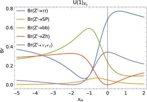
Figure 1: Branching ratios of the $Z^{\prime}$ decay for $g_{X}=0.1,m_{S}=130$ GeV and $m_{Z^{\prime}}=350$ GeV.

II.3 Decay of $P$

If $S$ and $P$ are strongly degenerate so that the mass difference is much smaller than the mass of $Z^{\prime}$, the two body decay of $P$ is kinematically forbidden. Thus, for the main decay mode, $P\rightarrow SZ^{\prime}{}^{*}\rightarrow Sf\bar{f}$, the total decay width ($\Gamma$), or equivalently the inverse of the lifetime ($\tau$),

$$\Gamma=\frac{1}{\tau}=\frac{1}{2p^{0}}\int\overline{|\mathcal{M}(P\rightarrow Sf\bar{f})|^{2}}dQ,$$ (17)

is suppressed by the phase space volume Mohapatra:2023aei . As a result, $P$ is short-lived in cosmology but can be long-lived in collider experiments. The expected travel distance $c\tau$ for $x_{H}=-2$, in other words $U(1)_{R_{3}}$, is shown as the function of its mass $m_{P}$ in Fig. 2. We note that the mass difference,

$$m_{P}^{2}-m_{S}^{2}=2\sqrt{2}Av_{2},$$ (18)

from Eqs. (10) and (11), is always adjustable by suitably choosing the free parameter $A$ such that $c\tau$ becomes about $100$ m, which is ideal for the detection of $P$ decay inside the MATHUSLA detector. Here and hereafter, we have forcused on the $U(1)_{R_{3}}$ case. For $x_{H}\neq-2$, the decay mode of $P\rightarrow SZ^{\prime}{}^{*}\rightarrow S\nu_{\tau}\nu_{\tau}$ exits and becomes the dominant mode for $M_{P}-m_{S}\leq 2m_{\tau}$. In this case, the LPP $P$ provides only invisible decay products.

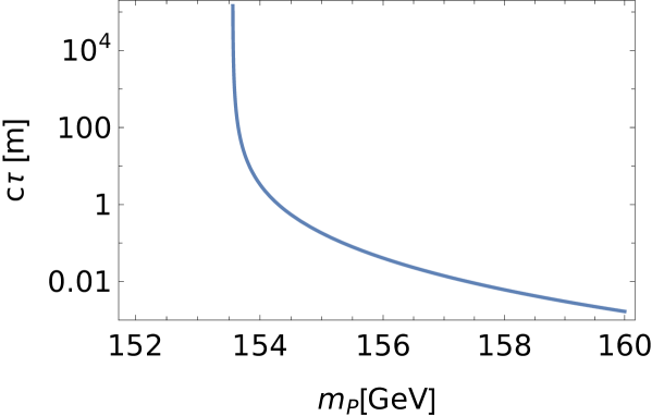
Figure 2: $c\tau$ for $g_{R_{3}}=0.1,m_{S}=150$ GeV and $m_{Z^{\prime}}=350$ GeV. Near the threshold $m_{P}-m_{S}\simeq 2m_{\tau}$ with $m_{\tau}$ being the tau-lepton mass, $c\tau$ is very long.

III Dark matter and LHC constraints

For evaluation of prospect at MATHUSLA in the next section, in this section, we will find a benchmark point which satisfies the thermal DM abundance and the latest LHC constraints. As metioned above, we concentrate on the $U(1)_{R_{3}}$ model. The LLP $P$ in other general $U(1)_{X_{3}}~{}(x_{H}\neq-2)$ may decay into neutrinos which are invisible for the MATHUSLA detector. Thus, the $U(1)_{R_{3}}$ model is the best choice from the viewpoint of the detection with a large decay length of $\mathcal{O}(100)$ m.

III.1 Thermal relic abundance

We estimate the thermal relic abundance of the real scalar DM, $S$, by solving the Boltzmann equation,

$$\frac{dn}{dt}+3Hn=-\langle\sigma_{\mathrm{eff}}v\rangle(n^{2}-n_{\rm EQ}^{2}),$$ (19)

where $H$ and $n_{\rm EQ}$ are the Hubble parameter and the DM number density at thermal equilibrium, respectively KolbTurner . In our model, the main annihilation mode is coannihilation $SP\rightarrow f\bar{f}$ through $s$-channel $Z^{\prime}$ exchange for $m_{Z^{\prime}}>m_{S}$ and the annihilation mode $SS\rightarrow Z^{\prime}Z^{\prime}$ by $u(t)$-channel $P$ exchange for $m_{Z^{\prime}}<m_{S}$ Okada:2019sbb . We use the effective thermal averaged annihilation cross section

$$\langle\sigma_{\mathrm{eff}}v\rangle=\sum_{i,j=S,P}\langle\sigma_{ij}v_{ij}\rangle\frac{n_{i}}{n_{\rm EQ}}\frac{n_{j}}{n_{\rm EQ}},$$ (20)

to include the coannihilation effects properly and $n$ in Eq. (19) should be understood as $n=\sum_{i}n_{i}$ for $i=S,P$ Griest:1990kh ; Edsjo:1997bg . The contours of thermal DM abundance $\Omega h^{2}\simeq 0.1$ Planck:2018vyg (blue curve) and $\mathrm{Br}(Z^{\prime}\rightarrow SP)$ (green curves) for the $U(1)_{R_{3}}$ model are shown in Fig. 3.

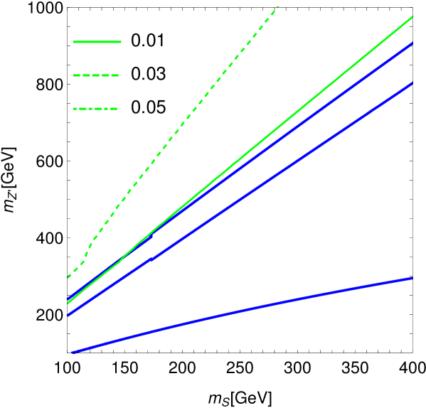
Figure 3: The contour (in blue) along which the observed DM relic abundance $\Omega h^{2}\simeq 0.1$ is reproduced for $g_{R_{3}}=0.1$ and $x_{H}=-2$.

III.2 Benchmark points

To find a viable benchmark point, we also take the $Z^{\prime}$ boson search at the LHC with ditau final state CMS:2024pjt ; ATLAS:2019erb into account. We evaluate the production cross section for the process $pp\rightarrow\tau^{+}\tau^{-}$ given by

$$\sigma(pp\rightarrow Z^{\prime})\mathrm{BR}(Z^{\prime}\rightarrow\tau^{+}\tau^{-}),$$ (21)

where the branching ratio is calculated from Eq. (13). As can be seen in Eq. (14), $\mathrm{BR}(Z^{\prime}\rightarrow\tau^{+}\tau^{-})$ depends on the value of $x_{H}$, and we forcus on $x_{H}=-2$ as stated above.

With the decay rates of $X$ estimated in Sec. II.2, as in Ref. Das:2019fee , since the total $X$ boson decay width is very narrow, we use the narrow width approximation to evaluate the $X$ boson production cross section

$$\sigma(pp\rightarrow X) =2\sum_{q,\bar{q}}\int dx\int dyf_{q}(x,Q)f_{\bar{q}}(x,Q)\hat{\sigma}(\hat{s}),$$ (22)

$$\hat{\sigma}(\hat{s}) =\frac{4\pi^{2}}{3}\frac{\Gamma_{X}(X\rightarrow q\bar{q})}{m_{X}}\delta(\hat{s}-m_{X}^{2}),$$ (23)

where $f_{q}$ and $f_{\bar{q}}$ are the parton distribution function (PDF) for a quark and antiquark ($b$ and $\bar{b}$ in our model), $\hat{s}=xys$ is the invariant mass squared of colliding quarks for the center of mass energy $s$. The factor $2$ in Eq. (22) counts two ways of $q$ coming from which proton out of two colliding protons. Since the most severe bound is from the dilepton channel ($\ell=\tau$), we calculate $\sigma(pp\rightarrow X)\mathrm{Br}(X\rightarrow\tau^{+}\tau^{-})$ and compare it with the CMS results CMS:2024pjt . We employ PDFs of CTEQ6L Pumplin:2002vw with a factorization scale $Q=m_{Z^{\prime}}$ for simplicity.

The resultant production cross section is shown in the second column in Tab. 3. The production cross section is consistent with and smaller than the latest most stringent bound from the CMS CMS:2024pjt at the LHC. We summarize parameters and masses of relevant particles in Tab. 2.

		$x_{H}$	$g_{X_{3}}$	$m_{Z^{\prime}}$	$m_{S}$
$BP_{-2}$		$-2$	$0.1$	$351$ GeV	$150$ GeV

Table 2:

IV Prospect for MATHUSLA

The travel distance $c\tau\simeq 100$ m is the most sensitive range at MATHUSLA  Chou:2016lxi ; Curtin:2017izq ; Curtin:2017bxr . The pair production cross section of such a LLP $\chi$ for its $5\sigma$ discovery can be read as $\sigma_{\chi\chi}>0.3$ fb from Fig. 1 in Ref. Jana:2018rdf . On the other hand, in our scenario, the LLP $P$ is not pair produced but singly produced through $pp\rightarrow Z^{\prime}\rightarrow SP$. Thus, the required production cross section for the LLP $P$ to be discovered at the MATHUSLA would be set to be larger than $0.6$ fb. In Tab. 3, we list the $SP$ production cross section at $13$ TeV LHC and $14$ TeV LHC for our benchmark on Tab. 2 satisfying the DM abundance and the LHC bounds. We find that the MATHUSLA will be able to discover those LLPs because the production cross section $\sigma_{SP}$ is sufficiently larger than $0.6$ fb.

		$\sigma(pp\rightarrow Z^{\prime}\rightarrow\tau\tau)$ (CMS bound on it)		$\sigma_{SP}$ @$13$TeV LHC	$\sigma_{SP}$ @$14$TeV LHC
$BP_{-2}$		$154$ fb ($<203$ fb)		$10.8$ fb	$12.9$ fb

Table 3:

V Summary

We have proposed a simple extension of the SM with an extra $U(1)_{R_{3}}$ gauge interaction with scalar particle of DM candidate with the charge $1$, third generation of SM fermions and third generation of right-handed neutrinos. After the SM singlet $U(1)_{R_{3}}$ breaking scalar with the charge $2$ develops the VEV, the gauge boson acquires the mass, and the tiny mass splitting between real and imaginary component of the charge $1$ scalar appears through the scalar tri-linear interaction. The lighter scalar $S$ is inelastic DM candidate with the heavier state $P$. Due to the mass degeneracy, the slightly heavier state $P$ is long-lived and will be able to be discovered as LLPs.

We have calculated the production cross section of LLP $P$ through the process $pp\rightarrow Z^{\prime}\rightarrow SP$ at the MATHUSLA for a benchmark point which satisfies stringent LHC bounds and thermal DM abundance. The production cross section of benchmark point turns out to be about $10$ fb, which is about an order of magnitude larger than the cross section required by $5\sigma$ discovery as a LLP at the MATHUSLA. Thus, we conclude that the heavier state of inelastic DM in our model can be discovered at the MATHUSLA.

Appendix A The decay rate of $P$

The spin averaged squared amplitude for $P(p)\rightarrow f(q_{1})\bar{f}(q_{2})S(q_{3})$ is given by

$$\overline{|\mathcal{M}|^{2}}$$

$$= \frac{2g_{R_{3}}^{4}}{m_{Z^{\prime}}^{4}\left(-2\left(p\cdot q_{3}\right)+m_{P}^{2}+m_{S}^{2}-m_{Z^{\prime}}^{2}\right)^{2}}\left(-2\left(-m_{P}^{2}+m_{S}^{2}+m_{Z^{\prime}}^{2}\right)^{2}\left(p\cdot q_{1}\right)^{2}\right.$$

$$-2\left(m_{P}^{2}-m_{S}^{2}+m_{Z^{\prime}}^{2}\right)^{2}\left(q_{1}\cdot q_{3}\right)^{2}+4\left(\left(m_{P}^{2}-m_{S}^{2}\right)^{2}-m_{Z^{\prime}}^{4}\right)\left(p\cdot q_{1}\right)\left(q_{1}\cdot q_{3}\right)$$

$$-2\left(-m_{P}^{2}+m_{S}^{2}+m_{Z^{\prime}}^{2}\right)^{2}\left(p\cdot q_{1}\right)\left(p\cdot q_{3}\right)+2\left(m_{P}^{2}-m_{S}^{2}+m_{Z^{\prime}}^{2}\right)^{2}\left(q_{1}\cdot q_{3}\right)\left(p\cdot q_{3}\right)$$

$$\left.+m_{f}^{2}\left(-2\left(\left(m_{P}^{2}-m_{S}^{2}\right)^{2}-m_{Z^{\prime}}^{4}\right)\left(p\cdot q_{3}\right)+m_{Z^{\prime}}^{4}\left(m_{P}^{2}+m_{S}^{2}\right)+\left(m_{P}^{2}-m_{S}^{2}\right)^{2}\left(m_{P}^{2}+m_{S}^{2}-2m_{Z^{\prime}}^{2}\right)\right)\right.$$

$$\left.+\left(p\cdot q_{1}\right)\left(m_{Z^{\prime}}^{4}\left(m_{P}^{2}-3m_{S}^{2}\right)+2m_{Z^{\prime}}^{2}\left(m_{S}^{4}-m_{P}^{4}\right)+\left(m_{P}^{2}-m_{S}^{2}\right)^{2}\left(m_{P}^{2}+m_{S}^{2}\right)\right)\right.$$

$$\left.+\left(q_{1}\cdot q_{3}\right)\left(m_{P}^{4}\left(m_{S}^{2}-2m_{Z^{\prime}}^{2}\right)+m_{P}^{2}\left(m_{S}^{4}+3m_{Z^{\prime}}^{4}\right)-m_{P}^{6}-\left(m_{S}^{3}-m_{S}m_{Z^{\prime}}^{2}\right)^{2}\right)\right).$$ (24)

The integration of phase space volume is reduced to

$$dQ= \frac{d^{3}q_{1}}{(2\pi)^{3}2q_{1}^{0}}\frac{d^{3}q_{2}}{(2\pi)^{3}2q_{2}^{0}}\frac{d^{3}q_{3}}{(2\pi)^{3}2q_{3}^{0}}(2\pi)^{4}\delta^{(4)}\left(p-q_{1}-q_{2}-q_{3}\right)$$

$$= \frac{1}{(2\pi)^{5}}\frac{d^{3}q_{1}}{2q_{1}^{0}}\frac{d^{3}q_{3}}{2q_{3}^{0}}\delta\left((m_{P}-q_{1}^{0}-q_{3}^{0})^{2}-(|\mathbf{q}_{1}|^{2}+|\mathbf{q}_{3}|^{2})-2|\mathbf{q}_{1}||\mathbf{q}_{3}|\cos\theta_{13}-m_{f}^{2}\right)$$

$$= \frac{1}{8(2\pi)^{5}}dq_{1}^{0}dq_{3}^{0}d\Omega_{1}d\varphi_{13}d\cos\theta_{13}\delta\left(\frac{(m_{P}-q_{1}^{0}-q_{3}^{0})^{2}-|\mathbf{q}_{1}|^{2}-|\mathbf{q}_{3}|^{2}-m_{f}^{2}}{2|\mathbf{q}_{1}||\mathbf{q}_{3}|}-\cos\theta_{13}\right).$$ (25)

Then, the integration range of energy turns out to be

$$q_{3}^{\mathrm{min}}(q_{1}^{0})<q_{3}^{0}<q_{3}^{\mathrm{max}}(q_{1}^{0}),$$ (26)

with

$$q_{3}^{\mathrm{min}}(q_{1}^{0})=\frac{\left(m_{P}-q_{1}^{0}\right)\left(m_{P}^{2}-2m_{P}q_{1}^{0}+m_{S}^{2}\right)-\sqrt{\left(\left(q_{1}^{0}\right)^{2}-m_{f}^{2}\right)\left(\left(m_{P}^{2}-2m_{P}q_{1}^{0}-m_{S}^{2}\right)^{2}-4m_{f}^{2}m_{S}^{2}\right)}}{2\left(m_{f}^{2}+m_{P}\left(m_{P}-2q_{1}^{0}\right)\right)},$$ (27)

$$q_{3}^{\mathrm{max}}(q_{1}^{0})=\frac{\left(m_{P}-q_{1}^{0}\right)\left(m_{P}^{2}-2m_{P}q_{1}^{0}+m_{S}^{2}\right)+\sqrt{\left(\left(q_{1}^{0}\right)^{2}-m_{f}^{2}\right)\left(\left(m_{P}^{2}-2m_{P}q_{1}^{0}-m_{S}^{2}\right)^{2}-4m_{f}^{2}m_{S}^{2}\right)}}{2\left(m_{f}^{2}+m_{P}\left(m_{P}-2q_{1}^{0}\right)\right)},$$ (28)

and

$$m_{f}<q_{1}^{0}<\frac{m_{P}^{2}-m_{S}^{2}-2m_{f}m_{S}}{2m_{P}}.$$ (29)

By integrating the differential decay rate

$$d\Gamma=\frac{1}{2p^{0}}\overline{|\mathcal{M}|^{2}}dQ=\frac{1}{8(2\pi)^{3}m_{P}}\left[\overline{|\mathcal{M}|^{2}}\delta\left(\cdots-\cos\theta_{13}\right)d\cos\theta_{13}\right]dq_{1}^{0}dq_{3}^{0},$$ (30)

for the range (26) and (29), we obtain the travel distance shown in Fig. 2.

References

- (1) G. Aad et al. [ATLAS], JHEP 2306, 158 (2023).
- (2) H. Abreu et al. [FASER], Phys. Lett. B 848, 138378 (2024).
- (3) A. Ariga et al. [FASER], Phys. Rev. D 99, no.9, 095011 (2019).
- (4) J. P. Chou, D. Curtin and H. J. Lubatti, Phys. Lett. B 767, 29-36 (2017).
- (5) P. S. Bhupal Dev, R. N. Mohapatra and Y. Zhang, Phys. Rev. D 95, no.11, 115001 (2017).
- (6) J. A. Evans, Phys. Rev. D 97, no.5, 055046 (2018).
- (7) J. C. Helo, M. Hirsch and Z. S. Wang, JHEP 07, 056 (2018).
- (8) F. F. Deppisch, W. Liu and M. Mitra, JHEP 08, 181 (2018).
- (9) S. Jana, N. Okada and D. Raut, Phys. Rev. D 98, no.3, 035023 (2018).
- (10) M. Bauer, M. Heiles, M. Neubert and A. Thamm, Eur. Phys. J. C 79, no.1, 74 (2019).
- (11) D. Curtin, K. R. Dienes and B. Thomas, Phys. Rev. D 98, no.11, 115005 (2018).
- (12) A. Berlin and F. Kling, Phys. Rev. D 99, no.1, 015021 (2019).
- (13) D. Dercks, J. De Vries, H. K. Dreiner and Z. S. Wang, Phys. Rev. D 99, no.5, 055039 (2019).
- (14) F. Deppisch, S. Kulkarni and W. Liu, Phys. Rev. D 100, no.3, 035005 (2019).
- (15) J. M. No, P. Tunney and B. Zaldivar, JHEP 03, 022 (2020).
- (16) Z. S. Wang and K. Wang, Phys. Rev. D 101, no.7, 075046 (2020).
- (17) K. Jodłowski, F. Kling, L. Roszkowski and S. Trojanowski, Phys. Rev. D 101, no.9, 095020 (2020).
- (18) P. D. Bolton, F. F. Deppisch and P. S. Bhupal Dev, JHEP 03, 170 (2020).
- (19) M. Hirsch and Z. S. Wang, Phys. Rev. D 101, no.5, 055034 (2020).
- (20) S. Jana, N. Okada and D. Raut, Eur. Phys. J. C 82, no.10, 927 (2022).
- (21) J. Gehrlein and S. Ipek, JHEP 05, 020 (2021).
- (22) C. Sen, P. Bandyopadhyay, S. Dutta and A. KT, Eur. Phys. J. C 82, no.3, 230 (2022).
- (23) J. Guo, Y. He, J. Liu and X. P. Wang, JHEP 04, 024 (2022).
- (24) B. Bhattacherjee, S. Matsumoto and R. Sengupta, Phys. Rev. D 106, no.9, 095018 (2022).
- (25) M. Du, R. Fang, Z. Liu and V. Q. Tran, Phys. Rev. D 105, no.5, 055012 (2022).
- (26) A. Kamada and T. Kuwahara, JHEP 03, 176 (2022).
- (27) E. Bertuzzo, A. Scaffidi and M. Taoso, JHEP 08, 100 (2022).
- (28) W. Liu, J. Li, J. Li and H. Sun, Phys. Rev. D 106, no.1, 015019 (2022).
- (29) P. Bandyopadhyay, E. J. Chun and C. Sen, JHEP 02, 103 (2023).
- (30) Y. n. Mao, K. Wang and Z. S. Wang, Phys. Rev. D 108, no.9, 095025 (2023).
- (31) K. Jodłowski, Phys. Rev. D 108, no.11, 11 (2023).
- (32) P. J. Fitzpatrick, Y. Hochberg, E. Kuflik, R. Ovadia and Y. Soreq, Phys. Rev. D 108, no.7, 075003 (2023).
- (33) D. Curtin and J. S. Grewal, Phys. Rev. D 109, no.7, 075017 (2024).
- (34) A. Batz, T. Cohen, D. Curtin, C. Gemmell and G. D. Kribs, JHEP 04, 070 (2024).
- (35) F. F. Deppisch, S. Kulkarni and W. Liu, [arXiv:2311.01719 [hep-ph]].
- (36) N. Bernal, K. Deka and M. Losada, Phys. Rev. D 110, no.5, 055011 (2024).
- (37) F. Bishara, F. Sala and K. Schmidt-Hoberg, [arXiv:2401.12278 [hep-ph]].
- (38) W. Liu, L. Wang and Y. Zhang, Phys. Rev. D 110, no.1, 015016 (2024).
- (39) J. de Vries, H. K. Dreiner, J. Groot, J. Y. Günther and Z. S. Wang, [arXiv:2406.15091 [hep-ph]].
- (40) S. Liebersbach, P. Sandick, A. Shiferaw and Y. Zhao, [arXiv:2408.07756 [hep-ph]].
- (41) E. Aprile et al. [XENON], Phys. Rev. Lett. 131, no.4, 041003 (2023).
- (42) A. Cuoco, M. Krämer and M. Korsmeier, Phys. Rev. Lett. 118, no.19, 191102 (2017).
- (43) A. McDaniel, M. Ajello, C. M. Karwin, M. Di Mauro, A. Drlica-Wagner and M. A. Sánchez-Conde, Phys. Rev. D 109, no.6, 063024 (2024).
- (44) N. Okada and O. Seto, Phys. Rev. D 101, no.2, 023522 (2020).
- (45) L. J. Hall, T. Moroi and H. Murayama, Phys. Lett. B 424, 305 (1998).
- (46) D. Tucker-Smith and N. Weiner, Phys. Rev. D 64, 043502 (2001).
- (47) K. Griest and D. Seckel, Phys. Rev. D 43, 3191 (1991).
- (48) J. Edsjo and P. Gondolo, Phys. Rev. D 56, 1879 (1997).
- (49) E. W. Kolb and M. S. Turner, The Early Universe, Addison-Wesley (1990).
- (50) J. C. Pati and A. Salam, Phys. Rev. D 8, 1240-1251 (1973).
- (51) A. Davidson, Phys. Rev. D 20, 776 (1979).
- (52) R. N. Mohapatra and R. E. Marshak, Phys. Rev. Lett. 44, 1316 (1980) [Erratum-ibid. 44, 1643 (1980)].
- (53) R. E. Marshak and R. N. Mohapatra, Phys. Lett. B 91, 222 (1980).
- (54) M. Carena, A. Daleo, B. A. Dobrescu and T. M. P. Tait, Phys. Rev. D 70, 093009 (2004).
- (55) S. Amrith, J. M. Butterworth, F. F. Deppisch, W. Liu, A. Varma and D. Yallup, JHEP 1905, 154 (2019).
- (56) A. Das, P. S. B. Dev and N. Okada, Phys. Lett. B 799, 135052 (2019).
- (57) K. S. Babu, A. Friedland, P. A. N. Machado and I. Mocioiu, JHEP 1712, 096 (2017).
- (58) R. Alonso, P. Cox, C. Han and T. T. Yanagida, Phys. Lett. B 774, 643 (2017).
- (59) L. Bian, S. M. Choi, Y. J. Kang and H. M. Lee, Phys. Rev. D 96, no. 7, 075038 (2017).
- (60) P. Cox, C. Han and T. T. Yanagida, JCAP 1801, no. 01, 029 (2018).
- (61) P. del Amo Sanchez et al. [BaBar Collaboration], Phys. Rev. Lett. 104, 191801 (2010).
- (62) D. A. Faroughy, A. Greljo and J. F. Kamenik, Phys. Lett. B 764, 126 (2017).
- (63) M. Aaboud et al. [ATLAS Collaboration], JHEP 1801, 055 (2018).
- (64) E. J. Chun, A. Das, J. Kim and J. Kim, JHEP 1902, 093 (2019).
- (65) F. Elahi and A. Martin, Phys. Rev. D 100, no. 3, 035016 (2019).
- (66) T. Appelquist, B. A. Dobrescu and A. R. Hopper, Phys. Rev. D 68 035012 (2003).
- (67) S. Oda, N. Okada and D. s. Takahashi, Phys. Rev. D 92, no. 1, 015026 (2015).
- (68) A. Das, S. Oda, N. Okada and D. s. Takahashi, Phys. Rev. D 93 no.11, 115038 (2016).
- (69) S. Jung, H. Murayama, A. Pierce and J. D. Wells, Phys. Rev. D 81, 015004 (2010).
- (70) N. Okada and O. Seto, Phys. Rev. D 98, no. 6, 063532 (2018).
- (71) W. Chao, W. F. Cui, H. K. Guo and J. Shu, Chin. Phys. C 44, no.12, 123102 (2020)
- (72) G. Jungman, M. Kamionkowski and K. Griest, Phys. Rept. 267, 195 (1996).
- (73) R. N. Mohapatra and N. Okada, Phys. Rev. D 107, no.9, 095023 (2023).
- (74) N. Aghanim et al. [Planck], Astron. Astrophys. 641, A6 (2020) [erratum: Astron. Astrophys. 652, C4 (2021)].
- (75) [CMS], CMS-PAS-EXO-21-016.
- (76) G. Aad et al. [ATLAS], Phys. Lett. B 796, 68-87 (2019).
- (77) J. Pumplin, D. R. Stump, J. Huston, H. L. Lai, P. M. Nadolsky and W. K. Tung, JHEP 07, 012 (2002).
- (78) D. Curtin and M. E. Peskin, Phys. Rev. D 97, no.1, 015006 (2018).
- (79) D. Curtin, K. Deshpande, O. Fischer and J. Zurita, JHEP 07, 024 (2018).