Qubit coupled with an effective negative-absolute-temperature bath in off-resonant collision model

Abstract

Quantum collision model provides a promising tool for investigating system-bath dynamics. Most of the studies on quantum collision models work in the resonant regime. In quantum dynamics, the off-resonant interaction often brings in exciting effects. It is thereby attractive to investigate quantum collision models in the off-resonant regime. On the other hand, a bath with a negative absolute temperature is anticipated to be instrumental in developing thermal devices. The design of an effective bath with negative absolute temperature coupled to a qubit is significant for developing such thermal devices. We establish an effective negative-absolute-temperature bath coupled to a qubit with a quantum collision model in a far-off-resonant regime. We conduct a detailed and systematic investigation on the off-resonant collision model. There is an additional constraint on the collision duration resulting from the far-off resonant collision. The dynamics of the collision model in the far-off-resonant regime are different from the one beyond the far-off-resonant regime. Numerical simulations confirm the validity of the proposed approach.

I introduction

Quantum collision model is a powerful and effective tool for investigating the dynamics of the system-bath scheme Lorenzo et al. (2015a, b); Pezzutto et al. (2016); Strasberg et al. (2017); Cusumano et al. (2018); Seah et al. (2019); Rodrigues et al. (2019); Barra (2019); Molitor and Landi (2020); Taranto et al. (2020); Campbell and Vacchini (2021); Ciccarello et al. (2022); Zhang et al. (2023a, b). It first appeared in 1963 Rau (1963) and has gained growing use in the last few years. In quantum collision model, the bath is represented by an extensive collection of subunits (ancillas). The open system is coupled to the bath by the system-ancilla short collisions, i.e., short unitary interactions. The collisions are performed through a pairwise sequence. In most quantum collision models, the system resonantly interacts with the ancillas. In investigating the dynamics of a quantum system, it is common to encounter a situation in which quantum objects off-resonantly interact with each other. These off-resonant interactions often bring fresh effects James and Jerke (2007) compared to the resonant interaction. For example, a two-level system far-off-resonantly driven by an external weak Laser would gain slight shifts of its levels, known as the A. C. Stark shift. An atom with an appropriate structure interacting with light can induce a large nonlinear effect when light off-resonantly drives the specific level transition Schmidt and Imamoglu (1996); Hartmann et al. (2006). In quantum technology, a widely used approach to couple the decoupled levels of interest is to introduce the intermediate auxiliary levels working in the off-resonant regime, as shown in the examples (in the vast number of instances) in Refs. Hartmann et al. (2007); Zheng and Guo (2000); Campbell and Hudson (2020); Zhang et al. (2024). Therefore, it is reasonable that quantum collision model in the off-resonant regime, i.e., the system off-resonantly colliding with the ancillas, may bring in fresh effects compared to the resonant case. A systematic investigation of the quantum collision model in the off-resonant regime would inject more vitality into the field of quantum collision model.

In recent years, negative absolute temperature has caused intensive attention. Onsager originally conceived the physical idea of the negative absolute temperature in the statistical investigation of the point vortices Onsager (1949), which has been demonstrated in recent experiments with the two-dimensional quantum superfluid Johnstone et al. (2019); Gauthier et al. (2019). Subsequently, Purcell and Pound observed the negative absolute temperatures in the nuclear spin systems with LiF crystal Purcell and Pound (1951). Ramsey theoretically investigated the thermodynamic and statistical mechanical implications of such negative absolute temperatures Ramsey (1956). While there is some confusion regarding the equilibrium of negative absolute temperature related to the definition of entropy Dunkel and Hilbert (2014); Calabrese and Porporato (2019), negative absolute temperatures are now widely accepted in the scientific community and appear consistent with experimental observations Frenkel and Warren (2015); Buonsante et al. (2016); Puglisi et al. (2017); Cerino et al. (2015); Abraham and Penrose (2017); Baldovin et al. (2021); Onorato et al. (2022); Baudin et al. (2023); Muniz et al. (2023). The negative absolute temperature bath is expected to develop thermal devices such as Carnot engines Geusic et al. (1967); Landsberg (1977); Nakagomi (1980); Dunning-Davies (1976); Dunning‐Davies (1978); Landsberg et al. (1980); Xi and Quan (2017); de Assis et al. (2019); Nettersheim et al. (2022); Maity and De (2023); Maity and Ghoshal (2024); de Sousa et al. (2024) and refrigerators Damas et al. (2023), in which the devices involved in the negative absolute temperature bath would perform better than their traditional counterparts based on positive temperatures. In this context, for most proposals, the negative temperature bath was assumed to exist already or was realized by external driving or work. Notably, the authors in Ref. Bera et al. (2024) proposed an approach to realize a synthetic negative temperature bath coupled to a three-level atom. The temperature of the synthetic bath could be an arbitrary value in the range from $-\infty$ to $+\infty$. It opens up an issue on how to realize a negative temperature bath coupled to a qubit, a unit of quantum information widely used in constructing quantum thermal devices.

In this paper, we propose to realize an effective negative temperature bath coupled to a qubit in the context of quantum collision model in the off-resonant regime. The qubit is effectively realized by adiabatically eliminating the highest level of a $\Lambda$-type qutrit when the ancillas of the effective bath far-off resonantly collide with the qutrit. Under certain conditions, based on the dynamics of the proposed collision scheme, a Gorini-Kossakowski-Sudarshan-Lindblad master equation, which represents the dynamics of a qubit coupled to an effective bath with adjustable temperature, is found by performing appropriate approximations. The validity of the master equation is confirmed by numerical simulations, which is necessary to ensure the rigor of this work because we have not found any precedent to handle quantum collision models in our way. We find that an additional constraint on the collision duration is impressed since the lower bound of the coarse-graining time stems from the rapid oscillation dynamics of the far-off-resonant collisions. Beyond the far-off-resonant-collision case, one can not realize the effective qubit-bath coupling because it is difficult to neglect the dynamics of the highest level of the qutrit. In this case, the dynamics are similar to those outlined in Ref. Bera et al. (2024).

II Collision Model

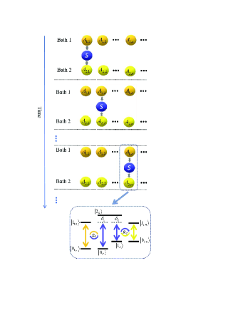
Figure 1: Collision model: the system S composed of a three-level qutrit undergoes sequence successive collisions with the ancilla qubits in bath 1 and bath 2.

The collision model under consideration is sketched in Fig. 1. The open system S consists of a $\Lambda$-type qutrit. The three levels of S are labeled by $\left|0_{S}\right\rangle$, $\left|1_{S}\right\rangle$, and $\left|2_{S}\right\rangle$, with the corresponding level frequencies denoted by $\omega_{S,0}$, $\omega_{S,1}$, and $\omega_{S,2}$, respectively. There are two baths, either of which contains many identical ancillas, i.e., noninteracting qubits, coupled to the open system via a sequence of system-ancilla collisions. The $n$-th ($n=1,2,3...$) ancilla of bath $m$ ($m=1,2$) is labeled by $A_{m,n}$. The upper and lower levels of $A_{m,n}$ are denoted by $\left|1_{A_{m,n}}\right\rangle$ and $\left|0_{A_{m,n}}\right\rangle$, respectively. The frequency corresponding to the upper (lower) level of bath $m^{\prime}$s identical qubits is labeled by $\omega_{A_{m,1}}$ ($\omega_{A_{m,0}}$). We focus on the collisional memoryless model. Each ancilla collides with the system S only once. The $n$-th collision step is realized by the short interaction of S with $A_{1,n}$ and $A_{2,n}$. The system level transitions $\left|0_{S}\right\rangle\leftrightarrow\left|2_{S}\right\rangle$ and $\left|1_{S}\right\rangle\leftrightarrow\left|2_{S}\right\rangle$ are coupled to the ancilla level transitions $\left|1_{A_{1,n}}\right\rangle\leftrightarrow\left|0_{A_{1,n}}\right\rangle$ and $\left|1_{A_{2,n}}\right\rangle\leftrightarrow\left|0_{A_{2,n}}\right\rangle$, respectively. In the interaction picture, the Hamiltonian representing the $n$-th collision step reads

$$H_{n}=g_{1}\sigma_{A_{1,n}}^{10}\sigma_{S}^{02}e^{-i\delta_{1}t}+g_{2}\sigma_{A_{2,n}}^{10}\sigma_{S}^{12}e^{-i\delta_{2}t}+h.c.,$$ (1)

where $\sigma_{M}^{kk^{\prime}}=\left|k_{M}\right\rangle\left\langle k_{M}^{\prime}\right|$ is $M$’s level transition and population operators with $M\in\{A_{1,n},A_{2,n},S\}$. The interaction strength between $A_{m,n}$ and the system is denoted by $g_{m}$, which remains unchanged with the collision step number $n$. The detunings $\delta_{1}$ and $\delta_{2}$ are represented by $\delta_{1}=\omega_{S,20}-\omega_{A_{1}}$ and $\delta_{2}=\omega_{S,21}-\omega_{A_{2}}$, respectively, as shown in Fig. 1. Here $\omega_{S,kk^{\prime}}=\omega_{S,k}-\omega_{S,k^{\prime}}$ denotes the system level transition frequency between the levels $\left|k_{S}\right\rangle$ and $\left|k_{S}\right\rangle$, and $\omega_{A_{m}}=\omega_{A_{m,1}}-\omega_{A_{m,0}}$ is the level transition frequency of the qubit in bath $m$. We have set the reduced Plank constant $\hbar$ as a unit, i.e., $\hbar=1$. The first (second) term in Hamiltonian (1) represents the off-resonant interaction between $A_{1,n}$ ($A_{2,n}$) and S when $\delta_{1}$ ($\delta_{2}$) is nonzero. In the far-off-resonant case, i.e., the large-detuning case represented as $\delta_{m}\gg g_{m}$, one can perform the standard adiabatic elimination James and Jerke (2007) and obtain the effective Hamiltonian as

$$H_{eff,n} = -\alpha_{11}\sigma_{A_{1,n}}^{11}\sigma_{S}^{00}-\alpha_{22}\sigma_{A_{2,n}}^{11}\sigma_{S}^{11}$$ (2)

$$-\alpha_{12}\sigma_{A_{1,n}}^{01}\sigma_{A_{2,n}}^{10}\sigma_{S}^{10}e^{i(\delta_{1}-\delta_{2})t}+h.c.,$$

where $\alpha_{mn}=\frac{g_{m}g_{n}}{2}(\frac{1}{\delta_{m}}+\frac{1}{\delta_{n}})$. The vital condition $\left|\delta_{1}-\delta_{2}\right|\ll\alpha_{12}$ should be satisfied so that the dynamics governed by the second line of the effective Hamiltonian (2) play a significant role and are not ignored. The effective Hamiltonian eliminates the system’s highest level $\left|2_{S}\right\rangle$, which is referred to as a virtual level in the subsequent analysis. Either of the terms in the first line of the effective Hamiltonian can be understood by a sequence of two virtual procedures. Taking the first term as an example, in the first virtual procedure, $A_{1,n}$ makes the transition $\left|1_{A_{1,n}}\right\rangle\rightarrow\left|0_{A_{1,n}}\right\rangle$, meanwhile, S jumps from the level $\left|0_{S}\right\rangle$ to the virtual level. In the second virtual procedure, $A_{1,n}$ flips back to level $\left|1_{A_{1,n}}\right\rangle$; meanwhile, S flips back to level $\left|0_{S}\right\rangle$. The second line can be understood from the fact that S jumps between the levels $\left|0_{S}\right\rangle$ and $\left|1_{S}\right\rangle$ via the virtual level; meanwhile, $A_{1,n}$ and $A_{2,n}$ accomplish their corresponding level transitions.

The terms in the first line of the effective Hamiltonian result in slight shifts of the corresponding levels. To understand this level-shift effect, one can consult the analysis represented by Ref. Neumeier et al. (2013), in which similar interactions are investigated. The effective Hamiltonian implies that the system S is an effective qubit with the levels $\left|0_{S}\right\rangle$ and $\left|1_{S}\right\rangle$. The two ancillas cooperatively drive the common effective-qubit-level transition in each collision step. Here, we take the condition $\delta_{1}=\delta_{2}=\delta$ so that the energy absorbed (or released) by the effective-qubit-level transition equals the energy released (or absorbed) by the cooperative ancilla-level transitions.

The legitimacy of the adiabatic elimination on the level $\left|2_{S}\right\rangle$ is confirmed in Fig. 2, which numerically simulates the dynamics governed by the original Hamiltonian (1) and effective Hamiltonian (2) in the far-off-resonant case. The symbols $p_{k}^{orig}$ and $p_{k}^{eff}$ denote the populations of $\left|k_{S}\right\rangle$ obtained by solving the original Hamiltonian and effective Hamiltonian, respectively. In Fig. 2 (a), the evolution of $p_{0}^{eff}$ ($p_{1}^{eff}$) agrees well with the evolution of $p_{0}^{orig}$ ($p_{1}^{orig}$). The population of the level $\left|2_{S}\right\rangle$ governed by the original Hamiltonian is always near zero. As shown in Fig. 2 (b), the evolutions of the populations governed by the original Hamiltonian show extremely slight but rapid oscillations against time. One of the critical approximations performed in the adiabatic elimination is that the effective Hamiltonian has considered the coarse-grained (or time-averaged) dynamics of the original Hamiltonian. The slight oscillations can not be visually observed in Fig. 2 (a) because the evolution time is much larger than the coarse-graining time, and the maximum values of the populations are much larger than the oscillation amplitudes.

Figure 2: Numerical simulation of the populations against the time governed by Hamiltonian (1) and (2). The initial state is set as $\left|1_{A_{1,n}},0_{A_{2,n}},0_{S}\right\rangle$. (a) shows the evolutions of the populations from $\alpha_{11}t=0$ to $\alpha_{11}t=5$, and (b) shows the evolutions from $\alpha_{11}t=0$ to $\alpha_{11}t=0.006$. In (b), in order to observe the slight oscillations of evolutions governed by Hamiltonian (1), the populations of the state $\left|1_{S}\right\rangle$ is represented as the insert panel because the difference between the population of $\left|0_{S}\right\rangle$ and the population of $\left|1_{S}\right\rangle$ is much larger than the amplitudes of the oscillations. The green, red, and blue solid lines denote $p_{0}^{orig}$, $p_{1}^{orig}$, and $p_{2}^{orig}$, respectively. In (a), $p_{0}^{orig}$ and $p_{1}^{orig}$ are represented by green and red hollow circles, respectively. While, in (b), $p_{0}^{orig}$ and $p_{1}^{orig}$ are represented by green and red dotted lines, respectively. The parameters are $g_{2}=g_{1}$ and $\delta=50g_{1}$.

III Continuous-Time Master Equation

It will be convenient to bring in the rotating frame with respect to the term $-\alpha_{11}\sigma_{A_{1,n}}^{11}\sigma_{S}^{00}-\alpha_{22}\sigma_{A_{2,n}}^{11}\sigma_{S}^{11}$. In this rotating frame, the effective Hamiltonian turns out to be

$$V_{n}=-\alpha\sigma_{A_{1,n}}^{01}\sigma_{A_{2,n}}^{10}\sigma_{S}^{10}+h.c.,$$ (3)

where we have taken $g_{1}=g_{2}=g$ and hence $\alpha_{11}=\alpha_{22}=\alpha_{12}=\alpha$. The collision durations in all the steps are assumed equal and denoted by $\tau$. The unitary evolution operator $U_{n}=e^{-iV_{n}\tau}$ represents the evolution of the n-th collision step.

Before the n-th collision step, the system and the n-th qubits of the two baths are considered in the state $\sigma_{n-1}=\rho_{n-1}\otimes\eta_{A_{1,n}}\otimes\eta_{A_{2,n}}$, where the density operators $\rho_{n-1}$, $\eta_{A_{1,n}}$, and $\eta_{A_{2,n}}$ represent the states of S, $A_{1,n}$, and $A_{2,n}$, respectively. Initially, the qubits in bath 1 and 2 are in the Gibbs thermal state with inverse temperatures $\beta_{1}$ and $\beta_{2}$, respectively, i.e.,

$$\eta_{A_{m,n}}=\frac{\sigma_{A_{m,n}}^{11}+e^{\omega_{A_{m}}\beta_{m}}\sigma_{A_{m,n}}^{00}}{e^{\omega_{A_{m}}\beta_{m}}+1}.$$

By performing the approximation up to the second-order of $\tau$, one can obtain

$$\Delta\rho_{n} = Tr_{A_{1},A_{2}}(U\sigma_{n-1}U^{\dagger}-\sigma_{n-1})$$ (4)

$$\sim Tr_{A_{1},A_{2}}(-i\tau[V_{n},\sigma_{n-1}]+\tau^{2}(V_{n}\sigma_{n-1}V_{n}$$

$$-\frac{1}{2}[\sigma_{n-1},V_{n}^{2}]_{+}),$$

where the anti-commutator $[\cdot,\cdot]_{+}$ satisfies $[A,B]_{+}=AB+BA$. Eqn. (4) denotes the stroboscopic representation of the system dynamics with the discrete-time variables $t_{n}=n\tau$ ($n=1,2,3...$). When the collision duration $\tau$ is much smaller than the evolution time scale, one can consider the continuous-time limit, i.e. $\frac{\Delta\rho_{n}}{\tau}\rightarrow\frac{d\rho}{dt}$, and obtain a continuous-time master equation as

$$\frac{d\rho}{dt} = \Gamma e^{\omega_{S,10}\beta_{S}}(\sigma_{S}^{01}\rho\sigma_{S}^{10}-\frac{1}{2}[\rho,\sigma_{S}^{11}]_{+})$$ (5)

$$+\Gamma(\sigma_{S}^{10}\rho\sigma_{S}^{01}-\frac{1}{2}[\rho,\sigma_{S}^{00}]_{+}),$$

where $\beta_{s}=\frac{\omega_{A_{1}}\beta_{1}-\omega_{A_{2}}\beta_{2}}{\omega_{A_{1}}-\omega_{A_{2}}}$ and $\Gamma=\frac{R^{2}g^{2}\tau}{(1+e^{\omega_{A_{1}}\beta_{1}})(1+e^{-\omega_{A_{2}}\beta_{2}})}$ with $R$ the ratio of coupling strength to the detuning, i.e., $R=\frac{g}{\delta}$. $R$ is dimensionless when the dimension of $g$ is the same as that of $\delta$. The steady-state solution of Eqn. (5) can be easily found as

$$\rho_{ss}=\frac{\sigma_{S}^{11}}{1+e^{\omega_{S,10}\beta_{S}}}+\frac{e^{\omega_{S,10}\beta_{S}}\sigma_{S}^{00}}{1+e^{\omega_{S,10}\beta_{S}}},$$ (6)

representing that the effective qubit is the thermal state with the inverse temperature $\beta_{s}$. It is as if an effective bath synthesized by integrating bath 1 and bath 2 is coupled to the effective qubit. The inverse temperature $\beta_{s}$ of the effective bath can be tuned by the level-transition frequency and initial Gibbs state of the ancillas. The far-off-resonant collision model outlines an approach that couples a qubit to an effective bath with an arbitrary temperature, including a negative temperature.

IV Collision Duration and Coarse-Graining Time

The short but finite collision duration is a coarse-graining time, and the collision step is a coarse-grained procedure. We recall that the rapid slight oscillation dynamics governed by Hamiltonian (1) has been coarse-grained by the effective Hamiltonian (2) under the large-detuning condition, which naturally arises a constraint on the collision duration. The constraint is that the collision duration should be significantly longer than the time scale of the rapid-slight-oscillation period. We proceed to demonstrate the validity of the continuous-time master equation (5) numerically under this constraint.

One should return to the original Hamiltonian (1) to numerically simulate the collided system’s accurate dynamics. It will be convenient to look for a new rotating frame in which the Hamiltonian is time-independent. In the rotating frame with respect to $-\delta\sigma_{S}^{22}$, the time-independent Hamiltonian is found as

$$H_{n}^{\prime}=\delta\sigma_{S}^{22}+g\sigma_{A_{1,n}}^{10}\sigma_{S}^{02}+g\sigma_{A_{2,n}}^{10}\sigma_{S}^{12}+h.c.$$ (7)

the subscript $\prime$ in the operator $O^{\prime}$ implies that the operator $O$ is represented in the new rotating frame. After n-th collision step, the reduced density operator for the system is

$$\rho_{n}^{\prime}=Tr_{A_{1},A_{2}}\sum_{m,m^{\prime}}e^{-i(\epsilon_{m}-\epsilon_{m^{\prime}})\tau}\left\langle m\right|\sigma_{n-1}^{\prime}\left|m^{\prime}\right\rangle\left|m\right\rangle\left\langle m^{\prime}\right|\text{,}$$ (8)

where $\left|m\right\rangle$ and $\left|m^{\prime}\right\rangle$ are the eigenvectors of the time-independent Hamiltonian $H_{n}^{\prime}$, with $\epsilon_{m}$ and $\epsilon_{m^{\prime}}$ the corresponding eigenvalues. Alternatively, $\rho_{n}^{\prime}$ can also be found by

$$\rho_{n}^{\prime}=Tr_{A_{1},A_{2}}\sigma^{\prime}(\tau),$$ (9)

with $\sigma^{\prime}(\tau)$ the solution of Liouville equation $\dot{\sigma}^{\prime}(t)=-i[H_{n}^{\prime},\sigma^{\prime}(t)]$ at the time point $t=\tau$ by considering the initial condition $\sigma^{\prime}(0)=\sigma_{n-1}^{\prime}$. Then, the numerical simulation of the system state after each collision step could be obtained by the numerical iterations according to Eqn. (8) or (9). The numerical simulation would fit the system’s accurate dynamics with high precision because no approximation has been performed to obtain the analytical form of Eqns. (8) and (9).

The numerical simulations in Fig. 3 compare the accurate dynamics of the collided system with the dynamics of the continuous-time master equation (5) for different collision durations. The system’s accurate dynamics are numerically simulated based on Eqn. (9), in which the numeral solution of Liouville equation is derived by the 4-order Runger-Kutta method. Let us discuss three situations.

In situation (a), the collision duration is too small to satisfy the constraint. The evolution described by Eqn. (5) significantly differs from the system’s accurate evolution, as confirmed in Fig. 3 (a) when $\alpha\tau=0.01$. In the accurate evolution, the collided system can jump to the level $\left|2_{S}\right\rangle$ with a non-negligible probability. It can be understood from the fact that, although the coarse-grained dynamics of the level $\left|2_{S}\right\rangle$ is negligible in the large detuning case, the level transition between $\left|0_{S}\right\rangle$ and $\left|2_{S}\right\rangle$ plays the predominant role when the evolution duration is in (or smaller than) the time scale of the rapid-slight-oscillation period, as shown in Fig. 2 (b). In this situation, the coarse-graining on the dynamics does not work well, and the level $\left|2_{S}\right\rangle$ is not negligible. The qutrit can not be considered an effective qubit, and hence, the continuous-time master equation (5) is not valid.

In situation (b), the collision duration is significantly longer than the time scale of the rapid-slight-oscillation period and much shorter than the evolution time scale. As shown in Fig. 3 (b), the population evolution governed by Eqn. (5) agrees with the system’s accurate evolution reasonably well. Although the temperatures of the baths are set significantly large, it is difficult to obtain a noticeable population of level $\left|2_{S}\right\rangle$. Therefore, the continuous-time master equation (5) can represent the system dynamics well.

In situation (c), the collision duration is not short enough compared to the evolution time scale, so the system dynamics are not effectively time-continuous. It is challenging to represent the system dynamics by continuous-time master equations.

V Beyond the far-off-resonant case

According to the dynamics governed by the original Hamiltonian (1), a continuous-time master equation quite different from the master equation (5) can be obtained. In the rotating frame introduced in section IV, the unitary evolution operator is defined as $U_{n}^{\prime}=e^{-iH_{n}^{\prime}\tau}$. For the short collision duration, one can make the approximation up to the second-order of the $\tau$ and find a continuous-time master equation as

$$\frac{d\rho^{\prime}}{dt} = i\delta[\rho,\sigma_{S}^{22}]+\tau\delta^{2}(\sigma_{S}^{22}\rho\sigma_{S}^{22}-\frac{1}{2}[\rho,\sigma_{S}^{22}]_{+})$$ (10)

$$+\gamma_{1}e^{\omega_{A_{1}}\beta_{1}}(\sigma_{S}^{02}\rho\sigma_{S}^{20}-\frac{1}{2}[\rho,\sigma_{S}^{22}]_{+})$$

$$+\gamma_{1}(\sigma_{S}^{20}\rho\sigma_{S}^{02}-\frac{1}{2}[\rho,\sigma_{S}^{00}]_{+})$$

$$+\gamma_{2}e^{\omega_{A_{2}}\beta_{2}}(\sigma_{S}^{12}\rho\sigma_{S}^{21}-\frac{1}{2}[\rho,\sigma_{S}^{22}]_{+})$$

$$+\gamma_{2}(\sigma_{S}^{21}\rho\sigma_{S}^{12}-\frac{1}{2}[\rho,\sigma_{S}^{11}]_{+})$$

with $\gamma_{m}=\frac{g^{2}\tau}{1+e^{\omega_{A_{m}}\beta_{m}}}$. It represents that the qutrit is coupled to bath 1 and bath 2, i.e., the level transition $\left|0_{S}\right\rangle\leftrightarrow\left|2_{S}\right\rangle$ is coupled to the bath 1, and the transition $\left|1_{S}\right\rangle\leftrightarrow\left|2_{S}\right\rangle$ is coupled to the bath 2. In particular, when $\delta=0$, it turns out to be the case represented in Ref. Bera et al. (2024).

Although the continuous-time master equations (5) and (10) represent different dynamics, they do not conflict because they work under different conditions. To represent this in detail, we emphasize that the approximations up to the second order of $\tau$ are essential to obtain both Eqns. (5) and (10). For Eqn. (5), the approximation holds when the high-order terms on $\alpha\tau$ can be well ignored, which can be understood by substituting the expression of $V_{n}$ into the approximate transformation $U_{n}\sim I-iV_{n}\tau-\frac{(V_{n}\tau)^{2}}{2}$. Distinctly, for Eqn. (10), the approximation holds when the high-order terms on $\delta\tau$ and $g\tau$ can be well ignored, which can be understood by substituting the expression of $H_{n}^{\prime}$ into $U_{n}^{\prime}\sim I-iH_{n}^{\prime}\tau-\frac{(H_{n}^{\prime}\tau)^{2}}{2}$. As a consequence, for Eqn. (10), it would work well if the detuning $\delta$ is not extremely large. In contrast, Eqn. (5), stemming from the effective Hamiltonian (2), works well under the large-detuning case. Consequently, the larger the detuning $\delta$ is, the better the performance of Eqn. (5) is. Besides, one can verify that, by the parameters in Fig. 3, it is challenging to perform the approximations up to the second-order of $\tau$ to obtain Eqn. (10) when the collision duration is significantly longer than the time scale of the rapid-slight-oscillation period.

VI conclusions

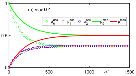
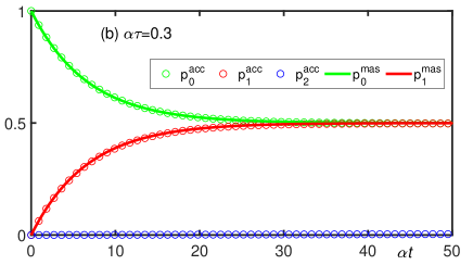
Figure 3: Numerical simulations of the collided-system-level-population evolution governed by the original Hamiltonian (1) and the master equation (5). The system initial state is $|0_{S}\rangle$, and the parameters are $\Delta=200g,\omega_{A_{1}}\beta_{1}=\omega_{A_{2}}\beta_{2}=10^{-4}$. We take $\alpha\tau=0.01$ in (a) and $\alpha\tau=0.3$ in (b). The original-Hamiltonian-governing populations of levels $|0_{S}\rangle$, $|1_{S}\rangle$, and $|2_{S}\rangle$ are labeled by $p_{0}^{acc}$, $p_{1}^{acc}$, and $p_{2}^{acc}$, and plotted by the green, red and blue hollow circles, respectively. The subscript ”acc” denotes that it is the simulation of the system’s accurate dynamics. The master-equation-governing populations of levels $|0_{S}\rangle$ and $|1_{S}\rangle$ are labeled by $p_{0}^{mas}$ and $p_{1}^{mas}$, and plotted by the green and red solid lines, respectively. The blue hollow circles in (a) overlap with the red ones.

In conclusion, we propose a quantum collision model in which an open system composed of a qutrit off-resonantly collides with the ancillas of two baths. The qutrit interacts with two ancillas from two baths in each collision step. In the far-off-resonant case, according to a legal adiabatic elimination on the highest level of the qutrit, we show that the qutrit-ancilla interaction is effectively considered as the two ancillas commonly driving the level transition of a qubit. A master equation, which implies that our scheme is considered a qubit coupled to an effective bath, is found in the continuous-time limit via coarse-graining. It shows that the temperature of the effective bath can be an arbitrary negative real number. The validity of the approach is confirmed by numerically comparing the system’s accurate dynamics to the qubit dynamics represented by the master equation. Because the far-off-resonant interaction results in rapid oscillation dynamics, the collision duration should be significantly longer than the rapid oscillation period to ensure that each collision process is coarse-grained. It differs from the quantum collision model working in a resonant regime as there are no rapid oscillation dynamics. Beyond the far-off-resonant case, the system dynamics can be represented by a master equation implying a qutrit coupled to two independent baths, where the highest level of the qutrit can not be legally adiabatically eliminated, and the qutrit is not regarded as an effective qubit. The work outlines an approach to couple a qubit with an effective negative temperature based on quantum collision model. It systematically investigates the quantum collision model in the off-resonant regime. It also implies the approaches to realize an effective negative temperature coupled to a qubit based on conventional thermal baths. For example, a qutrit is coupled to two conventional thermal baths, where the frequencies of the baths are filtered so that they are far different from the corresponding level transition frequencies of the qutrit. Alternatively, it implies a theoretically reasonable but experimentally challenging approach in which two conventional thermal baths are coupled to a common qubit.

References

- Lorenzo et al. (2015a) S. Lorenzo, R. McCloskey, F. Ciccarello, M. Paternostro, and G. M. Palma, Phys. Rev. Lett. 115, 120403 (2015a).
- Lorenzo et al. (2015b) S. Lorenzo, A. Farace, F. Ciccarello, G. M. Palma, and V. Giovannetti, Phys. Rev. A 91, 022121 (2015b).
- Pezzutto et al. (2016) M. Pezzutto, M. Paternostro, and Y. Omar, New Journal of Physics 18, 123018 (2016).
- Strasberg et al. (2017) P. Strasberg, G. Schaller, T. Brandes, and M. Esposito, Phys. Rev. X 7, 021003 (2017).
- Cusumano et al. (2018) S. Cusumano, V. Cavina, M. Keck, A. De Pasquale, and V. Giovannetti, Phys. Rev. A 98, 032119 (2018).
- Seah et al. (2019) S. Seah, S. Nimmrichter, D. Grimmer, J. P. Santos, V. Scarani, and G. T. Landi, Phys. Rev. Lett. 123, 180602 (2019).
- Rodrigues et al. (2019) F. L. S. Rodrigues, G. De Chiara, M. Paternostro, and G. T. Landi, Phys. Rev. Lett. 123, 140601 (2019).
- Barra (2019) F. Barra, Phys. Rev. Lett. 122, 210601 (2019).
- Molitor and Landi (2020) O. A. D. Molitor and G. T. Landi, Phys. Rev. A 102, 042217 (2020).
- Taranto et al. (2020) P. Taranto, F. Bakhshinezhad, P. Schüttelkopf, F. Clivaz, and M. Huber, Phys. Rev. Appl. 14, 054005 (2020).
- Campbell and Vacchini (2021) S. Campbell and B. Vacchini, Europhysics Letters 133, 60001 (2021).
- Ciccarello et al. (2022) F. Ciccarello, S. Lorenzo, V. Giovannetti, and G. M. Palma, Physics Reports 954, 1 (2022).
- Zhang et al. (2023a) Q. Zhang, Z.-X. Man, Y.-J. Zhang, W.-B. Yan, and Y.-J. Xia, Phys. Rev. A 107, 042202 (2023a).
- Zhang et al. (2023b) Q. Zhang, Y.-J. Xia, and Z.-X. Man, Phys. Rev. A 108, 062211 (2023b).
- Rau (1963) J. Rau, Phys. Rev. 129, 1880 (1963).
- James and Jerke (2007) D. F. James and J. Jerke, Canadian Journal of Physics 85, 625 (2007).
- Schmidt and Imamoglu (1996) H. Schmidt and A. Imamoglu, Optics Letters 21, 1936 (1996).
- Hartmann et al. (2006) M. J. Hartmann, F. G. S. L. Brandão, and M. B. Plenio, Nature Physics 2, 849 (2006).
- Hartmann et al. (2007) M. J. Hartmann, F. G. S. L. Brandão, and M. B. Plenio, Phys. Rev. Lett. 99, 160501 (2007).
- Zheng and Guo (2000) S.-B. Zheng and G.-C. Guo, Phys. Rev. Lett. 85, 2392 (2000).
- Campbell and Hudson (2020) W. C. Campbell and E. R. Hudson, Phys. Rev. Lett. 125, 120501 (2020).
- Zhang et al. (2024) F.-Y. Zhang, S.-W. He, T. Liu, Q.-C. Wu, and C.-P. Yang, Phys. Rev. A 109, 022442 (2024).
- Onsager (1949) L. Onsager, Il Nuovo Cimento (1943-1954) 6, 279 (1949).
- Johnstone et al. (2019) S. P. Johnstone, A. J. Groszek, P. T. Starkey, C. J. Billington, T. P. Simula, and K. Helmerson, Science 364, 1267 (2019).
- Gauthier et al. (2019) G. Gauthier, M. T. Reeves, X. Yu, A. S. Bradley, M. A. Baker, T. A. Bell, H. Rubinsztein-Dunlop, M. J. Davis, and T. W. Neely, Science 364, 1264 (2019).
- Purcell and Pound (1951) E. M. Purcell and R. V. Pound, Phys. Rev. 81, 279 (1951).
- Ramsey (1956) N. F. Ramsey, Phys. Rev. 103, 20 (1956).
- Dunkel and Hilbert (2014) J. Dunkel and S. Hilbert, Nature Phys 10, 67 (2014).
- Calabrese and Porporato (2019) S. Calabrese and A. Porporato, Physics Letters A 383, 2153 (2019).
- Frenkel and Warren (2015) D. Frenkel and P. B. Warren, American Journal of Physics 83, 163 (2015).
- Buonsante et al. (2016) P. Buonsante, R. Franzosi, and A. Smerzi, Annals of Physics 375, 414 (2016).
- Puglisi et al. (2017) A. Puglisi, A. Sarracino, and A. Vulpiani, Physics Reports 709-710, 1 (2017).
- Cerino et al. (2015) L. Cerino, A. Puglisi, and A. Vulpiani, Journal of Statistical Mechanics: Theory and Experiment 2015, 12002 (2015).
- Abraham and Penrose (2017) E. Abraham and O. Penrose, Phys. Rev. E 95, 012125 (2017).
- Baldovin et al. (2021) M. Baldovin, S. Iubini, R. Livi, and A. Vulpiani, Physics Reports 923, 1 (2021).
- Onorato et al. (2022) M. Onorato, G. Dematteis, D. Proment, A. Pezzi, M. Ballarin, and L. Rondoni, Phys. Rev. E 105, 014206 (2022).
- Baudin et al. (2023) K. Baudin, J. Garnier, A. Fusaro, N. Berti, C. Michel, K. Krupa, G. Millot, and A. Picozzi, Phys. Rev. Lett. 130, 063801 (2023).
- Muniz et al. (2023) A. L. M. Muniz, F. O. Wu, P. S. Jung, M. Khajavikhan, D. N. Christodoulides, and U. Peschel, Science 379, 1019 (2023).
- Geusic et al. (1967) J. E. Geusic, E. O. Schulz-DuBios, and H. E. D. Scovil, Phys. Rev. 156, 343 (1967).
- Landsberg (1977) P. T. Landsberg, Journal of Physics A: Mathematical and General 10, 1773 (1977).
- Nakagomi (1980) T. Nakagomi, Journal of Physics A: Mathematical and General 13, 291 (1980).
- Dunning-Davies (1976) J. Dunning-Davies, Journal of Physics A: Mathematical and General 9, 605 (1976).
- Dunning‐Davies (1978) J. Dunning‐Davies, American Journal of Physics 46, 583 (1978).
- Landsberg et al. (1980) P. T. Landsberg, R. J. Tykodi, and A. M. Tremblay, Journal of Physics A: Mathematical and General 13, 1063 (1980).
- Xi and Quan (2017) J.-Y. Xi and H.-T. Quan, Communications in Theoretical Physics 68, 347 (2017).
- de Assis et al. (2019) R. J. de Assis, T. M. de Mendonça, C. J. Villas-Boas, A. M. de Souza, R. S. Sarthour, I. S. Oliveira, and N. G. de Almeida, Phys. Rev. Lett. 122, 240602 (2019).
- Nettersheim et al. (2022) J. Nettersheim, S. Burgardt, Q. Bouton, D. Adam, E. Lutz, and A. Widera, PRX Quantum 3, 040334 (2022).
- Maity and De (2023) A. Maity and A. S. De, arXiv 2304.10420 (2023).
- Maity and Ghoshal (2024) A. Maity and A. Ghoshal, Phys. Rev. A 109, 022207 (2024).
- de Sousa et al. (2024) A. F. de Sousa, G. G. Damas, and N. G. de Almeida, arXiv 2404.02385 (2024).
- Damas et al. (2023) G. G. Damas, R. J. de Assis, and N. G. de Almeida, Physics Letters A 482, 129038 (2023).
- Bera et al. (2024) M. L. Bera, T. Pandit, K. Chatterjee, V. Singh, M. Lewenstein, U. Bhattacharya, and M. N. Bera, Phys. Rev. Res. 6, 013318 (2024).
- Neumeier et al. (2013) L. Neumeier, M. Leib, and M. J. Hartmann, Phys. Rev. Lett. 111, 063601 (2013).