Master stability curves for traveling waves

Abstract

Computing the spectrum and stability of traveling waves in spatially discrete systems quickly becomes unfeasible with increasing system size. We present a framework for effectively determining the spectrum and stability of traveling waves in discrete systems with symmetries (such as rings and lattices) by computing master stability curves. We show that wave destabilization and multi-stability between waves can be determined from the position and curvature of master stability curves independently of the number of constituents. To illustrate our framework, we compute and analyze master stability curves of traveling waves (that take the form of pulse trains) in diffusively coupled rings of FitzHugh-Nagumo oscillators.

Since the pioneering works of Fermi, Pasta, Ulam, and Tsingou [1, 2], traveling wave phenomena in discrete spatially-extended systems —such as spikes, pulses, solitons, fronts, and breathers— have attracted attention in various application areas, including neuroscience [3, 4, 5], nonlinear optics [6, 7, 8], chemical reactions [9], crystal dislocations [10, 11, 12], Ising-like phase transitions [13, 14], conservation laws [15], coupled oscillators [16, 17], traffic jams [18], etc. Such traveling waves in discrete spatially-extended systems, henceforth discrete traveling waves (DTWs), have received a lot of attention both analytically [19, 20] and numerically [21]. A related phenomenon (not studied here) is discrete (traveling) breathers [22] where the spatial wave profile varies in time (in addition to propagating through the system). Additionally, DTWs have also been observed in discretizations of continuous spatially extended systems, such as discrete-nonlinear-Schrödinger or Frenkel-Kantorova-type models [23, 24, 25]. Notably, sufficiently slow waves in continuous systems can exhibit failure of propagation in the discrete case [26].

Characterizing the stability of DTWs has remained a challenging problem often addressed under particular approximations [12]. Rigorous results can be obtained in special cases or under additional symmetry requirements. For instance, the stability of DTWs in rings with weak coupling has been addressed [27] and, through a similar reduction method [28], the stability of rotating wave solution in delay-coupled feed-forward ring networks [29] and feed-forward discrete torus of Stuard-Landau oscillators [30] have been investigated. The stability of standing waves (zero wave speed) has also been studied [31].

Considering the importance of DTWs in applications, there is a fundamental need for a unifying theory describing the spectral properties of such waves in analogy to the master stability function approach developed by Pecora and Carroll [32] for synchronization in networks (when all nodes behave dynamically the same). The dimension of the master stability function developed by Pecora and Carroll is independent of the network size, and it serves as a roadmap for the stability of synchronization for any network.

In this letter, we outline such a master stability theory for DTWs on networks and coupled systems of ordinary differential equations that are invariant under cyclic index shift ($\mathbb{Z}_{N}$-equivariant) [33]. Notable examples of $\mathbb{Z}_{N}$-equivariant coupled systems are systems of $N$ identical nodes coupled in a (possibly nonlocal) ring, spatial discretizations of partial differential equations with periodic boundary conditions, and systems with higher-order coupling topologies [34] invariant under cyclic index shift, as well as —by little extension— multi-chromatic networks, discrete tori, and systems with higher spatial embedding order (see End Matter for details).

Our method relies on a suitable transformation that recasts the higher dimensional Floquet spectral problem as a delay differential equation, possibly of mixed type, the master stability equation. Using the derived equation, we introduce a numerical scheme based on the continuation of a suitable two-point boundary problem to assess the stability of such waves by computing master stability curves (MSCs).

Setup.

To set the stage, we consider the $N$-dimensional network with $d$-dimensional internal dynamics given by

$$x^{\prime}_{n}= F(x_{n})+\!\!\!\!\sum_{1\leq|m|\leq r}\!\!\!\!H_{m}(x_{n},x_{n+m}),\quad x_{n}(t)\in\mathbb{R}^{d}.$$ (1)

Here, $x_{n}$, $n=1,2,\ldots,N$, represents a node in the network, and $x_{n}^{\prime}$ denotes its first derivative with respect to time $t$. The function $F$ defines the uncoupled dynamics at each node $x_{n}$. Each node $x_{n}$ is coupled to nodes $x_{n+m}$ (using the convention $x_{j}=x_{j+N}$ for $j\in\mathbb{Z}$) through the functions $H_{m}$, $1\leq|m|\leq r$, where $r$ represents the coupling radius of the network. A comprehensive treatment of systems featuring higher-order interactions (see, e.g., [34]) can be found in the End Matter. Notice that system (1) is equivariant under cyclic permutation $x_{n}\mapsto x_{n+1}$ (mod $N$); and hence supports DTWs [33].

Our results pertain to the stability of DTWs of the form

$$x_{n}(t)=y(t-n\tau),\quad y(t)\in\mathbb{R}^{d},$$ (2)

where $y$ is the $T$-periodic profile of the wave propagating with constant wave speed $c=1/\tau$ (one unit of space per unit of time). Since we are dealing with finite networks, there is a consistency relation $k=\tau/T$ that defines a wave number $k$ ($1/k$ being the wavelength).

Figure 1(a)-(b) shows two examples of such waves with wave number $k=0.05$ and constant wave speed $c\approx 0.6764$ in system (8) with (a) $N=20$ and (b) $N=100$ nodes. In both cases, the wave profile is the same, which can be understood as follows: The DTWs corresponding to the profile $y$ (here with wave number $k=1/20$) can be supported in a network of size $N=K/k$, where $K\in\mathbb{N}$, by concatenating $K$ copies of the profile and thus changing neither wave number nor period. As such, Fig. 1(a) shows the minimal network size realization of a DTW with profile $y$ and $k=1/20$. The stability of these waves is determined by the sign of the real part of their Floquet exponents (FEs); particularly, a FE $\lambda\in\mathbb{C}$ together with its bundle $u=(u_{1},...,u_{N})$ can be computed as solutions of the $Nd$-dimensional Floquet periodic boundary value problem (FP)

$$u^{\prime}_{n}(t)= \left(A(t-n\tau)-\lambda I\right)u_{n}(t)$$ (3)

$$+\!\!\!\!\sum_{1\leq|m|\leq r}\!\!\!\!B_{m}(t-n\tau)u_{n+m}(t),$$

$$u_{n}(t)= u_{n}(t+T),$$

where $u_{n}(t)\in\mathbb{C}^{d}$, with $T$-periodic coefficient functions

$$A(t)= DF(y(t))+\!\!\!\!\sum_{1\leq|m|\leq r}\!\!\!\!D_{1}H_{m}(y(t),y(t-m\tau)),$$

$$B_{m}(t)= D_{2}H_{m}(y(t),y(t-m\tau)).$$

Here, $D_{1}H_{m}$ and $D_{2}H_{m}$ denote the Jacobians of $H_{m}$ with respect to its first and second arguments, respectively. It is the case that, if a $\lambda$ is a FE, then $\lambda+2\pi i/T$ is also a FE. Particularly, the collection of all FEs with imaginary parts inside the interval $[-2\pi i/T,2\pi i/T)$ is called the Floquet spectrum with size equal to $Nd$ (counting multiplicity). Particularly, if Re$(\lambda)<0$ for all the FEs except for the trivial exponent $\lambda=0$ (Goldstone mode), then the DTW (2) is (orbitally) stable.

There are multiple existing ways to numerically obtain the Floquet spectrum, ranging from solving the FP explicitly to finding the eigenvalues of the monodromy matrix [35]. In any case, the computations become infeasible or inaccurate as the system size $N$ or the period $T$ becomes larger.

Our proposed method accounts for these issues as exemplified in Fig. 1(c)-(d). Here, the $N$ largest FEs (in real part) of the waves shown in panels (a) for $N=20$ (black circles) and (b) for $N=100$ (blue dots) reveal that both waves are orbitally stable. Moreover, the FEs appear to delineate a curve. This suggests an accumulation of FEs of DTWs with constant wave number $k=0.05$ as $N\to\infty$, a phenomenon observed previously for DTWs in a feed-forward ring of duffing oscillators [17]. Indeed, we find such a limiting object (shown in cyan), and it takes the form of a curve, which we refer to as the master stability curve (MSC). The MSC can be used to determine the stability and spectrum of a given wave for arbitrarily large $N$. In this letter, we show how to compute MSCs using numerical methods for delay differential equations [36].

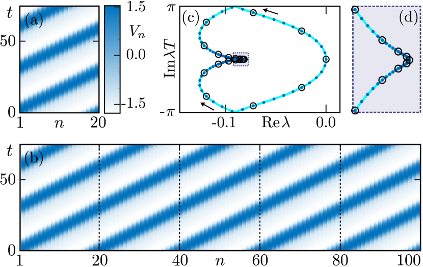
Figure 1: Master stability curve (MSC) in system (8) of $N$ dissipatively-coupled FitzHugh-Nagumo oscillators $x_{n}=(V_{n},W_{n})$. Here, $V_{n}(t)$ and $W_{n}(t)\in\mathbb{R}$. Panel (a)–(b): Space-time plots of DTWs with wave number $k=1/20$. Panel (a): $N=20$. Panel (b): $N=100$. Panel (c): Floquet exponents with Re$(\lambda)\geq-0.3$ of wave in (a) (black circles), of wave in (b) (blue dots), and MSC (cyan). Panel (d): enlargement of the shaded region in (c).

Master stability equation.

We now outline the method for computing MSCs by means of continuation. First, we bring (3) into a more convenient form. By using the component-wise time-shift transformation $v_{n}(t)=u_{n}(t+n\tau),$ FP (3) can be recast as

$$v^{\prime}_{n}(t)= \left(A(t)-\lambda I\right)v_{n}(t)+\!\!\!\!\sum_{1\leq|m|\leq r}\!\!\!\!B_{m}(t)v_{n+m}(t-m\tau),$$ (4)

$$v_{n}(t)= v_{n}(t+T).$$

System (4) can be diagonalized under the discrete Fourier transform

$$\hat{v}_{l}=\sum_{n=1}^{N}v_{n}e^{-in\phi_{l}},\quad v_{l}(t)\in\mathbb{R}^{d}$$

where $l=1,\ldots,N$ and $\phi_{l}=2\pi l/N$, such that for each FE $\lambda$, every $\hat{v}_{l}$ is a solution of the $d$-dimensional periodic boundary problem

$$\hat{v}_{l}^{\prime}(t)= \left(A(t)-\lambda I\right)\hat{v}_{l}(t)+\!\!\!\!\sum_{1\leq|m|\leq r}\!\!\!\!e^{-im\phi_{l}}B_{m}(t)\hat{v}_{l}(t-m\tau),$$ (5)

$$\hat{v}_{l}(t)= ~{}\hat{v}_{l}(t+T).$$

Notice that the $\hat{v}_{l}$ are decoupled and can be solved independently of each other, as opposed to the $v_{n}$, and that (5) is independent of the network size $N$. Hence, we define

$$\hat{\zeta}^{\prime}(t)= \left(A(t)-\lambda I\right)\hat{\zeta}(t)+\!\!\!\!\sum_{1\leq|m|\leq r}\!\!\!\!e^{-im\phi}B_{m}(t)\hat{\zeta}(t-m\tau),$$ (6)

$$\hat{\zeta}(t)= ~{}\hat{\zeta}(t+T),$$

where $\zeta(t)\in\mathbb{R}^{d}$ and $\phi\in[0,2\pi)$, as the master stability equation.

Fixing the norm and angle of $\zeta$ (see End Matter for details), a variation in the parameter $\phi$ defines a one-parameter family of solutions of (6) and, in particular, curves in $\lambda$-space, the MSCs, where all Floquet exponents for a given $k$ must lie on independently of $N$. This can be observed in Fig. 1 where we compare spectra of DTWs with identical wave profiles in a minimal network of $N=20$ nodes (a) and $N=100$ nodes (b). This is where the power of our approach unfolds: Instead of computing the spectra for each case separately, the MSCs capture the spectra of all network realizations of the wave profile $y$. Indeed, whenever $\phi$ is a $N$-th root of unity, then the associated $\lambda$ is a Floquet Exponent of (3). We remark that there might exist more than one MSC; the exact number of MSCs needs to be assessed on a case-by-case basis. Our numerics suggest that the number of MSCs tends to be small, close to $d$. One way to understand this is through the embedding of the wave profile in a minimal network and computing its spectrum directly. Note that only the relevant MSC (closest to the imaginary axis) is shown in Fig. 1, where $d=2$; indeed, there exists one more curve to the left in this particular case which is not shown.

We remark that if one is interested in reconstructing the bundle $u$, one can do so. Indeed, the $n$-th component $u_{n}$ of the corresponding Floquet bundle corresponding to $\lambda$ can be reconstructed by the inverse transformation

$$u_{n}(t)=v_{n}(t-n\tau)=\frac{1}{N}\sum_{l=1}^{N}\hat{v}_{l}(t-n\tau)e^{in\phi_{l}}.$$

However, in practice we observe that for a given $\lambda$ almost all $\hat{v}_{l}$ are identically zero. Indeed, for $\lambda=0$ it is easy to show that $\hat{v}_{l}=0$ for all $l\neq 0$ and the corresponding bundle satisfies $u_{n}(t)=\hat{v}_{0}(t-n\tau)$ (after normalization). This particular property also allows us to initialize the continuation procedure of an MSC using the bundle of the Goldstone mode, as was done in Fig. 1. See End Matter for more detail on the numerical implementation and the number of MSCs obtainable.

Applications of the master stability framework.

Below, we illustrate how the master stability framework allows studying the stability of wave profiles independently of a specific embedding into a given network of size $N$. It is then immediately interesting to see how the MSC changes for different wave profiles. To that aim, we introduce the profile equation corresponding to Eq. (1) in a coordinate frame co-moving with wave profile $y$, i.e.

$$y^{\prime}(t)=F(y(t))+\!\!\!\!\sum_{1\leq|m|\leq r}\!\!\!\!H_{m}(y(t-m\tau)),$$ (7)

which can be readily obtained by imposing (2) on system (1). Notice that $\tau$ can be considered a continuous parameter in Eq. (7). This allows us to apply continuation techniques to Eq. (7) to study how profile and period change as a one-dimensional solution family when $\tau$ is varied. Since the consistency relationship must be satisfied, this will imply a variation of $k$ according to $k=\tau/T$. When $k=p/q\in\mathbb{Q}$, the corresponding profile can be embedded in a suitable network of size $N=Kq$, for any $K\in\mathbb{N}$, by concatenating $Kp$ wave profiles and sampling with time window $p\tau$. In what follows, we present examples for $p=1$ to keep the presentation simple. Below, we show how simultaneous numerical continuation of (6) and (7) can be used to explore (A) wave destabilization and (B) the presence of stable bound multi-pulse by keeping track of the position of the MSC with respect to the imaginary axis.

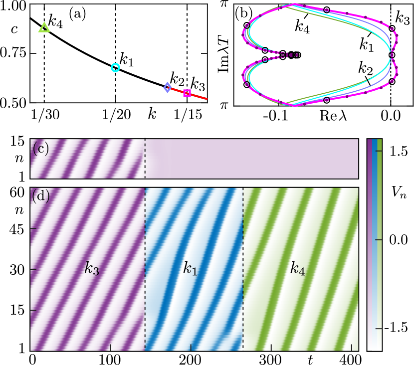
Figure 2: Wave destabilization in system (8) of $N$ dissipatively-coupled FitzHugh-Nagumo oscillators $x_{n}=(V_{n},W_{n})$. Panel (a): Numerical continuation of wave profile shown in Fig. 1 parameterized by wave number $k$. The color of the curve represents the curvature of the MSC at $\lambda=0$; red (black) represents positive (negative) curvature. Panel (b): MSCs of waves at values $k_{1}$ (cyan circle), $k_{2}$ (mauve diamond), $k_{3}$ (magenta square), and $k_{4}$ (green triangle) shown in (a). Also shown are the FE of the wave profile with wave number $k=k_{4}$ for embedding dimension $N=15$ (black circles) and $N=60$ (purple dots). Panels(c)–(d): Long-term dynamics of system (8) starting at unstable wave profile at $k_{3}$ for $N=15$ (c) and $N=60$ (d).

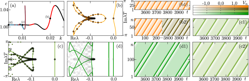
Figure 3: Multi-stability and bound multi-pulses in system (8) of $N$ dissipatively-coupled FitzHugh-Nagumo oscillators $x_{n}=(V_{n},W_{n})$. Panel (a): Numerical continuation of the wave profile shown in Fig. 1 (main profile), and of the bound two-pulse wave profile (secondary profile). Colors represent the curvature of the MSCs close to $\lambda=0$; red (black) represents positive (negative) curvature for the main profile, while dark red (blue) represents positive and negative curvature for the secondary profile. Panel (b): Floquet spectrum when $N=50$ (black circles) and $N=100$ (brown dots), together with MSCs (orange curves) of the main profile at $k=1/50$. Panel (c): Floquet spectrum when $N=100$ (black circles) and $N=200$ (green dots), together with MSCs (light green curves) of the main profile at $k=1/100$. Panel (d): Floquet spectrum (computed with same numerical tolerances as in (b) and (d)) when $N=200$ (gray circles) together with MSCs (dark green curve) of the secondary profile at $k=1/200$. Panels (b1)–(c1): Long-term dynamics of the main profile at points indicated in panel (a) for different embedding dimensions $N$. Panel (d1): Long-term dynamics of the secondary profile as indicated in panel (a) in a network with $N=200$ nodes.

(A) Wave destabilization. Starting with the DTWs shown in Fig. 1, we increase the wave number from $k=k_{1}=1/20$ to $k=k_{3}=1/15$, see Fig. 2(a), and notice a qualitative change of the MSC of the underlying wave profile as shown in Fig. 2(b). Approximately at $k=k_{2}\approx 0.0617$, the MSC displays a change of curvature (from negative to positive) around $\lambda=0$, causing a small segment of the curve to extend into the positive half-plane. The wave profiles for which the MSC has positive curvature at $\lambda=0$ (to the right of $k_{2}$) are colored red in panel (a). The change in curvature is well pronounced for $k=k_{3}$ as exhibited by the magenta curve in panel (b). Also plotted is the spectrum of the corresponding wave profile in a ring of $N=15$ (black circles) and $N=60$ (purple dots), which are both unstable. In the network with fewer nodes, this causes the wave to die out after some transient which is largely determined by the distance of the initial condition used for simulation from the exact unstable wave profile. In the larger network, we observe another phenomenon, which is the multi-stability of DTWs typically accompanied by such modulational-type instabilities. Starting from the unstable profile, we continue from a wave profile with wave number $k_{3}$ to a wave profile with wave number $k_{1}$ by losing a wave crest, before losing another wave crest and settling onto a stable wave profile with wave number $k_{4}=1/30$. Both wave profiles with wave numbers $k_{1}$ and $k_{4}$ are stable, but it appears that the transient has missed the basin of stability of the DTW at $k=k_{1}.$ Notice that this instability allows, in principle, for a scenario in which the wave profile is stable in sufficiently small systems but unstable in systems that are large beyond some finite threshold.

(B) Wave localization and bound two-pulses. Continuing the wave profile shown in Fig. 1 to smaller wave numbers $k$, we observe an oscillatory limiting behavior towards the asymptotic wave speed $c\approx 1.0049$ as we approach $k=0$, see Fig. 3(a). At the same time, the minimal embedding dimension of the profile grows beyond bound, the wave profile localizes in a small number of nodes (a pulse) and its period tends to infinity. We remark that this oscillatory limiting behavior can be attributed to the presence of a homoclinic bifurcation, presumably of Shilnikov-type, in the profile equation at $k=0$, which gives rise to a large degree of multi-stability and the existence of multi-pulses [37]. Another mechanism for the bifurcation of bound multi-pulses from a single pulse in delay differential equations has been studied in [38]. In what follows, we briefly illustrate how the presence of this object manifests in system (8) for $k=0.02,0.01$ and $k=0.05$ and minimal embedding dimension $N=50,100$ and $200$ by showing the existence of stable bound two-pulses for sufficiently small $k$. The results are contained in Fig. 3.

Figure 3(b) shows part of the Floquet spectrum (with largest real parts) of wave profiles at $k=1/50$ together with the corresponding MSC. Notice that the MSC shown has split into two curves as compared to Fig. 1(c) (counting both segments on the left as one curve as they can be continuously parameterized by $\phi$). As part of this transition (details not shown), the curvature of the rightmost MSC has changed from negative to positive locally at $\lambda=0$, and thus, the corresponding DTWs is unstable for sufficiently large embedding dimension $N$. Indeed, for $\phi$ equal to a $50$-th root of unity, $\lambda=0$ in the right-most curve; this implies that the DTW is stable in the network with $N=50$ nodes. However, embedding the same wave profile in a network with $N=100,$ we observe that the corresponding DTW is unstable with a FE $\lambda=\lambda_{0}$ of the form Re$(\lambda_{0})>0,$ Im$(\lambda_{0}T)=i\pi$ whenever $\phi$ and is an odd $100$-th root of unity. This is evidenced by the spectrum in Fig. 3(a) (black circles and orange dots) and direct simulations starting near the wave profile, see Fig. 3(b1)–(b2).

Direct simulation starting near the wave profile with two equidistant pulses, we observe a DTW with non-equidistant pulses (a bound two-pulse). Interestingly, this DTW cannot correspond to the wave profile at $k=1/100$ in panel (a), which is orbitally stable when $N=100$ as can be seen from its spectrum (panel (c)) and by direct simulation (panel (c1)). Rather, the emergence of the bound two-pulse profile observed in panel (b2) can be attributed to the occurrence of a period-doubling bifurcation in the master stability equation when $\lambda_{0}$ crosses the imaginary axis as $k$ is decreased. Indeed, we can use the two-pulse solution obtained in panel (b2) to reconstruct a wave profile corresponding to the secondary curve of bound two-pulse wave profiles in panel (a) (dark red and blue). Furthermore, we observe that the bound two-pulse wave profile approaches a limit as $k$ tends to zero; however, both profiles look different as they near it. To illustrate this, we compare direct simulations in a $N=200$ network when simulating near the original wave profile with $k=1/100$ (panel (c2)) and the bound two-pulse wave profile with $k=1/200$ (panel (d1)). For the bound two-pulse wave profile, the DTW is stable in its minimal network embedding, as evidenced by the spectrum shown in panel (d) and its simulation. On the other hand, the original wave profile is unstable in the $N=200$ network, where its largest unstable FE is close to zero in the real part. Indeed, the MSC in panel (c) attached to $\lambda=0$ has become flat; this suggests a scaling of the real parts of FEs $\lambda$, namely Re$(\lambda)=\mathcal{O}(k)$ on the curve, as $k=1/(cT)\to 0$ for finite values of $c$. This can result in long transients where the solution stays close to the profile, as shown in panel (c2).

Panels (c) and (d) again emphasize the importance of our approach for DTW on large networks. Although the computation of the Floquet spectrum with classical methods begins to fail, we know that all FEs must, in truth, lie on an MSC computed with our framework.

Summary and Outlook.

The spectrum of traveling waves on finite networks (DTWs) with index-shift invariance is determined by the master stability equation and master stability curves (MSCs), which contain the whole spectrum and can be computed effectively by means of numerical path-following techniques for delay differential equations. More specifically, the original high-dimensional Floquet Exponent problem can be replaced by a low-dimensional boundary value problem with periodic boundary conditions and additional free parameters, in particular $\phi$. This reduction significantly reduces the required computation time to analyze the existence and stability of DTWs. DTWs on a ring are considered as examples, but the method is readily applicable to systems with higher embedding dimensions, such as discrete tori and beyond, as well as higher-order (beyond pairwise) interactions.

Several interesting extensions of this work are worth pursuing as future research: 1. Scaling of real parts of MSCs as the minimal embedding dimension grows beyond bound, i.e. limit to homoclinic DTWs on an infinite lattice; 2. Master stability framework for DTWs on infinite lattices ($k=0$); 3. The limit $c\to 0$ in lattices corresponding to pinning of the wave (propagation failure) and relation of the master stability framework to the results of [31]; 4. Master stability framework for traveling waves on higher dimensional lattices; 5. Extensions of the approach to other types of equivariant networks that support DTWs (e.g., relevant models for locomotion); 6. Traveling waves in neural field equations, which are spatially continuous, but can be treated analogously (replacing summation over coupling terms by integrals); 7. DTWs in systems with time-delayed coupling; 8. Traveling periodic discrete breathers.

Example.

Figures in this letter are computed for a system of $N$ diffusively-coupled FitzHugh-Nagumo oscillators [39, 40, 3] $x_{n}=(V_{n},W_{n})$, $1\leq n\leq N$ (mod $N$) in the excitable regime, governed by

$$V_{n}^{\prime}= V_{n}-\frac{V_{n}^{3}}{3}-W_{n}+0.2+V_{n+1}-2V_{n}+V_{n-1}$$ (8)

$$W_{n}^{\prime}= 0.08(V_{n}+0.7-0.8W_{n}),$$

where $V_{n}(t),W_{n}(t)\in\mathbb{R}$. The FitzHugh-Nagumo system is a paradigmatic model in nonlinear dynamics and has been used to describe phenomenologically the propagation of action potentials along nerve axons; for more details and a recent review on neuronal models see [41]. The lattice case $N=\infty$ is amenable to rigorous stability analysis [42].

Author Contributions.

S. R. and A. G. contributed equally to the paper as main authors.

Data Availability.

The code and the data that support the findings of this study are openly available at the following URL/DOI: https://github.com/andrusgiraldo/RG_MasterStability.

End Matter

Derivation of master stability equation for traveling waves in $\mathbb{Z}_{N}$-equivariant (network) dynamical systems.

We denote the state of a system $x=(x_{1},...,x_{N})$, where each $x_{n}\in\mathbb{R}^{d}$ may correspond to the state of a node $n$ in a network of size $N\geq 2$, and $\sigma$ is permutation mapping that acts as right shift on the state vector. That is, $\sigma(x)=(x_{2},x_{1})$ when $N=2$, and $\sigma(x)=(x_{2},...,x_{N},x_{1})$ when $N>2$. Then, consider a vector field where each $x_{n}^{\prime}$ is given by

$$x^{\prime}_{n}= G_{n}(x_{1},...,x_{N}).$$ (9)

where $G_{n}(x):=G(\sigma^{n-1}(x)),$ for some sufficiently regular vector-valued function

$$G:\prod^{N}_{j=1}\mathbb{R}^{d} \rightarrow\mathbb{R}^{d},$$

$$(x_{1},...,x_{N}) \mapsto G(x_{1},...,x_{N}).$$

By construction, system (9) is equivariant under the group generated by the mapping $\sigma$ ($\mathbb{Z}_{N}$-equivariant). Vector fields of this form allow for the existence of a DTW [33] such that $y(t)=x_{1}(t+\tau)=x_{2}(t+2\tau)=...=x_{N}(t+N\tau)=x_{N}(t)$, with $\tau=kT$, $k\in\mathbb{Q}$ and profile satisfying

$$y^{\prime}(t)= G(y(t),y(t-\tau),\ldots,y(t-(N-1)\tau)),$$ (10)

the profile equation.

This includes a large class of possible configurations; for example, system (1) (presented in the main text) is readily obtained by defining $G$ as

$$G(x)=F(x_{1})+\!\sum_{1\leq m\leq r}\!(H_{m}(x_{1},x_{1+m})+H_{-m}(x_{1},x_{1+N-m})),$$

where $r<(N+1)/2$, and $F$ and $H_{m}$, $1\leq|m|\leq r$ are sufficiently regular vector-valued functions mapping $\mathbb{R}^{d}$ to $\mathbb{R}^{d}$.

A Floquet multiplier $\mu$ of system (9) is a complex number with an associated nonzero solution $\omega=(\omega_{1},\omega_{2},...,\omega_{N})$—its Floquet bundle— of the variational problem

$$\omega^{\prime}_{n}(t)= \sum_{m=0}^{N-1}A_{m}(t-n\tau)\omega_{n+m}(t)$$ (11)

that satisfies the equality $\omega(0)=\mu^{-1}\omega(T),$ where

$$A_{m}(t)= D_{m+1}G(y(t),y(t-\tau),...,y(t-(N-1)\tau)).$$

Here, $D_{m+1}$ represents the partial derivatives matrix of $G$ with respect to its $m$-th $d$-dimensional input vector $x_{n}$. By Floquet Theory, a DTW in system (9) has $Nd$ Floquet multipliers (up to multiplicity) [35].

One can restate the Floquet multiplier problem (11) into a periodic boundary value problem (PBVP) by rescaling system (11) using the Floquet exponent $\lambda$ of $\mu$, i.e., $\mu=e^{\lambda T}$. That is, let $u(t)=e^{-\mu t}\omega(t)$, then $u=(u_{1},u_{2},...,u_{N})$ is a solution of the system of equations

$$u^{\prime}_{n}(t)=-\lambda\mathbb{I}_{d}u_{n}(t)+\sum_{m=0}^{N-1}A_{m}(t-n\tau)u_{n+m}(t),$$ (12)

with $u(0)=u(T)$. Notice that the problem of the stability of DTWs reduces to find values of $\lambda\in\mathbb{C}$ where system (12) has nontrivial periodic solutions.

To derive the master stability equation, we consider system (12) and introduce the time-shifted bundle $v=(v_{1},...,v_{N})$ defined as

$$v_{n}(t):=u_{n}(t+n\tau).$$

Particularly, computing the derivative of $v_{n}$ gives

$$v^{\prime}_{n}(t)= u^{\prime}_{n}(t+n\tau)$$

$$= -\lambda\mathbb{I}_{d}v_{n}(t)+\sum_{m=0}^{N-1}A_{m}(t)u_{j+m}(t+n\tau).$$

Since $v_{n+m}(t-m\tau)=u_{n+m}(t+n\tau)$, $v$ satisfies the differential equation

$$v^{\prime}_{n}(t)= -\lambda\mathbb{I}_{d}v_{n}+\sum_{m=0}^{N-1}A_{m}(t)v_{n+m}(t-m\tau).$$ (13)

Notice that the matrices $A_{m}(t)$ do not depend on index $n$; hence, we can rewrite system (13) as

$$v^{\prime}(t)=-\lambda\mathbb{I}_{dN}v(t)+\sum_{m=0}^{N-1}\left[C^{-m}\otimes A_{m}(t)\right]v(t-m\tau)$$ (14)

where $\otimes$ is the Kronecker product of matrices, and $C$ is the $N$-dimensional circulant (companion) matrix

$$C=\left(\begin{matrix}0&0&\dots&0&1\\ 1&0&\ldots&0&0\\ 0&1&\ldots&0&0\\ \vdots&\vdots&\ddots&\vdots&\vdots\\ 0&0&\ldots&0&0\\ 0&0&\ldots&1&0\end{matrix}\right).$$

Given that $C$ is diagonalizable, then system (14) can be reduced to

$$\hat{v}^{\prime}(t)=-\lambda\mathbb{I}_{dN}\hat{v}(t)\\ +\sum_{m=0}^{N-1}\left[D^{-m}\otimes A_{m}(t)\right]\hat{v}(t-m\tau)$$ (15)

where $D$ is a $N$-dimensional diagonal matrix with entries $1,e^{2\pi i/N},e^{2\pi i(2/N)},...,e^{2\pi i(N-1)/N}$, i.e., the eigenvalues of $C$. Since system (15) is effectively a block diagonal system of equations, then one can rewrite each block as

$$\hat{v}^{\prime}_{l}(t)= -\lambda\mathbb{I}_{d}\hat{v}_{l}(t)$$ (16)

$$+\sum_{m=0}^{N-1}(e^{2\pi il/N})^{-m}A_{m}(t)\hat{v}_{l}(t-m\tau).$$

System (16) consists of $N$ decoupled equations for the $d$-dimensional states $\hat{v}_{l}(t),$ $1\leq l\leq N.$ Moreover, it is easy to see that — given a solution pair ($\lambda,\hat{v}_{l}$) of (16) for some index $l$— a solution for index $l+m$ (mod $N$) can be obtained via the transformation $\lambda\mapsto\lambda-2\pi im/N,$ $\hat{v}_{l}(t)\mapsto\hat{v}_{l+m}(t)=\hat{v}(t)\exp(-2\pi imt/(N\tau)).$ Recall here that $N\tau$ is an integer multiple of the period.

Solutions to (16) can be obtained from a starting solution by using numerical continuation. To that aim, we introduce the variable $\phi\in[0,2\pi]$, and define the master stability equation as

$$\hat{\zeta}^{\prime}(t)=-\lambda\mathbb{I}_{d}\hat{\zeta}(t)\\ +\sum_{m=0}^{N-1}e^{-im\phi}A_{m}(t)\hat{\zeta}(t-m\tau).$$ (17)

Notice that whenever $\phi=2\pi l/N$ for some $l\in\mathbb{Z}$, a solution pair $(\lambda,\hat{\zeta})$ to (17) corresponds to a Floquet exponent $\lambda$. Equation (17) is a linear delay differential equation, but it does not correspond to the variational equation of a corresponding nonlinear delay differential equation. As such (17) has only finitely many solutions $\lambda,$ namely $Nd$ (counting multiplicity). This is in sharp contrast to the variational problem for delay differential equations where additional terms $e^{\lambda\tau}$ lead to infinitely many solutions [43].

The number of MSCs varies depending on the specific system at hand but also along a branch of wave profile parameterized by the wave number $k$; compare, for example, Figs. 2(b) and 3(b). We conjecture that the number of MSCs is determined by the number of real solutions $\lambda$ to Eq. (17), for $\phi=0$ (and therefore must be less than $dN$), which can be computed using Eqs. (10)–(17) independently of the network. This is supported by numerical exploration of and beyond system (8); a mathematical proof is out of the scope of this letter.

We remark that other types of networks that might not be of the form of (9) at first glance can be brought into such form. For example, multi-chromatic networks with $L$-types of nodes (periodically repeating) and $NL$-many nodes in total can be put in this form by considering collections of $L$-nodes as a single unit. Moreover, for two-dimensional (or higher-dimensional) discrete tori with $L_{1}$ rows and $L_{2}$ columns, the same method can be applied by grouping columns or rows. For the special case when $L_{1}$ and $L_{2}$ are coprime, one can always find a permutation of the indices that allows us to recast it in form (9).

Numerical implementation.

We define the following two-point boundary value problem (2PBVP)

$$y^{\prime}(t)= TG(y(t),y(t-\tau),\ldots,y(t-(N-1)\tau)),$$ (18)

$$\zeta^{\prime}(t)= T\!\left(\!-\lambda\mathbb{I}_{d}\zeta(t)+\!\sum_{m=0}^{N-1}e^{-im\phi}A_{m}(t)\zeta(t-m\tau)\!\right)\!,$$ (19)

$$y(0)= y(1),$$ (20)

$$\zeta(0)= \zeta(1),$$ (21)

$$0= \int^{1}_{0}\langle y,y^{\prime}_{ref}\rangle+\langle\zeta,\zeta^{\prime}_{ref}\rangle dt,$$ (22)

$$0= \pi_{1}(\zeta(0)),$$ (23)

$$1= T||\zeta||^{2}_{L_{2}}.$$ (24)

Here, equations (18) and (19) are a rescaled version of (6) in time, such that the period $T$ appears explicitly as a parameter in the formulation. In this way, time is rescaled to the interval $[0,1]$ such that the wave profile $y$ has period one; hence, the periodic conditions (20) and (21). Condition (22) is an integral phase condition that ensures that translations in solution’s time along the periodic solution do not occur during continuation [44], where $y_{ref}$ and $\zeta_{ref}$ are the profile and bundle from a previous iteration of the continuation scheme. Additionally, $\pi_{1}$ is a projection onto the first component of $\zeta$; thus, condition (23) fixes the angle of the bundle (recall that $e^{i\psi}v$ also satisfies conditions (18) to (22) for any $\psi$). Furthermore, condition (24) fixes the norm of the bundle to one. In this way, the set of conditions (18)–(24) generically define a 2PBVP for fixed parameters.

Numerically, one discretizes $y$ and $\zeta$ in time, such that conditions(18)–(24) define a zero-problem in a suitable finite dimensional space. Then one can use pseudo-arclength continuation to compute the MSCs presented in figures 1–3. To achieve this, we make use of the software package DDE-Biftool for Matlab/Octave [36].

To initialize the continuation scheme, one needs to start from a numerical solution $(y,\zeta,T,\tau,\lambda,\phi):=(y_{0},\zeta_{0},T_{0},\tau_{0},\lambda_{0},\phi_{0})$ that satisfies the 2PBVP. This initial point can be obtained by direct integration or other continuation schemes. Given the number of conditions in (18)–(24), then four parameters need to be freed up (problem dimension - number of conditions + 1) to compute the stability curves. Since $\lambda\in\mathbb{C}$, then its real and imaginary parts are treated as two separate parameters; hence, one lets $\phi,\lambda$, and $T$ be the parameters to be continued. In this way, when $\phi$ varies between $[\phi_{0}-\pi,\phi_{0}+\pi]$, one obtains the MSC. For more details on pseudo-arclength continuation, we refer the interested reader to [44].

The formulation is quite versatile, as one can also use it to study the changes of the wave profile as $\tau$ changes, see Fig. 2(a) and Fig. 3(a). To achieve this, one fixes $\phi$ and allows $\tau$, $\lambda$, and $T$ to vary. Additionally, one can approximate the changes of curvature of MSC close to $\lambda=0$ if one fixes $\phi$ to a small and monitors the changes of sign of $\text{Re}(\lambda)$.