PRAGA: Prototype-aware Graph Adaptive Aggregation for Spatial
Multi-modal Omics Analysis

Abstract

Spatial multi-modal omics technology, highlighted by Nature Methods as an advanced biological technique in 2023, plays a critical role in resolving biological regulatory processes with spatial context. Recently, graph neural networks based on K-nearest neighbor (KNN) graphs have gained prominence in spatial multi-modal omics methods due to their ability to model semantic relations between sequencing spots. However, the fixed KNN graph fails to capture the latent semantic relations hidden by the inevitable data perturbations during the biological sequencing process, resulting in the loss of semantic information. In addition, the common lack of spot annotation and class number priors in practice further hinders the optimization of spatial multi-modal omics models. Here, we propose a novel spatial multi-modal omics resolved framework, termed PRototype-Aware Graph Adaptative Aggregation for Spatial Multi-modal Omics Analysis (PRAGA). PRAGA constructs a dynamic graph to capture latent semantic relations and comprehensively integrate spatial information and feature semantics. The learnable graph structure can also denoise perturbations by learning cross-modal knowledge. Moreover, a dynamic prototype contrastive learning is proposed based on the dynamic adaptability of Bayesian Gaussian Mixture Models to optimize the multi-modal omics representations for unknown biological priors. Quantitative and qualitative experiments on simulated and real datasets with 7 competing methods demonstrate the superior performance of PRAGA.

Introduction

Spatially resolved transcriptomics, also refer as spatial transcriptomics, was crown as the Method of the Year by Nature (Xiaowei 2021). This technology expended the biological view of the gene expression abundance in single cells to spatial context, deciphering cell types and the heterogeneity in complex tissues. Recently, spatially resolved multi-modal omics, including transcriptomics, proteomics, and chromatin accessibility, was proposed to aggregate these modalities for comprehensively resolving gene regulation and microenvironment with spatial information in complex tissues (Li et al. 2024; Long et al. 2024).

The major challenge in spatial multi-modal omics is how to encode omics features from different modalities with corresponding spatial information into a unified latent space. Existing methods mainly build K-nearest neighbor (KNN) graphs to model the feature correlation with spatial positions between sequencing spots and generate unified comprehensive representations through Graph Neural Networks. For instance, spatial transcriptomic method STAGATE (Dong and Zhang 2022) utilizes KNN to construct a spatial adjacency graph for encoded transcriptomics data. Spatial multi-modal omics method SpatialGlue (Long et al. 2024) constructs the omics KNN graph as well as spatial adjacency graph for each modality separately and obtains a comprehensive latent representation through GCN (Kipf and Welling 2016). However, these methods ignore the interference in semantic relations caused by the perturbations inevitably introduced during the biological sequencing process, which KNN fails to overcome due to the artificially set K value limit.

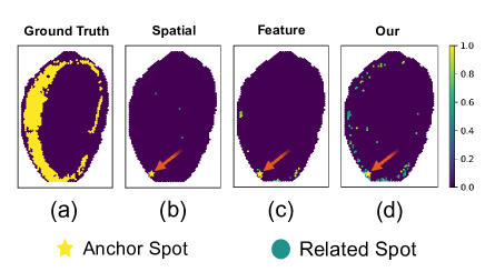
Figure 1: Visualization of adjacency graph of random anchor spots on the Human Lymph Node dataset. (a) highlights the spots with the same cell type as the anchor spots. (b) and (c) shows the related spots found by spatial and feature adjacency K-nearest neighbor (KNN) graphs, respectively. (d) shows the potential relevant spots revealed by our proposed dynamic omic-specific graph.

Technically, the current single-cell sequencing technology inevitably introduces perturbations in the sequencing data due to biological variation and other uncontrollable factors. These perturbations hide some informative semantic relations, resulting in incomplete modeling of semantic relations by the fixed KNN graph. To verify this intuition, we follow SpatialGlue (Long et al. 2024) to perform KNN to construct the RNA adjacency graph in the Human Lymph Node dataset and randomly select a sequencing spot as an anchor for visualization. As shown in Figure 1, compared with Ground Truth (GT), the spatial (Figure 1 (b)) and feature (Figure 1 (c)) adjacency graphs constructed by KNN only reveal limited connections and are limited by the spatial region obviously, e.g., the upper right area has no relevant feature points recognized in Figure 1 (c), although spots with the same type to the anchor exist there. This fixed graph structure with severe semantic information loss inevitably causes undesired performance degradation of spatial multi-omics resolved models. To address this problem, we propose an omics-specific dynamic graph architecture to denoise perturbations by learning cross-modal knowledge and thereby reveal latent semantic relations. Compared with the graph constructed by KNN, our method can learn a more informative graph structure (Figure 1 (d)) that is closer to GT.

In addition, sequencing spot annotations and the number of spot types are usually unknown in practical scenarios, which makes it difficult to provide type-related knowledge for the optimization of omics-specific graphs. Inspired by Bayesian Mixture Models (Ronen, Finder, and Freifeld 2022; Chang and Fisher III 2013; Zhao, Wen, and Han 2023), we propose a dynamic prototype contrastive learning method to address this issue. Benefiting from the adaptability of the Bayesian Gaussian Mixture Model to the number of clusters in an open Bayesian environment, the dynamic prototype contrast learning can adaptively perceive the number of cell types and optimize the learnable graph architecture to reveal potential correlations among spots.

In this paper, we propose a novel spatial multi-omics resolved framework, termed PRototype-Aware Graph Adaptive Aggregation for Spatial Multi-modal Omics Analysis (PRAGA). PRAGA learns an adaptive omics-specific graph to model spatial neighborhoods as well as latent semantic relations among spots. Moreover, a dynamic prototype contrastive learning method is proposed to optimize omics-specific graphs despite the unknown number of spot types. Extensive qualitative and quantitative experimental results demonstrate that PRAGA significantly outperforms state-of-the-art methods in aggregating spatial multi-modal omics information into spot-type-resolvable representations. Our contributions are summarised as follows:

• We propose a novel spatial multi-modal omics resolved framework PRAGA for aggregating multi-modal omics data with their corresponding spatial positions.

• We focus on latent semantic relations hidden by sequencing perturbations, which KNN fails to capture, and propose dynamic omics-specific graphs to learn these semantic relations from other omics modalities.

• We propose a learnable spatial aggregation graph structure to adaptively aggregate features and spatial information to obtain omics-specific encodings.

• We consider the common lack of biological priors in practical scenarios and propose a dynamic prototype contrastive learning to optimize PRAGA by adaptively sensing the number of sequencing point types.

Related work

Multi-omics Aggregation

Multi-modal omics aggregation aims to integrate multiple omics data from the same biological sample to analyze gene expression and regulatory processes comprehensively. Existing multi-modal omics aggregation methods can be mainly divided into three categories: 1) non-negative matrix factorization; 2) Bayesian statistics; and 3) deep learning methods. The non-negative matrix factorization decomposes multi-modal omics data into a common factor matrix to obtain a unified representation (Jin, Zhang, and Nie 2020; Zeng et al. 2019). Bayesian statistics methods fit one omics data to the conditional probability distribution of other omics but require biological priors (Kamimoto et al. 2023; Bachireddy et al. 2021). Compared with the above two methods, deep learning methods have attracted widespread attention due to their scalability and excellent performance. TotalVI (Gayoso et al. 2021) jointly models RNA and protein data into a low-dimensional space based on a variational autoencoder to obtain the comprehensive representation. MultiVI (Ashuach et al. 2023) performs independent encoders for each modality of omics data and maps the multi-modal encodings to a joint latent space. Despite integrating multi-modal omics, these methods ignore the impact of spatial location on omics features.

Spatial Resolved Omics

Recently, spatial resolved omics technologies, represented by spatial transcriptomics (Moses and Pachter 2022; Wei et al. 2022), have been proposed to associate spatial information with transcriptomic data. STAGATE (Dong and Zhang 2022) captures the local structure and spatial dependency of transcriptomic data via a graph attention network (Veličković et al. 2017). PAST (Li et al. 2023) performs a transformer architecture to capture self-similarity and global dependencies in transcriptomic data. The most advanced work SpatialGlue (Long et al. 2024) constructs a K-nearest neighbor (KNN) graph to model semantic relations and integrate spatial information with multi-modal omics through attention weights to provide a comprehensive representation. However, due to the inherent perturbations introduced during sequencing, the semantics of some omics features are disturbed and difficult to model by KNN graphs. In this paper, we propose a dynamic graph to mitigate the interference of perturbations and capture latent semantic relations through cross-modal knowledge and dynamic prototype contrastive learning.

Method

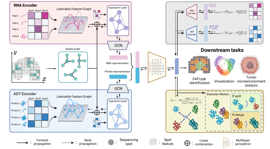
Figure 2: The framework of the proposed PRAGA. A learnable feature graph is used to explore the potential correlations between spots. The comprehensive representations of multi-modality (RNA, Protein) are obtained by aggregating modality-specific encodings, which GCNs calculate with linear combinations of learnable feature graphs and spatial adjacency graphs. The entire model is trained with a modality-specific reconstruction loss and a dynamic cluster prototype contrastive loss for the latent representation, where clusters are obtained via a Gaussian Mixture Model and optimized via split and merge operations.

Preliminaries

Spatial multi-modal omics resolve tasks aim to integrate spatial information and multi-modal omics data, such as RNA sequencing in transcriptomics, Assay for Transposase-Accessible Chromatin (ATAC) in genomics, and Antibody-Derived Tags (ADT) in proteomics, to obtain a unified latent representation. Given spatial coordinates of $N$ sequencing spots $\boldsymbol{S}=\left\{(x_{i},y_{i})\right\}_{i=1}^{N}$ and their corresponding features from $M$ modalities $\boldsymbol{F_{M}}=\left\{\boldsymbol{f_{i}^{m}}\right\}_{i=1,m=1}^{i=N,m=M}$, where $\boldsymbol{f^{m}}\in\mathbb{R}^{D_{m}}$ represent the $D_{m}$-dimensional features of the $m$ modality, usually obtained by data preprocessing such as principal component analysis (Pearson 1901) and highly variable gene screening. Spatial multi-modal omics resolve methods provide a function $\Phi$ to aggregate $\boldsymbol{F_{M}}$ and $\boldsymbol{S}$ to $D_{z}$-dimensional comprehensive latent representation $\boldsymbol{\mathcal{Z}}$:

$$\boldsymbol{\mathcal{Z}}=\Phi\left(\boldsymbol{F_{M}},\boldsymbol{S}\right).$$ (1)

The comprehensive representation $\boldsymbol{\mathcal{Z}}$ can be applied to downstream bioinformatics analysis tasks such as cell identification (Littman et al. 2021), tumor microenvironment analysis (Hunter et al. 2021; Janesick et al. 2023), etc.

PRAGA

In this paper, we propose a parameterized architecture PRAGA as the function $\Phi$ in Eq. (1) to integrate multi-modal omics data and spatial information into a comprehensive latent representation. Specifically, we first construct a dynamic omic-specific feature graph $\mathcal{G}^{F}_{m}=(\mathcal{V}^{F}_{m},\mathcal{E}^{F}_{m})$ for each modality, where $\mathcal{V}$ is the set of graph nodes and $\mathcal{E}$ is the set of undirected edges. For the convenience of formulation, we express $\mathcal{V}_{m}$ and $\mathcal{E}_{m}$ in matrix form as the omic-specific feature matrix $\boldsymbol{F_{m}}$ and adjacency matrix $\boldsymbol{A^{F}_{m}}$, i.e., $\mathcal{G}^{F}_{m}=(\boldsymbol{F_{m}},\boldsymbol{A^{F}_{m}})$. Then, we construct a K-Nearest Neighbor (KNN) spatial adjacency graph $\mathcal{G}^{S}=(\boldsymbol{S},\boldsymbol{A^{S}})$ and learn an aggregation graph $\hat{\mathcal{G}}^{F}_{m}=(\boldsymbol{F_{m}},\boldsymbol{\hat{A}^{F}_{m}})$ by combining the spatial graph $\mathcal{G}^{S}$ and the feature graph $\mathcal{G}^{F}_{m}$. Further, the GCN is performed as an encoder to encode omic features with the spatial aggregation graph $\hat{\mathcal{G}}^{F}_{m}$ for each modality. Finally, the unified comprehensive representations $\boldsymbol{\mathcal{Z}}$ are integrated from all modalities by a Multi-Layer Perceptron.

To mitigate the impact of perturbations on a single modality, we propose a reconstruction loss, $\mathcal{L}_{recon}$, using a modality-specific decoder to impart cross-modal knowledge to dynamic omic-specific graphs. Facing the challenge of unknown biological priors in practice, we propose dynamic prototype contrastive learning, which adaptively determines the number of spot types and uncovers latent semantic relationships between sequencing spots. An overview of our proposed PRAGA method is illustrated in Figure 2. The overall process of our proposed PRAGA is summarized in Algorithm 1.

Dynamic Omic-specific Graph

Limited by uncontrollable factors such as biological variation, some single-cell sequencing data are inevitably disturbed by perturbations. In this case, performing KNN to model the inter-spot semantic relations is simplicity and crudity, since it discards some informative semantic relations, especially the latent relations disturbed by sequencing perturbations. Here we provide a more fine-grained solution: building a dynamic graph structure to learn latent semantic relations while resisting sequencing perturbations by learning cross-modal knowledge.

Given a specific omics modality, such as RNA sequencing data $\boldsymbol{F_{\text{RNA}}}$ with $N$ sequencing spots, we construct a learnable parameter matrix $\boldsymbol{A^{F}_{\text{RNA}}}\in\mathbb{R}^{N\times N}$ to model the inter-spots semantic relation graph $\mathcal{G}^{F}_{\text{RNA}}=(\boldsymbol{F_{\text{RNA}}},\boldsymbol{A^{F}_{\text{RNA}}})$. The KNN undirected graph is used to initialize $\mathcal{G}^{F}_{\text{RNA}}$ to ensure initial sparsity. Specifically, for sequencing spot $i$, we set K spots with the closest Euclidean distance to its sequencing feature $\boldsymbol{f^{\text{RNA}}_{i}}$ as neighbors, where K is set to 20 following (Long et al. 2024). Then we initialize $A^{F}_{\text{RNA},i,j}$=1 if and only if sequencing spot $j$ is a neighbor of $i$, otherwise $A^{F}_{\text{RNA},i,j}$=0. The intuition behind the design of this KNN-initialized dynamic graph is to adjust the KNN graph by learning new edge weights to model the latent semantic relations disturbed by sequencing perturbations.

Spatial Aggregation Encoding

Equipped with the dynamic omic-specific graph, we construct a spatial aggregation graph to encode omics data by combining feature and spatial information. Taking RNA sequencing data $\boldsymbol{F_{\text{RNA}}}$ in transcriptomics as an example, we first initialize the learnable feature graph $\mathcal{G}^{F}_{\text{RNA}}$ and spatial adjacency graph $\mathcal{G}^{S}=(\boldsymbol{F_{\text{RNA}}},\boldsymbol{A^{S}})$ through KNN, where $\boldsymbol{A^{S}}\in\mathbb{R}^{N\times N}$ is the spatial adjacency matrix calculated based on spatial coordinates. The spatial aggregated graph $\hat{\mathcal{G}}_{\text{RNA}}=(\boldsymbol{F_{\text{RNA}}},\boldsymbol{\hat{A}_{\text{RNA}}})$ is obtained by combining $\mathcal{G}^{S}$ and $\mathcal{G}^{F}_{\text{RNA}}$ with learnable parameters:

$$\boldsymbol{\hat{A}_{\text{RNA}}}=w^{S}_{\text{RNA}}\boldsymbol{A^{S}}+w^{F}_{\text{RNA}}\boldsymbol{A^{F}_{\text{RNA}}},$$ (2)

where $w^{S}_{\text{RNA}}$ and $w^{F}_{\text{RNA}}$ are learnable parameters. Then, we perform a one-layer GCN (Kipf and Welling 2016) as an encoder to encode RNA sequencing features $\boldsymbol{F_{\text{RNA}}}$ with spatial aggregated graph $\hat{\mathcal{G}}_{\text{RNA}}$:

$$\boldsymbol{Z_{\text{RNA}}}=\text{GCN}^{en}_{\text{RNA}}(\boldsymbol{F_{\text{RNA}}},\boldsymbol{\hat{A}_{\text{RNA}}})=\boldsymbol{\hat{A}_{\text{RNA}}}\boldsymbol{F_{\text{RNA}}}\boldsymbol{W_{\text{RNA}}^{en}},$$ (3)

where $\boldsymbol{W_{\text{RNA}}^{en}}$ is a learnable parameter matrix in the encoder.

Similarly, we obtain the encoding of other omics data, e.g. $\boldsymbol{Z_{\text{ADT}}}$ and $\boldsymbol{Z_{\text{ATAC}}}$, using Eq. (2) and Eq. (3). After obtaining modality-specific encoding for all modalities $\{\boldsymbol{Z_{\text{RNA}}},\boldsymbol{Z_{\text{ADT}}},\boldsymbol{Z_{\text{ATAC}}}\}$, a Multi-Layer Perceptron (MLP) is utilized to map differential modality encoding to a unified comprehensive representation:

$$\boldsymbol{\mathcal{Z}}=\text{MLP}(\text{Concat}(\{\boldsymbol{Z_{\text{RNA}}},\boldsymbol{Z_{\text{ADT}}},\boldsymbol{Z_{\text{ATAC}}}\})),$$ (4)

where $\text{Concat}(\cdot)$ is the concatenation operation.

For each modality, we perform a modality-specific decoder, also implemented by a single-layer GCN, to reconstruct omics features from comprehensive encoding $\boldsymbol{\mathcal{Z}}$ with spatial adjacency graph $\mathcal{G}^{S}$:

$$\boldsymbol{F_{m}^{recon}}=\text{GCN}^{de}_{m}(\boldsymbol{\mathcal{Z}},\boldsymbol{A^{S}})=\boldsymbol{A^{S}}\boldsymbol{\mathcal{Z}}\boldsymbol{W_{m}^{de}},$$ (5)

where subscript $m$ present specific modality and $m\in\{\text{RNA, ADT, ATAC}\}$ in our setting. The reconstructed loss can be calculated by the mean square error between reconstructed omics features and origin omics features:

$$\mathcal{L}_{recon}=\frac{1}{M}\sum_{m=1}^{M}w_{m}\|\boldsymbol{F_{m}}-\boldsymbol{F_{m}^{recon}}\|_{2}^{2}.$$ (6)

where $w_{m}$ represents the reconstruction weight of the $m$ modality. The reconstruction loss $\mathcal{L}_{recon}$ constrains the encoding model to retain modality-specific information while providing cross-modal supervision to each omic-specific graph structure, so that the omic-specific graph can obtain knowledge from other modalities to mitigate the impact of sequencing perturbations and promote dynamic omic-specific graph to discover potential semantic relations.

Empirically, drastic changes in the adjacency graph present a risk of unstable training (Jin et al. 2020). Therefore, we calculate homogeneity loss utilizing the F-norm of the interpolated feature graph before and after the update to constrain the change of the feature graph:

$$\mathcal{L}_{h}=\frac{1}{M}\sum_{m=1}^{M}\|\boldsymbol{A^{F}_{m}}-\boldsymbol{A^{ref}_{m}}\|_{\mathcal{F}},$$ (7)

where $\boldsymbol{A^{ref}_{m}}$ is a reference graph of modal $m$, initialized in the same way as $\boldsymbol{A^{F}_{m}}$, and slowly updated by exponential moving average during the learning process of $\boldsymbol{A^{F}_{m}}$:

$$\boldsymbol{A^{ref}_{m,e}}=\begin{cases}\text{KNN }(\boldsymbol{F_{m}}),&e=1\\ \alpha\boldsymbol{A^{ref}_{m,e-1}}+(1-\alpha)\boldsymbol{A^{F}_{m,e-1}},&e>1\par\end{cases}$$ (8)

where $e$ is the training epoch index, and $\alpha$ is a hyper-parameter to control the moving speed. Homogeneity loss constrains the omics-specific graph to learn only a small number of new associated edges each time, providing interpretability for the omics-specific graph while maintaining training stability.

Dynamic Prototype Contrastive Learning

In practice, spot type annotations and even the number of spot types are often unknown, hindering the existing methods from exploring inter-spot latent relations from the spot clustering perspective. Fortunately, we draw inspiration from Bayesian Mixture Models (Ronen, Finder, and Freifeld 2022; Chang and Fisher III 2013) and propose a Bayesian Gaussian Mixture Model-based dynamic prototype contrastive learning.

For comprehensive representation $\boldsymbol{\mathcal{Z}}$ obtained by Eq. (4), we set an initial number of clusters $C$ and utilize the Gaussian Mixture Model to assign $\boldsymbol{\mathcal{Z}}$ into $C$ clusters. Note that the parameter sensitivity experiments verify the insensitivity of our method to initial $C$ values, so only a rough $C$ value is needed in practical scenarios. The mean and the number of examples in each cluster are formulated as $\boldsymbol{\mu_{c}}$ and $N_{c}$, where the subscript $c$ represents the cluster index. To dynamically adjust the number of clusters, each cluster is further divided into two sub-cluster, whose mean and the number of examples are denoted as $\boldsymbol{\mu_{c,s}}$ and $N_{c,s}$, where $s\in\{1,2\}$ is the sub-cluster index. Then, we set a split criterion for each cluster to decide whether this cluster needs to split:

$$\mathcal{S}=\frac{\Gamma(N_{c,1})L(\boldsymbol{Z_{c,1}},\nu,\kappa)\Gamma(N_{c,2})L(\boldsymbol{Z_{c,2}},\nu,\kappa)}{\Gamma(N_{c})L(\boldsymbol{Z_{c}},\nu,\kappa)},$$ (9)

where $\Gamma(\cdot)$ is the Gamma function, $L(\cdot,\nu,\kappa)$ is the marginal likelihood with a Normal Inverse Wishart (NIW) distribution as the prior, $\nu$ and $\kappa$ are hyper-parameters of NIW. If $\mathcal{S}>1$, the original cluster will be replaced by one of its sub-clusters, and the other sub-cluster is added as a new cluster:

$$\boldsymbol{\mu_{c}}:=\boldsymbol{\mu_{c,1}},\boldsymbol{\mu_{\textit{C+}1}}:=\boldsymbol{\mu_{c,2}}.$$ (10)

Similarly, a merge criterion is set to determine whether two clusters $i$ and $j$ need to be merged into one:

$$\mathcal{M}=\frac{\Gamma(N_{i}+N_{j})L(\boldsymbol{Z_{i}}\cup\boldsymbol{Z_{j}},\nu,\kappa)}{\Gamma(N_{i})L(\boldsymbol{Z_{i}},\nu,\kappa)\Gamma(N_{j})L(\boldsymbol{Z_{j}},\nu,\kappa)}.$$ (11)

The new merge cluster will replace the original two clusters with the average of the two clusters if $\mathcal{M}>1$:

$$\boldsymbol{\mu_{i}}:=\boldsymbol{\varnothing},\boldsymbol{\mu_{j}}:=\boldsymbol{\varnothing},\boldsymbol{\mu_{\textit{C}\text{-}2\text{+}1}}:=\frac{\boldsymbol{\mu_{i}}+\boldsymbol{\mu_{j}}}{2}$$ (12)

After obtaining the adjusted clusters, we assign the nearest cluster to each sequencing spot, and perform contrastive learning to further optimize learnable feature graphs with cluster centers as prototypes:

$$\mathcal{L}_{dpcl}=-\frac{1}{N}\sum_{\boldsymbol{z_{i}}\in\boldsymbol{\mathcal{Z}}}{log\frac{exp\left(\boldsymbol{z_{i}}\cdot\boldsymbol{\mu^{\ast}}/\tau\right)}{\sum_{c=1}^{c=\hat{C}}{exp\left(\boldsymbol{z_{i}}\cdot\boldsymbol{\mu_{c}}/\tau\right)}}},$$ (13)

where $\boldsymbol{\mu^{\ast}}$ is the center of the cluster closest to $\boldsymbol{z_{i}}$, $\hat{C}$ is the number of clusters updated after the spilt and merge operations, $\tau$ is the temperature hyper-parameter. Thanks to the split and merge operations, the $\mathcal{L}_{dpcl}$ can obtain an adaptive number of prototypes for contrastive learning, enabling the model to generate a resolvable comprehensive representation even if the number of categories of spots is unknown. In addition, supervision from $\mathcal{L}_{dpcl}$ also drives omic-specific graphs to learn latent semantic relations, thereby obtaining a informative omic-specific encoding.

The total loss of our method is the combination of the homogeneity loss, reconstructed loss, and contrastive learning:

$$\mathcal{L}_{Total}=\mathcal{L}_{h}+\mathcal{L}_{recon}+\beta\mathcal{L}_{dpcl},$$ (14)

where $\beta$ is the weight hyper-parameter that balances the loss component $\mathcal{L}_{dpcl}$.

Through the joint constraints of three losses $\mathcal{L}_{f}$, $\mathcal{L}_{recon}$, and $\mathcal{L}_{dpcl}$, our proposed dynamic omics-specific graph is able to resist the interference of sequencing perturbations by learning semantic knowledge from other modalities and modeling abundant semantic relations. On this basis, our proposed PRAGA framework integrates spatial information and multi-modal omics features into a unified comprehensive representation in an end-to-end manner.

Algorithm 1 PRAGA

Input: Multi-modal omics data, e.g., RNA sequencing $F_{\text{RNA}}$, Chromatin accessibility $F_{\text{ATAC}}$, Protein expression $F_{\text{ADT}}$, and their shared spatial coordinates $S$
Parameter: The total epoch $E$, a initial K, temperature coefficient $\tau$, and loss weight $\beta$.

1:  Initialize the dynamic graph $\mathcal{G}^{F}=(\boldsymbol{F},\boldsymbol{A^{F}})$ for each modality and spatial position using K-Nearest Neighbor.

2:  for $e$ in 1,2,…,$E$ do

3:     Update reference graph for each modality in Eq. (8).

4:     Calculate the $\mathcal{L}_{h}$ for each modality in Eq. (7).

5:     Construct the aggregated graph $\hat{\mathcal{G}}^{F}=(\boldsymbol{F},\boldsymbol{\hat{A}^{F}})$ for each modality in Eq. (2).

6:     Obtain modality-specific encodes $\boldsymbol{Z}_{\text{RNA}}$, $\boldsymbol{Z}_{\text{ATAC}}$, $\boldsymbol{Z}_{\text{ADT}}$ in Eq. (3).

7:     Mapping all modality-specific encodes to a unified comprehensive representation $\boldsymbol{\mathcal{Z}}$ in Eq. (4).

8:     Calculate reconstruction loss $\mathcal{L}_{recon}$ in Eq. (6).

9:     Calculate dynamic prototype contrastive learning loss $\mathcal{L}_{dpcl}$ in Eq. (13).

10:     Train PRAGA by minimizing $\mathcal{L}_{Total}$ in Eq. (14).

11:  end for

Output Unified comprehensive code $\boldsymbol{\mathcal{Z}}$

Experiments

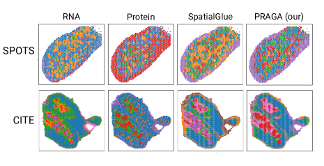
Figure 3: Visualization of qualitative experimental results on real datasets SPOTS mouse spleen (SPOTS) and mouse thymus stereo-CITE-seq (CITE).

Methods	MI(%)	NMI(%)	AMI(%)	FMI(%)	ARI(%)	V-Measure(%)	F1-Score(%)	Jaccard(%)	Compl.(%)
Human Lymph Node Dataset
MOFA+	65.06	34.91	34.49	37.67	22.73	34.91	36.96	22.67	31.88
CiteFuse	45.35	23.34	22.86	27.57	12.51	23.38	26.15	15.04	26.88
TotalVI	25.51	14.72	14.14	26.59	6.45	14.72	26.55	15.31	15.15
MultiVI	12.03	7.01	6.43	26.16	3.73	7.01	26.15	15.04	7.13
STAGATE	1.42	0.79	0.12	20.83	0.22	0.79	20.73	11.56	0.74
PAST	58.82	33.60	33.14	41.42	24.64	33.60	41.41	26.11	32.42
SpatialGlue	66.52	36.07	35.65	39.16	23.83	36.07	38.79	24.06	33.24
PRAGA	73.00	39.47	39.07	42.69	28.28	39.47	42.33	26.76	36.29
$\Delta$	+6.48	+3.40	+3.42	+1.27	+3.64	+3.40	+0.92	+0.65	+3.05
Mouse Brain Dataset
MOFA+	19.58	8.64	8.38	15.59	4.39	8.64	15.59	8.45	8.91
CiteFuse	47.48	19.46	19.05	17.96	8.24	19.46	17.89	9.82	18.63
MultiVI	17.88	8.47	8.22	18.12	3.81	8.47	17.58	9.63	9.46
STAGATE	48.45	21.25	21.03	22.36	12.21	21.25	22.36	12.59	21.76
PAST	69.49	29.13	28.76	24.54	14.63	29.13	24.54	13.99	28.50
SpatialGlue	95.54	37.83	37.53	33.78	26.33	37.83	33.01	19.77	35.14
PRAGA	95.55	39.37	39.06	35.07	27.06	39.37	35.02	21.23	37.88
$\Delta$	+0.01	+1.54	+1.53	+1.29	+0.73	+1.54	+2.01	+1.46	+2.74
Spatial Multi-modal Omics Simulation Dataset
MOFA+	1.02	0.58	-0.23	21.32	0.39	0.58	21.27	11.90	0.52
CiteFuse	1.23	0.66	-0.10	17.17	0.03	0.66	16.56	9.03	0.57
TotalVI	1.36	0.72	-0.02	15.93	-0.09	0.72	15.03	8.12	0.61
MultiVI	1.22	0.77	-0.05	25.20	-0.01	0.77	25.05	14.32	0.75
STAGATE	7.40	3.91	3.91	17.25	1.56	3.91	16.23	8.83	3.31
PAST	2.09	1.18	-0.18	19.17	0.07	1.18	18.91	10.44	1.05
SpatialGlue	150.13	96.98	96.97	98.21	97.69	96.98	98.21	96.48	96.95
PRAGA	153.35	99.06	99.05	99.47	99.32	99.06	99.47	98.95	99.08
$\Delta$	+3.22	+2.08	+2.08	+1.26	+1.63	+2.08	+1.26	+2.47	+2.13

Table 1: Quantitative experimental results with nine metrics for the human lymph node dataset, the spatial epigenome–transcriptome mouse brain dataset, and the spatial multi-omics simulation dataset. The symbol $\Delta$ indicates the performance improvement of our proposed PRAGA over the best comparison method. Underline identifies the second-best results. The best experimental results are marked in bold.

Exprimental Setups

Datasets.

We conduct quantitative and qualitative experiments on five public datasets to verify the effectiveness of the proposed method: 1) Human Lymph Node dataset (Long et al. 2024); 2) Spatial epigenome–transcriptome mouse brain dataset (Zhang et al. 2023); 3) Mouse thymus stereo-CITE-seq dataset (Liao et al. 2023); 4) SPOTS mouse spleen dataset (Ben-Chetrit et al. 2023); 5) Spatial multi-modal omics simulation datasets (Long et al. 2024). These datasets are detailed in the Appendix.

Baselines.

We compare our approach with recent advanced works, include 4 multi-modal omics methods, MOFA+ (Argelaguet et al. 2020), MultiVI (Ashuach et al. 2023), TotalVI (Gayoso et al. 2021), CiteFuse (Kim et al. 2020), 2 spatial transcriptomic methods, STAGATE (Dong and Zhang 2022), PAST (Li et al. 2023), and the latest spatial multi-omics work SpatialGlue (Long et al. 2024).

Metrics

We selected 9 different metrics to evaluate the performance of the model, including Mutual information (MI), Normalized Mutual Information (NMI), Adjusted Mutual Information (AMI), Fowlkes-Mallows Index (FMI), Adjusted Rand Index (ARI), Variation of Information Measure (V-Measure), F1-Score, Jaccard Similarity Coefficient (Jaccard), and Completeness (Compl.). Detailed experimental settings are provided in the Appendix.

Methods	MI(%)	NMI(%)	AMI(%)	FMI(%)	ARI(%)	V-Measure(%)	F1-Score(%)	Jaccard(%)	Compl.(%)
PRAGA	73.00	39.47	39.07	42.69	28.28	39.47	42.23	26.76	36.29
KNN	71.72	38.69	38.23	42.49	28.06	38.69	42.02	26.60	35.50
w/o $\mathcal{L}_{h}$	72.26	39.25	38.85	42.56	27.96	39.25	42.17	26.72	36.22
w/o $\mathcal{L}_{recon}$	64.44	35.15	34.73	38.85	23.83	35.15	38.32	23.7	32.14
w/o $\mathcal{L}_{dpcl}$	70.96	38.46	38.05	42.35	27.81	38.46	41.91	26.51	35.51

Table 2: Ablation study for our proposed learnable omics-specific graph, homogeneity loss $\mathcal{L}_{h}$, reconstruction loss $\mathcal{L}_{recon}$, and dynamic prototype contrast learning loss $\mathcal{L}_{dpcl}$ on the human lymph node dataset. KNN represents using the K-Nearest Neighbor graph to replace our proposed learnable omics feature map. w/o is the abbreviation of without. The best experimental results are marked in bold.

Qualitative experimental results

We first conducted qualitative experiments on the SPOTS mouse spleen (SPOTS) and mouse thymus stereo-CITE-seq (CITE) dataset to verify the aggregation effect of PRAGA on multi-modal omics data with spatial positions. We cluster RNA, protein, and integrated encoding obtained by the state-of-the-art method SpatialGlue and our proposed PRAGA separately, and visualize them according to spatial position in Figure 3. The visualization results show that spots of the same category integrated by PRAGA depict tighter and more continuous connections globally compared with SpatialGlue. We attribute this advantage to the learnable omic-specific graph structure and dynamic prototype contrastive learning, which enables PRAGA to resist perturbations and model latent semantic relations. More qualitative experimental results are shown in the Appendix.

Quantitative experimental results

We conduct quantitative experiments on the human lymph node dataset, the spatial epigenome–transcriptome mouse brain dataset, and the spatial multi-modal omics simulation dataset. Table 1 summarizes the quantitative experimental results of these three datasets. Note that for the spatial epigenome–transcriptome mouse brain dataset, the evaluation metrics reported in Table 1 are based on the Antibody-Derived Tag (ADT) cluster labels as Ground Truth. Benefiting from the dynamic graph structure and dynamic prototype contrastive learning, our method outperforms the baseline method on nine metrics consistently. Compared with the state-of-the-art work SpatialGlue, our proposed PRAGA achieves a significant performance improvement in F1-Score and NMI of $3.54\%$ and $3.40\%$ for the Human Lymph Node dataset, $2.01\%$ and $1.54\%$ for the Spatial epigenome–transcriptome mouse brain dataset, as well as $1.26\%$ and $2.08\%$ for the Spatial multi-modal omics simulation dataset. In addition, for several common clustering evaluation indicators such as MI, AMI, FMI, ARI, V-Measure, Jaccard similarity, and Completeness, our method is also significantly better than the baseline methods. Quantitative experimental results on the above three datasets demonstrate that our proposed PRAGA can obtain reliable comprehensive representations from spatial multi-modal omics data.

Init C	NMI	ARI	F1-Score	Jaccard	Compl.
	(%)	(%)	(%)	(%)	(%)
5	38.48	27.09	41.21	25.95	35.19
6	38.59	26.71	40.51	25.40	35.23
7	39.00	27.32	41.21	25.95	36.02
8	37.01	24.19	40.51	25.40	33.34
9	38.07	25.84	39.31	24.47	34.46
10${\dagger}$	39.47	28.28	42.23	26.76	36.29
11	38.00	26.02	39.47	24.58	34.36
12	38.84	26.79	39.49	24.40	34.89
13	39.06	27.63	41.45	26.14	35.81
14	37.95	26.62	40.20	25.16	34.52
15	38.68	27.62	42.02	26.60	35.75

Table 3: Quantitative performance of PRAGA with different initial cluster numbers. ${\dagger}$ marks the number of cluster categories in Ground Truth. The best experimental results are marked in bold.

Ablation studies

In this subsection, we verify the effectiveness of the proposed learnable feature graph, homogeneity loss, reconstruction losses, and dynamic prototype contrastive learning loss on the Human Lymph Node Dataset. As illustrated in Table 2, when the proposed learnable graph is replaced by the adjacency graph built by KNN, the performance of the PRAGA in MI, NMI, AMI, and Completeness decreases by $1.28\%$, $0.78\%$, $0.84\%$, and $0.79\%$ respectively. We explain that the cause of this performance degradation phenomenon is the loss of latent correlations between sequencing points, which are well captured and integrated with spatial information through our proposed learnable graph. The absence of homogeneity loss $\mathcal{L}_{h}$, reconstruction loss $\mathcal{L}_{recon}$, and dynamic prototype contrastive learning loss $\mathcal{L}_{dpcl}$ results in varying degrees of degradation in model performance, which in turn proves their performance contribution.

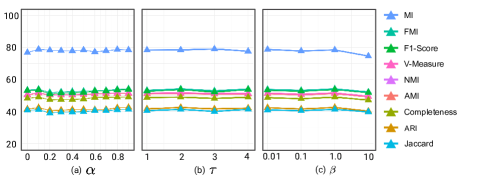
Figure 4: Effects of exponential moving average speed $\alpha$, temperature $\tau$ in $\mathcal{L}_{dpcl}$, and weight $\beta$ for $\mathcal{L}_{dpcl}$ on PRAGA performance measured by nine different metrics.

Parameter sensitivity experiments

We conduct parameter sensitivity experiments to verify the sensitivity of the performance of our proposed PRAGA to different values of hyperparameter, including the initial number of clusters $C$, exponential moving average speed $\alpha$, temperature hyperparameter $\tau$, and weight $\beta$ of $\mathcal{L}_{dpcl}$. The experiments in this subsection are conducted on the Human Lymph Node dataset.

Table 3 shows the quantitative performance of PRAGA with different initial cluster numbers. Consistent with intuition, PRAGA performs best when the number of initial clusters is the same as the number of categories in Ground Truth. Nevertheless, when the number of initial clusters differs from Ground Truth, which is also a common case in practice, PRAGA still performs well without significant performance degradation. This demonstrates that PRAGA is reliable even if the category priors of sequencing points are unknown. Figure 4 shows the effect of different values of exponential moving average speed $\alpha$, temperature $\tau$ in $\mathcal{L}_{dpcl}$, and weight $\beta$ for $\mathcal{L}_{dpcl}$ on PRAGA performance. The experimental results consistently show that PRAGA is insensitive to the values of hyperparameters.

Conclusion

In this paper, we propose a novel spatial multi-modal omics framework, named PRototype-Aware Graph Adaptative aggregation for spatial multi-modal omics analysis (PRAGA). On the one hand, PRAGA performs the dynamic feature graph to denoise the sequencing perturbations by learning cross-modal semantics. On the other hand, PRAGA integrates spatial information and multi-modal omic features to generate reliable comprehensive representations for downstream biological applications. The dynamic prototypical contrastive learning is proposed to promote the dynamic feature graph to learn abundant latent semantic relations. Qualitative and quantitative experimental results across 5 datasets demonstrate that our proposed PRAGA significantly outperforms existing State-Of-The-Art spatial multi-modal omics methods.

References

- Argelaguet et al. (2020) Argelaguet, R.; Arnol, D.; Bredikhin, D.; Deloro, Y.; Velten, B.; Marioni, J. C.; and Stegle, O. 2020. MOFA+: a statistical framework for comprehensive integration of multi-modal single-cell data. Genome biology, 21: 1–17.
- Ashuach et al. (2023) Ashuach, T.; Gabitto, M. I.; Koodli, R. V.; Saldi, G.-A.; Jordan, M. I.; and Yosef, N. 2023. MultiVI: deep generative model for the integration of multimodal data. Nature Methods, 20(8): 1222–1231.
- Bachireddy et al. (2021) Bachireddy, P.; Azizi, E.; Burdziak, C.; Nguyen, V. N.; Ennis, C. S.; Maurer, K.; Park, C. Y.; Choo, Z.-N.; Li, S.; Gohil, S. H.; et al. 2021. Mapping the evolution of T cell states during response and resistance to adoptive cellular therapy. Cell reports, 37(6).
- Ben-Chetrit et al. (2023) Ben-Chetrit, N.; Niu, X.; Swett, A. D.; Sotelo, J.; Jiao, M. S.; Stewart, C. M.; Potenski, C.; Mielinis, P.; Roelli, P.; Stoeckius, M.; et al. 2023. Integration of whole transcriptome spatial profiling with protein markers. Nature biotechnology, 41(6): 788–793.
- Chang and Fisher III (2013) Chang, J.; and Fisher III, J. W. 2013. Parallel sampling of DP mixture models using sub-cluster splits. Advances in Neural Information Processing Systems, 26.
- Dong and Zhang (2022) Dong, K.; and Zhang, S. 2022. Deciphering spatial domains from spatially resolved transcriptomics with an adaptive graph attention auto-encoder. Nature communications, 13(1): 1739.
- Gayoso et al. (2021) Gayoso, A.; Steier, Z.; Lopez, R.; Regier, J.; Nazor, K. L.; Streets, A.; and Yosef, N. 2021. Joint probabilistic modeling of single-cell multi-omic data with totalVI. Nature methods, 18(3): 272–282.
- Hunter et al. (2021) Hunter, M. V.; Moncada, R.; Weiss, J. M.; Yanai, I.; and White, R. M. 2021. Spatially resolved transcriptomics reveals the architecture of the tumor-microenvironment interface. Nature communications, 12(1): 6278.
- Janesick et al. (2023) Janesick, A.; Shelansky, R.; Gottscho, A. D.; Wagner, F.; Williams, S. R.; Rouault, M.; Beliakoff, G.; Morrison, C. A.; Oliveira, M. F.; Sicherman, J. T.; et al. 2023. High resolution mapping of the tumor microenvironment using integrated single-cell, spatial and in situ analysis. Nature Communications, 14(1): 8353.
- Jin, Zhang, and Nie (2020) Jin, S.; Zhang, L.; and Nie, Q. 2020. scAI: an unsupervised approach for the integrative analysis of parallel single-cell transcriptomic and epigenomic profiles. Genome biology, 21: 1–19.
- Jin et al. (2020) Jin, W.; Ma, Y.; Liu, X.; Tang, X.; Wang, S.; and Tang, J. 2020. Graph structure learning for robust graph neural networks. In Proceedings of the 26th ACM SIGKDD international conference on knowledge discovery & data mining, 66–74.
- Kamimoto et al. (2023) Kamimoto, K.; Stringa, B.; Hoffmann, C. M.; Jindal, K.; Solnica-Krezel, L.; and Morris, S. A. 2023. Dissecting cell identity via network inference and in silico gene perturbation. Nature, 614(7949): 742–751.
- Kim et al. (2020) Kim, H. J.; Lin, Y.; Geddes, T. A.; Yang, J. Y. H.; and Yang, P. 2020. CiteFuse enables multi-modal analysis of CITE-seq data. Bioinformatics, 36(14): 4137–4143.
- Kipf and Welling (2016) Kipf, T. N.; and Welling, M. 2016. Semi-supervised classification with graph convolutional networks. arXiv preprint arXiv:1609.02907.
- Li et al. (2023) Li, Z.; Chen, X.; Zhang, X.; Jiang, R.; and Chen, S. 2023. Latent feature extraction with a prior-based self-attention framework for spatial transcriptomics. Genome Research, 33(10): 1757–1773.
- Li et al. (2024) Li, Z.; Cui, X.; Chen, X.; Gao, Z.; Liu, Y.; Pan, Y.; Chen, S.; and Jiang, R. 2024. Cross-modality representation and multi-sample integration of spatially resolved omics data. bioRxiv, 2024–06.
- Liao et al. (2023) Liao, S.; Heng, Y.; Liu, W.; Xiang, J.; Ma, Y.; Chen, L.; Feng, X.; Jia, D.; Liang, D.; Huang, C.; et al. 2023. Integrated spatial transcriptomic and proteomic analysis of fresh frozen tissue based on stereo-seq. bioRxiv, 2023–04.
- Littman et al. (2021) Littman, R.; Hemminger, Z.; Foreman, R.; Arneson, D.; Zhang, G.; Gómez-Pinilla, F.; Yang, X.; and Wollman, R. 2021. Joint cell segmentation and cell type annotation for spatial transcriptomics. Molecular systems biology, 17(6): e10108.
- Long et al. (2024) Long, Y.; Ang, K. S.; Sethi, R.; Liao, S.; Heng, Y.; van Olst, L.; Ye, S.; Zhong, C.; Xu, H.; Zhang, D.; et al. 2024. Deciphering spatial domains from spatial multi-omics with SpatialGlue. Nature Methods, 1–10.
- Moses and Pachter (2022) Moses, L.; and Pachter, L. 2022. Museum of spatial transcriptomics. Nature methods, 19(5): 534–546.
- Pearson (1901) Pearson, K. 1901. LIII. On lines and planes of closest fit to systems of points in space. The London, Edinburgh, and Dublin philosophical magazine and journal of science, 2(11): 559–572.
- Ronen, Finder, and Freifeld (2022) Ronen, M.; Finder, S. E.; and Freifeld, O. 2022. Deepdpm: Deep clustering with an unknown number of clusters. In Proceedings of the IEEE/CVF Conference on Computer Vision and Pattern Recognition, 9861–9870.
- Veličković et al. (2017) Veličković, P.; Cucurull, G.; Casanova, A.; Romero, A.; Lio, P.; and Bengio, Y. 2017. Graph attention networks. arXiv preprint arXiv:1710.10903.
- Wei et al. (2022) Wei, X.; Fu, S.; Li, H.; Liu, Y.; Wang, S.; Feng, W.; Yang, Y.; Liu, X.; Zeng, Y.-Y.; Cheng, M.; et al. 2022. Single-cell Stereo-seq reveals induced progenitor cells involved in axolotl brain regeneration. Science, 377(6610): eabp9444.
- Xiaowei (2021) Xiaowei, A. 2021. Method of the Year 2020: Spatially resolved transcriptomics. Nat. Methods, 18(1).
- Zeng et al. (2019) Zeng, W.; Chen, X.; Duren, Z.; Wang, Y.; Jiang, R.; and Wong, W. H. 2019. DC3 is a method for deconvolution and coupled clustering from bulk and single-cell genomics data. Nature communications, 10(1): 4613.
- Zhang et al. (2023) Zhang, D.; Deng, Y.; Kukanja, P.; Agirre, E.; Bartosovic, M.; Dong, M.; Ma, C.; Ma, S.; Su, G.; Bao, S.; et al. 2023. Spatial epigenome–transcriptome co-profiling of mammalian tissues. Nature, 616(7955): 113–122.
- Zhao, Wen, and Han (2023) Zhao, B.; Wen, X.; and Han, K. 2023. Learning semi-supervised gaussian mixture models for generalized category discovery. In Proceedings of the IEEE/CVF International Conference on Computer Vision, 16623–16633.