font=small
Market Simulation under Adverse Selection
Abstract
In this paper, we study the effects of fill probabilities and adverse fills on the trading strategy simulation process. We specifically focus on a stochastic optimal control market-making problem and test the strategy on ES (E-mini S&P 500), NQ (E-mini Nasdaq 100), CL (Crude Oil) and ZN (10-Year Treasury Note), which are some of the most liquid futures contract listed on the CME (Chicago Mercantile Exchange). We provide empirical evidence which shows how fill probabilities and adverse fills can significantly effect performance, and propose a more prudent simulation framework for dealing with this. Many previous works aim to measure different types of adverse selection in the limit order book, however, they often simulate price processes and market orders independently. This has the ability to largely inflate the performance of a short-term style trading strategy. Our studies show that using more realistic fill probabilities, and tracking adverse fills, in the strategy simulation process, more accurately portrays how these types of trading strategies would perform in reality.
Keywords: Algorithmic and High-Frequency Trading, Market-Making, Adverse Selection, Stochastic Optimal Control, Market Simulation.
1 Introduction
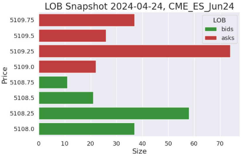
Over the last 10-15 years, algorithmic trading and high-frequency trading (HFT) has become the most common method for completing trade transactions in the worlds leading financial markets. Trading algorithms can place many different types of trade orders, but this paper will solely focus on a strategy which uses market orders (MO) and limit orders (LO) to simplify the strategy simulation process. MOs are trade orders executed at the best available prices and LOs are trade orders which rest in the limit order book (LOB) until cancelled or executed by a corresponding MO. See Figure 1 for a visual description of the LOB in the E-mini S&P 500 contract (ES), where we selected an arbitrary time during the most active US stock market trading hours (9:30 EST - 16:00 EST). We will refer to these futures contracts by their ticker symbols from now on.
Mathematical finance experts have long used stochastic processes to model the variables in algorithmic and HFT markets, where Cartea et al., (2015) brings together a whole range of Stochastic Optimal Control (SOC) examples with many variations of trading problems related to liquidation, acquisition, market making, volume-targeted trading, pairs trading, statistical arbitrage and order imbalance. The type of problem that this paper will focus on is the Market-Making (MM) style problem given in section 10.4.2 of Cartea et al., (2015), where the stochastic control is whether or not the market-maker should be posted on the best bid/ask. This problem was chosen as it highlights two of the major issues in MM that are often overlooked and oversimplified in the literature, the fill probability and the adverse fill. These can be summarized as follows:
-
•
Fill Probability: Measures the probability of a traders LO being filled when they’re posted in the LOB. This often depends on the depth in the LOB and the average trade size. As can be seen in Figure 1, one measure of the depth is the size of the bid and ask queues displayed in the LOB. One could also look at the volume traded relative to these LO sizes and in Table 1 we show the mean and median trade size per contract in four of the most liquid US futures contract, where we used LOB data from April 9th 2024 to calculate this.
Contract Mean Trade Size Median Trade Size ES 3.47 1 NQ 1.54 1 CL 1.70 1 ZN 16.01 2 Table 1: The mean and median trade sizes in four of the most liquid Chicago Mercantile Exchange (CME) futures contracts. -
•
Adverse Fills: A form of adverse selection which occurs when a passive MMs LO is picked off and they receive disadvantageous prices on their filled trade orders. In other words, immediately after their trade order is filled, their new trade position is out of the money when marked-to-market. We will show how the adverse fill occurs on the majority of trade order fills across many different assets, and based on this empirical evidence, we devised a method for including these adverse fills in our proposed trading simulation environment.
This paper will proceed as follows. We begin by discussing the significance of the paper along with a motivating example. In section 2, we will go over some of the literature on fill probabilities and adverse fills. In section 3, we introduce a SOC MM problem, which we will use for our simulation analysis. In section 4, we explain how one can create a simulation environment by discretizing the continuous processes given in section 3. Here we compare the simulation environment from Cartea et al., (2015) and Jaimungal, (2019), which we will refer to as the benchmark environment, with our improved simulation environment. Then, in section 5, we show the results of the performance of the trading strategy in both simulation environments. Lastly, we finish this paper off with some concluding remarks and ideas for future research.
1.1 Motivation and Significance of the Paper
The goal of this paper will be to contribute to the existing literature on the trading strategy simulation process by portraying a more accurate way to simulate performance. Most trading simulation frameworks in the literature model price processes and market orders independently, which can often lead to significantly inflated performance measures. The first problem here is that adverse fills often end up being excluded from the trading strategy simulation process, and, secondly, unrealistic fill probabilities are often used for every other type of trade order fill, which we will refer to as non-adverse fills. To stress the importance of tracking adverse fills in the simulation process, one must recall that in a real live trading environment, if a LO is posted at a specific price, and the price of the asset ends up going through this price, you are essentially guaranteed to have gotten a fill at a worse price than the current price. This is merely based on the rules of the LOB system. Thus, excluding any trade order fills of this nature, from the trading strategy simulation process, would create an unrealistic fill tracking process.
To go into a bit more detail on the importance of this, we give an example by analysing some limit order fill data from a professional simulator environment, using the Trading Technologies (TT) software platform. The TT Simulation environment is a SaaS technology trading platform developed by a company called Trading Technologies. As well as enabling users to trade in live markets, TT has developed its own simulation environment where users can test strategies without risking real capital. Simulation performance results here are often highly in-line with what would happen in reality, although it is important to point out that a major exception would be for strategies that aim to trade high relative volume at specific prices. Using the TT platform, we will give some empirical evidence on how often adverse and non-adverse fills occur based on a sample of simulated trades throughout a given trading day. TT can quite accurately simulate when you are likely to receive a LO fill. Put simply, whenever a LO is placed, it is placed in the LOB and given an imaginary queue position which would be the same as what one would have been given in reality. Then, a LO is considered filled when the trade order behind the imaginary order in the queue is filled in reality. This method can simulate fills quite realistically, particularly if the order size is relatively small, as this traders flow is unlikely to have effected prices in reality.
To show the likelihood of adverse fills occurring, we start by simulating a simple trading strategy in ES, NQ, CL and ZN, which posts limit orders close to the best bid/ask over a single trading day. For ES and CL, the strategy placed static orders on the bid and ask 4 ticks away from each other, in NQ 16 ticks away, and in ZN 1 tick away, while also placing orders at the same filled price again once a fill occurs at a different price. We picked these levels so that the basic posting strategy would trade low relative volume throughout the day, but at the same time, complete enough trades so that we can study the empirical limit order fill data. Each fill that precedes a disadvantageous move in the price will be considered adverse, while every other fill will be considered non-adverse. More specifically, when a LO is filled on the bid (ask) and the next new bid (ask) price is lower (higher), we consider this fill to be adverse, as the first change in the marked-to-market value of the position is negative. By marked-to-market, we used the price that the position can immediately be liquidated at using a MO, which involves crossing the spread. In order to check this, we iterated over each future LOB event until the first change in the marked-to-market value for each individual trade was nonzero. See Table 2 for the results, where we can see that a significant portion of the total number of LO fills in ES, NQ, CL and ZN were adverse.
| Trade Order Fills | ||||
|---|---|---|---|---|
| Date | Contract | Total number of LO fills | Number of adverse fills | Number of non-adverse fills |
| 2024/04/24 | ES Jun24 | 941 | 767 | 174 |
| 2024/04/25 | NQ Jun24 | 1929 | 1269 | 660 |
| 2024/04/23 | CL Jun24 | 625 | 518 | 107 |
| 2024/04/24 | ZN Jun24 | 224 | 199 | 25 |
Thus, based on the above empirical results, it is quite obvious that adverse fills could significantly effect the performance of any short-term intra-day trading strategy posting LOs, which leads us to believe that a trading simulation environment should account for this. Later on, we develop an improved simulation environment in a MM setting, where we show that the results significantly change when the simulation process tracks adverse fills, as well as utilizing non-adverse fill probabilities. We chose to perform our analysis in a MM setting, since MM strategies often trade passively, in the sense that MMs often post a large amount LO’s in the LOB and aim to trade a large amount volume throughout any given day.
2 Literature Review
There are some recent papers in optimal MM that try to incorporate the effects of fill probabilities and adverse selection into the LOB system and the trading strategy process, while there also some that use SOC theory to setup the trading problem. For example, Bulthuis et al., (2017) devises a model for analyzing LOs and MOs and how they create a permanent and temporary price impact, while also including a component for unfilled LOs, under a SOC framework. Cartea et al., 2018a developed a volume imbalance indicator to make predictions about future MOs. They designed a Markovian pure jump model of the price process, under a SOC framework, including variables such as the spread, LO and MO arrivals and volume imbalance. Roldan Contreras and Swishchuk, (2022) study various types of SOC trading problems, including MM, where they aim to portray some of the unique characteristics on how asset prices move through a dependence on recent activity and jump features. Their optimal solutions are given in terms of the arrival rates of trade orders, which they model utilizing the General Compound Hawkes Process framework. Cartea et al., 2018b , Cartea et al., (2015) and Cartea et al., (2014) develop models which assumes HFT has superior information where they can utilize this to post and cancel LOs at a quicker rate. Their models analyze factors such as arriving MOs, trade clustering and variables that can lead to a change in the shape of the LOB. They create a short-term alpha predictor with the hope of predicting future adverse fills so that they can avoid them. While collecting superior information like this may help in certain instances when making future price predictions, it cannot avoid regular random day-to-day trade order flow where it is normally too late to change the order posting strategy when random spikes in activity instantly enter the market. Predictions, in general, can often be wrong too. The instant nature of trading activity means it is often too late to change the LO posting strategy when random spikes occur. We will discuss this in more detail later from section 4 onward.
From a non SOC standpoint, there is also quite a bit of research on LOBs and fill probabilities. For a broad survey on how LOBs are modelled, see Gould et al., (2013). They discuss a large portion of the different methods used to model LOBs from a wide array of empirical and theoretical research studies. They also highlight the many shortcomings and obvious empirical facts that are yet to be included within these models. Cont and De Larrard, (2013) devised a stochastic framework for modelling the dynamics of the LOB where they made computations based on the arrival of MOs and LOs through a Markovian queueing system. Their setting made it easy to compute numerous important variables such as the distribution for the time length between changes in price, the distribution and autocorrelation for the changes in price and predictions for midprice increases/decreases. In Swishchuk and Vadori, (2017) they extend their framework by creating an arbitrary distribution for the inter-arrival times of LOB events, as well as creating a dependence structure between new and previous LOB book events, under a Markov Renewal process framework. In Swishchuk et al., (2019), they introduce two types of Hawkes processes: compound and regime-switching. Through these models they express price volatility in terms of parameters describing arrival rates and price changes. Maglaras et al., (2022) uses a recurrent neural network to predict the fill probabilities of LOs. It is the first study that directly predicts LO executions via the distribution of fill times. Arroyo et al., (2024) develops a model using survival analysis which maps time-varying features of the LOB to the distribution of fill times of limit orders. Their method uses a convolutional-transformer encoder and a monotonic neural network decoder. Lokin and Yu, (2024) proposes a queueing system method for calculating the fill probabilites of LOs posted at different levels in the LOB. Their probability model covers a wide array of scenarios including midprice changes, probabilities for orders posted at the best bid/ask and at deeper levels in the LOB. Hoffmann, (2014) devises a framework whereby you have fast and slow traders interacting together, where the fast traders can quickly revise their quotes after new information enters the market, which thus creates the ability to avoid being picked off. Cont et al., (2014) examines the impact of LOB events and that price movements occur mostly due to order flow imbalance. They portray how this could be used as a measure of adverse selection in LOs. Easley et al., (2012) discusses a method for measuring how toxic order flow can effect the MM adversely, based on volume imbalance and intensity of orders. They argue it is a good model for predicting toxic order flow over a short-term horizon. Brogaard et al., (2019) devises a model for analyzing how MOs and LOs entered by HFT and non-HFT traders induce price discovery, which they argue mostly comes from LOs, and the majority of these orders come from HFTs. They portray how a decrease in the volume of LOs entering the market often leads to increased volatility in the price.
As described above, some forms of adverse selection in relation to adverse fills have been incorporated into different frameworks in the literature. However, in terms of correcting the trading process or the LOB models for adverse fills, we have seen no prior work. No matter how good a proposed trading model is, it will be virtually impossible to avoid all adverse fills. DeLise, (2024) is the first paper to give an in-depth analysis of the likelihood of adverse fills, where they show some empirical evidence for how often adverse fills occur. They portray how the majority of trade order fills from the financial asset they study, ZN, are, in fact, adverse. We extended their ideas by also analysing the rate of adverse fills in ZN in Table 2, as well as some additional products, to further justify the empirical evidence on adverse fills, which made it clear it’s paramount to include these in any short-term trading strategy evaluation process.
3 A Stochastic Optimal Control Market-Making Problem
A MM problem, in the SOC sense, involves a financial market player who would like to maximize their terminal wealth by trading a large amount of a financial asset, often using many LOs. This type of trader is often referred to as a liquidity provider, which refers to their ability to post a large amount of LOs throughout the LOB. In the example problem we give, the control variable is whether to be posted on the best bid/ask, which is often a decision a MM tries to make. What makes this particular trading problem special is that it begins to incorporate adverse selection in the trading process, which is a big hurdle for a market-maker in reality.
Firstly, we would like to introduce the MM problem we studied, as given in Cartea et al., (2015). We begin by describing the key stochastic processes as follows,
-
•
, where , is the agents control process, which tells the market-maker whether or not to be posted at the best bid/ask.
-
•
is the agents’ controlled inventory process and is impacted by how much the agent trades.
-
•
is the controlled midprice process of the financial asset being traded, which is also impacted by how much the agent trades.
-
•
is the MO arrival process. Here, buy and sell MOs arrive at Poisson times with intensities . The MO arrival process is essentially a counting process for all the arriving MOs.
-
•
is the trade order fill process, which is also a counting process but with a dependence on the LO posting control. Here, sell and buy LOs are filled when they match with an incoming MO, .
-
•
is the agents cash process resulting from the execution strategy.
Next, we see how these processes satisfy certain SDEs as explained in Cartea et al., (2015) and Cartea et al., 2018b as follows:
-
•
The midprice process satisfies the SDE,
(1) Here, the drift is given by a long-term component and by a short-term component , which is a predictable zero-mean reverting process, and is a standard arithmetic Brownian motion.
-
•
The short-term drift component in equation (1), , can be specified in many ways and we follow the method in Cartea et al., (2015) and Cartea et al., 2018b for simplicity. Here, it’s assumed that the short-term alpha component is influenced by order flow, where it predicts the price to jump in the direction of arriving market orders. Thus, when buy MOs arrive, it creates an upward jump in the price, and when sell MOs arrive, it creates a downward jump in the price. And so, they model as a zero mean-reverting process, with jumps occurring at the arrival times of MOs, where the size of these jumps is random. Thus, in mathematical terms, satisfies the SDE,
(2) Here, and are positive constants, is a Brownian motion independent of all other processes and are i.i.d random variables also independent of all other processes representing the size of these MOs which arrive at an independent constant rate .
-
•
The controlled inventory process, which changes every time the agents posted LO is filled by an incoming MO, can be stated as follows,
(3) where () represents buy (sell) LO fills that increases (decreases) the agents inventory.
-
•
The agents cash process satisfies the SDE,
(4) Here, is the spread between the best bid and ask, and, as before, represents the counting process for filled LOs.
The agents’ performance criteria, as in Cartea et al., (2015) and Cartea et al., 2018b , is then defined as follows,
| (5) |
where , with , is a running inventory penalty which increases over time as the MMs goal is to be flat at the maturity time . The agents’ value function is next defined as
| (6) |
where is the set of admissible strategies in which and uniformly bounded from above. It is also important to note that there is an inventory constraint in this problem, whereby the inventory process has an upper and lower bound. This essentially sets the maximum position the market maker can take, long or short. Then, by applying the Dynamic Programming Principle (DPP), as explained in Cartea et al., (2015), the value function should satisfy the following Dynamic Programming Equation (DPE),
| (7) | ||||
subject to the terminal and boundary conditions:
| (8) |
Note that the expectations are over the i.i.d. random jump sizes . Each line in the DPE can be explained as follows:
-
•
Line 1: Characterizes the drift and diffusive parts of the midprice and short-term alpha processes, along alpha’s mean-reverting component. The last term on this line includes the running inventory penalty component, which only effects the inventory process.
-
•
Line 2: Characterizes the change in the value function if the agent has a sell LO posted and the effect of an arriving buy MO filling the agent’s posted sell LO. This filled LO creates a jump in the short-term alpha component. The maximisation term characterizes the agent’s control, which determines whether to post a LO at the best offer.
-
•
Line 3: Characterizes the change in the value function when an MO arrives but the agent is not posted, in which case only the short-term alpha jumps.
-
•
Line 4-5: Analogous to lines 2-3 but for the buy side of the LOB.
In Cartea et al., (2015), they use an ansatz to simplify the DPE in equation (7). This ansatz splits out the accumulated cash, the book value of the shares which are marked-to-market at the midprice and the added value from making markets optimally as follows:
| (9) |
Substituting this into the DPE in equation (7) gives us,
| (10) | ||||
subject to the terminal condition,
| (11) |
Lastly, by letting , the optimal postings can be represented in a compact form due to the structure of the maximization terms as follows,
| (12) | ||||
Here, we can see that the decision to post depends on the half-spread plus the expectation over the value functions computed at , where an arriving MO leads to a positive/negative jump in .
4 Trading Simulation Environment
In this section we discuss the trading simulation environment used to test the performance of the optimal MM strategy. In Cartea et al., (2015) and Jaimungal, (2019), they create a simulation environment in order to back-test this strategy, which we used as our benchmark. We will make one update to the benchmark by using real LOB data, rather than simulated prices. This enabled us to back-test the strategy on real financial futures contracts data later on. We will discuss the extensions we made in our improved simulation environment, which we believe more accurately portrays how this type of MM strategy would perform in reality, albeit, still with some limitations. Specifically, we will describe how our framework tracks the adverse fills, as well as an improved fill probability structure related to non-adverse fills. We will then proceed to show how this can have a major effect on the performance of the trading strategy.
First, we briefly describe the simulation environment used in Cartea et al., (2015) and Jaimungal, (2019) for the optimal MM problem described in section 3, along with the extensions we made in a little more depth. In order to simulate the performance of the MM strategy, one must first discretize the continuous-time setup given in section 3. To begin, the main components of the simulation environment are as follows,
-
•
Asset price: For this purpose, we will use Futures LOB data, which was collected at the proprietary trading firm Futures First Inc. The products we will focus on include the near-term expiry contracts for ES, NQ, CL and ZN. Market makers often tend to focus on the more liquid products like these, in particular for HFT, as it will enable them to trade more volume. We resampled our price data into a 1 second time interval, which was then subsequently used as the time step size in our discrete environment.
-
•
LO postings: Here the decision/control variable is stored, which tells us whether to be posted at the best bid/ask at any given time step. The formula for the optimal control is given in equation (12), where the values come from the numerical solution to equation (10). Since a numerical solution is discrete, the values from this solution can be used directly to determine whether to be posted or not. See Jaimungal, (2019) for how this problem is solved numerically.
-
•
Trade order fills: The benchmark trading simulation environment essentially assumes all fills are non-adverse, unless in the unlikely event a fill occurs at the exact same time as an adverse price movement. In our improved environment, however, we include adverse fills, as well as non-adverse fills, in the fill tracking process. The benchmark environment also assumes that all trade orders go to the front of the LOB queue, thus, their LOs will be the first to be filled. In most liquid financial assets, this is not very likely to occur. Based on this and using the empirical evidence from Tables 1 and 2 earlier, we will attach a binomial probability to all non-adverse fills. And so, non-adverse fills can be defined as follows,
(13) and
(14) for , where is the total number of time steps. Here, and are the counting processes for all non-adverse fills on the best ask and best bid, respectively. can be defined as:
(15) which is the probability of getting filled given the fill is non adverse. In Cartea et al., (2015) and Jaimungal, (2019), although not explicitly defined, this probability would be one, i.e., , and thus we keep it like this in the benchmark environment. Next, we will keep track of the adverse fills in the following manner:
(16) and
(17) for , where and are counting processes for adverse fills on the ask and adverse fills on the bid, respectively. Here, and represent the bid and ask prices, respectively. To understand this intuitively, at each point in time, the trading strategy has a LO posted on the best bid (ask) and the asset price at time step is lower (higher) than at time , the traders LO was then filled at the price . This is quite logical because, in reality, based on the rules of the LOB system, the asset price can not move below (above) a traders posted bid (ask) LO without filling their LO first. All other fills the trader receives will be considered non-adverse fills. Finally, in order to determine whether a fill occurred or not, we combine the two fill tracking formulas as follows,
(18) and
(19) where and are now counting processes collecting all the trade order fills that occur throughout this particular trading strategy.
For the processes involving MO arrivals, inventory, short-term alpha and cash, we follow the method given in Jaimungal, (2019), where they essentially discretize the equations (2)-(4), as well as devising a unique way to simulate MOs.
5 Results
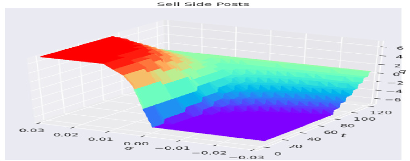
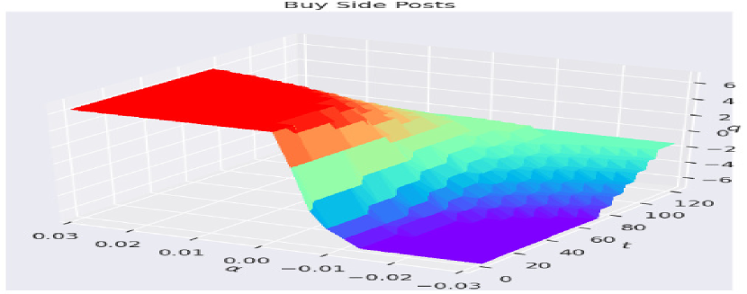
Here, we will discuss the results from testing the SOC MM strategy in our improved simulation environment and we will compare this to the benchmark environment. First, we would like to briefly summarize the numerical solution under our parameter set and we provide a visual in Figure 2, which looks similar to the solution given in Cartea et al., (2015) and Jaimungal, (2019). One can see how the optimal solution varies as a function of time (), short-term alpha () and inventory(). The left (right) Figure portrays a visual of LOs posted on the best offer (bid), where a sell (buy) LO is posted if the MMs inventory is above (below) the surface. The images look almost identical as the arrival rates of MOs are the same on both sides of the LOB. Far from maturity, the strategy is mostly independent of time, but one can see that as the MM approaches the maturity time (), the optimal strategy is essentially independent of the short-term alpha (), since the MM is solely focused on liquidating any remaining position.
As discussed earlier, the main difference in our improved simulation environment is that adverse fills are now included in the strategy simulation process, determined based on equations (16)-(17). Our aim in this section is to show how adverse fills and fill probabilities on non-adverse fills can significantly effect the performance of the trading strategy. We will discuss the results for CL in depth here, where the same repeated analysis for ES, NQ and ZN can be found in the appendix. Based on the empirical evidence for the distribution between adverse and non-adverse fills given in Table 2, we also set the non-adverse fill probability to . See Table 3, below, for a list of the parameter values used. We kept most of the parameters similar to Cartea et al., (2015) and Jaimungal, (2019), however, we decreased the time step and increased the maturity time, in order to make the length of time more realistic to the data. We also decreased the intensity of the MOs as another way to bring the distribution of adverse and non-adverse fills a bit closer to reality. A few slight adjustments to some of the other parameters were also needed to keep the numerical solution stable.
| Parameters | |||
|---|---|---|---|
| Parameter | Value | Parameter | Value |
| 0.005 | T | 120 seconds | |
| POV | 0.2 | Nq | 7 |
| 0.05 | 0.002 | ||
| 0.001 | 0.01 | ||
| 0.01 | 0 | ||
| 0.1458 | 0.1458 | ||
| Ndt | 120 | dt | 1 second |
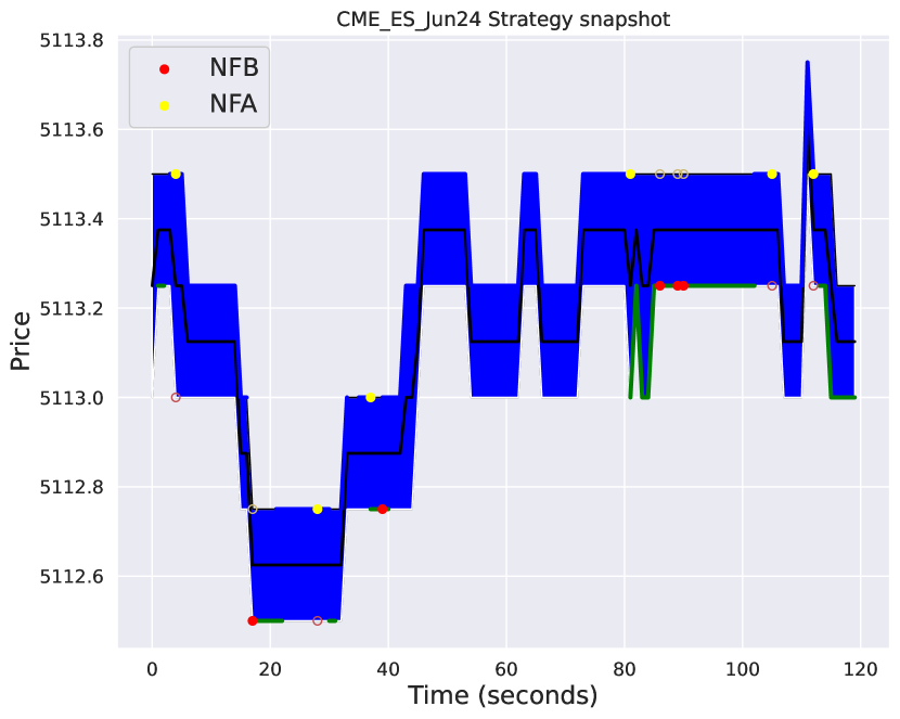
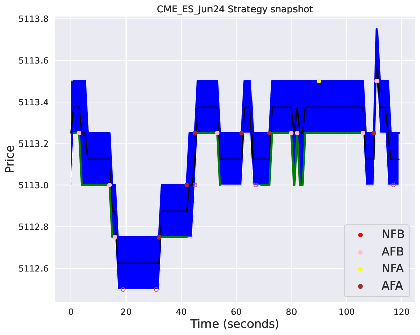
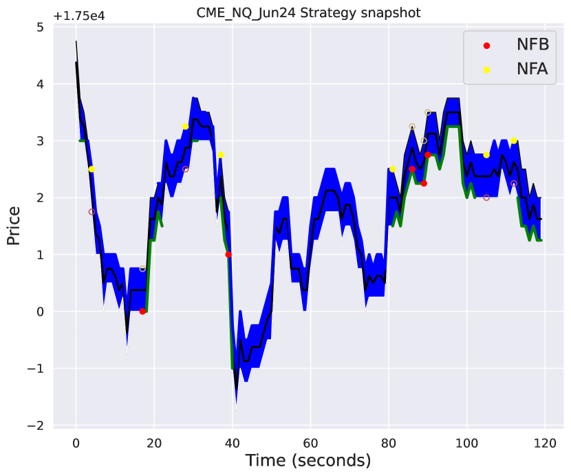
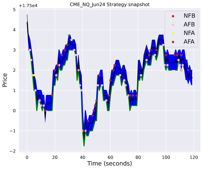
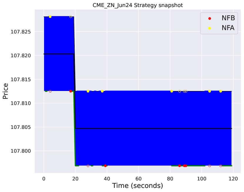
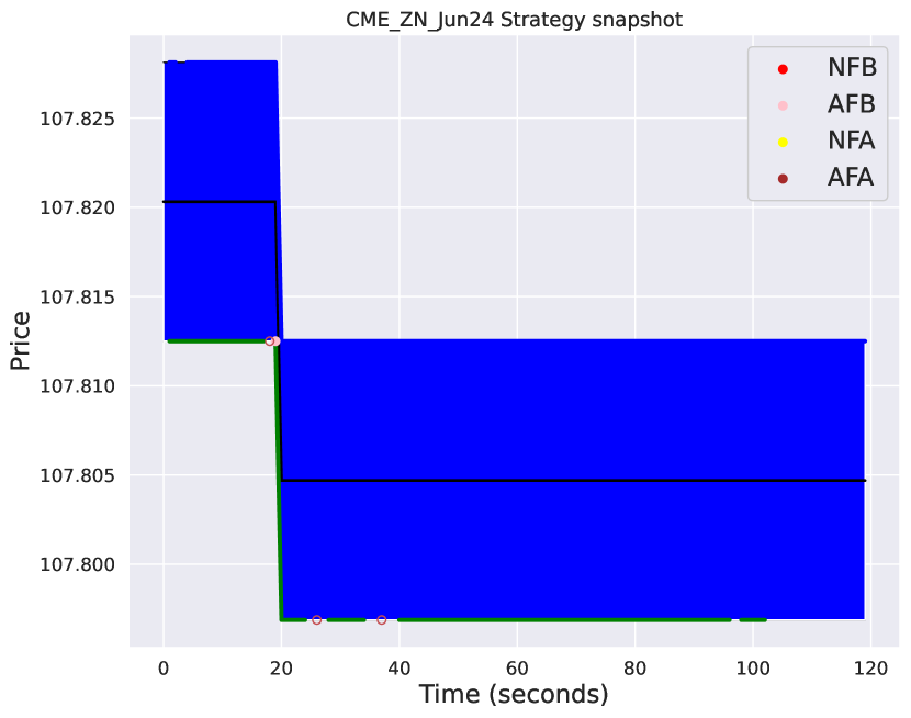
Now, we will review the strategy simulation from our improved simulation environment alongside the performance of the benchmark environment. In Figure 3, we begin by showing a snapshot of the strategy over a random 120 second path in CL, where one can see when the market-maker is posted on the best bid/ask and when they receive trade order fills. The left and right Figures show the strategy simulation in the benchmark and improved environments, respectively. Here, the green (blue) lines indicate when the market-maker is posted on the best bid (ask), the filled circles indicate when the market-makers LO is filled on the best bid/ask, and the unfilled circles indicate times the market-maker would have been filled if they had a LO posted. One noticeable feature, in the left Figure, is that whenever the agent is posted and price moves through their order, they do not automatically receive a fill. This, as we mentioned earlier, is because MOs are simulated independently from the price process in Cartea et al., (2015), Cartea et al., 2018b and Jaimungal, (2019), and is contrary to what would happen in reality. And so, all the fills in this left Figure would be referred to as non-adverse fills. In the right Figure, one can see where all the adverse fills would have occurred (denoted by AFB and AFA). Note, this can also alter the posting strategy later on because the inventory process now evolves differently to how it would in the benchmark environment.
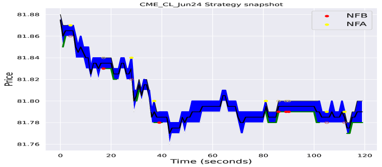
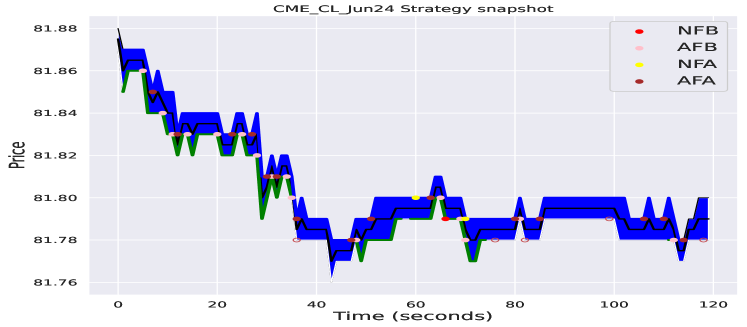
It’s quite apparent that the timing of the trade order fills has changed and many trade order fills occur at very unfavourable prices. Earlier, in our simple trading example, where we gave results in Table 2, we saw there that a overwhelming majority of the fills for the strategy simulation in CL were adverse, as well as for ES, NQ and ZN. This test was also conducted on the exact same trading day as this simulation. In Table 4, we show the number of each type of fill that occurred within our improved simulation environment. We can see that using a much lower non-adverse fill probability of created a similar distribution of fills between non-adverse fills and adverse fills as in Table 2, and we will soon see that the overall performance has now dropped significantly. This trend also persists in the strategy simulations using ES, NQ and ZN data, as can be seen in the appendix. Based on our empirical evidence, we believe these results more accurately portray how the strategy would perform in reality. However, we may not want to be overly pessimistic by thinking the SOC MM strategy should have the same number of adverse fills as the basic posting strategy, because the SOC MM model has a short-term alpha predictor which could potentially predict some of these adverse fills. However, it’s extremely unlikely that any short-term alpha predictor could foresee all future adverse fills.
| Fill Type | Amount |
|---|---|
| AFA | 3950 |
| NFA | 825 |
| AFB | 3943 |
| NFB | 813 |
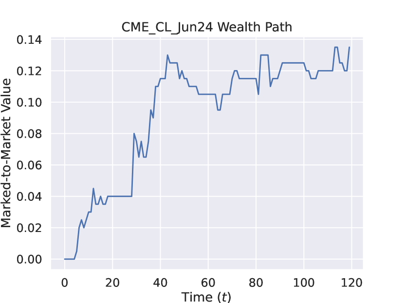
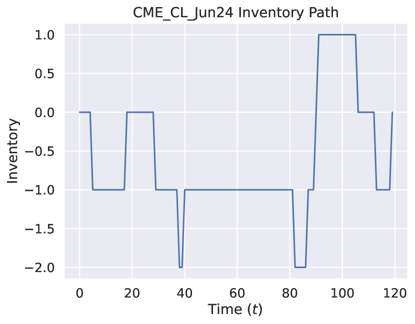
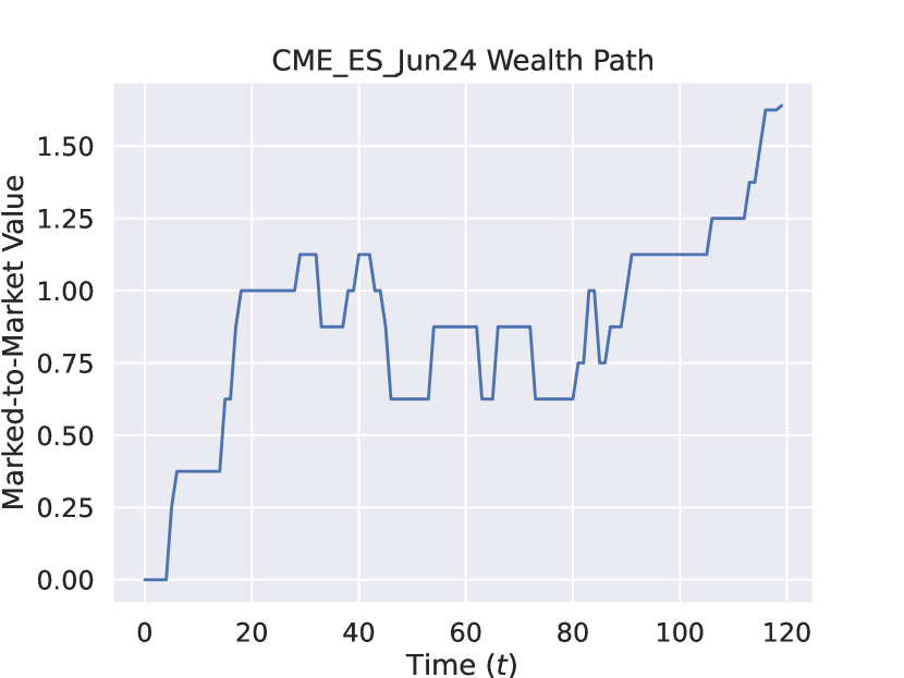
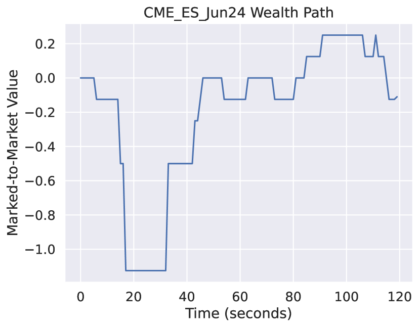
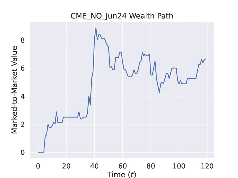
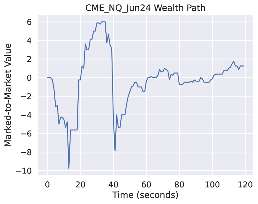
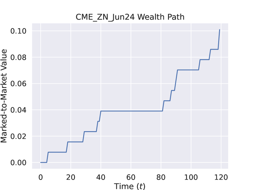
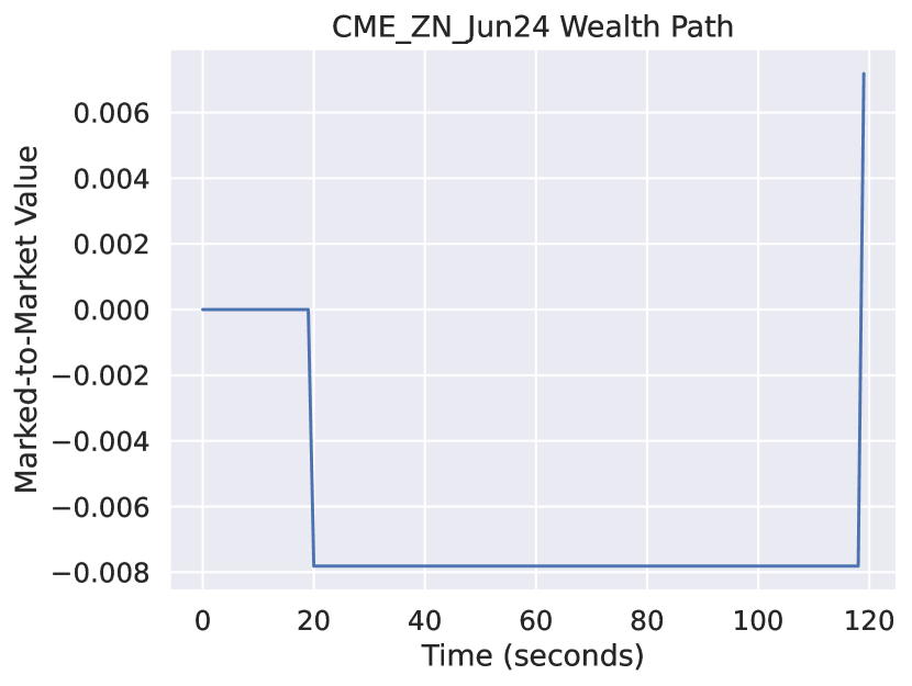
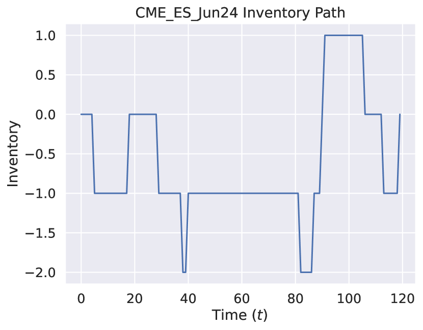
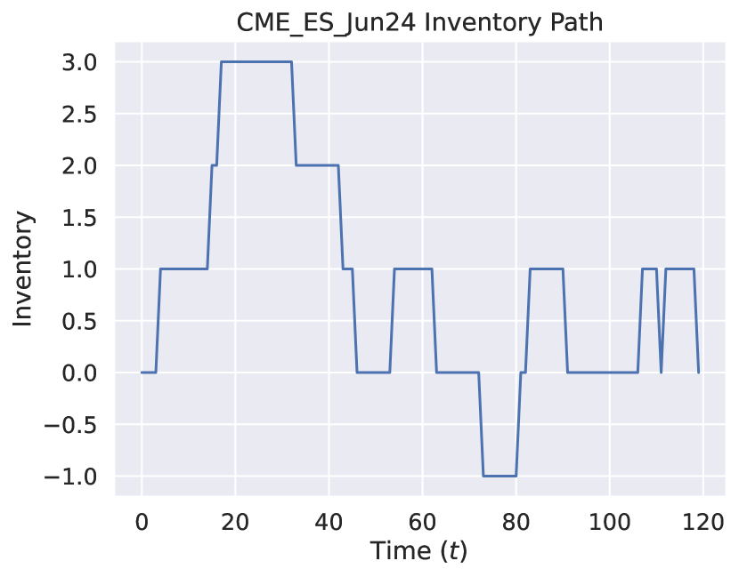
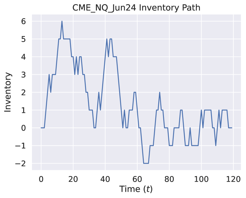
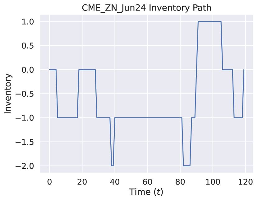
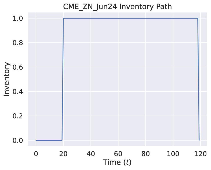
Next, in Figure 4, one can see the wealth and inventory path for the same random 120 second run of the strategy. Here, again, the left and right figures are under the benchmark and improved simulation environments, respectively. The wealth path is marked-to-market at each time step as in equation (4) and the inventory path changes whenever a trade order fill is received as in equation (3). Here, the market-makers wealth path in the left Figure finishes positive, and in the right Figure it finishes negative, over the same 120 second path. The inventory paths’ show that the benchmark environment traded a lot less than our improved environment, which is mostly due to the additional adverse fills this trader received. The additional adverse fills also significantly outweighed the reduced number of non-adverse fills. And so, it’s quite apparent that these paths now evolve very differently. Lower non-adverse fill probabilities and adverse fills has significantly effected how these processes evolved.
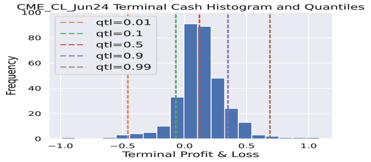
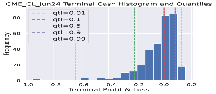
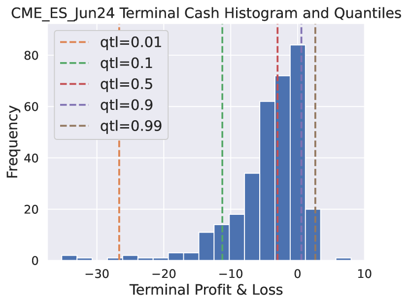
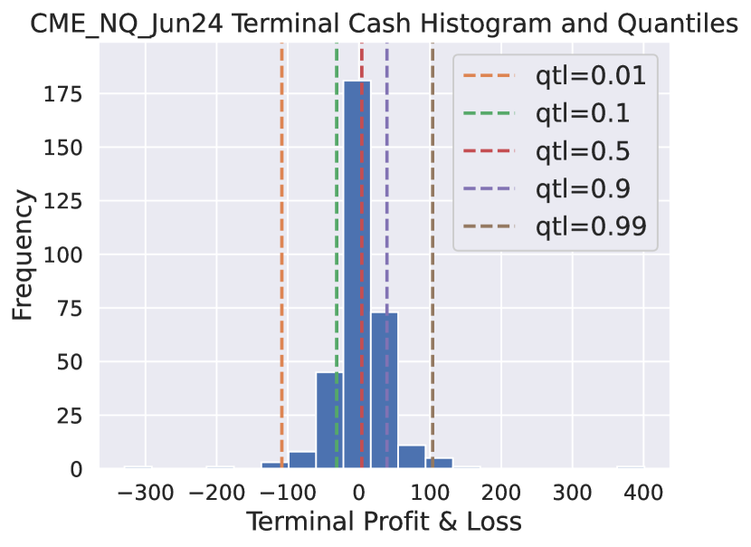
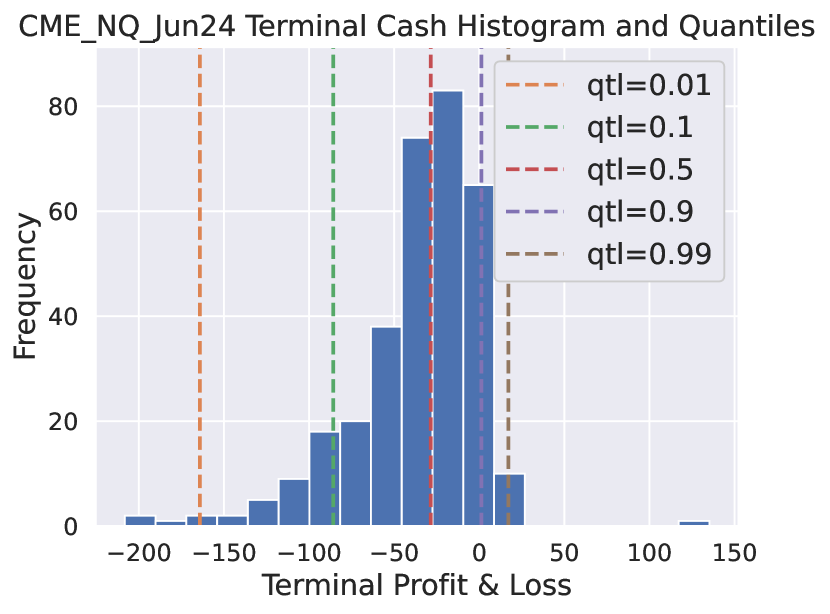
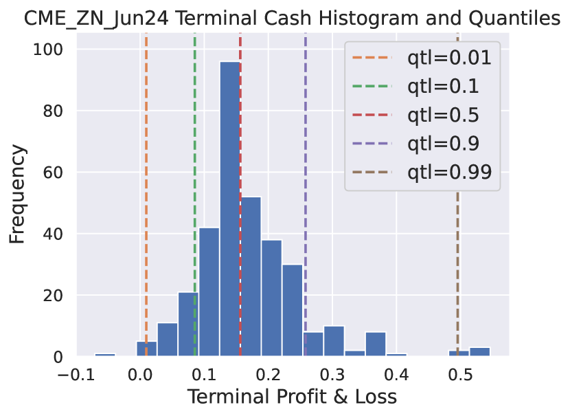
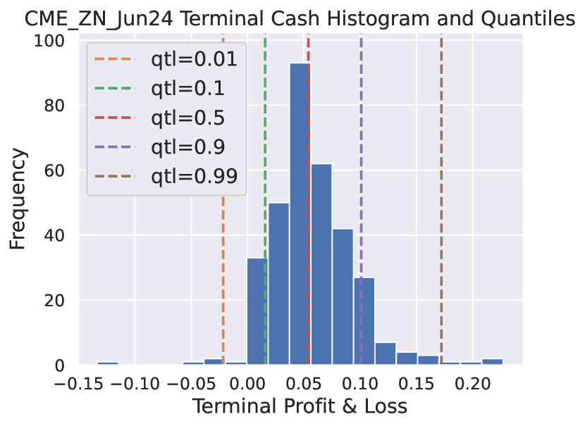
In order to tell the full story, we show a histogram, in Figure 5, of the terminal cash values from all 330 simulation runs of the strategy over this trading day. Each bin indicates how often the strategy paths attained a certain P&L. Here, again, the left and right Figures show the benchmark and improved simulation environments, respectively. One can see that, overall, the strategy performed reasonably well in the benchmark environment and much worse in our improved environment. We believe the performance metric in the benchmark environment is over-inflated, as the market-maker received a lot more non-adverse fills than likely in reality, as well not receiving any adverse fills, which clearly significantly effects the performance. In the right Figure, we can see that the strategy does not perform as well and regularly suffers large losses, relatively speaking. This confirms to us that simulating the performance of a short-term style trading strategy, in particular one involving posting many LOs, is very misleading if it does not track adverse fills and include more accurate non-adverse fill probabilities. This is just as evident in ES, NQ and ZN, where similar results for these assets can be seen in the appendix.


6 Conclusion and Future Recommendations
In this paper we simulated the performance of a SOC optimal MM strategy that both included and excluded adverse fills, as well as adjusting the probability of a non-adverse fill. Many MM style strategies often trade passively by posting many LOs throughout the LOB, thus the results here are particularly relevant to these types of strategies, but also to any trading strategy that posts a large amount LOs. Models in mathematical finance often make simplifying assumptions in order to find robust solutions to a problem and while many don’t often effect the overall performance too much, some certainly can. In our setting, modelling the price process and the arrival of MOs independently can create large inaccuracies, which is clear from our simulation results. Specifically, our finding shows that excluding adverse fills and non-adverse fill probabilities can significantly inflate the performance of a trading strategy. Adverse trade order fills are never completely avoidable for a trader who devises a LO posting strategy and are particularly apparent in short-term strategies. Although we can try to predict short-term price movements using methods like the short-term alpha predictor given in Cartea et al., (2015) and Cartea et al., 2018b , large orders often randomly enter the market taking out price levels on a whim. Thus, if a MM or trader is posted at these price levels they will receive adverse fills as there usually isn’t enough time to cancel the orders, regardless of some of the speed advantageous some HFTs may have.
In regard to future research recommendations, we think the results could be improved if a more dynamic MM model were used, where the MM can update the important parameters over time. It is clear from our analysis and the literature that LOB data has a clustering effect, thus this could enable the MM to update their non-adverse fill probabilities, as well as improving the short-term alpha predictors ability to predict adverse moves. Papers like Arroyo et al., (2024) and Maglaras et al., (2022) are some new initial works that aim to estimate fill probabilities using deep learning approaches, which seem to develop some promising ideas for devising a more dynamic model. One should also assess the performance of any short-term alpha predictor used to predict adverse moves, as this is one of the key components of the model in this paper. In the SOC framework, this simple short-term alpha predictor helped bring tractable results, but it is unlikely to be that simple to make such price predictions in reality. Lastly, one could also try to improve the price process modelling aspect, by using a jump-diffusion or Levy-style model. These price processes have been proven to more accurately mimic LOB dynamics rather than the general diffusion models, although sometimes more difficult to apply directly in a SOC model.
Acknowledgements
We would like to thank MITACS and NSERC for research funding. We would specifically like to thank Futures First for collaborating in this MITACS project, where we would also like to give a special mention to Timothy DeLise (PhD candidate at the University of Montreal and former MITACS participant in projects at Futures First) and Myles Sjogren (Quantitative Analyst at Futures First) in helping to set-up parts of the coding framework for deploying the basic posting algorithm described in section 1.1.
Declarations of Interest
The authors declare no conflicts of interest.
References
- Arroyo et al., (2024) Arroyo, A., Cartea, A., Moreno-Pino, F., and Zohren, S. (2024). Deep attentive survival analysis in limit order books: Estimating fill probabilities with convolutional-transformers. Quantitative Finance, 24(1):35–57.
- Brogaard et al., (2019) Brogaard, J., Hendershott, T., and Riordan, R. (2019). Price discovery without trading: Evidence from limit orders. The Journal of Finance, 74(4):1621–1658.
- Bulthuis et al., (2017) Bulthuis, B., Concha, J., Leung, T., and Ward, B. (2017). Optimal execution of limit and market orders with trade director, speed limiter, and fill uncertainty. International Journal of Financial Engineering, 4(02n03):1750020.
- (4) Cartea, A., Donnelly, R., and Jaimungal, S. (2018a). Enhancing trading strategies with order book signals. Applied Mathematical Finance, 25(1):1–35.
- Cartea et al., (2015) Cartea, Á., Jaimungal, S., and Penalva, J. (2015). Algorithmic and high-frequency trading. Cambridge University Press.
- Cartea et al., (2014) Cartea, Á., Jaimungal, S., and Ricci, J. (2014). Buy low, sell high: A high frequency trading perspective. SIAM Journal on Financial Mathematics, 5(1):415–444.
- (7) Cartea, A., Jaimungal, S., and Ricci, J. (2018b). Algorithmic trading, stochastic control, and mutually exciting processes. SIAM review, 60(3):673–703.
- Cont and De Larrard, (2013) Cont, R. and De Larrard, A. (2013). Price dynamics in a markovian limit order market. SIAM Journal on Financial Mathematics, 4(1):1–25.
- Cont et al., (2014) Cont, R., Kukanov, A., and Stoikov, S. (2014). The price impact of order book events. Journal of financial econometrics, 12(1):47–88.
- DeLise, (2024) DeLise, T. (2024). The negative drift of a limit order fill. arXiv preprint arXiv:2407.16527.
- Easley et al., (2012) Easley, D., López de Prado, M. M., and O’Hara, M. (2012). Flow toxicity and liquidity in a high-frequency world. The Review of Financial Studies, 25(5):1457–1493.
- Gould et al., (2013) Gould, M. D., Porter, M. A., Williams, S., McDonald, M., Fenn, D. J., and Howison, S. D. (2013). Limit order books. Quantitative Finance, 13(11):1709–1742.
- Hoffmann, (2014) Hoffmann, P. (2014). A dynamic limit order market with fast and slow traders. Journal of Financial Economics, 113(1):156–169.
- Jaimungal, (2019) Jaimungal, S. (2019). Market making at the touch with short-term alpha (chap 10.4.2). https://gist.github.com/sebjai.
- Lokin and Yu, (2024) Lokin, F. and Yu, F. (2024). Fill probabilities in a limit order book with state-dependent stochastic order flows. arXiv preprint arXiv:2403.02572.
- Maglaras et al., (2022) Maglaras, C., Moallemi, C. C., and Wang, M. (2022). A deep learning approach to estimating fill probabilities in a limit order book. Quantitative Finance, 22(11):1989–2003.
- Roldan Contreras and Swishchuk, (2022) Roldan Contreras, A. and Swishchuk, A. (2022). Optimal liquidation, acquisition and market making problems in HFT under Hawkes models for LOB. Risks, 10(8):160.
- Swishchuk et al., (2019) Swishchuk, A., Remillard, B., Elliott, R., and Chavez-Casillas, J. (2019). Compound Hawkes processes in limit order books. In Financial Mathematics, Volatility and Covariance Modelling, pages 191–214. Routledge.
- Swishchuk and Vadori, (2017) Swishchuk, A. and Vadori, N. (2017). A semi-Markovian modeling of limit order markets. SIAM Journal on Financial Mathematics, 8(1):240–273.
Appendix A Appendix: ES, NQ and ZN Strategy Simulations


| Fill Type | Amount | Fill Type | Amount | Fill Type | Amount |
|---|---|---|---|---|---|
| AFA | 5904 | AFA | 12319 | AFA | 478 |
| NFA | 789 | NFA | 840 | NFA | 825 |
| AFB | 5873 | AFB | 12370 | AFB | 468 |
| NFB | 774 | NFB | 781 | NFB | 821 |